a finite-volume, incompressible navier stokes model for...

JOURNAL OF GEOPHYSICAL RESEARCH, VOL. 102, NO. C3, PAGES 5753-5766, MARCH 15, 1997

A finite-volume, incompressible Navier Stokes model for studies of the ocean on parallel computers

John Marshall, Alistair Adcroft, Chris Hill, Lev Perelman, and Curt Heisey Department of Earth, Atmospheric and Planetary Sciences, Massachusetts Institute of Technology, Cambridge

Abstract. The numerical implementation of an ocean model based on the incompressible Navier Stokes equations which is designed for studies of the ocean circulation on horizontal scales less than the depth of the ocean right up to global scale is described. A "pressure correction" method is used which is solved as a Poisson equation for the pressure field with Neumann boundary conditions in a geometry as complicated as that of the ocean basins. A major objective of the study is to make this inversion, and hence nonhydrostatic ocean modeling, efficient on parallel computers. The pressure field is separated into surface, hydrostatic, and nonhydrostatic components. First, as in hydrostatic models, a two-dimensional problem is inverted for the surface pressure which is then made use of in the three-dimensional inversion for the nonhydrostatic pressure. Preconditioned conjugate-gradient iteration is used to invert symmetric elliptic operators in both two and three dimensions. Physically motivated preconditioners are designed which are efficient at reducing computation and minimizing communication between processors. Our method exploits the fact that as the horizontal scale of the motion becomes very much larger than the vertical scale, the motion becomes more and more hydrostatic and the three- dimensional Poisson operator becomes increasingly anisotropic and dominated by the vertical axis. Accordingly, a preconditioner is used which, in the hydrostatic limit, is an exact integral of the Poisson operator and so leads to a single algorithm that seamlessly moves from nonhydrostatic to hydrostatic limits. Thus in the hydrostatic limit the model is "fast," competitive with the fastest ocean climate models in use today based on the hydrostatic primitive equations. But as the resolution is increased, the model dynamics asymptote smoothly to the Navier Stokes equations and so can be used to address small- scale processes. A "finite-volume" approach is employed to discretize the model in space in which property fluxes are defined normal to faces that delineate the volumes. The method makes possible a novel treatment of the boundary in which cells abutting the bottom or coast may take on irregular shapes and be "shaved" to fit the boundary. The algorithm can conveniently exploit massively parallel computers and suggests a domain decomposition which allocates vertical columns of ocean to each processing unit. The resulting model, which can handle arbitrarily complex geometry, is efficient and scalable and has been mapped on to massively parallel multiprocessors such as the Connection Machine (CM5) using data-parallel FORTRAN and the Massachusetts Institute of Technology data-flow machine MONSOON using the implicitly parallel language Id.

1. Introduction

Details of the numerical implementation of a model which has been designed for the study of dynamical processes in the ocean from the convective, through the geostrophic eddy, up to global scale are set out. The "kernel" algorithm solves the incompressible Navier Stokes equations on the sphere, in a geometry as complicated as that of the ocean basins with irregular coastlines and islands. (Here we use the term "Navier Stokes" to signify that the full nonhydrostatic equations are being employed; it does not imply a particular constitutive relation. The relevant equations for modeling the full complexity of the ocean include, as here, active tracers such as temperature and salt.) It builds on ideas developed in the computational fluid community. The numerical challenge is to ensure that the evolving velocity field remains nondivergent. Most

Copyright 1997 by the American Geophysical Union.

Paper number 96JC02775. 0148-0227/97/96JC-02775509.00

procedures, including the one employed here, are variants on a theme set out by Harlow and Welch [1965] and Williams [1969], in which a "pressure correction" to the velocity field is used to guarantee nondivergence; a useful review of these methods is given by Dukowicz and Dvinsky [1992]. The correction step is equivalent to, and is solved as, a Poisson equation for the pressure field with Neumann boundary conditions. This Poisson inversion is the most computationally demanding part of the algorithm and, because it is not localized in space, presents the biggest challenge in mapping it onto parallel computers since it demands "communication" across the grid to the boundary and hence between processors. We set out here a method for solving this Poisson equation which exploits knowledge of the dynamics (by separating the pressure field into hydrostatic, nonhydrostatic, and surface pressure components) and the geometry of the ocean basins (they are much wider than they are deep) and naturally lends itself to data- parallel implementation.

The account that follows is self-contained but is closely re-

5753

5754 MARSHALL ET AL.: FINITE-VOLUME OCEAN MODEL

lated to a companion paper, Marshall et al. [this issue], in which the assumptions inherent in the hydrostatic primitive equations (HPEs) are reviewed and consistent hydrostatic (HPE), quasi- hydrostatic (QH), and Navier Stokes (NH) equation sets are set out. The kernel algorithm described is firmly rooted in the incompressible Navier Stokes equations but can be used to step forward HPE and QH as well as NH. Along the way we will arrive at a deeper understanding of the connection between the Navier Stokes equations and more approximate forms, both with respect to the dynamics they represent and the algorithms employed to solve them.

Any practical numerical rendition involves a series of com- promises. Our guiding principle has been to devise methods which, as far as is possible, are competitive across a large range of scales from L -< H, the depth of the ocean, right up to horizontal resolutions L >_ L,, coarser than the radius of deformation. We did not want to make the hydrostatic assump- tion a priori, since it precludes the study of many interesting small-scale phenomena. Rather, it was important to us that our approach be also well-suited to the convective, nonhydrostatic limit. We therefore adopt height as a vertical coordinate and employ a "finite-volume" approach, in which property fluxes are defined normal to the faces that define the volumes, leading to a very natural and robust discrete analogue of "divergence." In the special case that the volumes are of regular shape, the arrangement of the model variables in the horizontal reduces to a "C" grid, using the nomenclature of Arakawa and Lamb [1976], and so carries with it well-documented strengths and weaknesses in the treatment of gravity, inertial, and Rossby wave modes. But the finite-volume method makes possible a novel treatment of the boundary in which volumes abutting the bottom or coast may take on irregular shapes and so be "shaved" to fit the boundary; this aspect of the model is discussed in detail elsewhere by Adcroft et al. [1996]. The model is thus particularly adept at the representation of complex geometry typical of ocean basins and endows it with some of the advantages of terrain-following coordinates without any of their disadvantages.

The variables are stepped forward in time using a quasi- second-order Adams-Bashforth time-stepping scheme. The pressure field, which ensures that evolving currents remain nondivergent, is found by inversion of elliptic operators. In HPE and QH a two-dimensional (2-D) elliptic problem must be inverted; in NH the elliptic problem is three-dimensional (3-D). A major objective of our study has been to make this 3-D inversion, the "overhead" of NH, efficient and hence to make nonhydrostatic modeling affordable. The pressure field is separated into surface pressure Ps, hydrostatic pressure PHi-, and nonhydrostatic pressure P NH and the component parts are found sequentially. In the 3-D inversion for P N• a preconditioner is used which, in the hydrostatic limit, is an exact integral of the elliptic operator and so leads to an algorithm that seamlessly moves from nonhydrostatic to hydrostatic limits. Thus, in the hydrostatic limit, NH is "fast," competitive with the fastest ocean climate models in use today based on the HPEs. But as the resolution is increased, the model dynamics asymptotes smoothly to the Navier Stokes equations. Finally, the inversion methods developed here may be of wider interest because elliptic equations of the same form arise in other applications, for example, in "electrostatics" (the calculation of emf in the ocean induced by ocean currents moving in the Earth's mag- netic field, as measured in submerged cables on the seafloor;

see Flosadottir et al. [1996]) and "potential vorticity inversions" for balanced flow.

The paper is set out as follows. In section 2 we briefly review the incompressible Navier Stokes equations that are at the heart of our model. In section 3 we outline a numerical strategy for solving NH, HPE, and QH and the finite-volume methods used to discretize our problem in space. In section 4 the preconditioned conjugate-gradient methods used to invert 2-D and 3-D elliptic equations are described, and in section 5 we discuss the mapping of the algorithm onto a massively parallel machine, the Connection Machine (CM5) programmed in data-parallel FORTRAN.

2. Incompressible Navier Stokes Model 2.1. Equations

The state of the ocean at any time is characterized by the three-dimensional distribution of currents v, potential temperature T, salinity S, pressure p, and density p. The equations that govern the evolution of these fields, obtained by applying the laws of classical mechanics and thermodynamics to an incompressible Boussinesq fluid, are, using height as the vertical coordinate,

Motion

Continuity

Heat

Salt

Equation of state

where

OVh = Gv h - Vhp ot

ow op --• Sw Ot Oz

V.v=0 (2)

OT (3) ot

os

o•-= Gs (4)

p = p(T, S, p) (5)

V : (Vh, 142) = (/.•, U, 142) (6)

is the velocity in the horizontal (indicated by the subscript h) and vertical direction z, respectively, the pressure is

Pref

where •p is the deviation of the pressure from that of a resting stratified ocean and Pref is a constant reference density, and

= (Gu, Gw) (7)

represent inertial, Coriolis, metric, gravitational, and forcing/ dissipation terms in the zonal, meridional, and vertical directions. To avoid duplication, we do not explicitly write out the G here but refer the reader to (14)-(18) of Marshall et al. [this

MARSHALL ET AL.' FINITE-VOLUME OCEAN MODEL 5755

issue]. There the incompressible Navier Stokes equations .... '••._.............••rigidlid (NH) are set out and discussed in detail along with the more approximate forms, HPE and QH.

Equations (1)-(4) are prognostic in (u, v, w), T, and S and diagnostic in p andp. The density is obtained from an equation of state (5). An equation for pressure is obtained by taking the divergence of (1) and invoking continuity (2) leading to the Poisson equation:

= v. (8)

The homogeneous Neumann boundary conditions that go z

along with (8) and strategies for solving (8) are discussed in • some length by Marshall et al. [this issue]. q• Our objective here is to numerically solve discrete forms of

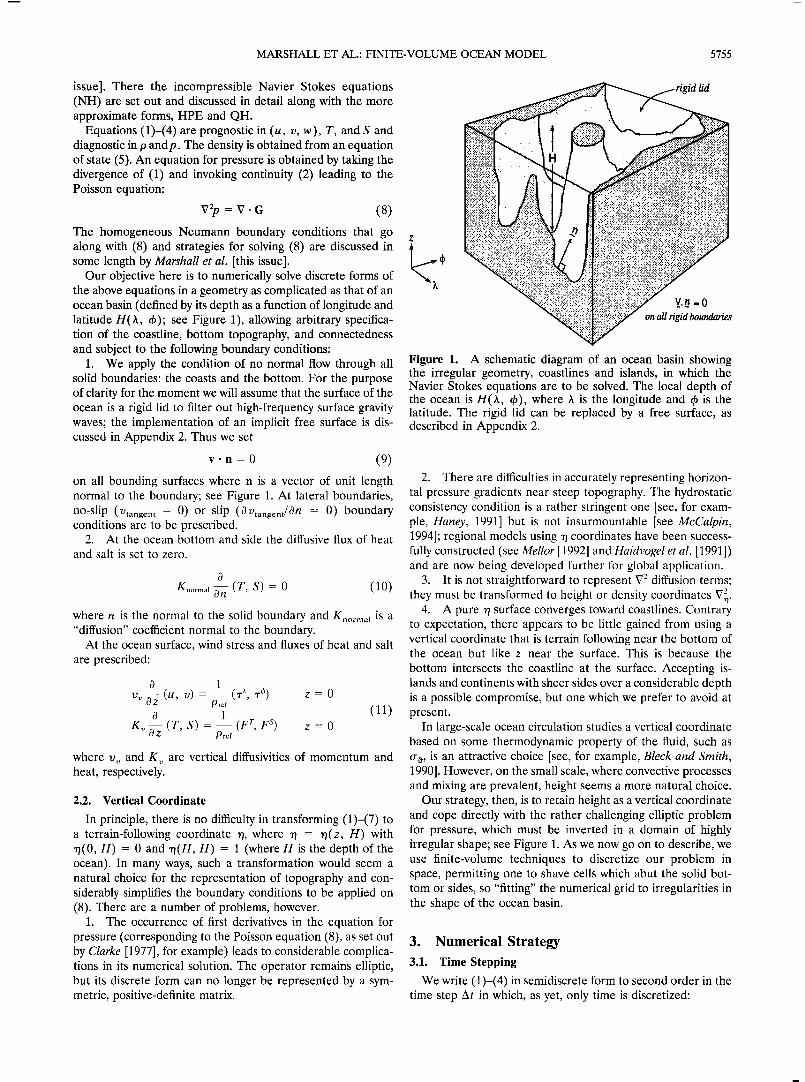
the above equations in a geometry as complicated as that of an ocean basin (defined by its depth as a function of longitude and latitude H()t, &); see Figure 1), allowing arbitrary specifica- on all rigid boundaries tion of the coastline, bottom topography, and connectedness and subject to the following boundary conditions:

1. We apply the condition of no normal flow through all solid boundaries: the coasts and the bottom. For the purpose of clarity for the moment we will assume that the surface of the ocean is a rigid lid to filter out high-frequency surface gravity waves; the implementation of an implicit free surface is discussed in Appendix 2. Thus we set

v-n-0 (9)

on all bounding surfaces where n is a vector of unit length normal to the boundary; see Figure 1. At lateral boundaries, no-slip (Utangen t = 0) or slip (0Vtangent/0n = 0) boundary conditions are to be prescribed.

2. At the ocean bottom and side the diffusive flux of heat

and salt is set to zero.

0

g ....... 1 •-(r, S): 0 (10)

where n is the normal to the solid boundary and K ..... •is a "diffusion" coefficient normal to the boundary.

At the ocean surface, wind stress and fluxes of heat and salt are prescribed:

0 1 = ( r •, r •) z = 0

0 1 (11) = -- (F r, F s) z: 0 K•, •ZZ (r , S) Pref

where u, and K,, are vertical diffusivities of momentum and heat, respectively.

2.2. Vertical Coordinate

In principle, there is no difficulty in transforming (1)-(7) to a terrain-following coordinate r/, where r/ = r/(z, H) with r/(0, H) = 0 and r/(H, H) = 1 (where H is the depth of the ocean). In many ways, such a transformation would seem a natural choice for the representation of topography and con- siderably simplifies the boundary conditions to be applied on (8). There are a number of problems, however.

1. The occurrence of first derivatives in the equation for pressure (corresponding to the Poisson equation (8), as set out by Clarke [1977], for example) leads to considerable complica- tions in its numerical solution. The operator remains elliptic, but its discrete form can no longer be represented by a symmetric, positive-definite matrix.

Figure 1. A schematic diagram of an ocean basin showing the irregular geometry, coastlines and islands, in which the Navier Stokes equations are to be solved. The local depth of the ocean is H()t, •), where )t is the longitude and • is the latitude. The rigid lid can be replaced by a free surface, as described in Appendix 2.

2. There are difficulties in accurately representing horizontal pressure gradients near steep topography. The hydrostatic consistency condition is a rather stringent one [see, for example, Haney, 1991] but is not insurmountable [see McCalpin, 1994]' regional models using r/coordinates have been success- fully constructed (see Mellor [1992] and Haidvogel et al. [ 1991]) and are now being developed further for global application.

3. It is not straightforward to represent V 2 diffusion terms; they must be transformed to height or density coordinates

4. A pure r/surface converges toward coastlines. Contrary to expectation, there appears to be little gained from using a vertical coordinate that is terrain following near the bottom of the ocean but like z near the surface. This is because the

bottom intersects the coastline at the surface. Accepting islands and continents with sheer sides over a considerable depth is a possible compromise, but one which we prefer to avoid at present.

In large-scale ocean circulation studies a vertical coordinate based on some thermodynamic property of the fluid, such as rr o, is an attractive choice [see, for example, Bleck and Smith, 1990]. However, on the small scale, where convective processes and mixing are prevalent, height seems a more natural choice.

Our strategy, then, is to retain height as a vertical coordinate and cope directly with the rather challenging elliptic problem for pressure, which must be inverted in a domain of highly irregular shape; see Figure 1. As we now go on to describe, we use finite-volume techniques to discretize our problem in space, permitting one to shave cells which abut the solid bottom or sides, so "fitting" the numerical grid to irregularities in the shape of the ocean basin.

3. Numerical Strategy 3.1. Time Stepping

We write (1)-(4) in semidiscrete form to second order in the time step At in which, as yet, only time is discretized:


V•+I n -- Vh

At -- -- Gnvh +1/2 -- Vh{Ps + pro. + qPNH} n+1/2 (12)

W n+l -- W n Op•v•t 1/2 = 0• +1/2 (13) At Oz

OW n+ l

Oz ß n+l=0 (14) -- -1- •7 h ¾h

I n+l n ,•n+l/2

The following points should be noted: 1. In (12) and (13) the pressure has been separated thus:

p(X, qb, z) =ps(X, qb) +pm.(X, qb, z) + qpN,(X, qb, z) (16)

The first term, p s, is the surface pressure (the pressure exerted by the fluid under the rigid lid at the surface; but see Appendix 2); it is only a function of horizontal position. The second term is the hydrostatic pressure defined in terms of the weight of water in a vertical column above the depth z,

Oz +

where, in HPE, • is the "reduced gravity"; • = #(•P/Pref), where •p is the deviation of the in situ density of a parcel relative to that of a resting stratified ocean (if OH is being employed, then • also includes metric and Coriolis terms; see (38a) and (38b) of Marshall et al. [this issue]). The third term is the nonhydrostatic pressure P N,. Note that we employ a "tracer" parameter q which takes on the value zero in the HPEs and OH and the value unity in NH. Elliptic equations with homogeneous-boundary conditions must be inverted for the pressure to ensure that the evolving velocity fields remain nondivergent; a 2-D inversion must be carried out for P s in HPE and OH. In NH a further 3-D inversion for PN, is required. The inversion method is set out in section 4.

2. The vertical velocity w can be obtained prognostically from (13) or diagnostically from (14). In the vertical momentum equation (13), large and balancing terms involving the hydrostatic pressure and gravity,•(17), have been subtracted out (Gw has been replaced by Gw [see Marshall et al., this issue, (43)] to ensure that it is well conditioned for prognostic integration. In HPE and OH, w is diagnosed from (14). In NH, w is obtained by stepping forward (equation (13)) in a manner entirely analogous to (12).

Given that the G terms are known at time level n, the most accurate form for the time stepping which involves just two time levels is a trapezoidal scheme leading to the semiimplicit form

Gn+•/2= ( Gn+•+ Gn.) (18) 2

However, since G typically involves diffusive operators and advective (nonlinear) terms, such an approach cannot always be implemented in a simple and efficient way. In most oceanographic applications the (eddy) viscosity is not sutt•ciently high, or the mesh size sufficiently small, to necessitate the use of an implicit treatment of diffusion terms. Climate studies, however, may demand implicit treatment. Then, a Crank Nicolson form (18) can be written down for the diffusion terms, but the computational effort required to solve the resulting

system is so great that operator splitting techniques must be employed (in which the "pressure correction" procedure is decoupled from the momentum equation calculation). Unfor- tunately, the "splitting" can lead to loss of second-order accuracy in the time stepping unless extraordinary measures are taken (see Dukowicz and Dvinsky [1992] and Tanguay and Robert [1986], who discuss the implications of splitting on implicit pressure gradients). Here, instead, we treat the diffusion term explicitly and in exactly the same manner as the advection terms.

The G '• + TM 2 is evaluated using the Adams-Bashforth method (AB2) which makes use of time levels n and n - 1; thus

Gn+i/2 = [(37 + x)G n - (1j + X)Gn_i] (19) AB2 is a linear extrapolation in time to a point that is just, by an amount X, on the n + I side of the midpoint n + 1/2. AB2 has the advantage of being quasi-second-order in time and yet does not have a computational mode. Furthermore, it can be implemented by evaluating the G only once and storing them for use on the next time step.

The limitation on the time step [see, for example, Potter, 1976, p. 69] is given by

I A I At2¾ 2 I At4¾ 4 At < > +

- 2 Ivl • A2 2 A4

where v is the fastest propagation velocity anywhere on the mesh of size A. Typically, we set X' to a value of 0.1. It should be noted that if X' = 0, then AB2 is unstable in the inviscid case. If "shaved cells" are being employed, the allowed time step may need to be reduced [see Adcrofi et al., 1996]. In practice, to avoid the need for very small time steps, a minimum size on the volume of a cell is imposed.

The prognostic and diagnostic steps of our calculation in HPE, OH, and NH are outlined in the schematic diagram in Figure 2. We now go on to describe the spatial discretization employed and, in section 4, our elliptic inversion procedure.

3.2. Spatial Discretization

The ocean is carved up into a large number of "volumes" which can be called "zones" or "cells"; see Figure 3. They take on a regular shape over the interior of the ocean but can be modified in shape when they abut a solid boundary; see Figure 4. We associate tracer quantities with these cells; the cells have a volume V ø and six faces A o, where O denotes a generic tracer (such as T and S). Except where they abut a solid boundary, the faces must be chosen to coincide with our (orthogonal) coordinate system. If x, y, and z are three orthogonal coordinates, increasing (nominally) eastward, northward, and upward (see Figure 3), the faces normal to the x axis have area Ax ø, faces normal to the y axis area Ay ø, and faces normal to the z axis area A o Velocity components are always normal to the z ø

faces.

The geometry of the computational domain and the coordinate system employed within it (whether, cartesian, spherical- polar, cylindrical, etc.) are set up by prescribing the volumes and surface areas of the faces of all the cells of which it is

composed; formulae for the V ø andA o in the case of spherical grids are given in Appendix 1.

3.2.1. Zone quantities. The zone quantities, p, p, T, and S are defined as volume averages over the cells. Prognostic equations for zone quantities are found using a finite-volume

MARSHALL ET AL.: FINITE-VOLUME OCEAN MODEL 5757

v

1 1 z

n+-- n+- h' (HV hp s 2 ) = •-•HY (•, •); pe• 2 (l, ½, z) = -gdz' o

HPE and QH NH

1

ø• 2 n+- p•vn 2 2

1

+ qV2 2 h PNH - •NH

1 1 1 1 n+• n+• n+• n+•

v•+l - /2it[Gvh2 _ -+1 " /2it[Gvh2 VhCPs +Pm + qPNH) 2 ] =vh+ -Vh(Ps+Pm') 2] Vh =Vh+ -

w n+i = -•V o

1

A n+• n+• . .+• n At[Gw h. Vh dz W = W +

Figure 2. Outline of the HPE, QH, and NH algorithms.

1

approach, i.e., by integration of the continuous equations over cells making use of Gauss's theorem.

For example, applying Gauss's theorem to the continuity equation (2) over a cell, it becomes

•x(.4xø,) + •(.4•)+ •z(.4zø•)-0 (20) where

and similarly for the (5 v and (5 z terms. The velocities are defined perpendicular to the faces of the cells so ensuring that divergence and gradient operators can always be naturally represented by symmetric operators.

The divergence of the flux of a quantity over the cell is

1

V. f :•6 [6x(Axøfx) + 6y(Ayøfy) + 6z(Azøfz)] (21)

where f: (fx, fy, fz) is the flux with components defined normal to the faces and V ø is the volume of the cell. The

presence of a solid boundary is indicated by setting the appropriate flux normal to the boundary to zero.

Let us now consider the discrete evaluation of the G for the

zone quantities required for integration of (15); they are defined in (17) and (18) ofMarshall et al. [this issue]. The flux of, say, the temperature T through a "u face" of a cell is

where •F x, the temperature on the face, is given by

•: = TE + Tw 2

the average of the temperature in the two cells to which the face is common.

The divergence of the flux of T over a zone, V ß (vT), required in the evaluation of G r, for example, is

1 O --x O --z

= yvT ) + 8z(AzwT )} (22) V. (vT) V o {6x(A•uT ) + 6y(A ø --Y

where the • is the spatial operator in the x direction (and analogously for y and z). It can be shown that this simple average ensures that second moments of T are conserved; that is, the identity TV ß (vT) = V. Iv(T:/2)] is mimicked by the discrete form (22) if • is chosen to be the arithmetic mean. In (21) and (22), V ø is the volume of the cell in question.

3.2.2. Face quantities. It is clear from (22) that velocities only appear as averages over faces of the cells and so we choose only to define them there. To deduce appropriate discrete forms of the momentum equations, however, we associate volumes with these face quantities, •, V v, •, and again use Gauss's theorem. Let us first consider the special case in which these volumes are not shaved. Then the advecting terms that make up the Gv in (1) have the form

v. (v.): • {•x(•, •x) + •(•)%•) + •z(• •z)} (23) where the overbar indicates the spatial-averaging operator and


/z(up} t • / .•l t 'q -x(east)

stant ) -

ensures energy conservation; see, for example, Arakawa and Lamb [1977].

The spatial averaging required on the C grid is a significant disadvantage when the model is used at resolutions which are coarse relative to the Rossby radius of deformation. A checkerboard mode in the horizontal divergence field can readily be excited and implicit treatment of Coriolis terms is significantly more complicated than on unstaggered grids (such as the "B" grid, for example). As shown by Adcroft [1995], however, both of these difficulties can be significantly ameliorated by use of a Co grid in which a "D" grid is used to step forward velocity components used in the evaluation of Coriolis terms.

3.2.2.2. Pressure gradient force. The three components of the pressure gradient force are

Vp = &xP, • &vP, • •zP (26)

b)

u

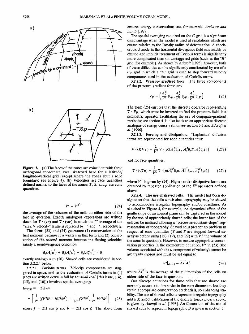
Figure 3. (a) The faces of the zones are coincident with three orthogonal coordinate axes, sketched here for a latitude/ longitude/vertical grid (except where the zones abut a solid boundary; see Figure 4). (b) Velocities are face quantities defined normal to the faces of the zones; T, S, and p are zone quantities.

V u = V •x (24) the average of the volumes of the cells on either side of the face in question. Exactly analogous expressions are written down for V ß (vv) and V ß (vw) in which the -x average of the "area x velocity" terms is replaced by -Y and -z, respectively.

The forms (23) and (24) guarantee (1) conservation of the first moment because it is written in flux form and (2) conservation of the second moment because the fluxing velocities satisfy a nondivergence condition

-x O x x x(Axøu ) + ) + z(Azøw ) = 0

exactly analogous to (20). Shaved cells are considered in section 3.2,2.4 below.

3.2.2.1. Coriolis terms. Velocity components are stag- gered in space, and so the evaluation of Coriolis terms in (1) (they are written down in full by Marshall et al. [this issue, (14), (15), and (16)]) involves spatial averaging:

Gcom = -2D,^v

[1 x l rvo•xy l vo•zZ ] = ffrø - bVz), , (25) where f = 2fl sin 4• and b = 211 cos •b. The above form

The form (26) ensures that the discrete operator representing V ß Vp, which must be inverted to find the pressure field, is a symmetric operator facilitating the use of conjugate-gradient methods; see section 4. It also leads to an appropriate discrete analogue of energy conservation; see section 3.3 and Adcroft et al. [1996].

3.2.2.3. Forcing and dissipation. "Laplacian" diffusion terms are represented for zone quantities thus:

1 (27a)

and for face quantities:

1 --x -•y --z V' (.Vu) = V' [.(Aj ø SxU. Az ø SjU)] (27b)

where l• is given by (24). Higher-order dissipative forms are obtained by repeated application of the V 2 operators defined above.

3.2.2.4. The use of shaved cells. The model has been de-

signed so that the cells which abut topography may be shaved to accommodate irregular topography and/or coastlines. As sketched in Figure 4, for example, the dynamical effect of the gentle slope of an abyssal plane can be captured in the model by the use of appropriately shaved cells; the lower face of the cell can be inclined allowing a "piecewise-constant-slope" representation of topography. Shaved cells present no Problem in respect of zone quantities (T and S are stepped forward exactly as before using (15), (19), and (22) with V ø the volume of the zone in question). However, to ensure appropriate conservation properties in the momentum equation, l• in (23) (the volume associated with the u component of velocity) cannot be arbitrarily chosen and must be set equal to

VUlshaved-- Ax•4x ø (28)

where Ax is the average of the x dimension of the cells on either side of the face in question.

Our discrete equations for those cells that are shaved are now only accurate to first order in the zone dimension, but they retain appropriate conservation credentials, so enhancing sta- bility. The use of shaved cells to represent irregular topography and a detailed justification of the discrete forms chosen above, is given by Adcroft et al. [1996]. An illustration of the use of shaved cells to represent topographic/3 is given in section 5.


v 0.

xzu A 0

/v o

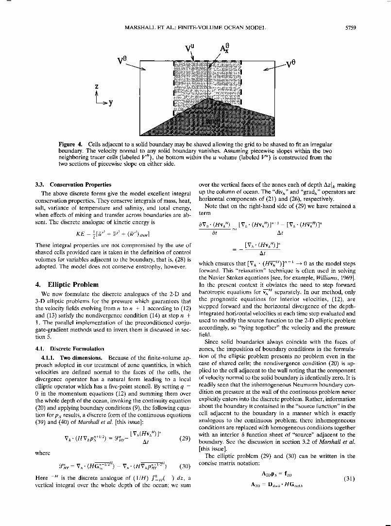
Figure 4. Cells adjacent to a solid boundary may be shaved allowing the grid to be shaved to fit an irregular boundary. The velocity normal to any solid boundary vanishes. Assuming piecewise slopes within the two neighboring tracer cells (labeled Vø), the bottom within the u volume (labeled V u) is constructed from the two sections of piecewise slope on either side.

3.3. Conservation Properties

The above discrete forms give the model excellent integral conservation properties. They conserve integrals of mass, heat, salt, variance of temperature and salinity, and total energy, when effects of mixing and transfer across boundaries are ab- sent. The discrete analogue of kinetic energy is

l

KE : • [ •x: + •: + ( •:) These integral properties are not compromised by the use of shaved cells provided care is taken in the definition of control volumes for variables adjacent to the boundary, that is, (28) is adopted. The model does not conserve enstrophy, however.

4. Elliptic Problem We now formulate the discrete analogues of the 2-D and

3-D elliptic problems for the pressure which guarantees that the velocity fields evolving from n to n + 1 according to (12) and (13) satisfy the nondivergence condition (14) at step n + 1. The parallel implementation of the preconditioned conjugate-gradient methods used to invert them is discussed in section 5.

4.1. Discrete Formulation

4.1.1. Two dimensions. Because of the finite-volume approach adopted in our treatment of zone quantities, in which velocities are defined normal to the faces of the cells, the divergence operator has a natural form leading to a local elliptic operator which has a five-point stencil. By setting q = 0 in the momentum equations (12) and summing them over the whole depth of the ocean, invoking the continuity equation (20) and applying boundary conditions (9), the following equation forps results, a discrete form of the continuous equations (39) and (40) of Marshall et al. [this issue]:

where

Vh' (HVhp• +1/2) = •f•-- [V•(H•S)] •

At (29)

•f•n• = Vh' (HG•f•/:% - Vh' (HV•p•7 •/'-•) (30) Here -r• is the discrete analogue of (I/H) fø_r• ( ) dz, a vertical integral over the whole depth of the ocean; we sum

over the vertical faces of the zones each of depth Azlk making up the column of ocean. The "diVh" and "gradh" operators are horizontal components of (21) and (26), respectively.

Note that on the right-hand side of (29) we have retained a

IVy. (H•)] "+•- IVy. (H•)]" at At

[Vh' (H•")]•

which ensures that [Vh ß (H•"] " 1 _• 0 as the model steps forward. This "relaxation" technique is often used in solving the Navier Stokes equations [see, for example, Williams, 1969]. In the present context it obviates the need to step forward barotropic equations for v-•"separately. In our method, only the prognostic equations for interior velocities, (12), are stepped forward and the horizontal divergence of the depth- integrated horizontal velocities at each time step evaluated and used to modify the source function to the 2-D elliptic problem accordingly, so "tying together" the velocity and the pressure field.

Since solid boundaries always coincide with the faces of zones, the imposition of boundary conditions in the formulation of the elliptic problem presents no problem even in the case of shaved cells; the nondivergence condition (20) is applied to the cell adjacent to the wall noting that the component of velocity normal to the solid boundary is identically zero. It is readily seen that the inhomogeneous Neumann boundary condition on pressure at the wall of the continuous problem never explicitly enters into the discrete problem. Rather, information about the boundary is contained in the "source function" in the cell adjacent to the boundary in a manner which is exactly analogous to the continuous problem; there inhomogeneous conditions are replaced with homogeneous conditions together with an interior 8 function sheet of "source" adjacent to the boundary. See the discussion in section 3.2 of Marshall et al. [this issue].

The elliptic problem (29) and (30) can be written in the concise matrix notation:

A2DpS = f2D

A2D = Ddivh'HGradh

term

0 V•' (H• s)


where A2D is a symmetric, positive-definite matrix (A2D has five diagonals corresponding to the coupling of the central point with surrounding points along the four "arms" of the horizontal V 2 Operator.) composed of Ddivh and Gradh (matrix repre- sentations of the "div" and "grad" operators), Ps is a column vector of surface pressure elements, and f2D is a column vector containing the elements of the right-hand side of (29). The system can thus be solved using a standard conjugate-gradient method, preconditioned for efficient solution on a parallel computer; see section 4.2. The attractively simple form (31) is a consequence of the finite-volume method employed and has considerable advantages over that which results in models which arrange the variables on a B grid. On the B grid a nine-point stencil is obtained and a difficulty arises because it contains a "null space" of "checkerboard" fields that are invis- ible to the operator. The operator A2D --- Ddivh ß HGradh does not contain this checkerboard null space. The difficulties of the B grid implementation are discussed at some length by Dukow- icz et al. [1993], where remedies are suggested and implemented.

In summary, then, the approach we have adopted has considerable advantages in regard to the pressure inversion. In particular, because (1) the divergence constraint on the evolving velocities is applied in integral form employing Gauss's theorem and (2) the kinematic boundary condition v- n = 0 (where n is a unit vector normal to a solid boundary) is applied at the face of a cell, then the form of (31) is unchanged, even if the face of a cell which abuts the solid boundary is inclined to coordinate surfaces. This property enables one to rather easily shave cells which abut boundaries to improve the representation of flow over topography.

4.1.2. Three dimensions. In nonhydrostatic calculations a three-dimensional elliptic equation must also be inverted for PNH to ensure that the local divergence vanishes. The appropriate discrete form can be deduced in a manner that exactly parallels that which was used to deduce (29). Taking the horizontal divergence of equation (12) and adding the vertical derivative of equation (13), invoking (14) and boundary conditions, the resulting elliptic equation can be written

A3DPNu= f3D (32)

A3D: Ddi v ß Grad

where A3r•, like A2D , is a symmetric, positive-definite matrix representing the discrete representation of V 2, but now in three dimensions. If the ocean column is made up of cells stacked up on top of one another which do not have equal heights Az, then A is not symmetric, but it can easily be sym- metrized by premultiplying it with a symmetrization matrix W, where

W •

Az 1 Az 2

Az N

In (32), f3r• and PNH are (1 x N) column vectors containing the source function (the discrete form of (444) and (44b) of Marshall et al. [this issue] and nonhydrostatic pressure, in each of the N = NxNyN z cells into which the ocean has been carved. The column vectors have singly subscripted elementspt in which the elements are first enumerated in each vertical

column and only then in the horizontal directions, thus

l=k+Nz(i- 1) + (NzXNx)(j- 1)

where i is an index increasing eastward, j is an index increasing southward, and k increases downward. Although huge, of size (NxNyNz) 2, A3r • has a particularly simple form which can be exploited to devise a highly efficient method of inversion.

A3r • has seven diagonals representing the coupling in the three space dimensions. In any particular row of the matrix the three leading diagonals, blocked into D i in (33) below, are the coefficients multiplying the pressure in the same vertical column of the ocean; the four diagonals in the wings, d, are the coefficients multiplying pressures in cells in the same horizontal plane. The matrix can usefully be blocked and arranged as shown below:

A3 D --

D• qd ß

qd D 2 qd

qd D3

qd ß ß

ß

ß

qd

qd D,

qd

qd

qd

qd ß ß qd DNxNy.

(33)

Here each block Di is a tridiagonal matrix representing 02/0 Z 2 and d is a diagonal matrix representing V•. The D and d are matrices of size Nz x Nz if there are N z zones in each column of the ocean: there are Nx x Nv such blocks, one for each column of the ocean.

One further property of A3r• should be noted. If the vertical dimension of a zone is much smaller than its horizontal extent

(as is often the case because the ocean is much shallower than it is wide), then the V32 • 02/0z 2 and A3D is dominated by the blocks D along its diagonal. The elements d are smaller than those of D by an amount (Az/Ax) 2. Moreover, the tracer parameter q always appears as a multiplier of the d matrix; see (33). Thus when q is set to zero (corresponding to the hydrostatic limit), A3r • is composed only of the blocks D and so can readily be inverted. Thus if we "precondition" (32) by premultiplying it by a matrix which is composed of the inverse of these blocks, that preconditioner will be an exact inverse of A3r• in the hydrostatic limit. These properties of A3r • will be exploited in our chosen method of solution.

4.2. Preconditioned Conjugate-Gradient Solution Method

Many standard references to preconditioned conjugate- gradient methods exist [see, for example, Press et al., 1986, and references therein], but for the sake of completeness we briefly give the "hub" of the method here, emphasizing the use we make of preconditioners. Our problem is to find p given A and f (see (31) and (32)), where

np= f (34)

and A is a symmetric, positive-definite matrix. In serious ocean modeling applications the size of A is too

large for direct methods to be possible in three dimensions and often in two dimensions too. Since A does not change in time, it could be inverted once and stored. However, although A is sparse, its inverse is dense and so operating with its inverse would involve N 2 multiplications, an unrealistic task given that typically N >> 100,000. So we adopt an iterative procedure, preconditioned conjugate-gradient iteration, which exploits


the sparseness of A and its diagonal dominance. The procedure involves repeated multiplication of the iterative solution by A and by another sparse matrix K, an approximate inverse of A; K is called the preconditioner.

The algorithm can be understood thus: Let us premultiply (34) by a (carefully chosen) matrix K, which is an approximate inverse of A, so that KA • I. Then (34) can be written

(I-C)p = Kf

where C = I - KA. To the extent that CI --> 0, the above suggests the following iterative scheme, where i is the iteration step:

where

pi+l= Cpi+ Kf

= p'+ b i

b i = Kr i

is called the "search direction" and

r'= f- Ap'

is the "residual vector." The r and b can be deduced from the

previous iteration using the relations

r '+l= r'- Ab'

b •+1 = Kr ,+1

r ø - f - Apø; b o _ Kpø

a• - [r', Kr'] -[b';Ab']

pm_ pi + aibi ;ri+• _ r i _ a•Ab I

bi+l _ Kr i+l q_ •ib i ,I, ?no

[ ' ] ,• yes

STOP

Figure 5. The preconditioned conjugate-gradient (PCG) algorithm. Here [ , ] is the inner product of two vectors.

in a procedure known as "Richardson iteration." The method can be accelerated by choosing search directions in an optimal way. Our chosen method, the conjugate-gradient method, selects search directions as linear combinations of the previous search direction (b i) and the current gradient (r' + •) modified by the preconditioner (K):

b '+• = Kr '+• + •b'

where •3 is a constant to be determined. The name "conjugate gradient" stems from the property that

[Ab i+•, b'] - 0; the search directions on consecutive iterations are conjugate to one another. Conjugate gradient also selects a parameter a to minimize the magnitude of the residual vector as measured by e-Ae, where, if there were no preconditioning, e = pi _ p ...... is the error vector in the direction of b i. Choosing the optimal values of a and •3 results in the algorithm shown in Figure 5.

The conjugate-gradient (CG) procedure involves, at each iteration, multiplication of vectors by A and K and the evaluation of two global sums to form the inner product. The cost of the preconditioner is one operation by it per iteration.

We have designed preconditioners, K, for both the 2-D and 3-D problems, so that (1) it can be easily stored, (2) the number of operations one has to perform when multiplying by it is as small as possible, and (3) it is a good approximation to A -• so the iterative procedure converges rapidly. Because the true inverse is dense, our choice will be a compromise between these, sometimes conflicting, ideal properties.

4.2.1. Two dimensions. At each horizontal location, (31) can be written

+ + + +

where the superscripts C, W, E, N, and S, denote the center, west, east, north, and south locations, respectively, in the operator's five-point stencil. The leading diagonal of A2D will be

composed of the a c and the four nonzero off diagonals will be composed of the a N's'E'w. Because of the dominance of the leading diagonal, to a first approximation,

pC a

One of the simplest forms that could be chosen for K2D, then, is to suppose that it is a diagonal matrix composed of elements equal to the reciprocal of the corresponding elements along the leading diagonal of A. However, this can be improved by constructing an approximate local inverse as follows.

At the five points in the stencil surrounding c then, to the same level of approximation, we may write

fw pW• ; pN• fN aC w a• etc. where denotes the point to the west, etc.

Hence we can make a better approximation to pC thus:

pC • 1 ( awfw aSfS aSfS a•f• To arrive at a symmetric preconditioner we replace a c[ w, etc., thus

a C 1 (a C c

giving, finally, our local preconditioner for use in Figure 5:

r c 2 ( a WrW a•r • Kmr•• • a c + ac w a + aC • a sFs a EFE + c c + (3S)

•though simple, (35) is highly effective, reducing the number


of iterations required for convergence by, typically, a factor of 4, and the computer time by a factor of 2.

4.2.2. Three dimensions. After considerable experimen- tation we have chosen a block-diagonal preconditioner, a matrix whose diagonal is made up of the inverse of the tridiagonal matrices D defined above:

K3D = ß D? 1 ß

D•x•Ny.

(36)

Evaluation of the inner products to compute a and/3 in Figure 5 involves forming the vector x, where

x=Kr

or, since K = D-•, where D is the matrix of diagonal elements of (33):

x = D-lr

If our ocean model has many levels, then D -• will be dense, and so storing and multiplying by D -• are also demanding of resources. Instead, we exploit the fact that D is tridiagonal and use "lower/upper" ("LU") decomposition to solve the preconditioning equations for x in the form

Dx --- r

We write D = LU where L is a lower triangular matrix and U an upper triangular matrix, which have the form

D •

dl el

e2

L •

ll

12

13

U _..

Ul hi

U2 h2

U3

It is easy to see that if li = ui, one can readily compute the elements of L and U thus:

U2 = x/d2- e•f•/d•; h2 ....

and so on.

Finding the inverse of D or solving problem Dx = r is then equivalent to solving the two sets of equations

tz=r

Ux=z (37)

first for z and then for x. This is straightforward because of the triangular structure of L and U. Importantly, the number of operations required to solve (37) for x scales as Nz compared to N2z if we had used the inverse of D directly.

The resulting preconditioner was found to be a good compromise; as we shall see in chosen examples in section 5, its use significantly reduces the number of iterations required to find a solution to (34) because it is an acceptable approximation to the inverse of A, it is sparse, and, most importantly, its application requires no communication across the network in the data-parallel implementation of the algorithm.

5. Parallel Implementation Three applications of the numerical algorithm to problems

of oceanographic interest (using HPE, QH, and NH) are described in the companion paper. Here we focus on the important numerical and computational issues. The algorithm outlined in the previous sections was developed and implemented on a 128-node CM-5, a massively parallel distributed-memory computer housed in the Laboratory for Computer Science at the Massachusetts Institute of Technology (MIT). The code was written in CMFortran, a data-parallel FORTRAN, closely related to High Performance Fortran (HPF). The data-parallel implementation can be thought of as a conventional sequential FORTRAN program augmented with array layout directives and data movement functions. There is a single thread of control which alternates between phases of local computation and global communication. The global communication can be regarded as the overhead of parallel execution, while the local computation is the actual work required by the algorithm. The parallel code distributes the model data across the local mem- ories of the CM5 processors using an approach which mini- mizes global communication yet, when it is required, facilitates communication using efficient data movement functions. The algorithm was also coded in an implicitly parallel language called Id, permitting a multithreaded implementation on MIT's data flow machine MONSOON. The programming issues are developed more fully by Arvind et al. (A comparison of implicitly parallel multi-threaded and data-parallel implementations of an ocean model based on the Navier Stokes

equations, submitted to Journal of Parallel and Distributed Computing) (hereinafter referred to as Arvind et al., submitted manuscript, 1996), in which the implicitly parallel multithreaded and data-parallel implementations are compared.

In deciding how to distribute the model domain over the available processors in the data-parallel approach, we had to bear in mind that the most costly task in our algorithm is finding the pressure field; a significant part of the computation is spent in the conjugate-gradient algorithms described in section 4. The principle steps involved there are the (repeated) application of the Laplacian (A) and preconditioning (K) operators and the forming of global sums. The A operator entails nearest-neighbor communication between adjacent zones in all three directions (white and black points in Figure 6). The preconditioner K3D connects zones only in a vertical line (black points only in Figure 6). Accordingly, in the data- parallel approach we decompose the domain into vertical columns that reach from the top to the bottom of the ocean. This


!

! !

Figure 6. Schematic diagram of an ocean geometry decom- posed into columns and distributed over 12 processors. The hypothetical domain shown here has a horizontal dimension of 32 x 18. The dotted lines indicate regions of the domain assigned to the same processor. The thin lines delineate the cells on each processor, eight cells in the x direction and six cells in the y direction. The open and solid dots define the stencils used in the PCG elliptic procedure.

ensures that vertically aligned cells in the model are resident on the same processor, so reducing communication.

Thus the computational domain is divided laterally into equally sized rectangles (see Figure 6). All the cells and associated faces contained within the volume of ocean underneath

the "tiles" are then ascribed to the same processor. The u faces and v faces at coordinates coincident with the edge of the rectangular region are assigned to the same processor as the cell to their east or north, respectively.

5.1. Pressure Inversion

In HPE and QH, our scheme's performance is comparable to conventional second-order finite difference hydrostatic codes. In typical applications the model has many vertical levels and most of the computer time is spent evaluating terms in the explicit time-stepping formulae; the work required to invert the 2-D elliptic problem for P s does not dominate. In

NH, however, the computational load can be significantly increased by the 3-D inversion required. One iteration of the three-dimensional elliptic solver demands of the order of 30 operations/cell, which is --•6% of the total arithmetic operation count of the explicit time-stepping routines. Therefore, if the 3-D inversion is not to dominate the prognostic integration, the preconditioned conjugate-gradient (PCG) procedure must converge in less than 15 or so iterations.

To be more specific, let us consider the pressure inversion in a zonally periodic channel as in the mixed layer calculation using NH presented in Plate 1 and Tables 1 and 2 of Marshall et al. [this issue]. There Nx = 200, N v = 119, and Nz = 19. The horizontal resolution is high (--•200 m), comparable to, but somewhat coarser than, the vertical resolution; the aspect ratio of the zones (/Xz//Xx) 2 = (0.2) 2, and so even in this config- uration which permits nonhydrostatic effects, the matrix A3r,, (33), is dominated by the blocks along its diagonal (33). With this in mind, let us evaluate and compare the effort required to invert (31) and (32), remembering that (32) is the overhead of the nonhydrostatic algorithm.

The accelerated convergence made possible by splitting the pressure field (16) is central to controlling the computational overhead of NH. Figure 7 shows the impact on the number of three-dimensional iterations, Ira, of solving separately for the pressure components. We plot Im (required to achieve a given residual accuracy e_•r)) as a surface. First, we find P s to a chosen accuracy e2r ) and then find P/VH, moving across the surface as indicated by the arrow. In order to control the divergence field an e3r) of-10-7 is required (e is defined in Figure 5) corresponding to a 3-D divergence in the velocity field of one part in 1012, sufficiently small to result in a stable prognostic integration. As e_,t) diminishes, the accuracy of P s increases and the number of 3-D iterations decreases dramat-

ically. We see that in the case where p is not separated into its component parts (or P s is not found sufficiently accurately), I_•D is several hundred, and the time spent in the 3-D inversion overwhelms the prognostic part of the algorithm. But if an accurate Ps is obtained first (i.e., e2r ) < 10 --•, in the flat "valley" in Figure 7), I3r • drops down to below 10. It should be remembered that in a hydrostatic calculation, P s must be

I3d

400

300

2OO

lOO

-10 -9 -8 -7 -6 -5 -4 -10 log S2d log S3d

Figure 7. Surface showing the number of 3-D iterations, I3r), required to achieve a given residual e3D. First, Ps is found in a 2-D inversion and then PNH is found in a 3-D inversion, moving across the surface in the direction of the arrow.


2000

1500

lOOO

500

>-. o

-500,

-lOOO-

-15oo.

"Beta"

-2000 0 2000 0

"Slope"

Figure 8. The pressure field in a numerical solution of a wind-driven homogenous ocean with one layer in the vertical. The basin is 2000 km wide. In Figure 8a a/3 plane is used and the depth of the ocean is kept constant; in Figure 8b an f plane is used and a topographic/3 effect equivalent to the/3 effect in Figure 8a is induced by appropriately shaving the cells.

found anyway and so the overhead of NH is now indeed man- ageable. Note the change in slope of the I3D surface indicates the drop in iteration count is due to accelerated convergence not a consequence of an improved initial guess.

Furthermore, in the hydrostatic limit, q = 0, our preconditioner inverts for P•vH in only one up-down sweep of the vertical column, because K3D is then the exact inverse of A3D. And even if q = 1, A3D will still be dominated by the blocks along its leading diagonal provided (Az/Ax) 2 << 1, and again, convergence is achieved very much more rapidly if we split the pressure field up and proceed as above.

Finally, it should be emphasized that the use of shaved cells to represent irregularities in the lower and lateral boundaries of our geometry (Figure 4) does not, in any way, complicate or compromise our inversion procedure for Ps or P•vH. All geo- metrical information is carried in the areas and volumes of the

cells. If shaved cells are used, the entries of A2D and A3D are changed accordingly, but they remain symmetric matrices. For example, Figure 8 compares two steady state solutions from our model using HPE illustrating the use of shaved cells to represent the slope of the ocean bottom in a homogenous ocean made up of only one layer of fluid. The solutions pertain to the wind-driven homogeneous ocean circulation theory of Stommel [1948] and followers; as in the analytical theory the model was configured with Cartesian geometry and driven by a highly idealized wind pattern.

On the left (Figure 8a) the ocean has a constant depth and there is a "/3 effect"; the Coriolis parameter varies linearly with y. On the right (Figure 8b), however, the Coriolis parameter is kept constant, but the cells are shaved in such a manner that the bottom slope thus created induces a "topographic/3 effect" which is exactly equivalent to the "planetary/3 effect" of Figure

8a; this example, together with many others is described in more detail in Adcroft et al. [1997]. The resulting solutions are virtually indistinguishable demonstrating the utility of our finite-volume approach in the representation of topography.

5.2. Parallel Performance

The algorithm maps efficiently to both multiprocessor and single-processor computers. The arithmetical operations required on the regular grid that connect points in the finite- volume discretization break down readily into many independent operations. These operations can then be easily distributed over many independent processors computing in parallel. Figure 9 charts the performance of our data-parallel code on the CM5 for a variety of problem sizes and for differ- ing numbers of processors. We see that for fixed problem size, there is a drop in efficiency as the number of processors goes up, due to communication overhead. The degree to which it drops reflects the finite time required to communicate information between processors. But at fixed granularity the efficiency remains constant, and the floating point throughput increases linearly with the number of processors. We see no sequential bottlenecks to prevent the algorithm scaling efficiently as computing architecture evolves. These issues are discussed in more detail by Arvind et al. (submitted manuscript, 1996).

6. Conclusions

We have outlined the numerical implementation of an ocean model rooted in the Navier Stokes equations. This kernel algorithm can be readily modified to yield hydrostatic and quasi- hydrostatic forms. The spatial discretization employs finite- volume techniques permitting one to shave cells adjacent to the boundary and so accommodate geometries as complex as those of ocean basins with minimal increase in algorithmic complexity.

In the Navier Stokes model the pressure field, which ensures that evolving currents remain nondivergent, is found by inversion of a three-dimensional elliptic operator subject to Neu-

lOO

95

• 85

80

75

_ _ 13.15 Gflop/sec

_0

-

-

I [] Fixed problem size (512 x 256 x 20) 1 •

• I ß Fixed granularity size (32 x 32 x 20) I •X• lO.3S afop/s

;•2 1•4 1•8 2,•6 5'{2 No. CM-5 Nodes

Figure 9. Variation of model parallel efficiency, E, with processor count where E = 32T[32]/(nT[n]), the speed of the algorithm running on n processors compared to the speed on 32 processors.


mann boundary conditions. Preconditioned conjugate gradient iteration is used. A major objective has been to make this inversion, and hence nonhydrostatic modeling, efficient. By separating the pressure intops, Pn, andPNn components and carefully preconditioning the resulting coupled 2-D and 3-D elliptic equations, a simple and indeed efficient algorithm results. Moreover, the algorithm smoothly moves from hydrostatic to nonhydrostatic limits; in the hydrostatic limit, our NH algorithm (even though it is prognostic in w) is exactly equivalent to, and no more demanding of computer resources than, a hydrostatic model. But, unlike a hydrostatic model, as the resolution of NH is increased, it can be used to address small- scale phenomena which are not hydrostatically balanced. Even in experiments of resolved convection using NH where nonhydrostatic effects play a central role, separation of the pressure field into its component parts leads to great savings.

The approach maps naturally onto a parallel computer and suggests a domain decomposition which allocates entire vertical columns of the ocean to each processing unit. The resulting model is efficient and scalable and suitable for the study of the ocean circulation on horizontal scales less than the depth of the ocean, right up to global scale.

The possible applications of such a model are myriad. In the hydrostatic limit it can be used in a conventional way to study the general circulation of the ocean in complex geometries. But because the algorithm is rooted in NH, it can also address (for example) (1) small-scale processes in the ocean such as convection in the mixed layer, (2) the scale at which the hydrostatic approximation breaks down, and (3) questions con- cerning the posedness of the hydrostatic approximation raised by, for example, Browning et al. [1990] and Mahadevan et al. [1996a, b]. Finally, it is interesting to note that, as described by Brugge et al. [1991], the incompressible Navier Stokes equations developed here are the basis of the pressure-coordinate quasi-hydrostatic atmospheric convection models developed by Miller [1974]. Thus the ocean model described here is isomor- phic to atmospheric forms, suggesting that it could be developed and coupled to a sibling atmospheric model based on the same numerical formulation.

z - 0 is much less than the local depth of the ocean. Then we may write

Oh --+ Vh' H•hh H= 0 ot

where the-n is defined after (30). The •hh n evolves according to the momentum equations,

obtained by vertically integrating (12):

O•hh H H O•- + gVhh = Rvh

where the hydrostatic relation has been used to relate the surface pressure Ps at z = 0 to the perturbation h about z - 0 and R is the vertical integral of G over the water column less the vertical integral of interior hydrostatic pressure gradients.

Implicit discrete forms of these relations are

hn+l __ h n

At + Vh' [H•hhH] n+•= 0 (A1)

At + •]Vh hn+l: [RvhH] n+l/2 (A2)

Multiplying (A2) by H, taking its horizontal divergence, and using (A1) lead to the following Helmholtz equation'

h "+• i h •' ' - - Vh' [HR•"]• + •7 h [HVh h"•] gat 2- g gat 2

+ gat (A3) Note that (A3) is better conditioned for inversion than (29) because the 1/( gat 2) term results in an A2D matrix of greater diagonal dominance than that used to represent the left-hand side of (29), greater by an amount [1 + (Ax2/c2At2)), where c = X/gH is the external gravity wave speed and Ax is a measure of the lateral dimensions of the cells. If the distance

traveled by the eternal gravity wave in one time step is only a few Ax, then (A3) will converge rapidly.

Appendix 1 In spherical coordinates, zones are defined by intersecting

surfaces every (A/X, zX&, zXr) of (longitude, latitude, height), and (except when they abut irregular topography) the volumes of the zones and the surface areas of their faces are given by

/t• •: rA&Ar; Ay ø = r cos &A/XAr; A• ø = r 2 COS &A&A/•

I/ø= r 2 COS qbAqbAXAr

Analogous expressions can be written down in other coordinate systems.

Appendix 2: Implicit Free Surface The rigid-lid condition can be readily relaxed and the surface

of the model ocean treated as a free surface. If implicit methods are used [e.g., Dukowicz and Smith, 1994], the same time step can be employed as for all other model variables. More- over, the resulting modified 2-D elliptic equation forps is more easily inverted.

Let us suppose that the elevation of the free surface h about

Acknowledgments. This research was supported by grants from ARPA, TEPCO, and the Office of Naval Research. The model was developed on the CM5 housed in the Laboratory for Computer Sci- ence (LCS) at MIT as part of the SCOUT initiative. Much advice and encouragement on computer science aspects of the project was given by Arvind of LCS. Jacob White of the Department of Electrical En- gineering and Computer Science at MIT advised on the solution of elliptic problems on parallel computers. We have often consulted Andy White of the UK Meteorological Office and our colleague Jo- chem Marotzke on the mathematical and numerical formulation of the ocean model.

References

Adcroft, A., Numerical algorithms for use in a dynamical model of the ocean, Ph.D. thesis, Imp. Coil., London, 1995.

Adcroft, A., C. Hill, and J. Marshall, Treatment of topography in ocean models using finite-volumes, Mon. Weather Rev., in press, 1997.

Arakawa, A., and V. Lamb, Computational design of the basic dynamical processes of the UCLA General Circulation Model, Methods Cornput. Phys., 17, 174-267, 1977.

Bleck, R., and L. Smith, A wind-driven isopycnic coordinate model of the North and equatorial Atlantic Ocean, 1, Model development and supporting experiments, J. Geophys. Res., 95(C3), 3273-3285, 1990.


Browning, G. L., W. R. Holland, H.-O. Kreiss, and S. J. Worley, An accurate hyperbolic system for approximately hydrostatic and incompressible flows, Dyn. Atmos. Oceans, 14, 303-332, 1990.

Brugge, R., H. L. Jones, and J. C. Marshall, Non-hydrostatic ocean modeling for studies of open-ocean deep convection, in Deep Con- vection and Deep Water Formation in the Oceans, Elsevier Oceanogr. Set., vol. 57, pp. 325-340, Elsevier Sci., New York, 1991.

Clarke, T., A small-scale dynamical model using a terrain-following coordinate transformation, J. Cornput. Phys., 24, 186-215, 1977.

Dukowicz, J. K., and A. S. Dvinsky, Approximate factorization as a high order splitting for the implicit incompressible flow equations, J. Cornput. Phys., 102, 336-347, 1992.

Dukowicz, J. K., and R. D. Smith, Implicit free surface for the Cox- Bryan-Semtner ocean model, J. Geophys. Res., 99(C4), 7991-8014, 1994.

Dukowicz, J. K., R. D. Smith, and R. C. Malone, A reformulation and implementation of the Bryan-Cox-Semtner ocean model on the connection machine, J. Atmos. Oceanic Technol., 10, 195-208, 1993.

Flosadottir, A. H., J. C. Larsen, and J. T. Smith, The relation of sea-floor voltages to ocean transports in North Atlantic Circulation models; model results and practical considerations for transport monitoring, J. Phys. Oceanogr., in press, 1996.

Haidvogel, D. B., J. L. Wilkin, and R. Young, A semi-spectral primitive equation ocean circulation model using sigma and orthogonal cur- vilinear coordinates, J. Cornput. Phys., 94, 151-185, 1991.

Haney, R. L., On the pressure gradient force over steep topography in sigma coordinate ocean models, J. Phys. Oceanogr., 21, 610-619, 1991.

Harlow, F. H., and J. E. Welch, Time depended viscous flow, Phys. Fluids, 8, 2182-2193, 1965.

Mahadevan, A., J. Oliger, and R. Street, A non-hydrostatic mesoscale ocean basin model, I, Well-posedness and scaling, J. Phys. Oceanogr., in press, 1996a.

Mahadevan, A., J. Oliger, and R. Street, A non-hydrostatic mesoscale

ocean model, II, Numerical implementation, J. Phys. Oceanogr., in press, 1996b.

Marshall, J., C. Hill, L. Perelman, and A. Adcroft, Hydrostatic, quasi- hydrostatic, and nonhydrostatic ocean modeling, J. Geophys. Res., this issue.

McCalpin, J. D., A comparison of second-order and fourth-order pressure gradient algorithms in a (r-coordinate ocean model, Int. J. Numer. Methods Fluids, •8(4), 361-383, 1994.

Mellor, G. L., Users Guide for a Three-Dimensional, Primitive Equation, Numerical Ocean Model, Princeton Univ., Princeton, N.J., 1992.

Miller, M. J., On the use of pressure as vertical coordinate in modeling convection, Q. J. R. Meteorol. Soc., 100, 155-162, 1974.

Potter, D., Computational Physics, John Wiley, New York, 1976. Press, W. H., B. P. Flannery, S. A. Teukolsky, and W. T. Vettering,

Numerical Recipes, Cambridge Univ. Press, New York, 1986. Stommel, H., The westward intensification of wind-driven ocean cur-

rents, Eos Trans. AGU, 29(2), 202-206, 1948. Tanguay, M., and A. Robert, Elimination of the Helmholtz Equation

associated with the semi-implicit scheme in a grid-point model of the shallow water equations, Mon. Weather Rev., 114, 2154-2162, 1986.

Williams, G. P., Numerical integration of the three-dimensional Navier Stokes equations for incompressible flow, J. Fluid Mech., 37, 727-750, 1969.

A. Adcroft, C. Heisey, C. Hill, J. Marshall, and L. Perelman, Center for Meteorology and Physical Oceanography, Department of Earth, Atmospheric and Planetary Sciences, Massachusetts Institute of Tech- nology, Building 54, Room 1526, Cambridge, MA 02139. (e-mail: marshall @gulf. mit.edu)

(Received August 31, 1995; revised July 31, 1996; accepted August 21, 1996.)

a finite-volume, incompressible navier stokes model for...

Documents