a fourier approach for nonlinear equations with singular data
TRANSCRIPT

ISRAEL JOURNAL OF MATHEMATICS 193 (2013), 83–107
DOI: 10.1007/s11856-012-0032-1
A FOURIER APPROACHFOR NONLINEAR EQUATIONS WITH SINGULAR DATA
BY
Lucas C. F. Ferreira and Marcelo Montenegro
Universidade Estadual de Campinas, IMECC–Departamento de Matematica
Rua Sergio Buarque de Holanda, 651, Campinas-SP, Brazil, CEP 13083-859
e-mail: [email protected] and [email protected]
ABSTRACT
For 0 < m < n, p a positive integer and p > n/(n − m), we study the
inhomogeneous equation Lu+up + V (x)u+ f(x) = 0 in Rn with singular
data f and V. The symbol σ of the operator L is bounded from below
by |ξ|m. Examples of L are Laplacian, biharmonic and fractional order
operators. Here f and V can have infinite singular points, change sign,
oscillate at infinity, and be measures. Also, f and V can blow up on an
unbounded (n−1)-manifold. The solution u can change sign, be nonradial
and singular. If σ, f and V are radial, then u is radial. The assumptions
on f and V are in terms of their Fourier transforms and we provide some
examples.
1. Introduction
In this paper we study the following inhomogeneous equation,
(1.1) L(u) + up + V (x)u + f(x) = 0 in Rn,
where the multiplier operator L(·) is defined by
Lu = σ(ξ)u,
with g =∫
Rn g(x)e−2πix·ξdξ standing for the Fourier Transform of g. Through-
out this paper 0 < m < n, p ∈ N, p > n/(n−m) and the symbol σ satisfies
(1.2)1
|σ(ξ)| ≤M|ξ|m for a.e. ξ ∈ R
n, where M is a constant.
Received November 9, 2010
83

84 L. C. F. FERREIRA AND M. MONTENEGRO Isr. J. Math.
Examples of L are Laplacian, biharmonic and fractional order operators. El-
liptic equations with singular potential emerge naturally in many physical sit-
uations; see [4, 7, 8, 11, 13] and references therein. Our main aim is to study
(1.1) by means of a Fourier approach which allows us to consider a larger class
of singular potentials V and forcing terms f .
Usually, the Fourier Transform is a powerful tool to solve linear partial differ-
ential equations, because the resulting algebraic equation can be solved for u.
And by inversion, u∨ turns out to be a solution of the original equation. In this
paper we intend to carry out a resembling strategy for a nonlinear equation and
the corresponding nonalgebraic equation in Fourier variables. For that matter,
we formulate (1.1) in the following functional equation,
(1.3) u = N(u) + TV (u) + F (f),
where the operators B(u), TV (u) and F (f) are defined by means of a Fourier
Transform:
N(u) ≡ − 1
σ(ξ)(u ∗ u ∗ · · · ∗ u)︸ ︷︷ ︸
p-times
,(1.4)
TV (u) ≡ − 1
σ(ξ)(V ∗ u) and F (f) ≡ − 1
σ(ξ)f .(1.5)
The notation ∗ stands for the convolution product and u ∗ u ∗ · · · ∗ u has p-
factors. As we shall see, the assumptions on f and V are in terms of their
Fourier Transforms. The environment where we will study (1.3), (1.4) and
(1.5) is described in the sequel. Denote the Schwartz space S(Rn) of functions
decaying more rapidly than any polynomial and S ′(Rn) the space of tempered
distributions. An adequate space to deal with equation (1.3) is the following
one:
(1.6) Sa ≡{
v ∈ S ′(Rn) : v ∈ L1loc(R
n), supξ∈Rn
|ξ|a|v(ξ)| <∞}
with norm given by
‖v‖Sa = supξ∈Rn
|ξ|a|v(ξ)|.
Standard examples we will work with are V (x) = 1/|x|m in Sn−m and f(x) =
1/|x|mp/(p−1) in Sn−mp/(p−1) or linear combinations of translations of such V
and f ; more examples will be presented in Section 2. The casem = 2 has special
interest and corresponds to Laplacian operator and multisingular inverse-square

Vol. 193, 2013 FOURIER APPROACH FOR NONLINEAR EQUATIONS 85
potentials (see, e.g., [4] and references therein). The Banach space Sa fits one
of our needs, since when applying a Fourier Transform in equation (1.1), the
operator L(·) gives rise to a possible singular term 1/|ξ|m in the right-hand side
of the equation. Space Sa is also useful to deal with convolutions and have been
used to prove existence of solutions in fluid mechanics; see [6] and references
therein.
In some special cases, the solutions we are going to seek are scaling in-
variant. That is, they are homogeneous with singularity at the origin (i.e.,
lim sup|x|→0 |u(x)| = ∞), and therefore do not belong to any Sobolev space. To
be more precise, assume that the symbol σ(ξ) is homogeneous of degree m and
that u is a smooth solution of (1.1). Denoting Vλ(x) = λmV (λx) and fλ(x) =
λmp/(p−1)f(λx), it is easy to check that, for all λ > 0, uλ(x) = λm/(p−1)u(λx) is
also a smooth solution of (1.1) with V and f replaced by Vλ and fλ, respectively.
Consider the scaling
(1.7) u→ uλ = λm/(p−1)u(λx).
Replacing λ > 0 by λ−1 > 0, we can express (1.7) in terms of Fourier variables,
namely
(1.8) u→ (uλ−1)ˆ = λn−m/(p−1)u(λξ).
The solutions are scaling invariant by (1.7) (or (1.8)) when they are homo-
geneous of degree −m/(p − 1) or, equivalently, their Fourier Transforms are
−(n−m/(p− 1))-homogeneous. Observe that a = n−m/(p− 1) is the unique
exponent such that ‖u‖Sa = ‖uλ‖Sa for all λ > 0, i.e., the norm ‖ · ‖Sa is
invariant by scaling (1.7).
In Theorem 1.1 (i) we obtain a solution to the functional equation (1.3). In
general, a solution u ∈ Sa of (1.3) does not have enough regularity to satisfy
(1.1) even in the sense of distributions. One of the difficulties to regularize it
relies on the p-product of convolutions and V ∗ u and the singular factor 1/|ξ|mat the origin; see (1.4) and (1.5). With more structure, part (ii) shows that the
solution u of (1.3) belongs to some Lq. In part (iii) we work in the space H1,s,
defined in (1.10), of functions which are not singular. Moreover, a function in
H1,s is continuous and decays to 0 at ∞. We show in part (iii) that in fact u is a
classical solution of (1.1), belongs to C [m+s](Rn) and decays to 0 at ∞. Notice
that L is invariant by rotations if and only if σ is radial. In this respect, in
Theorem 1.2 we address the radial symmetry and homogeneity of the solution,

86 L. C. F. FERREIRA AND M. MONTENEGRO Isr. J. Math.
respectively in items (i) and (ii). Other methods were applied in [10] to study
radial symmetry in case L(u) = −(−Δ)m/2u and f ≡ 0. By using that radial
and homogeneous functions have the form const/|x|k, in Theorem 1.2 (iii) we
find a solution with nonremovable singularity at 0 satisfying equation (1.1) in
Rn−{0}. This is a peculiar fact due to the symmetry and homogeneity, since in
general one knows only that the solution u belongs to Sa with a = n−m/(p−1).
Notice that n/2 < a < n, then u ∈ L1+L2, and hence u ∈ L∞+L2. Therefore,
in general, we cannot assure the equality (u ∗ u ∗ · · · ∗ u)∨ = up, unless we
assume further properties; see Theorem 1.1 (iii). Differently, for solutions u of
the form const/|x|k, the p-product of convolutions satisfies (u∗ u∗· · ·∗ u)∨ = up.
In Theorem 1.3 we show an asymptotic stability ensuring that some types of
perturbations of f and V are negligible for large harmonics |ξ|.Elliptic equations with L(u) = Δu and a smooth bounded potential V decay-
ing to 0 at ∞ have been treated in [17] by variational methods. An equation
involving L(u) = Δ2u with bounded potential tending to a positive constant
at ∞ was considered in [3]. We can also deal with a potential featuring such
behavior; see Example 2.6. Specifically, equation Δu + up + f(x) = 0 with f
smooth and p > n/(n − 2) was studied in [1, 2, 12] by a sub-super-solution
method. Analogous results for Δ2u + up + f(x) = 0 have been obtained in
[16] for p > n/(n − 4). In particular, we may take 1 < p ≤ n/(n − 2) if m is
small enough, which happens with a fractional differential operator with small
order. Linked to an α-stable process, the case L(u) = −(−Δ)α2 u and V ≡ 0
was studied in [14] with f bounded, smooth and having compact support. In
our results, f and V can oscillate (but non-periodically) at ∞, change sign, be
nonradial and carry infinite singularities, that is, they can blow-up on an un-
countable number of points and also in an unbounded (n− 1)-manifold in Rn;
see Examples 2.1–2.4 in Section 2. In Example 2.5 we address the case where
f and V are measures concentrated on a submanifold of Rn.
Since f and V belong to some space Sd, then f and V decay polynomially,
but not necessarily f and V , because the Fourier Transform operator is not
monotone. In fact, f and V can oscillate and be unbounded at ∞; see Examples
2.3 and 2.4 in Section 2.
We denote
(1.9) Ck0 (R
n) = {v ∈ Ck(Rn) : ∂αv vanish at ∞, for all |α| ≤ k}and
(1.10) H1,s = {v ∈ S ′(Rn) : (1 + |ξ|s) v ∈ L1(Rn)} ⊂ C0(Rn),

Vol. 193, 2013 FOURIER APPROACH FOR NONLINEAR EQUATIONS 87
endowed with norm ‖v‖1,s = ‖(1 + |ξ|s)v‖L1 .
We are ready to state the existence result of solutions for (1.1).
Theorem 1.1: Let 0 < m < n, p ∈ N, p > n/(n − m), a = n − m/(p − 1),
f ∈ Sa−m and V ∈ Sn−m.
(i) (Existence and uniqueness) Let
τa = La‖V ‖Sn−m and εa = (1 − τa)p/(p−1)/(2pKa)
1/(p−1)
where the constantsKa and La are as in Lemma 3.3 below. If ‖V ‖Sn−m<
1/La and ‖f‖Sa−m ≤ ε/M with 0 < ε < εa, then equation (1.3)
has a unique solution u such that ‖u‖Sa ≤ 2ε/(1− τa). Moreover,
u ∈ L∞ + L2 (and u is a function).
(ii) (Further decay) Assume that f ∈ Sa−m ∩ Sb−m with m < b < n and
‖V ‖Sn−m < 1/Lb. There exists 0 < δb ≤ ε such that if ‖f‖Sa−m ≤δb/M, then the previous solution u belongs to Sa ∩ Sb. Moreover, if
b > a then u ∈ Lq for all n/(n− a) < q < n/(n− b). In case b < a we
have u ∈ Lq for all n/(n− b) < q < n/(n− a).
(iii) (Regularity) Let s ≥ 0 and the constants L1,s, ˜La,s be as in Lemma
3.4. Assume that f, V ∈ H1,s with
τ = max{L1,s‖V ‖1,s, (˜La,s + La)‖V ‖Sn−m} < 1.
There exists 0 < ε ≤ ε such that if
(1.11) ‖f‖Sa−m
{[p− 1
mpR
mpp−1 +
(p− 1
mp+ s)
Rmpp−1+s
]
area(Sn−1) + 1}
+1
|R|m∫
|ξ|>R
| f |dξ ≤ ε
M ,
for some R > 0, then the solution u ∈ C[m+s]0 (Rn) and satisfies (1.1)
in a classical sense. Here [s] stands for the greatest integer less than or
equal to s.
To proceed further, we recall some basic concepts about tempered distribu-
tions. A distribution u is called homogeneous of degree h if
〈u, ϕ(x/λ)〉 = λn+h〈u, ϕ(x)〉 for all λ > 0 and ϕ ∈ S(Rn).
Also, u is radial if it verifies
〈u, ϕ(T (x))〉 = 〈u, ϕ(x)〉 for all rotations T and ϕ ∈ S(Rn).

88 L. C. F. FERREIRA AND M. MONTENEGRO Isr. J. Math.
These properties are the content of the next result.
Theorem 1.2: Let u be the solution corresponding to f and V obtained in
Theorem 1.1 part (i).
(i) (Radial symmetry) Assume that the symbol σ(ξ) is radial. The solution
u is radial if f and V are radial. If f is nonradial and V is radial, then
u is nonradial.
(ii) (Scaling invariant solutions) Let σ(ξ) be a homogeneous function of
degree m. Assume that f and V are homogeneous distributions of
degrees −mp/(p− 1) and −m, respectively. Then u is a homogeneous
function of degree −m/(p− 1) (can be nonradial), i.e.,
u(x) = λm/(p−1)u(λx), a.e. x ∈ Rn and λ > 0.
In particular, lim sup|x|→0 |u(x)| = ∞.
(iii) Assume the hypotheses of item (ii) and that σ(ξ) is radial. If f and V
are radial, then u ∈ C∞(Rn − {0}) and u satisfies (1.1) in the classical
sense in Rn − {0}. In particular, |u(x)| → ∞ as |x| → 0.
In the sequel we state the asymptotic stability result.
Theorem 1.3: Let u1 and u2 be solutions of (1.3) obtained in Theorem 1.1,
corresponding to f1, V1 and f2, V2 with m < b < n and fi ∈ Sa−m ∩ Sb−m,
i = 1, 2. If
(1.12) lim|ξ|→0
|ξ|b−m|f1(ξ)− f2(ξ)| = 0 and lim|ξ|→0
|ξ|m|V1(ξ)− V2(ξ)| = 0,
then
(1.13) lim|ξ|→0
|ξ|b|u1(ξ)− u2(ξ)| = 0.
If
(1.14) lim|ξ|→∞
|ξ|b−m|f1(ξ)− f2(ξ)| = 0 and lim|ξ|→∞
|ξ|m|V1(ξ) − V2(ξ)| = 0,
then
(1.15) lim|ξ|→∞
|ξ|b|u1(ξ)− u2(ξ)| = 0.
Remark 1.4: Notice that the solutions given by item (i) of Theorem 1.1 sat-
isfy u = O(|ξ|−a) provided that f = O(|ξ|−(a−m)) and V = O(|ξ|−(n−m)) as
|ξ| → ∞. In particular, Theorem 1.3 refines the latter assertion, in the sense

Vol. 193, 2013 FOURIER APPROACH FOR NONLINEAR EQUATIONS 89
that u = o(|ξ|−a) provided that f = o(|ξ|−(a−m)) and V = o(|ξ|−(n−m)) as
|ξ| → ∞. In fact, in this case one has
(1.16) lim|ξ|→∞
|ξ|a−m|f(ξ)| = 0 and lim|ξ|→∞
|ξ|n−m|V (ξ)| = 0,
and, applying Theorem 1.3, with a = b, u2 = V2 = f2 = 0, u = u1, V = V1 and
f = f1, we obtain
(1.17) lim|ξ|→∞
|ξ|a|u(ξ)| = 0.
Notice that (1.16) holds, for instance, when f ∈ S(Rn)‖·‖Sa−m and V ∈
S(Rn)‖·‖Sn−m . The same conclusions hold true if one replaces |ξ| → ∞ by
|ξ| → 0.
Remark 1.5: In case V1 = V2 = V , a slight adaptation of the proof of Theorem
1.3 shows that the converse holds true. That is, (1.13) and (1.15) imply (1.12)
and (1.14), respectively.
2. Examples
Example 2.1 (Infinite singular points): Theorem 1.1 part (i) allows us to con-
sider potentials V and inhomogeneous terms f with infinite singularities, that
is, blowing up (i.e., tending to ±∞) at an infinite number of points. For in-
stance, let {Vj}∞j=1 be homogeneous functions of degree −m, {μj}∞j=1 satisfying
Σ∞j=1 |μj | ‖Vj‖Sn−m <∞, {xj}∞j=1 ⊂ R
n such that xk �= xj when k �= j and let
V (x) =
∞∑
j=1
μjVj(x− xj).
Notice that |V (xj)| → ∞ as x→ xj , for all j, and if |xj | → ∞ as j → ∞, then
lim sup|x|→∞
|V (x)| = ∞.
We have V ∈ Sn−m because
∣
∣
∣V (ξ)∣
∣
∣ =
∣
∣
∣
∣
∞∑
j=1
μj Vj(ξ)e−2πiξ·xj
∣
∣
∣
∣
≤ (
Σ∞j=1 |μj | ‖Vj‖Sn−m
) 1
|ξ|n−m for all ξ ∈ Rn.

90 L. C. F. FERREIRA AND M. MONTENEGRO Isr. J. Math.
Similarly, one can take f =∑∞
j=1 μjfj(x− xj) with fj homogeneous of degree
−mp/(p− 1).
Example 2.2 (Blow-up on a compact (n − 1)-manifold): We are able to deal
with f and V tending to ±∞ on a (n− 1)-manifold. Let r > 0 and Mλ,r(x) be
defined by
(2.1) Mλ,r(x) =
⎧
⎨
⎩
(r2 − |x|2)λ if |x| ≤ r,
0 if |x| > r.
Notice that Mλ,r(x) = r2λMλ,1(x/r) blows-up on |x| = r provided that λ < 0.
For each λ > −1, we have an explicit expression for Mλ,r (see [9, p. A-10]):
Mλ,r(ξ) = rn+2λMλ,1(rξ) = rn+2λΓ(λ+ 1)
πλ
Jn2 +λ(2π |rξ|)|rξ| n2 +λ
where Γ(z) is the Gamma function and Jk(s) the Bessel function of order k. By
the asymptotic forms of Jk(z), there exists a constant Qn,λ depending only on
n, λ such that∣
∣
∣Mλ,r(ξ)∣
∣
∣ ≤ Qn,λrn+2λ
(1 + r |ξ|)n+12 +λ
.
Thus, for 0 ≤ d ≤ n+12 + λ, we have that Mλ,r ∈ Sd because
(2.2)
‖Mλ,r‖Sd= sup
ξ∈Rn
|ξ|d∣
∣
∣Mλ,r(ξ)∣
∣
∣ = r−d supξ∈Rn
|rξ|d∣
∣
∣Mλ,r(ξ)∣
∣
∣
≤ Qn,λrn+2λ−d sup
ξ∈Rn
|rξ|d 1
(1 + |rξ|)n+12 +λ
≤ Qn,λrn+2λ−d.
In case n < 2m+ 1, observe that there is −1 < λ < 0 such that 0 < a −m <
n −m ≤ n+12 + λ. Therefore, in Theorem 1.1 (i) one can take V ∈ Sn−m and
f ∈ Sa−m in the form (2.1) times a small constant and with λ < 0. To obtain
f and V tending to −∞; consider −Mλ,r(x). In fact, we can consider a linear
combination of functions in the form Mλ,r(x).
Next we consider an infinite linear combination of translations of functions
Mλ,r(x).

Vol. 193, 2013 FOURIER APPROACH FOR NONLINEAR EQUATIONS 91
Example 2.3 (Blow-up on an unbounded manifold and Oscillation): Let rj > 0,
xj ∈ Rn, μj ∈ R and
(2.3) G(x) =
∞∑
j=1
μjMλ,rj (x− xj).
By (2.1) and (2.2), we have
‖Mλ,rj(x− xj)‖Sd= ‖Mλ,r‖Sd
≤ Qn,λrn+2λ−dj ,
for all j and 0 ≤ d ≤ (n+ 1)/2 + λ. If Σ∞j=1 |μj | rn+2λ−d
j < ∞, then G ∈ Sd
with
‖G‖Sd≤
∞∑
j=1
|μj | ‖Mλ,rj (x− xj)‖Sd≤ Qn,λ
∞∑
j=1
|μj | rn+2λ−dj <∞.
In particular, taking μj = (−1)jj, rj = j−3/(n+2λ−d) and |xj | → ∞, notice
that G(x) blows-up on an unbounded manifold and G(x) oscillates as |x| → ∞.
Also, G(x) is unbounded from below and above as |x| → ∞. In case n < 2m+1,
there is −1 < λ < 0 such that 0 < a−m < n−m < (n+ 1)/2 + λ, and so one
can take V and f as in (2.3).
Example 2.4 (Oscillation at ∞ in all directions): Now we construct f and V
oscillating in all directions. Denote Ar = {x ∈ Rn : |x| ≤ r} and, by (2.1), note
that 1Ar ≡Mλ,r when λ = 0. From (2.1) and (2.2) we have
(2.4) 1Ar(ξ) = rn/2Jn/2(2πr |ξ|)
|ξ|n/2.
Consider the family of rings Wj = {x ∈ Rn : rj < |x| ≤ rj + δj} and
(2.5) G(x) =
∞∑
j=1
μj1Wj (x),

92 L. C. F. FERREIRA AND M. MONTENEGRO Isr. J. Math.
where μj ∈ R. Recall the following Bessel function property: φ′k(z) = zkJk−1(z)
where φk(z) = zkJk(z). The Mean Value Theorem and (2.4) yield
∣
∣
∣
1Wj (ξ)∣
∣
∣ =∣
∣
∣
(
1Arj+δj(ξ)− 1Arj
(ξ))∣
∣
∣
= |ξ|−n/2∣
∣
∣
(
(rj + δj)n/2Jn/2 (2π(rj + δj) |ξ|)− r
n/2j Jn/2(2πrj |ξ|)
)∣
∣
∣
= (2π)−n/2 |ξ|−n ∣∣
(
φn/2(2π |ξ| (rj + δj))− φn/2(2π |ξ| rj))∣
∣
= (2π)−n/2 |ξ|−n∣
∣
∣φ′n/2(2π |ξ| (rj + δj))δj
∣
∣
∣
= (2π(rj + δj))n/2(2π |ξ| (rj + δj))
−n/2∣
∣
∣Jn−22(2π |ξ| (rj + δj))
∣
∣
∣ δj
≤ C
(
1A1
(rj + δj)n/2−1δj
|ξ| + 1AC1
(rj + δj)−3/2δj
|ξ|(n+1)/2
)
,(2.6)
where 0 < δj < δj for all j. In the latter inequality we used the asymptotic
form of Jk from [9, p. A-11]. Assuming 1 ≤ d ≤ (n+ 1)/2, the estimate (2.6)
implies
supξ∈Rn
|ξ|d∣
∣
∣
1Wj (ξ)∣
∣
∣ ≤ Qn
(
(rj + δj)n/2−1 + rj
−3/2)
δj
:= ψ(rj , δj).
Thus G ∈ Sd with
(2.7) ‖G‖Sd≤
∞∑
j=1
|μj | ‖1Wj‖Sd≤
∞∑
j=1
|μj |ψ(rj , δj) <∞,
provided the series converges. In particular, taking rj = j, μj = (−1)jrj and
δj = r−(n+4)/2j notice that δj → 0 and (2.7) holds. Thus G(x) oscillates in all
directions of Rn as |x| → ∞. In case mp/(p− 1)+1 ≤ n ≤ 2m+1, we can take
V and f in Theorem 1.1 (i) as in (2.5), since 1 ≤ a−m < n−m ≤ (n+ 1)/2.
Example 2.5 (Concentrating measures): Concerning Theorem 1.1 part (i), ob-
serve that V ∈ Sn−m implies V = V1 + V2 ∈ L1 + Lq with q > n/(n−m). If
n > 2m, there is 1 ≤ q ≤ 2 such that V ∈ L∞ + Lq/(q−1), by the Hausdorff–
Young inequality. If n ≤ 2m − 1 and V = γζ is the surface measure ζ on
{x ∈ Rn : |x| = 1} times a small enough constant γ, then V ∈ Sn−m and V is
not a function. Otherwise, that is n = [2m], we do not know if V belongs to
L∞ + Lq/(q−1) for some q.

Vol. 193, 2013 FOURIER APPROACH FOR NONLINEAR EQUATIONS 93
We show now that ζ ∈ Sn−m for n ≥ 2. In Appendix B of [9] we find
ζ(ξ) =
∫
{|x|=1}e−2πiξ·θdθ = 2π |ξ|−n−2
2 Jn−22(2π |ξ|).
Therefore
supx∈Rn
|ξ|n−m∣
∣
∣
ζ(ξ)∣
∣
∣ ≤ supx∈Rn
|ξ|n−m∣
∣
∣2π |ξ|−n−22 Jn−2
2(2π |ξ|)
∣
∣
∣
≤ Qn supx∈Rn
|ξ|n−m(1 + |ξ|)− n−1
2 .
Hence ζ ∈ Sn−m for n ≤ 2m − 1. Observe that one can take f = γζ since
ζ ∈ Sa−m.
Example 2.6: For some operators L, the methods developed in this paper permit
us to consider a broader class of potentials than V ∈ Sn−m. To see this, take
μ > 0 and ˜V ∈ Sn−m and notice that V = μ+ ˜V /∈ Sn−m (e.g., V = μ+1/|x|m).
Problem (1.1) with V = μ+ ˜V becomes
(2.8) ˜Lu+ up + ˜V u+ f(x) = 0 in Rn,
where ˜Lu = L+ μI. Let σL denote the symbol of L and assume that
(2.9) |σ˜L(ξ)| = |σL(ξ) + μ| ≥ C|ξ|m for a.e. ξ ∈ R
n.
Therefore, σ˜L fits into (1.2) and all the results of this paper hold true for (2.8)
if one replaces V by ˜V in their statements. Examples of operators L satisfying
(2.9) and (1.2) are −Δ, (−Δ)m/2, Δ2 and other operators with σL(ξ) ≥ 0.
3. Proof of results
We start by recalling a lemma about convolution of homogeneous functions
(cf. [15]), which will be useful in treating the operators defined by (1.4) and
(1.5).
94 L. C. F. FERREIRA AND M. MONTENEGRO Isr. J. Math.
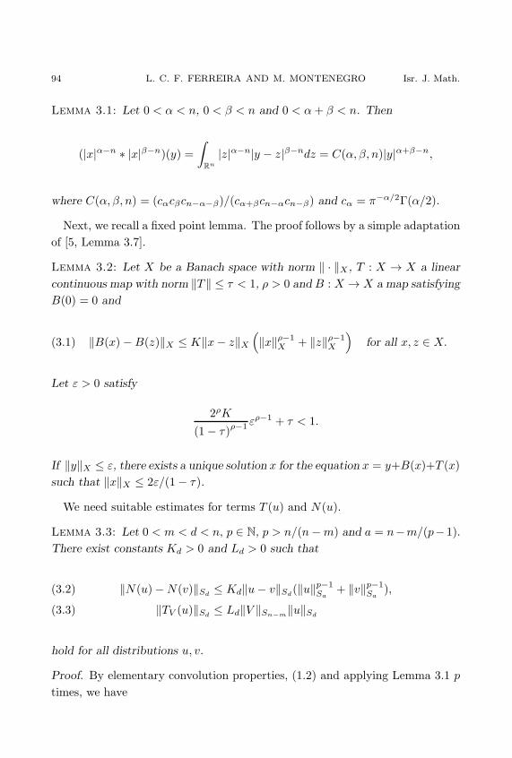
Lemma 3.1: Let 0 < α < n, 0 < β < n and 0 < α+ β < n. Then
(|x|α−n ∗ |x|β−n)(y) =
∫
Rn
|z|α−n|y − z|β−ndz = C(α, β, n)|y|α+β−n,
where C(α, β, n) = (cαcβcn−α−β)/(cα+βcn−αcn−β) and cα = π−α/2Γ(α/2).
Next, we recall a fixed point lemma. The proof follows by a simple adaptation
of [5, Lemma 3.7].
Lemma 3.2: Let X be a Banach space with norm ‖ · ‖X , T : X → X a linear
continuous map with norm ‖T ‖ ≤ τ < 1, ρ > 0 and B : X → X a map satisfying
B(0) = 0 and
(3.1) ‖B(x)−B(z)‖X ≤ K‖x− z‖X(
‖x‖ρ−1X + ‖z‖ρ−1
X
)
for all x, z ∈ X.
Let ε > 0 satisfy
2ρK
(1− τ)ρ−1 ε
ρ−1 + τ < 1.
If ‖y‖X ≤ ε, there exists a unique solution x for the equation x = y+B(x)+T (x)
such that ‖x‖X ≤ 2ε/(1− τ).
We need suitable estimates for terms T (u) and N(u).
Lemma 3.3: Let 0 < m < d < n, p ∈ N, p > n/(n−m) and a = n−m/(p− 1).
There exist constants Kd > 0 and Ld > 0 such that
‖N(u)−N(v)‖Sd≤ Kd‖u− v‖Sd
(‖u‖p−1Sa
+ ‖v‖p−1Sa
),(3.2)
‖TV (u)‖Sd≤ Ld‖V ‖Sn−m‖u‖Sd
(3.3)
hold for all distributions u, v.
Proof. By elementary convolution properties, (1.2) and applying Lemma 3.1 p
times, we have

Vol. 193, 2013 FOURIER APPROACH FOR NONLINEAR EQUATIONS 95
∣
∣N(u)− N(v)∣
∣ =1
|σ(ξ)|∣
∣
∣
∣
(u ∗ u ∗ · · · ∗ u)︸ ︷︷ ︸
p-times
− (v ∗ v ∗ · · · ∗ v)︸ ︷︷ ︸
p-times
∣
∣
∣
∣
=1
|σ(ξ)|[
(u− v) ∗ u ∗ · · · ∗ u+ v ∗ (u− v) ∗ · · · ∗ u
+ v ∗ v ∗ (u− v) ∗ · · · ∗ u+ v ∗ v ∗ · · · ∗ (u− v)]
(3.4)
≤ M|ξ|m
(
1
|ξ|d ∗ 1
|ξ|a ∗ · · · ∗ 1
|ξ|a)
×[
‖u− v‖Sd‖u‖p−1
Sa+ ‖u− v‖Sd
‖v‖Sa‖u‖p−2Sa
+‖u− v‖Sd‖v‖2Sa
‖u‖p−3Sa
+ · · ·+ ‖u− v‖Sd‖v‖p−1
Sa
]
≤ C
|ξ|m(
1
|ξ|n−(n−d)∗ 1
|ξ|n−(n−a)∗ · · · ∗ 1
|ξ|n−(n−a)
)
× ‖u− v‖Sd
[
‖u‖p−1Sa
+ ‖v‖p−1Sa
]
=C
|ξ|m(cn−a)
p−1cn−m
cp−1a cm
cn−dcmcd−m
cn+m−dcdcn−m
×(
1
|ξ|n−(n−d)−(p−1)(n−a)
)
‖u− v‖Sd
[
‖u‖p−1Sa
+ ‖v‖p−1Sa
]
=Kd1
|ξ|d ‖u− v‖Sd
[
‖u‖p−1Sa
+ ‖v‖p−1Sa
]
,(3.5)
where we have used in (3.5) that (p − 1)(n − a) = m. Also, we can estimate
operator TV as
|TV (u)| ≤ C
|ξ|m |V | ∗ |u|
≤ 1
|ξ|m(
1
|ξ|n−m∗ 1
|ξ|d)
( supξ∈Rn
|ξ|n−m|V (ξ)|)( supξ∈Rn
|ξ|d|u(ξ)|)
=1
|ξ|m(
1
|ξ|n−m∗ 1
|ξ|n−(n−d)
)
‖V ‖Sn−m‖u‖Sd
=Ld1
|ξ|m(
1
|ξ|n−m−(n−d)
)
‖V ‖Sn−m‖u‖Sd=Ld
1
|ξ|d ‖V ‖Sn−m‖u‖Sd.
The next lemma supplies an estimate in L1-norm of the Fourier Transform
of operators T (u) and N(u).

96 L. C. F. FERREIRA AND M. MONTENEGRO Isr. J. Math.
Lemma 3.4: Let s ≥ 0, 0 < m < d < n, p ∈ N , p > m/(n − m) and
a = n − m/(p − 1). There exist positive constants K1,s, ˜Kd,s, L1,s, ˜Ld,s such
that
‖N(u)−N(v)‖1,s ≤K1,s‖u− v‖1,s(‖u‖p−11,s + ‖v‖p−1
1,s )
+ ˜Kd,s‖u− v‖Sd(‖u‖p−1
Sa+ ‖v‖p−1
Sa),(3.6)
‖TV (u)‖1,s ≤L1,s‖V ‖1,s‖u‖1,s + ˜Ld,s‖V ‖Sn−m‖u‖Sd(3.7)
hold for all distributions u, v.
Proof. Let us denote 〈ξ〉s = (1 + |ξ|s) and AR = {ξ ∈ Rn : |ξ| ≤ R}. We split
‖ 〈ξ〉s (N(u)− N(v))‖L1 =‖ 〈ξ〉s (N(u)− N(v))‖L1(AR)
+ ‖ 〈ξ〉s (N(u)− N(v))‖L1(ACR)
=I1 + I2.
Since d < n, by using (3.5) we estimate I1 as
I1 =
∫
AR
〈ξ〉s∣
∣
∣N(u)− N(v)∣
∣
∣ dξ
≤ Kd
∫
AR
(1 + |ξ|s)|ξ|d dξ‖u− v‖Sd
[
‖u‖p−1Sa
+ ‖v‖p−1Sa
]
= ˜Kd,s‖u− v‖Sd
[
‖u‖p−1Sa
+ ‖v‖p−1Sa
]
.(3.8)
Next we remind the reader of the inequality 〈ξ〉s ≤ C 〈ξ − z〉s 〈z〉s. For I2, we
use the last inequality, (1.2), (3.4) and apply the Young inequality in L1 to
obtain
I2 =
∫
ACR
〈ξ〉s∣
∣
∣N(u)− N(v)∣
∣
∣ dξ
≤ M|R|m
∥
∥
∥
∥
〈ξ〉s{
(u ∗ u ∗ · · · ∗ u)︸ ︷︷ ︸
p-times
−(v ∗ · ∗ v︸ ︷︷ ︸
p-times
)
}∥
∥
∥
∥
L1(Rn)
(3.9)
≤ M|R|m
[
‖u− v‖1,s‖u‖p−11,s + ‖u− v‖1,s‖v‖1,s‖u‖p−2
1,s
+‖u− v‖1,s‖v‖21,s‖u‖p−31,s + · · ·+ ‖u− v‖1,s‖v‖p−1
1,s
]
≤K1,s‖u− v‖1,s[
‖u‖p−11,s + ‖v‖p−1
1,s
]
.(3.10)

Vol. 193, 2013 FOURIER APPROACH FOR NONLINEAR EQUATIONS 97
Now (3.6) follows by adding (3.8) and (3.10). We leave the proof of (3.7) for
the reader, since it is similar to the proof of (3.6).
3.1. Proof of Theorem 1.1.
Proof of (i). We want to apply Lemma 3.2 to the integral equation (1.3) with
X = Sa, y = F (f), T (x) := TV (u) and B(x) := N(u).
Taking d = a in (3.2) and (3.3), we obtain the following estimates for N(u)
and TV (u):
(3.11) ‖N(u)−N(v)‖Sa ≤ Ka‖u− v‖Sa
(
‖u‖p−1Sa
+ ‖v‖p−1Sa
)
and
(3.12) ‖TV (u)− TV (v)‖Sa = ‖TV (u− v)‖Sa ≤ La‖V ‖Sn−m‖u− v‖Sa .
Clearly B(0) = N(0) = 0, and it satisfies the estimate (3.1) of Lemma 3.2
with X = Sa and K = Ka. From (3.12), observe that TV is a continuous linear
operator in X with norm ‖TV ‖ ≤ τa = La‖V ‖Sn−m < 1.
Also, we have
(3.13)
‖y‖X = ‖F (f)‖Sa = supξ∈Rn
|ξ|a|F (f)| ≤ supξ∈Rn
|ξ|a M|ξ|m | f(ξ)| = M‖f‖Sa−m .
Next, for 0 < ε < εa, notice that
(3.14)2pKa
(1− τa)p−1 ε
p−1 + τa < 1.
Assume that ‖f‖Sa−m ≤ ε/M. A direct application of Lemma 3.2 concludes the
proof of the existence assertion of (i). Finally, u = 1{|ξ|≤1}u+1{|ξ|>1}u ∈ L1+L2
since |u| ≤ C |ξ|−aand n/2 < a < n. Therefore u ∈ (L1+L2)∨ = L∞+L2.
Proof of (ii). Since we have applied Lemma 3.2, the solution u is the limit in
Sa of the following interaction:
(3.15) u1 = F (f) and uk+1 = F (f) +N(uk) + TV (uk) k ∈ N.
Next, we consider the sequence {wk}k≥2 given by wk+1 = uk+1−uk. Similarly
to the derivation of (3.13) we have
‖F (f)‖Sb= sup
ξ∈Rn
|ξ|b|F (f)| ≤ supξ∈Rn
|ξ|b M|ξ|m | f(ξ)| = M‖f‖Sb−m
.
98 L. C. F. FERREIRA AND M. MONTENEGRO Isr. J. Math.
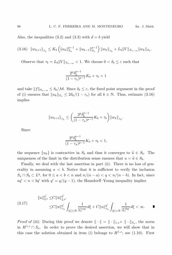
Also, the inequalities (3.2) and (3.3) with d = b yield
(3.16) ‖wk+1‖Sb≤ Kb
(
‖uk‖p−1Sa
+ ‖uk−1‖p−1Sa
)
‖wk‖Sb+ Lb‖V ‖Sn−m‖wk‖Sb
.
Observe that τb = Lb‖V ‖Sn−m < 1. We choose 0 < δb ≤ ε such that
2pδp−1b
(1− τa)p−1Kb + τb < 1
and take ‖f‖Sa−m ≤ δb/M. Since δb ≤ ε, the fixed point argument in the proof
of (i) ensures that ‖uk‖Sa ≤ 2δb/(1− τa) for all k ∈ N. Thus, estimate (3.16)
implies
‖wk+1‖Sb≤(
2pδp−1b
(1− τa)p−1Kb + τb
)
‖wk‖Sb.
Since
2pδp−1b
(1− τa)p−1Kb + τb < 1,
the sequence {uk} is contractive in Sb and thus it converges to u ∈ Sb. The
uniqueness of the limit in the distribution sense ensures that u = u ∈ Sb.
Finally, we deal with the last assertion in part (ii). There is no loss of gen-
erality in assuming a < b. Notice that it is sufficient to verify the inclusion
Sa ∩ Sb ⊂ Lq, for 0 ≤ a < b < n and n/(n− a) < q < n/(n− b). In fact, since
aq′ < n < bq′ with q′ = q/(q − 1), the Hausdorff–Young inequality implies
(3.17)
‖u‖q′Lq ≤C‖u‖q′Lq′
≤C‖u‖q′Sa
∫
|ξ|≤R
1
|ξ|aq′ dξ + C‖u‖q′Sb
∫
|ξ|>R
1
|ξ|bq′ dξ <∞.
Proof of (iii). During this proof we denote ‖ · ‖ = ‖ · ‖1,s+ ‖ · ‖Sa , the norm
in H1,s ∩ Sa. In order to prove the desired assertion, we will show that in
this case the solution obtained in item (i) belongs to H1,s; see (1.10). First

Vol. 193, 2013 FOURIER APPROACH FOR NONLINEAR EQUATIONS 99
we deal with the inhomogeneous term F (f). Taking R > 0, we split∫
Rn · · · =∫
|ξ|≤R · · ·+ ∫|ξ|>R · · · and estimate
(3.18)
‖F (f)‖1,s + ‖F (f)‖Sa
≤M‖f‖Sa−m
∫
|ξ|≤R
1
|ξ|a (1 + |ξ|s)dξ
+M∫
|ξ|>R
1
|ξ|m∣
∣
∣f∣
∣
∣ dξ +M‖f‖Sa−m
≤{
area(Sn−1)[p− 1
mpR
mpp−1 +
(p− 1
mp+ s)
Rmpp−1+s
]
+ 1}
M‖f‖Sa−m
+M|R|m
∫
|ξ|>R
∣
∣
∣f∣
∣
∣ dξ ≤ ε,
where we have used (3.13) and ε > 0 will be chosen later on.
Second, recalling that TV is a linear operator, we apply Lemma 3.4 with d = a
to obtain
(3.19)‖N(u)−N(v)‖1,s ≤K1,s‖u− v‖1,s(‖u‖p−1
1,s + ‖v‖p−11,s )
+ ˜Ka,s‖u− v‖Sa(‖u‖p−1Sa
+ ‖v‖p−1Sa
)
and
(3.20) ‖TV (u)− TV (u)‖1,s ≤ L1,s‖V ‖1,s‖u− v‖1,s + ˜La,s‖V ‖Sn−m‖u− v‖Sa .
Adding (3.11) to (3.19) and (3.12) to (3.20), we get
‖N(u)−N(v)‖ ≤ ˜K‖u− v‖(‖u‖p−1 + ‖v‖p−1),
‖TV (u)− TV (v)‖ ≤ τ‖u− v‖,
where ˜K=max{K1,s, ˜Ka,s+Ka} and τ=max{L1,s‖V ‖1,s, (˜La,s+La)‖V ‖Sn−m}<1.Next, take 0 < ε ≤ ε such that
2pεp−1
(1− τ )p−1˜K + τ < 1
and assume (3.18). Applying Lemma 3.2 in X = H1,s ∩ Sa, we obtain a
solution u ∈ H1,s ∩ Sa, which is the limit of the sequence (3.15) in norm
‖ · ‖ = ‖ · ‖1,s + ‖ · ‖Sa and, in particular, uk → u in Sa. By a fixed point
argument in the proof of (i), uk → u in Sa and then u = u and u ∈ H1,s ∩ Sa.
Since 〈ξ〉s u and 〈ξ〉s V ∈ L1, the Young inequality yields
〈ξ〉s |u ∗ · · · ∗ u| ≤ (| 〈ξ〉s u|) ∗ · · · ∗ (| 〈ξ〉s u|) ∈ L1

100 L. C. F. FERREIRA AND M. MONTENEGRO Isr. J. Math.
and
〈ξ〉s |V ∗ u| ≤ | 〈ξ〉s V | ∗ | 〈ξ〉s u| ∈ L1.
Denoting
h(ξ) = u ∗ · · · ∗ u+ V ∗ u+ f
and recalling AR = {ξ ∈ Rn : |ξ| ≤ R}, (1.3) implies
|∂αu| = |(−2πξi)αu| ≤ |2π||α| M|ξ|m−|α| |h(ξ)|
= 1AR
|2π||α|M|ξ|m−|α| |h(ξ)|+ 1AC
R
|2π||α|M|ξ|m−|α| |h(ξ)| .
By the Young inequality h(ξ) ∈ L1(Rn) because u, V , f ∈ L1(Rn). Since u ∈ Sa,
V ∈ Sn−m and f ∈ Sa−m, the proof of Lemma 3.3 tells us that h ∈ Sa−m. Thus
1AR
1
|ξ|m−|α| |h(ξ)| ≤ 1AR
1
|ξ|m−|α|‖h‖Sa−m
|ξ|a−m≤ C · 1AR
1
|ξ|a−|α| ∈ L1(Rn),
for all multi-index α, because a < n. Notice that 〈ξ〉s h(ξ) ∈ L1(Rn) and
1ACR
1
|ξ|m−|α| |h(ξ)| = 1ACR
1
|ξ|m−|α| 〈ξ〉s〈ξ〉s |h(ξ)|
≤ C1ACR|ξ||α|−m−s 〈ξ〉s |h(ξ)|∈L1(Rn) for all |α| ≤ m+s.
Thus ∂αu ∈ L1(Rn) and then ∂αu ∈ C0(Rn) when |α| ≤ m + s, that is,
u ∈ C[m+s]0 (Rn).
On the other hand, by elementary properties of the Fourier Transform and
since u, V ∈ L1(Rn), we have (u ∗ u ∗ · · · ∗ u)∨ = up and (V ∗ u)∨ = V u. Thus,
(3.21)
〈−L(u), ϕ〉 =〈−L(u), ϕ∨〉 = 〈−σ(ξ)u, ϕ∨〉=〈(u ∗ u ∗ · · · ∗ u), ϕ∨〉+ 〈V ∗ u, ϕ∨〉+ 〈f , ϕ∨〉=〈up, ϕ∨〉+ 〈(V u), ϕ∨〉+ 〈f , ϕ∨〉 = 〈up + V u+ f, ϕ〉,
for all ϕ ∈ S(Rn), and then u satisfies (1.1) in S ′(Rn). We conclude the proof
by observing that u is a classical solution because u, V, f,L(u) ∈ C0(Rn).
3.2. Proof of Theorem 1.2.
Proof of (i). If f is radial then so is f , and clearly u1 = F (f) because the
symbol σ(ξ) is radial. Since V is radial then TV (v) = V ∗ v is radial, provided
that v is radial. Also, B(v) is radial when v is radial. An induction argument
ensures that uk given by (3.15) is radial for all k ∈ N. Since uk → u in Sa,

Vol. 193, 2013 FOURIER APPROACH FOR NONLINEAR EQUATIONS 101
i.e., uk → u in supξ∈Rn |ξ|a| · |, and this norm preserves radial symmetry, then
u (and so u) is radial.
Now assume, by contradiction, that u is radial and let V be radial and f be
nonradial. Observe that if u and V are radial then F (f) = u− TV (u) −B(u)
and f = −σ(ξ)F (f) are radial, which contradicts the nonradial symmetry
of f .
Proof of (ii). We start by recalling that a distribution θ is homogeneous of de-
gree −(n−μ) if and only if θ is homogeneous of degree −μ. Since f is homoge-
neous of degree −mp/(p−1), one verifies that u1 given by (3.15) is homogeneous
of degree −a = −(n −m/(p − 1)). On the other hand, since V (ξ) is homoge-
neous of degree −(n −m), an induction argument and (1.3) prove that uk is
homogeneous of degree −a for all k ∈ N. Since the limit uk → u is taken with
respect to norm supξ∈Rn |ξ|a| · |, which is invariant by scaling (1.8), the solution
u must satisfy (by uniqueness of the limit)
u(ξ) = λau(λξ) a.e. ξ ∈ Rn, for all λ > 0,
showing that u is a homogeneous distribution of degree a − n = −m/(p − 1).
From Theorem 1.1 (i), u ∈ L∞ + L2 and thus u is a homogeneous function of
degree −m/(p− 1).
Proof of (iii). In order to show that u is a solution of (1.1), we will apply the
Inverse Fourier Transform in (1.3). For that matter, we need to prove that
(u ∗ · · · ∗ u)∨ = up and (V ∗ u)∨ = V u. In the proof of item (iii) of Theorem 1.1,
we used that u, V ∈ L1. This time, we cannot use this argument because ho-
mogeneous functions do not belong to L1(Rn). We will overcome this difficulty
by handling Lemma 3.1 in a suitable way. Assuming in addition that f, V are
radial, then u is radial and homogeneous of degree −m/(p− 1), so
(3.22) u(ξ) = γ11
|ξ|a , V (ξ) = γ21
|ξ|n−mand f(ξ) = γ3
1
|ξ|a−m,
where γi are constants. By Lemma 3.1
(3.23)
(u∗· · ·∗u)(ξ)=(
cn−a
ca
)pca−m
cn+m−a
γp1|ξ|a−m
and V ∗u =cn−acmca−m
cn+m−acacn−m
γ1γ2|ξ|a−m
,

102 L. C. F. FERREIRA AND M. MONTENEGRO Isr. J. Math.
where the constants cα are as in Lemma 3.1. Next, we recall an explicit formula
of the Fourier Transform of a homogeneous function, namely (cf. [15])
(3.24)
(
1
|ξ|d)∨
=cn−d
cd
1
|x|n−dfor all 0 < d < n.
By (3.23) and (3.24), since n− a = m/(p− 1), we have
u =
(
γ11
|ξ|a)∨
=cn−a
caγ1
1
|x|n−a=cn−a
caγ1
1
|x|m/(p−1)
and
(u ∗ · · · ∗ u)∨ =
((
cn−a
ca
)pca−m
cn+m−a
γp1|ξ|a−m
)∨
=cn−(a−m)
ca−m
(
cn−a
ca
)pca−m
cn+m−a
γp1|x|n+m−a
=
(
cn−a
ca
)pγp1
|x|mp/(p−1)= up.
An analogous computation yields (V ∗ u)∨ = V u. Therefore, using the last two
equalities and performing the same computation as in (3.21), one obtains that
u satisfies (1.1) in S ′(Rn). Finally, since u, V, f ∈ C∞(Rn−{0}) (by (3.22) and
(3.24)) we conclude that u satisfies (1.1) in a classical sense in Rn − {0}.
3.3. Proof of Theorem 1.3. First we derive an estimate about the behavior
at 0 and ∞ of the convolution operator with kernel |ξ|α−n which refines Lemma
3.1.
Lemma 3.5: Let 0 < α, β < n and C(α, β, n) be as in Lemma 3.1. If
supξ∈Rn
|ξ|n−β |g(ξ)| <∞,
then
lim sup|ξ|→0
|ξ|n−(α+β)∣
∣|ξ|α−n ∗ g∣∣ ≤ C(α, β, n) lim sup|ξ|→0
|ξ|n−β |g(ξ)|,(3.25)
lim sup|ξ|→∞
|ξ|n−(α+β)∣
∣|ξ|α−n ∗ g∣∣ ≤ C(α, β, n) lim sup|ξ|→∞
|ξ|n−β |g(ξ)|.(3.26)

Vol. 193, 2013 FOURIER APPROACH FOR NONLINEAR EQUATIONS 103
Proof. We will prove only (3.26). The proof of (3.25) is similar. Given R > 0,
for each fixed y �= 0, we have
sup|ξ|≥R
|(|ξ|y)|n−β |g(|ξ|y)| = sup||ξ|y|≥R|y|
|(|ξ|y)|n−β |g(|ξ|y)|
= sup|z|≥R|y|
|z|n−β|g(z)|.(3.27)
By using the change of variables y �→ |ξ|y we estimate
|ξ|n−(α+β)||ξ|α−n ∗ g|
≤ |ξ|n−(α+β)
∫
Rn
1
|ξ − y|n−α|g(y)|dy
=
∫
Rn
1∣
∣ξ|ξ|−1 − y∣
∣
n−α
1
|y|n−β|ξ|n−(α+β)+n−(n−α)|y|n−β|g(|ξ|y)|dy
=
∫
Rn
1∣
∣ξ|ξ|−1 − y∣
∣
n−α
1
|y|n−β|(|ξ|y)|n−β |g(|ξ|y)|dy.(3.28)
Taking the sup|ξ|≥R in (3.28) and using (3.27) we get
sup|ξ|≥R
|ξ|n−(α+β)∣
∣|ξ|α−n ∗ g∣∣
≤ sup|ξ|≥R
∫
Rn
1∣
∣ξ|ξ|−1 − y∣
∣
n−α
1
|y|n−β|(|ξ|y)|n−β |g(|ξ|y)|dy
≤ sup|ξ|≥R
∫
Rn
1∣
∣ξ|ξ|−1 − y∣
∣
n−α
1
|y|n−βsup|ξ|≥R
|(|ξ|y)|n−β |g(|ξ|y)|dy
≤ sup|ξ|≥R
∫
Rn
1∣
∣ξ|ξ|−1 − y∣
∣
n−α
1
|y|n−βsup
|z|≥R|y||z|n−β|g(z)|dy.(3.29)
Since
sup|ξ|≥R
1∣
∣ξ|ξ|−1 − y∣
∣
n−α =1
∣
∣1− |y|∣∣n−α
and∫
Rn
1∣
∣1− |y|∣∣n−α
1
|y|b dy = ∞,
in order to deal with (3.29) we shall not compute the sup within the integral in
(3.29). Our strategy is to split the integral into two parts,
sup|ξ|≥R
∫
Rn
G(ξ, y, R)dy ≤ sup|ξ|≥R
∫
|y|≥λ
G(ξ, y, R)dy + sup|ξ|≥R
∫
|y|<λ
G(ξ, y, R)dy
= I1(λ) + I2(λ),
104 L. C. F. FERREIRA AND M. MONTENEGRO Isr. J. Math.
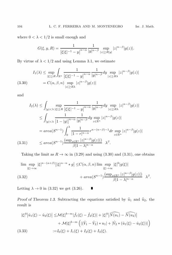
where 0 < λ < 1/2 is small enough and
G(ξ, y, R) =1
∣
∣ξ|ξ|−1 − y∣
∣
n−α
1
|y|n−βsup
|z|≥R|y||z|n−β|g(z)|.
By virtue of λ < 1/2 and using Lemma 3.1, we estimate
I1(λ) ≤ sup|ξ|≥R
∫
Rn
1∣
∣ξ|ξ|−1 − y∣
∣
n−α
1
|y|n−βdy sup
|z|≥Rλ
|z|n−β|g(z)|
= C(α, β, n) sup|z|≥Rλ
|z|n−β|g(z)|(3.30)
and
I2(λ) ≤∫
|y|<λ
sup|ξ|≥R
1∣
∣ξ|ξ|−1 − y∣
∣
n−α
1
|y|n−βdy sup
|z|≥Rλ
|z|n−β|g(z)|
≤∫
|y|<λ
1∣
∣1− |y|∣∣n−α
1
|y|n−βdy sup
z∈Rn
|z|n−β|g(z)|
= area(Sn−1)
∫ λ
0
1
|1− r|n−αrn−(n−β)−1dr sup
z∈Rn
|z|n−β|g(z)|
≤ area(Sn−1)(supz∈Rn |z|n−β|g(z)|)
β|1− λ|n−αλβ .(3.31)
Taking the limit as R → ∞ in (3.29) and using (3.30) and (3.31), one obtains
lim sup|ξ|→∞
|ξ|n−(α+β)∣
∣|ξ|α−n ∗ g∣∣ ≤C(α, β, n) lim sup|ξ|→∞
|ξ|b|g(ξ)|
+ area(Sn−1)(supz∈Rn |z|n−β|g(z)|)
β|1− λ|n−αλβ .(3.32)
Letting λ→ 0 in (3.32) we get (3.26).
Proof of Theorem 1.3. Subtracting the equations satisfied by u1 and u2, the
result is
|ξ|b∣∣u1(ξ)− u2(ξ)∣
∣ ≤M|ξ|b−m|f1(ξ)− f2(ξ)|+ |ξ|b∣∣N(u1)− N(u2)∣
∣
+M|ξ|b−m(
|(V1 − V2) ∗ u1|+ |V2 ∗ (u1(ξ)− u2(ξ))|)
:=I0(ξ) + I1(ξ) + I2(ξ) + I3(ξ).(3.33)

Vol. 193, 2013 FOURIER APPROACH FOR NONLINEAR EQUATIONS 105
We handle I1 as follows
(3.34)
|ξ|b∣
∣
∣N(u1)− N(u2)∣
∣
∣
≤|ξ|b M|ξ|m
∣
∣
∣
∣
[
(u1 ∗ · · · ∗ u1)︸ ︷︷ ︸
p−1
+(u2 ∗ · · · ∗ u1)︸ ︷︷ ︸
p−1
+ · · ·
+ (u2 ∗ u2 ∗ · · · ∗ u1)︸ ︷︷ ︸
p−1
+ · · ·+ (u2 ∗ u2 ∗ · · · ∗ u2)︸ ︷︷ ︸
p−1
]
∗ (u1 − u2)
∣
∣
∣
∣
≤M|ξ|b−m
[
(|ξ|−a ∗ · · · ∗ |ξ|−a)︸ ︷︷ ︸
p−1
∗|u1 − u2|]
×[
‖u‖p−1Sa
+ ‖v‖Sa‖u‖p−2Sa
+ ‖v‖2Sa‖u‖p−3
Sa+ · · ·+ ‖v‖p−1
Sa
]
≤C1|ξ|b−m
(
1
|ξ|n−(p−1)(n−a)∗ |u1 − u2|
)
[
‖u‖p−1Sa
+ ‖v‖p−1Sa
]
≤ 2pεp−1b C1
(1 − τa)p−1|ξ|b−m
(
1
|ξ|n−m∗ |u1 − u2|
)
.
Expressions I2 and I3 can be bounded directly in the following way:
|ξ|b−m∣
∣V2 ∗ (u1(ξ)− u2(ξ))∣
∣ ≤ ‖V2‖Sn−m |ξ|b−m(|ξ|m−n ∗ ∣∣u1 − u2
∣
∣
)
,(3.35)
|ξ|b−m∣
∣(V1 − V2) ∗ u1∣
∣ ≤ ‖u1‖Sb|ξ|b−m
(
|ξ|(n−b)−n ∗ ∣∣V1 − V2∣
∣
)
.(3.36)
The condition (1.14) implies lim sup|ξ|→∞ I0(ξ) = 0. Next, compute
lim sup|ξ|→∞ in (3.33)–(3.36) and afterwards apply (3.26) with α = m,β = n−band α = n− b, β = m to estimate
lim sup|ξ|→∞
|ξ|b|u1 − u2|
≤ lim sup|ξ|→∞
(I1 + I2 + I3)
≤(
2pδp−1b C1
(1− τa)p−1C(m,n− b, n) + ‖V2‖Sn−mC(n− b,m, n)
)
lim sup|ξ|→∞
|ξ|b|u1 − u2|
+ ‖u1‖Sblim sup|ξ|→∞
|ξ|n−m|V1 − V2|
=
(
2pδp−1b C1
(1− τa)p−1C(m,n− b, n) + ‖V2‖Sn−mC(n− b,m, n)
)
lim sup|ξ|→∞
|ξ|b|u1 − u2|.
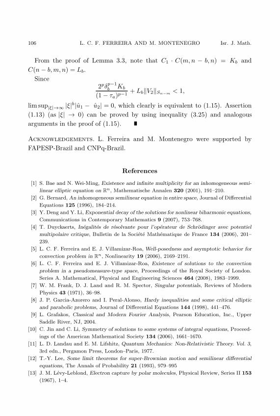
106 L. C. F. FERREIRA AND M. MONTENEGRO Isr. J. Math.
From the proof of Lemma 3.3, note that C1 · C(m,n − b, n) = Kb and
C(n− b,m, n) = Lb.
Since2pδp−1
b Kb
(1− τa)p−1+ Lb‖V2‖Sn−m < 1,
lim sup|ξ|→∞ |ξ|b|u1 − u2| = 0, which clearly is equivalent to (1.15). Assertion
(1.13) (as |ξ| → 0) can be proved by using inequality (3.25) and analogous
arguments in the proof of (1.15).
Acknowledgements. L. Ferreira and M. Montenegro were supported by
FAPESP-Brazil and CNPq-Brazil.
References
[1] S. Bae and N. Wei-Ming, Existence and infinite multiplicity for an inhomogeneous semi-
linear elliptic equation on Rn, Mathematische Annalen 320 (2001), 191–210.
[2] G. Bernard, An inhomogeneous semilinear equation in entire space, Journal of Differential
Equations 125 (1996), 184–214.
[3] Y. Deng and Y. Li, Exponential decay of the solutions for nonlinear biharmonic equations,
Communications in Contemporary Mathematics 9 (2007), 753–768.
[4] T. Duyckaerts, Inegalites de resolvante pour l’operateur de Schrodinger avec potentiel
multipolaire critique, Bulletin de la Societe Mathematique de France 134 (2006), 201–
239.
[5] L. C. F. Ferreira and E. J. Villamizar-Roa, Well-posedness and asymptotic behavior for
convection problem in Rn, Nonlinearity 19 (2006), 2169–2191.
[6] L. C. F. Ferreira and E. J. Villamizar-Roa, Existence of solutions to the convection
problem in a pseudomeasure-type space, Proceedings of the Royal Society of London.
Series A. Mathematical, Physical and Engineering Sciences 464 (2008), 1983–1999.
[7] W. M. Frank, D. J. Land and R. M. Spector, Singular potentials, Reviews of Modern
Physics 43 (1971), 36–98.
[8] J. P. Garcia-Azorero and I. Peral-Alonso, Hardy inequalities and some critical elliptic
and parabolic problems, Journal of Differential Equations 144 (1998), 441–476.
[9] L. Grafakos, Classical and Modern Fourier Analysis, Pearson Education, Inc., Upper
Saddle River, NJ, 2004.
[10] C. Jin and C. Li, Symmetry of solutions to some systems of integral equations, Proceed-
ings of the American Mathematical Society 134 (2006), 1661–1670.
[11] L. D. Landau and E. M. Lifshitz, Quantum Mechanics: Non-Relativistic Theory. Vol. 3,
3rd edn., Pergamon Press, London–Paris, 1977.
[12] T.-Y. Lee, Some limit theorems for super-Brownian motion and semilinear differential
equations, The Annals of Probability 21 (1993), 979–995
[13] J. M. Levy-Leblond, Electron capture by polar molecules, Physical Review, Series II 153
(1967), 1–4.

Vol. 193, 2013 FOURIER APPROACH FOR NONLINEAR EQUATIONS 107
[14] Q. Y. Li and Y. X. Ren, A large deviation for occupation time of super α-stable process,
Infinite Dimensional Analysis, Quantum Probability and Related Topics 11 (2008), 53–
71.
[15] E. Lieb and M. Loss, Analysis, 2nd edn., American Mathematical Society, Providence,
RI, 2001.
[16] F. Yang, Entire positive solutions for an inhomogeneous semilinear biharmonic equation,
Nonlinear Analysis. Theory, Methods & Applications 70 (2009), 1365–1376.
[17] H. Yin and P. Zhang, Bound states of nonlinear Schrodinger equations with potentials
tending to zero at infinity, Journal of Differential Equations 247 (2009), 618–647.