a framework for individual-based simulation of heterogeneous … · 2017-01-31 · c nezar...
TRANSCRIPT
A Framework for Individual-based Simulation ofHeterogeneous Cell Populations
by
Nezar Abdennur
A thesis submitted to theFaculty of Graduate and Postdoctoral Studies
in partial fulfilment of the requirements for the degree ofMaster of Science in Cellular and Molecular Medicine
with Specialization in Bioinformatics
Department of Cellular and Molecular MedicineFaculty of MedicineUniversity of Ottawa
c© Nezar Abdennur, Ottawa, Canada, 2012
Abstract
An object-oriented framework is presented for developing and simulating individual-based
models of cell populations. The framework supplies classes to define objects called simu-
lation channels that encapsulate the algorithms that make up a simulation model. These
may govern state-updating events at the individual level, perform global state changes,
or trigger cell division. Simulation engines control the scheduling and execution of col-
lections of simulation channels, while a simulation manager coordinates the engines ac-
cording to one of two scheduling protocols. When the ensemble of cells being simulated
reaches a specified maximum size, a procedure is introduced whereby random cells are
ejected from the simulation and replaced by newborn cells to keep the sample population
size constant but representative in composition. The framework permits recording of
population snapshot data and/or cell lineage histories. Use of the framework is demon-
strated through validation benchmarks and two case studies based on experiments from
the literature.
ii
Acknowledgements
I would like to thank my supervisor, Dr. Mads Kaern, for his guidance and support, as
well as my committee advisors, Dr. Theodore Perkins and Dr. Andre Longtin, for their
feedback.
I would also like to thank current members of the Kaern lab—specifically, Daniel
Charlebois, for helping to develop the replicative aging model and for proofreading the
thesis, and Hilary Phenix, for generously providing flow cytometry data. But mostly,
I would like to thank them both as well as lab members Alex Power, Daniel Jedrisiak
and Sarah Voll, for providing a stimulating work environment and simply for being great
colleagues and friends.
I am also grateful to Dr. Matthew Scott at the University of Waterloo for taking the
time to offer me a one-on-one crash course on stochastic processes just prior to beginning
my Master’s project. What I picked up in those few days laid the foundation for acquiring
knowledge on many of the topics that now permeate the pages of this thesis.
I would also like to thank a few “real” computer scientists—Georg Summer, Martina
Kutmon, and especially Andrei Anisenia—for valuable discussions which lead to great
improvements in the design of the framework.
Finally, I would like to thank my family and friends outside the academic environment
for their constant support and encouragement.
iii
Contents
1 Introduction 1
1.1 Heterogeneity in isogenic cell populations . . . . . . . . . . . . . . . . . . 1
1.2 Seeing heterogeneity . . . . . . . . . . . . . . . . . . . . . . . . . . . . . 2
1.3 Sources of heterogeneity . . . . . . . . . . . . . . . . . . . . . . . . . . . 4
1.3.1 Nonlinear dynamics . . . . . . . . . . . . . . . . . . . . . . . . . . 4
1.3.2 Stochasticity . . . . . . . . . . . . . . . . . . . . . . . . . . . . . 5
1.3.3 Division and inheritance . . . . . . . . . . . . . . . . . . . . . . . 7
1.3.4 Reproductive dynamics . . . . . . . . . . . . . . . . . . . . . . . . 8
1.4 Overview of the thesis . . . . . . . . . . . . . . . . . . . . . . . . . . . . 8
2 Background 10
2.1 Modeling individual cells . . . . . . . . . . . . . . . . . . . . . . . . . . . 11
2.1.1 Biochemical kinetics . . . . . . . . . . . . . . . . . . . . . . . . . 11
2.1.2 The stochastic simulation algorithm . . . . . . . . . . . . . . . . . 14
2.1.3 Division and cell physiology . . . . . . . . . . . . . . . . . . . . . 17
2.2 Modeling structured cell populations . . . . . . . . . . . . . . . . . . . . 19
2.2.1 Population balance equations . . . . . . . . . . . . . . . . . . . . 19
2.2.2 Individual-based models . . . . . . . . . . . . . . . . . . . . . . . 21
2.3 A framework for individual-based simulation . . . . . . . . . . . . . . . . 24
iv

3 The Framework 26
3.1 Simulation events as generalized reactions . . . . . . . . . . . . . . . . . 26
3.2 Object orientation and frameworks . . . . . . . . . . . . . . . . . . . . . 29
3.3 Design . . . . . . . . . . . . . . . . . . . . . . . . . . . . . . . . . . . . . 32
3.3.1 A simulation engine coordinates each individual . . . . . . . . . . 32
3.3.2 The simulation manager coordinates the engines . . . . . . . . . . 35
3.3.3 Execution patterns of simulation events . . . . . . . . . . . . . . . 36
3.4 Simulation meta-algorithm . . . . . . . . . . . . . . . . . . . . . . . . . . 40
3.4.1 Simulation engine . . . . . . . . . . . . . . . . . . . . . . . . . . . 40
3.4.2 Simulation manager . . . . . . . . . . . . . . . . . . . . . . . . . . 41
3.5 Implementation . . . . . . . . . . . . . . . . . . . . . . . . . . . . . . . . 50
4 Validation and Case Studies 54
4.1 Stochastic gene expression . . . . . . . . . . . . . . . . . . . . . . . . . . 54
4.1.1 Implementing an SSA simulation channel . . . . . . . . . . . . . . 55
4.1.2 Incorporating growth and division . . . . . . . . . . . . . . . . . . 58
4.1.3 Incorporating extrinsic sources of variability into the reaction kinetics 61
4.2 Differential reproduction and the constant-number method . . . . . . . . 66
4.2.1 Background . . . . . . . . . . . . . . . . . . . . . . . . . . . . . . 66
4.2.2 Model . . . . . . . . . . . . . . . . . . . . . . . . . . . . . . . . . 66
4.2.3 Results and discussion . . . . . . . . . . . . . . . . . . . . . . . . 69
4.3 Size and replicative lifespan in budding yeast . . . . . . . . . . . . . . . . 73
4.3.1 Background . . . . . . . . . . . . . . . . . . . . . . . . . . . . . . 73
4.3.2 Model . . . . . . . . . . . . . . . . . . . . . . . . . . . . . . . . . 75
4.3.3 Results and discussion . . . . . . . . . . . . . . . . . . . . . . . . 76
4.4 Epigenetic memory in the response to stress . . . . . . . . . . . . . . . . 78
4.4.1 Background . . . . . . . . . . . . . . . . . . . . . . . . . . . . . . 78
4.4.2 Model . . . . . . . . . . . . . . . . . . . . . . . . . . . . . . . . . 81
v

4.4.3 Results and discussion . . . . . . . . . . . . . . . . . . . . . . . . 85
5 Conclusion 90
References 96
A Simulator implementation 109
A.1 Classes . . . . . . . . . . . . . . . . . . . . . . . . . . . . . . . . . . . . . 109
A.2 Meta-algorithm implementations and performance . . . . . . . . . . . . . 111
B The birth-migration process 114
vi

List of Figures
1.1 Two experimental methods, flow cytometry and time-lapse microscopyprovide complementary perspectives of cellular dynamics. . . . . . . . . . 3
2.1 Time series of protein concentrations generated from deterministic andstochastic simulations of the same gene expression model. . . . . . . . . . 12
2.2 Population growth and balanced growth. . . . . . . . . . . . . . . . . . . 212.3 Cell chains, cell populations and the constant-number method. . . . . . . 23
3.1 Simulation event channels form the basic units of a simulation in the CPSframework. . . . . . . . . . . . . . . . . . . . . . . . . . . . . . . . . . . . 27
3.2 Pseudocode describing the methods of local and global simulation channels. 343.3 Relationship between simulation engines and the simulation manager. . . 363.4 The First-Engine Method meta-algorithm. . . . . . . . . . . . . . . . . . 443.5 The Asynchronous Method meta-algorithm. . . . . . . . . . . . . . . . . 483.6 Screenshot of a script that runs a simulation of a complete model. . . . . 523.7 Screenshot of a class definition file for a simulation channel that performs
cell division. . . . . . . . . . . . . . . . . . . . . . . . . . . . . . . . . . . 53
4.1 Validation of SSA simulation channel. . . . . . . . . . . . . . . . . . . . . 574.2 Joint density histograms of cellular volume and protein levels in the cases
of symmetric and asymmetric division. . . . . . . . . . . . . . . . . . . . 594.3 Lineage dynamics starting from a single cell in the cases of symmetric and
asymmetric division. . . . . . . . . . . . . . . . . . . . . . . . . . . . . . 604.4 Modified SSA algorithm for time-varying propensities. . . . . . . . . . . . 634.5 Simulating gene expression with extrinsic sources of fluctuation. . . . . . 654.6 Model of bistable phenotype switching and reproduction. . . . . . . . . . 674.7 Comparing the sizes of subpopulations in simulations with and without
the constant-number size cap. . . . . . . . . . . . . . . . . . . . . . . . . 694.8 Simulating the bistable switching model using the constant-number method. 704.9 Assessing the Nmax-dependence of the constant-number method. . . . . . 724.10 Theory of the size-limited replicative aging of budding yeast. . . . . . . . 744.11 Simulating size-dependent replicative aging in budding yeast. . . . . . . . 774.12 Gene expression noise and epigenetic memory. . . . . . . . . . . . . . . . 804.13 Experiments showing adaptive drift of URA3GFP-expressing yeast cell pop-
ulations under prolonged exposure to stress. . . . . . . . . . . . . . . . . 824.14 The Ornstein-Uhlenbeck process. . . . . . . . . . . . . . . . . . . . . . . 83
vii

4.15 Slower relaxation of fluctuations causes adaptive drift of the populationexpression distribution under stress and confers resistance. . . . . . . . . 86
4.16 Varying the position and steepness of the reproductive rate function. . . 884.17 Reversible adaptive drift of mean expression for different values of τ . . . 89
5.1 Possible extension of the framework. . . . . . . . . . . . . . . . . . . . . 93
A.1 UML diagram of main CPS framework classes in the MATLAB implemen-tation. . . . . . . . . . . . . . . . . . . . . . . . . . . . . . . . . . . . . . 110
viii

List of Tables
3.1 Types of simulation channels having different execution patterns . . . . . 38
ix

List of Algorithms
2.1 SSA (Direct Method) . . . . . . . . . . . . . . . . . . . . . . . . . . . . . 16
2.2 SSA (First-Reaction Method) . . . . . . . . . . . . . . . . . . . . . . . . 17
3.1 Simulation engine algorithm . . . . . . . . . . . . . . . . . . . . . . . . . 40
3.2 Gap closure procedure . . . . . . . . . . . . . . . . . . . . . . . . . . . . 41
3.3 The First-Engine Method . . . . . . . . . . . . . . . . . . . . . . . . . . 43
3.4 The Asynchronous Method . . . . . . . . . . . . . . . . . . . . . . . . . . 47
4.1 SSADirect simulation channel . . . . . . . . . . . . . . . . . . . . . . . . 56
4.2 RxnStep channel . . . . . . . . . . . . . . . . . . . . . . . . . . . . . . . 64
4.3 BarrierStep channel . . . . . . . . . . . . . . . . . . . . . . . . . . . . . 64
x

Chapter 1
Introduction
1.1 Heterogeneity in isogenic cell populations
Much of the study of cellular systems hinges on the implicit assumption that the in-
dividual cells of a population are similar or functionally identical, at least on average.
This is the basis for attaching meaning to macroscopic parameters like growth yield and
respiratory rate, or to the results of biochemical assays that measure average or aggre-
gate levels of analytes pooled from large numbers of cells [1]. However, such averaged or
macroscopic analyses can often be misleading. Take, for instance, the classic example of
the maturation of Xenopus frog oocytes, in which graded input of progesterone translates
into a graded population-averaged measurement of phosphorylation of p42 MAP kinase,
yet for individual cells, the maturation response is actually all-or-nothing [2]. In this case,
as in countless others, it is necessary to consider the heterogeneity of the population to
truly understand the underlying biological process.
Over the last few decades, a great deal of research has demonstrated that even ge-
netically identical cells in the same environment will exhibit substantial heterogeneity
in phenotype and physiology [3, 4, 5]. This applies not just to natural populations and
1

Chapter 1. Introduction 2
multicellular organisms, but even to clonal microbial cell cultures grown under axenic
laboratory conditions [6, 7]. This variability reflects the underlying dynamic character
of individual cells. It can have functionally important consequences, producing het-
erogeneous responses to perturbations such as drug treatments [8], or providing fitness
advantages in fluctuating or uncertain environments in the absence of significant genetic
variation [9, 10, 11].
1.2 Seeing heterogeneity
Advances in technology continue to offer ways of getting a closer look at the biological
dynamics of cells. Two technologies in particular, flow cytometry and time-lapse mi-
croscopy, have gained wide popularity and exemplify two different conceptual levels of
quantifying and analyzing cellular heterogeneity.
Flow cytometry is a high-throughput technique for the multiparametric analysis of the
physical and/or chemical characteristics of large numbers of cells in a population [6, 12].
It involves passing individual cells through an illumination zone in a hydrodynamically
focused stream of liquid and detecting optical scattering properties and/or the light
emission of one or more fluorescent labels simultaneously. These readings are sorted elec-
tronically into bins, forming histograms of the distributions of cell parameters. One thus
obtains physiological“snapshots” of the population composition at a given point in time
at single-cell resolution (see Figure 1.1A). One can further sort a heterogeneous mixture of
cells into two or more containers using a specialized method called fluorescence-activated
cell sorting (FACS), whereby the fluid stream is charged as it exits the fluidics system
and then passes through an electrostatic field to deflect cells to the appropriate container.
While flow cytometry measurements can be taken from a population at multiple time
points, the technique does not allow the same cell to be tracked over time.

Chapter 1. Introduction 3
A
Forward scatter
Sid
e sc
atte
r (1
)
800 850 900 950300
400
500
600
Forward scatter800 850 900 950
200
400
600
800
FP1 Log (GFP)
Cou
nt
100 102 104
250
500
gate
FP
1 va
lues
(G
FP
)
B
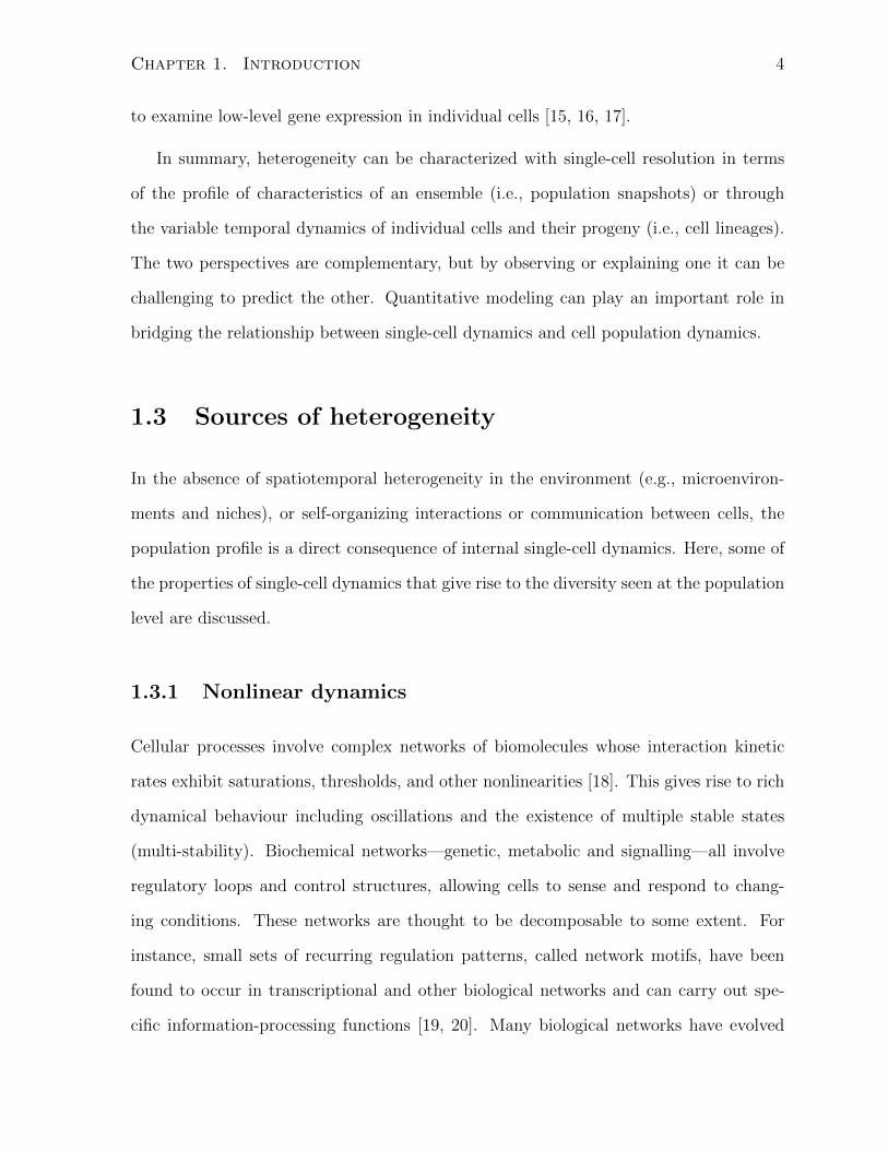
Figure 1.1: Two experimental methods, flow cytometry and time-lapse microscopy providecomplementary perspectives of cellular dynamics. (A) Flow cytometry enables multi-variateanalysis of single-cell light scattering properties and emission of fluorescent probes and stains.Shown are density plots and histograms from S. cerevisiae YPH499 cells expressing yeast-enhanced green fluorescent protein driven by the RNR3 promoter, whose transcriptional activityis responsive to a DNA-methylating drug. Data courtesy of H. Phenix. (B) Analysis of time-lapse microscopy images involves algorithms for segmentation of cells, feature quantification,and lineage tracking. Shown is the input and output from image analysis of a microcolony ofE. coli. Figure reproduced with permission from Locke et al. [13].
By contrast, time-lapse microscopy of live cells along with quantitative image analysis
allows the dynamics of individual cells and genealogical lineages to be followed over time
by photographing cells at regular time intervals over several hours (see Figure 1.1B). For
example, cells can be engineered to express fluorescent reporters for key genes, enabling
the characterization of the dynamics and physiological function of gene circuits as well
as correlations and the heritability of states, all at the single-cell level. Such movies have
provided many new insights into the behaviour of gene networks (for a review of recent
work, see [13]). In contrast to the throughput of flow cytometry, time-lapse microscopy
experiments are more time-consuming, large population statistics are harder to gener-
ate, and image analysis can be painstaking. However, advances in live-cell imaging and
microfluidics technologies are constantly improving the throughput and precision of live
cell microscopy experiments [14]. Furthermore, new molecular techniques are enabling
even closer inspection capabilities, such as the development of single-molecule detection
Chapter 1. Introduction 4
to examine low-level gene expression in individual cells [15, 16, 17].
In summary, heterogeneity can be characterized with single-cell resolution in terms
of the profile of characteristics of an ensemble (i.e., population snapshots) or through
the variable temporal dynamics of individual cells and their progeny (i.e., cell lineages).
The two perspectives are complementary, but by observing or explaining one it can be
challenging to predict the other. Quantitative modeling can play an important role in
bridging the relationship between single-cell dynamics and cell population dynamics.
1.3 Sources of heterogeneity
In the absence of spatiotemporal heterogeneity in the environment (e.g., microenviron-
ments and niches), or self-organizing interactions or communication between cells, the
population profile is a direct consequence of internal single-cell dynamics. Here, some of
the properties of single-cell dynamics that give rise to the diversity seen at the population
level are discussed.
1.3.1 Nonlinear dynamics
Cellular processes involve complex networks of biomolecules whose interaction kinetic
rates exhibit saturations, thresholds, and other nonlinearities [18]. This gives rise to rich
dynamical behaviour including oscillations and the existence of multiple stable states
(multi-stability). Biochemical networks—genetic, metabolic and signalling—all involve
regulatory loops and control structures, allowing cells to sense and respond to chang-
ing conditions. These networks are thought to be decomposable to some extent. For
instance, small sets of recurring regulation patterns, called network motifs, have been
found to occur in transcriptional and other biological networks and can carry out spe-
cific information-processing functions [19, 20]. Many biological networks have evolved

Chapter 1. Introduction 5
to be robust, in that they generate reliable output that is maintained in the face of
internal perturbations or external variations [21]. Today, synthetic biologists seeks to
both uncover and exploit the design principles of biological circuitry through the genetic
engineering of sensors, toggles, oscillators, pulse generators and more complex devices in
cells [22, 23, 24].
Importantly, the existence of multiple stable gene expression programs and robust
phenotypes conferred by biochemical networks gives rise to the type of differentiation
process described by C. H. Waddington (1957) in his metaphor of the “epigenetic land-
scape” [25], where cells spontaneously adopt stable phenotypes in a manner akin to
marbles rolling down hills towards “attracting” valleys. The shape of the landscape rep-
resents the phenotypic paths that cells can follow towards a stable cell type and the fate
of a cell is determined by the constant modulation of the epigenetic landscape by internal
and external signals. More recently, it has been suggested that this picture be extended
to consider the effects of molecular noise as a source of “thermal fluctuations” that move
cells around the landscape [26].
1.3.2 Stochasticity
The cellular milieu itself is a crowded, heterogeneous environment, with many macro-
molecular species present in very small copy numbers. This results in biochemical net-
works being subject to stochastic fluctuations or noise. Such effects have a critical role
in processes including cytoskeletal dynamics, cell polarization, and neural activity [27].
However, stochasticity has received the most attention, and is particularly acute, in the
case of gene expression [28].
It has become generally accepted that gene expression occurs in bursts, both of mRNA
and protein [15, 16, 17, 29]. Fluctuations in gene products are also propagated through
networks: they can be amplified or suppressed by regulation, or averaged away by slow

Chapter 1. Introduction 6
degradation of downstream elements [30, 31]. Gene expression noise is often described
in terms of intrinsic and extrinsic components. This is based on a landmark study
that quantified from image microscopy snapshots the variability or “noise”1 from two
identical copies of a promoter in E. coli driving the expression of different fluorescent
reporters [33]. The term intrinsic was used to refer to the variation that affected each copy
independently, while extrinsic referred to correlated variation in expression from the two
promoters. Generally, intrinsic fluctuations are those associated with noise generation,
while extrinsic fluctuations are attributed to noise propagation from other systems [30].
In the case of a single constitutive gene, the former would be due to bursting, while the
latter would be caused by variations in factors such as housekeeping machinery (e.g.,
levels of RNAP, ribosomes, ATP, ribonucleases and proteases), upstream regulators and
the cell cycle [5, 34].
Noise can be detrimental as it corrupts deterministic intra-cellular signals, but many
studies have shown that noise also provides critical functions and can facilitate evo-
lutionary adaptation and development. For example, stochasticity in gene expression
is implicated in several examples of cells assuming different and heritable fates in the
absence of genetic or environmental differences. Some documented examples of this
phenomenon, known as cellular decision making [26] or probabilistic differentiation [27],
include the decision of B. subtilis to initiate competence to take up DNA from the envi-
ronment under starvation [35, 36], the random activation of the galactose uptake system
in S. cerevisiae when exposed to a mixture of low glucose and high galactose [37], and
the random photoreceptor patterning of the ∼ 750 ommatidia of the compound eye of
D. melanogaster [38]. In all these cases, cell fate was found to be driven by noisy molec-
ular circuitry.
1This use of the term noise is to refer to a measure of population variation, usually the coefficientof variation (standard deviation divided by the mean) [32]. The interchangeable use of the term isunfortunate, because it can misleadingly give the impression that measured heterogeneity only reflectsspontaneous differences in the timing of biochemical reaction events.

Chapter 1. Introduction 7
1.3.3 Division and inheritance
Another source of variation in cell populations is the cell division cycle. Progression
through the cell cycle involves the modulation of many enzymes, transcriptional reg-
ulators, and signalling cascades, increased gene copy number due to DNA replication
and overall cell growth. A major contribution to population heterogeneity is that cells
are typically unsynchronized in culture, unless specifically manipulated to be [39]. The
same applies to other biological rhythms in the absence of mechanisms to entrain or
synchronize cells by some external signal or cell communication.
Cell division entails the redistribution of cell volume, membrane surface area, or-
ganelles, macromolecules, metabolites, and other components between newborn cells.
Asymmetry and noise in endowment can generate significant variation and often has
important biological consequences. While some components, like DNA, are segregated
evenly and in a highly ordered fashion, other organelles and macromolecules have been
observed to follow independent or at least mildly disordered partitioning, which gives
rise to some degree of stochastic partitioning error [40]. On the other hand, in many
species, some cellular contents are distributed asymmetrically between daughter cells.
Asymmetry in cell division can give rise to daughter cells with different fates. This can
occur, for example, in stem cell differentiation and self-renewal [41, 42]. Asymmetry is
also thought to be a key determinant of aging effects in some cell types. For example,
even though E. coli grows as a rod and divides in a morphologically symmetric manner,
fission produces one new cell pole per newborn per division event, resulting in age asym-
metry in a cell’s two poles. Stewart et al. [43] observed by time lapse microscopy that
cells which inherited older cell poles exhibited slower growth and increased incidence of
death.

Chapter 1. Introduction 8
1.3.4 Reproductive dynamics
One facet of population heterogeneity that is often underappreciated is heterogeneity in
proliferation. If a population consists of cells of different types or metabolic states which
possess different growth rates, then the population profile will be affected by the balance
between the rates of reproduction, quiescence and death of cells with different pheno-
types. For example, this is observed in the phenomenon of persistence in which bacteria
switch stochastically into a “persister” state, characterized by slower growth under nu-
trient abundance but increased immunity to environmental stresses, such as antibiotic
treatment [44]. The coexistence of the two subpopulations ensures survival of the popu-
lation in the face of unpredictable changes in the environment, while the environmental
conditions determine the relative sizes of the normal and persister subpopulations. Aging
is also typically associated with slower growth [43, 45], and the different growth rates
thus determine the age structure of the population.
1.4 Overview of the thesis
In a uniform environment that may be time-varying, the non-interactive sources of vari-
ability in an isogenic population of cells include the nonlinear and noisy dynamics of
biomolecular networks, asynchrony in oscillatory and non-steady processes, the statis-
tics and symmetry of endowment, and differential reproductive dynamics. Most cellular
modeling and simulation methodologies in systems biology do not incorporate all of these
sources, resorting either to detailed descriptions of idealized single cells (e.g., [34, 46]) or
coarse-grained descriptions of cell populations (e.g., [47, 48]). However, to truly bridge
the gap between the “snapshot” and “lineage” perspectives of cell heterogeneity requires
the ability to simulate the dynamics of structured cell populations based on models of
individual cells. The work here describes a computational framework to facilitate the
Chapter 1. Introduction 9
construction and execution of just such individual-based models. Chapter 2 provides the
background and motivation for the approach from a modeling perspective, while Chap-
ter 3 describes the object-oriented design of the simulation framework and a prototype
implementation in MATLAB. Chapter 4 demonstrates the use of the framework through
a set of validation benchmarks and two case study models. Finally, a general discussion
about the framework is provided in Chapter 5.

Chapter 2
Background
The sheer complexity of cellular processes puts limits on what can be gleaned from
qualitative reasoning based on static cartoons of molecular pathways, especially when
it comes to understanding cell-cell variability. As more molecular details come to light,
precise, quantitative descriptions—usually mathematical—are required to integrate the
information to describe the time-dependent biochemical or electrophysiological properties
of single cells or cell populations. Because rigorous mathematical analysis is usually only
possible for relatively simple models, computer simulation becomes an indispensable tool
for study as more complex dynamics are taken into account. Computational models
provide the means for the construction, analysis and testing of biological hypotheses in
silico, and for prediction and comparison with wet experiments. Section 2.1 describes
some common modeling approaches for single cells, which provides the motivation for
individual-based modeling of cell populations, discussed in Section 2.2.
10

Chapter 2. Background 11
2.1 Modeling individual cells
2.1.1 Biochemical kinetics
A goal of systems biology is to obtain predictive physicochemical models describing the
biochemical transformations that determine cellular physiology. The biochemical net-
works that shape the physiological properties of single cells are usually classified as gene
regulatory networks, signalling networks, and metabolic networks [49]. The most common
approach for modeling biochemical networks is the continuous, deterministic formalism
based on classical macroscopic chemical kinetics. The concentrations of each individual
biomolecular species in the system are modeled as continuous variables, whose tempo-
ral dynamics are driven by a system of ordinary differential equations (ODEs). The
terms of the ODEs represent rates of biochemical transformations including production,
consumption, complex assembly, and movement between compartments. Usually, ODEs
are formulated in terms of elementary reactions with mass action kinetics. However,
other algebraic rate laws such as Michaelis-Menten or Hill-type transfer functions are
often also used, either as phenomenological rate expressions, or as a simplification based
on timescale differences in the model (e.g., equilibrium or quasi-steady state assump-
tions) [50]. Other algebraic equations typically serve as constraints on the system.
Most ODE models of biochemical networks are complex and nonlinear and cannot
be solved analytically, so time trajectories are normally obtained by numerical solution
given a set of initial conditions. Model analysis is also largely computational in nature,
with several methodologies for sensitivity analysis (with close ties to engineering control
theory [51]), robustness analysis, and parameter estimation [52]. Biochemical network
models often involve many parameters to characterize the interactions between diverse
components. Parameter estimation, or model calibration, is a challenging task because
many rate parameters cannot be measured directly, but only constrained by experimental

Chapter 2. Background 12
0.15
0.10
0.05
0.000 4 8
Time (h)
Ab
und
ance
(µM
)
Probability
12 16 0.25 0.50
0.15
0.10
0.05
0.000 4 8
Time (h)
Ab
und
ance
(µM
)
Probability
12 16 0.1 0.2
a b
Figure 2.1: Time series of protein concentrations generated from deterministic and stochasticsimulations of the same gene expression model (blue and red curves, respectively) with his-tograms in the right-hand panels. (A) Low-amplitude fluctuations occur with high numbersof mRNA and protein molecules (∼ 3, 000 and 10, 000, respectively) and large cell volume(200µm3). (B) Fluctuations increase in amplitude with a decrease in the number of mRNAand protein molecules (to roughly 30 and 100, respectively) and smaller volume. Transcriptionrates were decreased and cell volume was decreased approximately 100-fold with compared with(A). Figure used with permission from Kaern et al. [28].
data and physical considerations [50, 52]. Because of the uncertainty in parameters and
difficulty in assessing small quantitative changes experimentally, an important approach
is to analyze the classes of qualitative behaviour a model can produce through bifurcation
analysis [53]. This can indicate, for instance, whether the steady states of a model are
stable or whether it can produce limit cycle oscillations.
The primary assumptions justifying use of the ODE formalism are that all com-
partments (e.g., cytoplasm, nucleus, etc.) remain well-mixed over the timescale of the
reactions being modeled, and that transport between compartments is slow enough to
be associated with an observable rate [50, 53]. If these assumptions are not satisfied,
then it is necessary to model changes in species concentrations explicitly with respect to
space (typically using partial differential equations). Another assumption is that species
concentrations can accurately be approximated as a continuum. When molecule numbers
are low, this is no longer valid and discrete stochastic fluctuations become significant [28]
(see Figure 2.1).

Chapter 2. Background 13
The stochastic formulation of chemical kinetics takes into account the fact that at the
molecular level, species levels change in discrete, integer amounts [54, 55]. Given a system
of molecules of N chemical species {S1, S2, . . . , SN} interacting via M chemical reactions
{R1, R2, . . . , RM}, the fundamental hypothesis of the stochastic formulation of chemical
kinetics supposes that there exists for each reaction Rj a stochastic reaction constant
cj such that cjdt is the average probability that a specific combination of Rj reactant
molecules will react in the next infinitesimal time interval dt. It is argued that this
assumption holds when the system is “well-mixed”, either through convective stirring, or
simply if non-reactive molecular collisions are much more frequent than reactive ones [54].
When the number of possibleRj reactant combinations hj is taken into account, we obtain
a quantity aj = hjcj called the propensity of reaction Rj such that
ajdt = the average probability that a Rj reaction will occur
in the system in the next infinitesimal time interval dt.(2.1)
Thus a reaction’s propensity is a function of the state of the system. To illustrate, if we
take the hypothetical dimerization reaction A + A → A2 with reaction constant c, and
denote the current number of A molecules in the system nA, then the number of distinct
A reactant molecule pairs that could combine would be nA(nA−1)/2. According to (2.1),
the current propensity of the reaction would then be c nA(nA − 1)/2.
Let Xi(t) denote the number of molecules of species Si in the system at time t and
νj denote the stoichiometric state-change vector associated with reaction Rj, specifying
how many molecules of each species is gained or lost by an Rj reaction event. The goal
is then to estimate the state vector X(t) := (X1(t), . . . , XN(t)), given that the system
is in state X(t0) = x0 at some initial time t0. The time evolution of the probability
P (x, t) := Pr{X(t) = x|X(t0) = x0} is governed by a differential-difference equation
called the chemical master equation (CME):

Chapter 2. Background 14
∂P (x, t)
∂t=
M∑j=1
[aj(x− νj)P (x− νj, t)− aj(x)P (x, t)] , (2.2)
which considers all transitions into and out of state x and can be derived from the
initial premise (2.1). The CME describes the probability distribution associated with
a continuous-time Markov process. 1 The CME is normally infinite-dimensional (it is
a set of coupled ODEs, with one equation for every possible combination of reactant
molecules); it can only be solved analytically in a few simple cases, and numerical solution
is often prohibitively difficult [56]. However, it turns out that single realizations of the
Markov process can easily be produced by numerical simulation, as described below. The
statistics of the probability density of X(t) can then be calculated from the results of
many realizations.
2.1.2 The stochastic simulation algorithm
Gillespie (1976 [54], 1977 [57]) first proposed the stochastic simulation algorithm (SSA)—
also known as the Gillespie algorithm—as a Monte Carlo procedure to generate realiza-
tions of the Markov process underlying the CME. Its formulation is based on the same
premise as the CME (2.1) and the algorithm is said to be exact in that it produces
trajectories that are in exact statistical agreement with the time-dependent probability
distribution governed by the CME. The development of the SSA is based on focusing
on a quantity called the Reaction Probability Density, P (τ, µ |x, t) which describes the
probability, given X(t) = x, that the very next reaction in the system will occur in the
infinitesimal time interval [t+ τ, t+ τ + dt) and will be an Rµ reaction. This was shown
to be
P (τ, µ|x, t) = aµ(x) exp
(−
M∑j=1
aj(x)τ
), (2.3)
1Also called a continuous-time Markov chain or jump Markov process.

Chapter 2. Background 15
which is related to the fact that the putative waiting time τi for an Ri reaction to
occur in the absence of other reaction channels is exponentially distributed according to
ai(x) exp (−ai(x)τi).
Gillespie presented two versions of the SSA, the Direct Method and the First-Reaction
Method, each of which samples distribution (2.3) in a different way to obtain values for
the time until the next reaction occurrence τ and which of the reactions it will be µ.
The system state is then updated by the stoichiometry of the reaction that fired and the
time is advanced by τ . This process is repeated until the simulation stop time is reached.
In the Direct Method (Alg. 2.1), two uniform random variates from the unit interval
are used to separately calculate τ and µ at each step. By contrast, the First-Reaction
Method (Alg. 2.2) uses M random variates to calculate each of the putative reaction
times τj, j = 1, . . . ,M . The reaction with the smallest reaction time, min(τ1, . . . , τM), is
then fired and all putative reaction times are recomputed. The First-Reaction Method is
usually less efficient than the Direct Method because it uses more random numbers and
because it wastefully resamples the putative reaction times from distributions that were
not affected by the last reaction event.
Gibson and Bruck [58] later developed an improved version of the First-Reaction
Method that makes clever use of data structures. Called the Next-Reaction Method, it
makes use of a dependency graph to denote the dependencies between reactions, thus
avoiding redundant reaction time recalculations. The search for the smallest reaction
time is also improved by scheduling reactions in absolute time (t+τj) rather than relative
time and storing them in a self-sorting data structure called an indexed priority queue.
Furthermore, the Next-Reaction Method is also able to “recycle” random variates so that
only a single one need be generated per time step.
Other optimized variants of the exact Direct and First-Reaction Methods have been
developed [59, 60, 61] as well as extensions to allow, for instance, the inclusion of delayed

Chapter 2. Background 16
Algorithm 2.1 SSA (Direct Method)
Require: System initialized at t = t0 with state x(t0) = x0
while termination condition is not satisfied do1. Evaluate and sum all propensities for the M reaction channels:
a0(x) =M∑j=1
aj(x).
2. Draw two unit-interval random numbers, r1 and r2.3. Calculate the time step to the next reaction event:
τ = − 1a0(x)
ln(r1).4. Determine identity of next reaction:
µ = the smallest integer satisfyingµ∑j=1
aj(x) > r2a0(x).
5. Update the system state x← x + νµ and time t← t+ τ .6. Record (x, t) as desired.
reactions [62] and spatial considerations [63, 64]. Because exact methods simulate each
reaction event explicitly, they become prohibitively slow as the total number of molecules
in the system increases. Several approximation methods have been developed to sacrifice
some accuracy for speed for large systems as well as for dynamically stiff systems. For
instance, the tau-leaping method, first introduced by Gillespie in 2001 [65] and elaborated
upon by numerous other [66], allows leaping in time steps τ that produce many different
reaction events, but only if τ satisfies a certain criterion known as the “leap condition”:
it must be small enough that no significant change occurs in any of the propensity values.
It can be shown that under conditions where the values of τ can be chosen so that each
reaction produces on average a very large number of firings, one can further approximate
the tau-leaping procedure by simulation of a continuous stochastic differential equation
known as a Langevin equation [56, 65]. Further taking the large-number limit where the
aj(x)τ →∞, the noise terms of the Langevin equation disappear, time evolution becomes
smooth, and one obtains deterministic reaction rate ODEs. Thus, the deterministic
formalism is recovered from stochastic chemical kinetics at the so-called thermodynamic

Chapter 2. Background 17
Algorithm 2.2 SSA (First-Reaction Method)
Require: System initialized at t = t0 with state x(t0) = x0
while termination condition is not satisfied do1. Evaluate the propensities for the M reaction channels: aj(x)2. Draw M random numbers r1, . . . , rM from the unit-interval and compute the
putative firing time steps:τj = − 1
aj(x)ln(rj).
3. Determine the time step to the next reaction event:τ = the smallest of the {τj}.
4. Determine the identity of the next reaction:µ = the index of the smallest of the {τj}.
5. Update the system state x← x + νµ and time t← t+ τ .6. Record (x, t) as desired.
limit (scaling up the species numbers and volume at a given concentration).
2.1.3 Division and cell physiology
Single-cell models tend to ignore or idealize the effects of cell growth and division. In
concentration-based ODE models, the dilution effect of cell growth is often lumped into
effective first-order degradation terms, but this is technically only correct if it can be
assumed that cell volume increases exponentially with time [67]. A similar trick is often
used in discrete stochastic models in which the effect of partitioning at cell division and/or
growth is approximated by having all components decay at a higher rate [68]. However,
growth and cell division can have important effects that cannot be averaged away, and,
in the worst case, their effects cannot be discriminated from those of intrinsic expression
noise. For example, it was demonstrated theoretically by Huh and Paulsson [40] that
fluctuations caused by segregation of gene products at cell division can propagate in a
way that mimic the effects of gene expression noise.
Chapter 2. Background 18
When the interest is in population dynamics and mechanisms of inheritance, division
and partitioning need to be handled explicitly. In the case of partitioning, when N
individual molecules or components are assumed to segregate independently, partitioning
can be simulated by drawing from a binomial distribution B(N, p). Models of more
disordered segregation (e.g., clustering due to packaging in vesicles) might be modeled
as a multinomial process [40]. Determining the timing of cell division and its connection
to other cellular processes varies with the scope of the model. In models that ignore size,
division could simply be treated as a periodic or random process. One option for using a
size-based threshold is the model of sloppy cell size control [69], which assumes individual
cells grow according to some specified growth law and, after reaching a minimum size,
divide with a probability that increases with increasing size.
On the other hand, simulations that explicitly account for cell division and inheritance
can be valuable for investigating the coordination of growth physiology, cell signalling,
size control and the cell cycle. Models may seek to explain how major transitions emerge
from molecular mechanisms. For example, mathematical models of the cell cycle in
yeasts yield DNA replication and nuclear division as an outcome of a dynamic signalling
network controlled by a relatively well-understood core regulatory machinery [70]. Con-
versely, the kinetics of gene expression are known to be intimately coupled to the growth
physiology of the cell. Even simple constitutive gene expression in exponentially growing
bacteria was shown to be strongly tied to global parameters such as basal transcriptional
and translational activity, gene dosage, and cell volume, all of which vary with growth
rate [71]. Some empirical growth laws for bacteria have recently been proposed that
integrate these observations but do not consider molecular details [72].

Chapter 2. Background 19
2.2 Modeling structured cell populations
2.2.1 Population balance equations
Population balance modelling is a name for a mathematical framework for describing
particulate systems such as aerosols, colloidal dispersions, and polymerization. The be-
haviour of a population of particles is described in terms of the behaviour of single
particles, taking into account birth and death processes (e.g., nucleation, fission, aggre-
gation), using a set of integro-partial differential equations known as population balance
equations (PBEs) [73]. These types of equations have been used to describe the time-
evolving structure of populations of proliferating cells by mathematical biologists and
bioprocess engineers since the middle of the twentieth century [74, 75].
Let F (x, t) represent the number or concentration of cells (number of cells per unit
volume), where x is a vector of extensive quantities representing the state of individual
cells. Typically, a single property, age or mass, is used as an index of cell state, but
other properties like chemical species and spatial coordinates could be included, giving
a higher dimensional state space. A population balance equation is a special case of
a general transport equation: an advection term takes into account the (deterministic)
flow of cells in the state space, a source term accounts for the creation of two newborn
cells, and a sink term accounts for the loss of mother cells that divide. In the simple one
dimensional case, say cell mass x, with no nutrient limitation and no cell death, the PBE
formulation of Fredrickson and co-workers [76] is as follows:
∂F (x, t)
∂t︸ ︷︷ ︸transient term
+∂
∂x[r(x)F (x, t)]︸ ︷︷ ︸
advection term
= − γ(x)F (x, t) + 2
∞∫x
p(x, x′)γ(x′)F (x′, t)dx′
︸ ︷︷ ︸source and sink terms
, (2.4)
where r(x) is called the growth rate function or velocity function of x, γ(x) is the division
rate function or fission intensity function that describes how the probability of a cell

Chapter 2. Background 20
dividing varies with x, and p(x, x′) is a partitioning function that describes the probability
of a parent cell that divides with mass x to produce two newborn cells with masses x′
and x−x′. A complete description thus requires formulations of r(x), γ(x), and p(x, x′),
boundary conditions, and an initial distribution F (x, 0).
A PBE is deterministic in that its time-evolution is uniquely determined by the initial
distribution. Theoretically, the PBE can be derived at the limit of very large population
size from a type of stochastic master equation describing the probability of the size and
composition of a finite and discrete population, in a way analogous to how deterministic
ODEs emerge from the chemical master equation at the thermodynamic limit [77]. In
the absence of nutrient limitation, the cell concentration normally grows exponentially
in time; however, the population distribution usually reaches a state where its shape
becomes time-invariant. In that case, the cell number density
f(t, x) =F (t, x)∫∞
0F (t, x)dx
(2.5)
reaches a steady state, with∫∞0f(t, x)dx = 1. This is usually referred to as the state
of “balanced growth” (see Figure 2.2) where all extensive properties of a cell culture
accumulate with the same specific growth rate [78]. PBEs can be formulated in terms of
the number density rather than the total number of cells [79].
PBE models are sometimes extended to include growth dependence on an external
substrate concentration S(t) [80]. One assumption in (2.4) is that all cells change state
according to the same deterministic law r(x). Incorporating more heterogeneity involves
adding more complexity to the model. For example, a diffusion term can be added to the
PBE to account for randomness in the evolution of the cells in state space (i.e., noise).
Furthermore, modeling discrete morphological stages or phases of the cell cycle requires
a set of coupled partial differential equations. Most PBEs cannot be solved analytically,
but can be discretized and integrated numerically. Unfortunately, with greater structure

Chapter 2. Background 21
0
10e6
0
0.5
1
0
balanced growthunbalanced growth
Num
ber
of c
ells
Num
ber
of c
ells
Rel
ativ
e nu
mbe
r of
cel
ls
A B10e6
F(x,t) F(x,t) f(x,t)
Figure 2.2: Population growth and balanced growth of an extensive property, such as cellmass. (A) Growth is unbalanced: Starting in one state (brown), the population changes in sizeand in composition to the grey histogram at a later time. (B) When growth is balanced thenumber of cells grows and the shape of the cell count histogram remains constant. Thus thehistogram normalized to the total number of cells becomes stationary. PBEs describe continuousfunctions, F (x, t) and f(x, t), that represent the “expectation” distributions corresponding tosuch histograms.
and higher dimensionality, not only do the functional terms and boundary conditions of a
PBE model become very complicated and difficult to formulate, but numerical integration
quickly becomes computationally intractable [80].
2.2.2 Individual-based models
A more direct approach to obtaining the composition of a population based on single-cell
descriptions is to simulate a sufficiently large ensemble of individual cells, which serve
as a finite, representative sample of the “true” population. This puts the entire toolkit
for single-cell simulation at our disposal without the difficulty of integrating complicated
and heterogeneous single-cell behaviour into a broader mathematical framework. While
most individual-based models are not amenable to mathematical analysis, their discrete
and computational nature places virtually no constraints on the types of heterogeneous
mechanisms that can be formulated and simulated.
In the case of simulating a population of non-dividing cells that do not interact locally,
the individual-based approach is usually as simple as performing numerous realizations of

Chapter 2. Background 22
a single-cell model. On the other hand, if cells can divide, then, starting with an initial
ensemble of cells, one might propose two possible approaches to obtain the long-term
population distribution:
1. Simulate the time courses of single cells, randomly choosing one of the two new-
borns to follow when a cell divides. The result is a collection of cell chains (see
Figure 2.3A).
2. Simulate the time courses of single cells, and continue to simulate all newborn cells
produced.
One problem with using the random cell chain approach for simulating cell population
dynamics is that it does not take into account the proliferative competition between cells
in different physiological states, and so will fail to provide the correct joint distribution of
cell properties except in the case where all of the cells divide at the same rate all the time.
Hence, the second approach must be used when dealing with a model in which the growth
rate of cells can vary with properties such as generational age, biochemical composition,
or cell type. Another drawback of the cell chain approach is that it cannot be used to
provide the temporal history of a complete genealogical cell lineage. However, the cell
chain approach can be valuable for investigating the range of phenotypes individual cells
can assume and how long they tend to reside in different states.
The problem with the second individual-based approach is that in simulations of
rapidly proliferating cells, the size of the simulation ensemble can rapidly grow to the
point of intractability. One way to get around this constraint is to use a Monte Carlo
technique called the constant-number method. This was originally developed as one of a
variety of so-called Monte Carlo methods to approximate the solution of population bal-
ance models of particulate processes through an individual-based approach rather than
through numerical integration of the continuous PBE model [81]. The idea is that the
number of particles being simulated is kept fixed but its composition still reflects the

Chapter 2. Background 23
time
cell chain
cell lineage
snapshot
+
cell division
random substitution
constant-number ensemble or "sample population"
A B
Figure 2.3: Cell chains, cell populations and the constant-number method.
number density of the true population. This is done by ejecting a randomly chosen indi-
vidual each time a new one is introduced, and copying a randomly chosen individual to fill
the vacancy produced when an individual is removed. By choosing the individual parti-
cles for substitution randomly, the statistical properties of the distribution remain intact.
Hence, through these resampling substitutions, the constant-number method maintains
statistical accuracy and can simulate growth over arbitrarily long times.
When simulating dividing cells, each time a cell divides, one can replace the parent cell
with one of the newborns, but a second surplus newborn cell is left over. In this context,
the constant-number method consists of substituting the surplus cell for one of the exist-
ing cells in the ensemble or “sample population”, where each cell has an equal probability
of being replaced, as depicted in Figure 2.3B. The constant-number method has recently
been applied to the simulation of heterogeneous populations. Specifically, Mantzaris used
the method in conjunction with deterministic [79] and stochastic Langevin [82] models
of single-cell dynamics, along with methods to determine the timing of cell divisions
and partitioning of cell contents that agree with the population balance formalism. The
constant-number method has also recently been incorporated into a parallel algorithm

Chapter 2. Background 24
for simulating stochastic gene expression using the Gillespie algorithm in growing and
dividing cells [83].
2.3 A framework for individual-based simulation
Ultimately, the scope and granularity of a model depends on the nature of the biological
problem being investigated. Based on what information is currently known about a sys-
tem, its complexity, and hypotheses being tested, judicious assumptions must be made
as to what processes can be ignored and to what degree one should inject into the model
detailed mechanisms vs. lumped descriptions and phenomenology. However as more com-
plexity is considered, it is not only the number of components but the multi-scale nature
of their interactions which makes both mathematical and computational analysis of bio-
logical systems challenging. For instance, as the need grows to integrate cell signalling,
metabolism, and gross physiology with division mechanisms and population dynamics,
hybrid simulation methods are required to handle the multiple temporal and spatial
scales involved [66]. Hybrid simulation implies the amalgamation of different algorithms,
and from a programming perspective seamless interaction between algorithms requires
the use of abstract programming interfaces and modular design. Object orientation is
one paradigm provides both the abstraction and extensibility to support the building of
these kinds of simulation models [84].
The work presented here is a general, object-oriented, computational framework for
developing and conducting individual-based simulations of cell populations. The frame-
work design is based on defining a set of software objects that serve as algorithmic prim-
itives of a simulation. There are primitives that drive the time evolution of the states
of individuals and others that execute global state changes. Correct scheduling and ex-
ecution of the primitives is coordinated by the framework meta-algorithm, allowing the
combination of simulation algorithms that execute continuous and discrete events with

Chapter 2. Background 25
different time-advancing mechanisms. The framework further supports single-cell, cell
chain and cell population dynamics simulations. In population dynamics simulations,
the framework regulates the production of newborn cells, allowing a simulation to begin
with as few as one cell and proceed until a pre-specified maximum population size is
reached, at which point resampling substitution (i.e., the constant-number method) is
introduced to keep a fixed sample population size with the appropriate composition. Fur-
thermore, the recording of either cell lineages, population snapshots, or other simulation
data, is easily implemented via the algorithmic primitives.

Chapter 3
The Framework
This chapter describes the design of a framework for simulating individual-based models
of cell populations called the cell population simulation (CPS) framework. Its purpose
is to provide a general means to manage the time evolution of the single cell models
and coordinate resampling substitution events and global events. Sections 3.1 and 3.2
provide the motivation behind the framework design, and sections 3.3 and 3.4 describe
the design and general algorithm. An implementation of the framework in MATLAB is
described in section 3.5.
3.1 Simulation events as generalized reactions
The conceptual basis for the simulation framework is essentially a generalization of the
notion of reaction channel in the stochastic simulation algorithm for chemical kinetics.
Recall that in a chemical reaction network, the system state is defined by a vector of
N species amounts x = (x1, x2, . . . , xN) in some state space S, which are modified by
a set of M reactions or reaction “channels”, labelled R1, R2, . . . , RM , where each Rj is
associated with a propensity function aj(x) : S → R and a state-change vector νj. When
an Rj reaction event occurs (or we can say, reaction channel Rj “fires”) after a time τ , it
26
Chapter 3. The Framework 27
Scheduling(variables read)
Execution(variables modified)Simulation channel
A,B X
X B,D
A
B
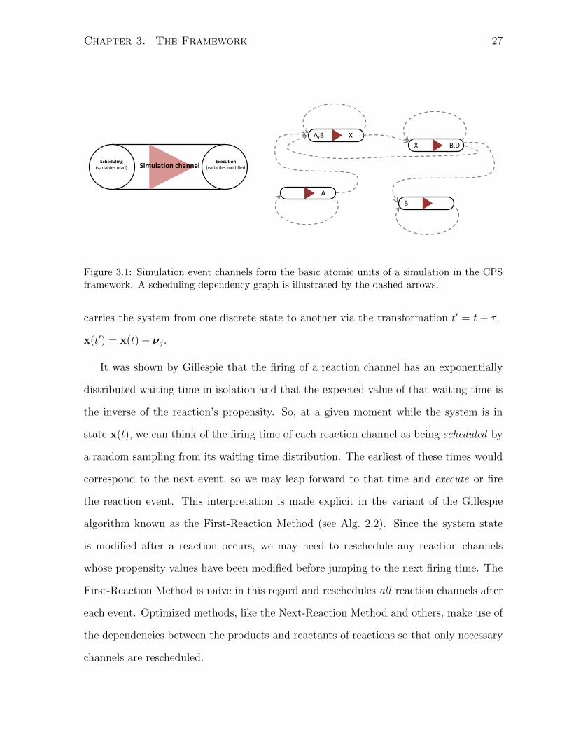
Figure 3.1: Simulation event channels form the basic atomic units of a simulation in the CPSframework. A scheduling dependency graph is illustrated by the dashed arrows.
carries the system from one discrete state to another via the transformation t′ = t + τ,
x(t′) = x(t) + νj.
It was shown by Gillespie that the firing of a reaction channel has an exponentially
distributed waiting time in isolation and that the expected value of that waiting time is
the inverse of the reaction’s propensity. So, at a given moment while the system is in
state x(t), we can think of the firing time of each reaction channel as being scheduled by
a random sampling from its waiting time distribution. The earliest of these times would
correspond to the next event, so we may leap forward to that time and execute or fire
the reaction event. This interpretation is made explicit in the variant of the Gillespie
algorithm known as the First-Reaction Method (see Alg. 2.2). Since the system state
is modified after a reaction occurs, we may need to reschedule any reaction channels
whose propensity values have been modified before jumping to the next firing time. The
First-Reaction Method is naive in this regard and reschedules all reaction channels after
each event. Optimized methods, like the Next-Reaction Method and others, make use of
the dependencies between the products and reactants of reactions so that only necessary
channels are rescheduled.

Chapter 3. The Framework 28
In general, we are interested in simulating not only the stochastic kinetics of small
numbers of reactant species, but arbitrary processes that may include cell growth, divi-
sion, metabolic fluxes, etc. and perhaps several processes occurring concomitantly. Ar-
bitrary dynamic processes affect one or more state variables of a cell—variables which
define the physiological state of the cell and may evolve deterministically or stochastically,
continuously or discretely. From a computational perspective, these processes translate
into simulation algorithms that perform a sequence of simulation events, and the goal is
to combine different algorithms with different stepping and updating rules, potentially
acting on the same data. The approach chosen here is to define simulation events in an
analogous way to the transition events of a reaction network Markov process.
As long as the putative time steps for state updates can be calculated from the sys-
tem state (i.e., simulation events can be scheduled) and the procedure for performing the
state updates can be specified (i.e., simulation events can be executed) in a well-defined
manner, then we can speak of generalized simulation event channels or simply, sim-
ulation channels. Simulation channels possess all the information required to schedule
and perform a particular simulation event when provided with the collection of state
variables defining the cell. They form the basic atomic units of a simulation in the
CPS framework. They perform two operations: scheduling, whereby the putative time
of a simulation event is determined; and execution, whereby the simulation event is per-
formed. When simulation channels are combined, they are related through a scheduling
dependency graph (see Figure 3.1). The dependency graph establishes the relationship
that a simulation channel that uses a variable for scheduling requires rescheduling when
another simulation channel modifies that variable. Simulation channels must also be
rescheduled after they execute an event.

Chapter 3. The Framework 29
3.2 Object orientation and frameworks
Using the notion of simulation channels, a model of phenotypic or physiological evolu-
tion of a cell would therefore consist of 1) defining of the state variables of a cell and 2)
defining the set of simulation channels that operate on the state variables. This would
serve as a flexible format for encoding models computationally. To conduct actual sim-
ulation runs, one can envision a simulation engine driving the simulation clock forward
and directing the scheduling and execution of the sequence of events through some type
of higher-level algorithm (here termed the simulation meta-algorithm) that uses the sim-
ulation channels supplied to it without the need to “know” the details of the model it is
simulating. Similarly, the definitions of the simulation channels do not have to depend
on the implementation details of the engine, so that the development and maintenance
of the two components is not strongly interdependent. Having a decoupled design is
valuable because it allows simulation channels to serve as pluggable, reusable modules
and confines their logic to the domain of the model they are being used to realize and
not to the underlying meta-algorithm used to execute them.
The type of system just described is well suited to an object-oriented approach. Today,
object-oriented programming (OOP) is a mainstream paradigm in software development,
but to the unfamiliarized, the terminology can be varied and confusing (especially since
everyday words are often used to denote specific programming features). Some of the
major concepts of OOP are briefly described in the following paragraphs. Obviously,
it does not do justice to the topic; it serves primarily to clarify the use of terms. For
more information, the unfamiliar reader may consult any popular textbook on OOP, such
as [85, 86].
OOP deals with data structures referred to as objects that possess both data and be-
haviour (i.e., operations that act on data). The data fields of an object are often referred
to as fields, member variables, properties or attributes while the procedures or operations
Chapter 3. The Framework 30
possessed by an object are usually called member functions or methods. Objects are the
actors of a program and interact by passing messages (i.e., calling methods). Constructs
called classes provide the blueprints to create objects of a particular type. Objects may
also be called class instances (object creation is also referred to as instantiation). While
in procedural programming, applications are designed primarily in terms of data flow
and data processing, in OOP design is focused on the conceptual entities that objects
represent and how they interact.
In OOP there is an important distinction between a class’s interface, normally consist-
ing of method declarations and describing what an object does, and the implementation
of those methods, which describes how the object does what it does. OOP supports
data encapsulation because classes provide well-defined public interfaces, consisting of
the fields and methods of an object accessible to its clients, while hiding and restricting
access to other members (e.g., private fields and methods are only accessible internally
by the object). Objects are usually assigned a responsibility, and classes are designed
around that responsibility and the data to be shared. Good object-oriented design should
focus on defining classes with a cohesive set of responsibilities and a low degree of mutual
interdependence. Encapsulation supports such a design.
In addition, classes can be extended through a feature called inheritance, whereby new
classes, known as derived classes or subclasses, inherit the attributes and behaviour of pre-
existing classes, known as base classes or superclasses. The inheritance relationship gives
rise to an inheritance hierarchy of types, which facilitates compartmentalization and code
reuse. Classes that provide one or more method interfaces without any implementation
can be defined; such abstract classes cannot be instantiated themselves, but through
inheritance different concrete classes with commonalities can be derived from an abstract
class. One use is to wrap different implementations of some input-output behaviour
beneath a common class interface to allow communication and integration with other
classes. Furthermore, subclasses can override the implementations of methods inherited

Chapter 3. The Framework 31
from a superclass, so that objects belonging to different classes respond to method calls of
the same name with different type-specific behaviour. This ability of subclass objects to
be used in place of objects resulting in different behaviour is referred to as polymorphism.
An important use of OOP is in the creation of software frameworks. These normally
refer to sets of libraries or classes that provide generic functionality which can be selec-
tively overridden or specialized by user code to provide specific functionality. While users
can extend a framework, they cannot modify its internal code. In this chapter, the con-
ceptual design of a simulation framework for simulating individual-based models of cells
is presented along with a working implementation of that design. The CPS framework
provides classes that serve as a standard interface for simulation event channels, which a
user may extend by defining his or her own channels that perform the simulation events
specific to a biological model. The internal framework components, however, handle the
simulation meta-algorithm. The former level of abstraction, dealing with the simulation
algorithms of a specific model, could be called the model layer, while the latter dealing
with the general meta-algorithm could be called the framework layer. OOP is a natu-
ral paradigm for such a layered design. In a similar vein, a naive end-user may not be
concerned with the details about how simulation events are performed algorithmically,
but he or she may want to simulate a fully formed model with specified set of model
parameters and initial conditions through an interface that hides the technical details
(such as a graphical user interface). This last “user interface layer” is concerned with
specific application development and is not dealt with in this work.

Chapter 3. The Framework 32
3.3 Design
3.3.1 A simulation engine coordinates each individual
The conceptual design of the CPS framework is described in this section. In the frame-
work, each cell is simulated as a separate individual. A simulation may also comprise
one or more global state variables that impact the entire collectivity or a subset of cells;
these variables are aggregated, giving rise to one additional “individual”. The most basic
types of objects used to perform a simulation at the individual level are described below.
Simulation entities are objects that encapsulate the state variables of an individual.
They expose their data to simulation event channels. The set of state variables that
an entity possesses are model-dependent. One entity class, Cell, represents individual
biological cells, and the state variables that cell entities encapsulate will be referred to
as local state variables. The other entity class, GlobalData, is used to encapsulate state
variables that may represent common environmental conditions or external resources
(e.g., temperature, drug concentrations), which will be called global state variables.
Simulation event channels, or simply, simulation channels, represent simulation
processes or algorithms that access and modify state variables, in analogy to the way
reaction channels modify species quantities in chemical network models. Simulation
channels can be of two subtypes, local or global, based on which type of entity they
are associated with. Simulation channel objects possess an attribute called eventTime,
which specifies the putative time of the next occurrence of a simulation event. Simulation
channel objects have two public methods: 1) schedule, which takes the current time and
a variable referencing the entity and as two of its input parameters and calculates the
value of eventTime, and 2) execute, which also takes a variable referencing the entity
as input and carries out a simulation event by performing some operation on the state
variables of the entity.

Chapter 3. The Framework 33
Because it is often the case that a local simulation channel requires information about
some global state variable in order to schedule a local simulation event, a reference
pointing to the global data entity is supplied to the schedule method as an additional
input parameter; however, access to the global variables should be read-only so as to
enforce the rule that simulation channels only modify their associated entity. Similarly,
an array referencing all of the cell entities individually (i.e., the ensemble) is supplied
to the schedule method of global simulation channels because the scheduling of global
simulation events may require querying the states of individual cells. Thus, the method
signatures of local and global simulation channel classes will resemble the pseudocode in
Figure 3.2.
The scheduling and execution of simulation events invoked upon each entity is man-
aged by a simulation engine that drives simulation forward. Each existing entity in
the simulation is paired with a unique simulation engine, which manages that entity’s
collection of simulation channels and its associated simulation clock. Because two types
of simulation entity were defined, we also define two subtypes of simulation engine. Keep-
ing the same naming pattern as for state variables and channels, those that handle cell
entities are called local simulation engines, while the single engine that handles the global
data entity is called the global simulation engine. Engines have the responsibility to keep
all simulation channels properly scheduled and to trigger the execution of the channel
corresponding to the earliest event time when instructed to do so. The simplest way to
keep the simulation channels properly scheduled would be to reschedule all simulation
channels after any given channel executes; however, that would be wasteful because gen-
erally not all simulation channels are affected by a given simulation event. Therefore,
a graph of channel scheduling dependencies is used by the engine so that the previous
channel that fired and those that depend on it are the only channels that get rescheduled
(see Figure 3.1).
A simulation engine thus possesses the entity, its associated simulation channels, the

Chapter 3. The Framework 34
class LocalSimulationChannel
public schedule(cell-entity†, global-data†, time). . .set the event time
public execute(cell-entity, global-data†, time, buffer). . .return boolean specifying whether cell-entity was modified
class GlobalSimulationChannel
public schedule(global-data†, Set〈cell-entity†〉, time). . .set the event time
public execute(global-data, Set〈cell-entity†〉, time). . .return boolean specifying whether global-data was modified
Figure 3.2: Pseudocode describing the methods of local and global simulation channels. Meth-ods receive as input the current time and references pointing to entity objects. A variablereferencing a buffer for storing newborn cells is passed to the execute method of local simula-tion channels. Objects that should not be modified within a method (this can be enforced insome languages) are labelled with †.
scheduling dependencies of the channels, and the clock as attributes. Other attributes
of the engine class include nextEventTime and nextChannel, which respectively spec-
ify when the next simulation channel will fire, and which of the channels it will be—
semantically, the equivalents of the parameters τ and µ of the Gillespie algorithm.
To simulate division (or, more correctly, cytokinesis), a cell entity object possesses a
method to allow a copy of itself to be made, which may be invoked within the execute
method of a simulation channel. The state variables of the two resulting cell entities may
then be modified or adjusted to simulate the partitioning of cellular contents resulting in

Chapter 3. The Framework 35
two newborn daughter cells. On return of execute, the first newborn cell is just the same
entity as the parent cell and takes its place, remaining actively associated with the engine
(i.e., the active cell entity). The second newborn cell entity is set aside temporarily by
placing it in a buffer; the buffer is held by the engine, which records the time of birth.
3.3.2 The simulation manager coordinates the engines
To some extent, each entity can be simulated independently of the others. However, the
complications that arise are 1) the division of cells, which results in the creation of a
new cell entity and potentially the random substitution of an existing cell entity with
the newly created one; and 2) the modification of global state variables, which may alter
the simulation of as many as all of the individual cells simultaneously. Therefore, a new
type of object is introduced whose job is to orchestrate the overall simulation. A single
simulation manager object is responsible for handling newly produced daughter cell
entities and for directing the execution of the individual simulation engines. When some
termination condition is satisfied, the simulation manager ceases execution of the engines
and ends the simulation.
The relationship between the two types of simulation engine and the simulation man-
ager are depicted in Figure 3.3. The simulation manager is responsible for directing and
synchronizing the execution of the local simulation engines and the global simulation
engine. The manager also gathers any newborn cell entities set aside by the local engines
and handles them appropriately. If the maximum number of local engines has not been
reached, the manager assigns the newborns to new local simulation engines; otherwise,
the manager performs substitution on existing local engines. The manager is also re-
sponsible for providing local engines with a reference pointing to the global data entity
and providing the global engine with references pointing to the cell entities to be used for
scheduling as described in 3.3.1. Moreover, when a global simulation channel fires, the

Chapter 3. The Framework 36
newborns
channels
Global data
channels
Local Engine Global Engine
Global data Ensemble
Simulation Manager
clock
nextChannelnextEventTime
nextChannelnextEventTime
clock
Cell entity
Handles newborn cell entities
Ensures rescheduling of local engines after a global event
Provides data to engines
Coordinates action of engines
Figure 3.3: Relationship between simulation engines and the simulation manager.
global engine will notify the manager about whether any global state variables have been
modified. If that is the case, the manager will instruct the local engines to reschedule all
of their simulation channels 1.
3.3.3 Execution patterns of simulation events
It is important to note that the term “simulation event” used here does not always
correspond to a discrete event at the conceptual level of the model of a physical system.
Strictly speaking, a simulation event is an increment in the simulation clock potentially
coupled with a change of one or more state variables. The former kind of events will be
called “model events” so as to distinguish them from purely algorithmic simulation events.
1Alternatively, some form of map of the dependencies between global channels and local channels,or between global state variables and local channels, could be introduced to optimize this reschedulingprocedure. This has not been attempted.

Chapter 3. The Framework 37
In the simulation literature, the pattern with which simulation events are executed is
usually divided into two categories: time-driven and event-driven [87].
In event-driven algorithms, simulation events are driven by a stream of time-stamped
model events; the simulation jumps from the time of one state change to the next,
skipping the dead time in between because the physical process being modeled does
not affect the variables between those time points. Examples include the simulation
of queuing models, continuous time Markov chains (e.g., the Gillespie algorithm), and
other discrete event processes. In these cases, the exact time of the next state change can
be predicted in advance. By contrast, a time-driven or time-stepping execution pattern
involves advancing the simulation clock with predefined time increments. There are at
least two cases when this pattern is necessary. The first is when one is simulating a
continuously changing variable by numerical approximation, such as a variable governed
by a differential equation in which appropriate time steps are required for numerical
accuracy and stability. The other case is when the timing of a discrete physical event
cannot be predicted in advance, but it depends on some conditional expression (such as
a variable crossing a threshold value) in order for it to be “triggered”. In such scenarios,
execution must step in small enough increments to capture the model event accurately.
Time steps can be fixed or adaptive, and state information could be used to adjust
the pace. Therefore rather than discrete and exact updating, time-driven algorithms
approximate the continuous monitoring or continuous updating of state variables.
Simulation engines can support a combination of simulation channels that follow dif-
ferent execution patterns. The execution pattern of a simulation channel can be classified
according to the mode of action of the schedule and execute methods. In the case of
an event-driven simulation channel, the schedule method assesses the current state of
its input entity and schedules the putative next state change, while the execute method
carries out the state change. For a time-driven simulation channel, the schedule method
would set the event time to be the current time t plus a time increment ∆t, while the

Chapter 3. The Framework 38
Table 3.1: Types of simulation channels having different execution patterns
Type of process Execution pattern State changediscrete-event event-driven alwayscontinuous time-driven alwaystriggered time-driven conditionalnull either never
execute method may or may not carry out a state change depending on whether the
model event has been triggered. If not, this is signalled to the simulation engine so that it
need not invoke any rescheduling dependencies (see Figure 3.2). Simulation channels can
further be categorized according to the type of physical process they are realizing and
whether or not state variables are always modified upon execution (see Table 3.1). The
examples of channels already described above are denoted as discrete-event, continuous
and triggered, respectively. Additionally, a simulation channel may be defined simply to
record data at certain points in time: such a “null” channel never causes a change in any
state variable.
A few subtle remarks regarding scheduling dependencies are appropriate. Firstly,
note that a simulation channel must always be rescheduled after executing—channels are
always self-dependent. However, a channel could also be rescheduled as a result of other
channels executing, and this would affect its scheduling pattern. For instance, suppose
that a simulation channel handling cell division has a schedule method that sets division
to occur immediately if the cell is deemed ready to divide, and further suppose that this
division channel is dependent on other simulation channels so that whenever they are
executed, the scheduling method of the division channel subsequently gets invoked. Then
the result is that the scheduling of the division channel is slaved to, or contingent on, the
execution pattern of the other channels. This, in turn, could make the actual execution
pattern of the division channel depend on what other kinds of channels it is associated
with. So, while the processes listed in Table 3.1 have well-defined execution patterns in

Chapter 3. The Framework 39
isolation, the execution pattern of a simulation channel may sometimes be determined
by context, that is, by the channels its scheduling depends on.
Secondly, it is often the case with hybrid simulation algorithms that the existence of
a relatively small time step creates an efficiency bottleneck [88]. Sometimes, fine-grained
time stepping is unavoidable due to large differences in the time scale of the physical
events being modeled by different channels. Other times, fine-grained time stepping of a
time-driven simulation channel can be used as a kind of trick that allows one to eliminate
the need for channel dependencies: if a channel triggers its own rescheduling frequently
enough, it does not need to be reminded every time some other channel modifies a state
variable by a small amount.
Applying a coarse-grained time step to a time-driven channel can improve efficiency,
but care must be taken when the simulation clock approaches a final time point or reaches
a time barrier where the simulation engine must stop. An event-driven channel does not
need to be executed once its next event time exceeds the time barrier because it is not
supposed to produce an effect during the intervening period leading up to the barrier. On
the other hand, a time-driven channel represents a continuous process. If a time-driven
simulation channel is scheduled to fire at a time beyond the barrier, then in order to
ensure that all state variables are properly updated, it ought to be made to fire exactly
at the time barrier before simulation terminates. Once again, if the channel’s time step
is sufficiently small, the error associated with the ignored time gap can be neglected.
Otherwise, a terminal simulation step needs to be enforced by the simulation engine.
Channels that require such a forced terminal step will be called gap channels.

Chapter 3. The Framework 40
3.4 Simulation meta-algorithm
3.4.1 Simulation engine
A simulation engine is equipped with a simulation entity and a collection of simulation
channels. Its clock is a measure of time elapsed in the model (i.e., model time, as opposed
to wallclock time or runtime). To instruct a simulation engine occupying a given point
in model time to conduct simulation over an interval of model time, it is provided with
a limit or time barrier at which to stop execution. The basic engine meta-algorithm
then follows a scheme analogous to the Next-Reaction or First-Reaction variants of the
Gillespie algorithm (Alg. 3.1).
If the user labels any of the simulation channels as being gap channels, then the
engine will perform a final step whereby the gap channels have their event times forcibly
set to the barrier time; they are then executed and the final rescheduling dependencies
are invoked (Alg. 3.2).
Algorithm 3.1 Simulation engine algorithm
Require: All simulation channels C1, C2, . . . , Cn of entity e are scheduled.
while clock does not exceed time barrier doFind simulation channel with earliest time stamp: Ci.Execute Ci event. Advance clock.Reschedule Ci.Reschedule dependent channels ⊆ {Cj | j 6= i}(select all if dependencies are not provided).

Chapter 3. The Framework 41
Algorithm 3.2 Gap closure procedure
if there are any gap channels thenfor each gap channel G do
if eventTime ≤ time barrier thenSet eventTime to time barrierExecute G event. Advance clock.Reschedule G and dependent channels.
3.4.2 Simulation manager
The individual simulation engines cannot run autonomously due to the occurrence of
global events and the substitution of cells; both entail some form of indirect “communi-
cation” between engines. Because of these restrictions, the entire collection of simulation
engines needs to advance jointly in model time to some extent. Here, two different
versions of the meta-algorithm for coordinating the execution of the simulation engines
are presented. Both have advantages and disadvantages but produce the same final re-
sult. Which one performs better ultimately depends on the nature of the model being
simulated and the data structures used to perform search operations.
The First-Engine Method
The simplest way for the simulation manager to coordinate the engines is to use the fact
that each engine “sees” the time of its next pending simulation event (the nextEventTime
attribute). The manager can simply take the earliest of these times and instruct the
corresponding simulation engine to execute the corresponding channel and invoke the
required scheduling dependencies. The result is that at each step the entire system is
synchronized in model time, with one minor exception. If any of the other engines possess
gap channels, then the engines are not truly synchronized until the time gaps are closed.
Fortunately, gap closure does not need to be performed at every step, but only just

Chapter 3. The Framework 42
before a global simulation event is executed. In addition, after a global simulation event
is executed, the simulation manager must instruct the local engines to reschedule their
channels. The pseudocode for the simulation meta-algorithm just described, called the
First-Engine Method, is given in Alg. 3.3.
The First-Engine Method is illustrated in Figure 3.4. Evidently, in the First-Engine
Method, global simulation events are the most costly since in every local simulation
engine they can trigger 1) the gap closure procedure prior to their execution and 2)
channel rescheduling following their execution.
The Asynchronous Method
In this section, an alternative meta-algorithm is presented that permits some degree of
concurrency or logical parallelism between the simulation engines. This would make it
possible to use parallel programming to improve the performance of simulation. However,
the meta-algorithm is valid regardless of whether the engines perform their computations
concurrently or in succession of one another. It is based on the parallel algorithm de-
scribed by Charlebois et al. [83].
Note that the simulation engines do not need to have their clocks synchronized in
model time at every step, as was the case in the first engine method. However, one can
see that if a local engine were permitted to execute a local simulation event with a time
stamp that surpassed that of a global simulation event before that same global event had
been executed, the causality rules of the model might be violated, thus producing invalid
results. The processing of events out of time stamp order is a frequent problem in parallel
and distributed simulation, and if it is allowed to happen, it can only be remedied by
devising methods that, whenever a conflict is detected, retract and reverse bad events
after they are executed or roll the system back to an earlier state [87].
To avoid dealing with such complications, we will attempt to stick to what is called a

Chapter 3. The Framework 43
Algorithm 3.3 The First-Engine Method
Require: Local simulation engines L1,L2, . . . ,LN , global simulation engine G
Initialization:1: Initialize entities2: for each simulation engine E do3: E: Schedule all simulation channels4: E: Find simulation channel with earliest time stamp
Main loop:5: while termination condition is not satisfied do6: Find the engine Enextwith the earliest nextEventTime7: if Enext∈ {L1,L2, . . . ,LN} then8: Enext: Execute the event associated with the corresponding nextChannel
9: Enext: Advance clock10: Enext: Reschedule nextChannel and dependent channels11: Enext: Perform gap closure procedure (Alg. 3.2)12: else if Enext== G then13: for each local engine L do14: L: Perform gap closure procedure (Alg. 3.2)
15: Enext: Execute the event associated with the corresponding nextChannel
16: Enext: Advance clock17: Enext: Reschedule nextChannel and dependent channels18: Enext: Perform gap closure procedure (Alg. 3.2)19: for each local engine L do20: L: Reschedule all simulation channels21: if any cell divided then22: Collect newborn cell entity, birth time, and copied channels23: if N < Nmax then24: Send to new local engine LN+1
25: LN+1: Schedule all simulation channels26: N ← N + 127: else28: Generate random index r ∈ {1, . . . , N}29: Perform substitution on local engine Lr30: Lr: Schedule all simulation channels
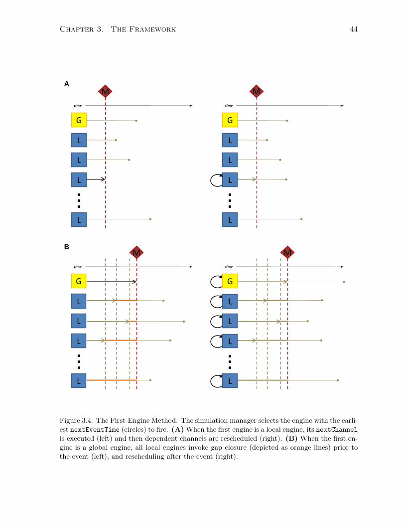
Chapter 3. The Framework 44
G
L
L
L
L
time
M
G
L
L
L
L
time
M
G
L
L
L
L
time
M
G
L
L
L
L
time
M
A
B
Figure 3.4: The First-Engine Method. The simulation manager selects the engine with the earli-est nextEventTime (circles) to fire. (A) When the first engine is a local engine, its nextChannelis executed (left) and then dependent channels are rescheduled (right). (B) When the first en-gine is a global engine, all local engines invoke gap closure (depicted as orange lines) prior tothe event (left), and rescheduling after the event (right).

Chapter 3. The Framework 45
conservative synchronization protocol [87], in which restrictions are put in place to prevent
the processing of events out of time stamp order. The goal, then, is for the simulation
manager to find the maximum “lookahead” for safe event execution and to use that time
as a synchronization barrier for the engines. The nextEventTime of the global simulation
engine serves as that barrier because none of the local simulation engines should surpass
that time point until the global simulation event is executed. Therefore, the simulation
manager establishes the synchronization barrier as the time of the next global event and
“releases” the local engines, which may proceed asynchronously until they reach it, racing
toward the finish line; once all have reached the barrier the global event can be executed.
However, a complication arises because cells may divide while the engines are en route
between barriers. The handling of division is not trivial because the simulation manager
performs resampling substitutions once the population reaches a size limit. There are
two cases:
1. Cell division is invoked by a global simulation channel.2
2. Cell division is invoked by a local simulation channel.
In Case 1, all newborn cells are produced when the population is already synchronized;
therefore, all of the substitutions occur in time stamp order. In Case 2, newborn cells
are produced in between synchronizations. This complicates things because the order
in which cells are created in wallclock time does not necessarily coincide with the time
stamp order of the model, but the random substitutions need to be performed in the
correct time stamp order.
Recall that when a cell entity divides, one of the resulting newborn cells takes the
place of the parent, while the other newborn cell is set aside, frozen at the time of
its birth. In order to handle Case 2, the solution is to proceed simulating the active
2Although, strictly speaking, this is prohibited in the current design as global channels are notsupposed to modify cell entities, the same effect can be achieved if a global channel notifies a localchannel to perform cell division through a change in a global state variable.

Chapter 3. The Framework 46
newborn cell entity until the synchronization barrier is reached. For generality, more
than one division is allowed to occur over the interval between barriers, and the extra
newborn cells produced are additionally stored. Once all the local engines reach the
synchronization barrier, a processing stage is reached. Here, the simulation manager
gathers all the pending newborn cell entities from the engines and sorts them by their
division time stamp so that they can be substituted back into the population (sent to
other local engines) in time stamp order (see Figure 3.5B). After that is done, because the
newly substituted cell entities were blocked at the time they were born, they too must be
advanced to the synchronization barrier by releasing their local engines. These cells may
also divide; hence, the procedure may be repeated if necessary until all the cell entities
are synchronized at the time barrier and no pending newborn entities remain. Then the
global event is executed and the next one is scheduled, providing a new synchronization
barrier. The pseudocode for the asynchronous method is listed in Alg. 3.4.
Case 1 is an option when cell division is event-driven, i.e., the exact time of cell
division can easily be calculated in advance (rarely the case). On the other hand, if
the division events for all cells were implemented using time-driven global simulation
channels, the granularity of the time stepping required to accurately capture all division
events would lead to very frequent synchronizations. If the goal is to exploit concurrency,
then one would want to reduce the number of synchronizations by implementing division
events using local simulation channels.
Unfortunately, Case 2 creates a different trade-off because it breaks the conservative
synchronization protocol. The first problem is that, at each barrier, whenever a newborn
cell entity replaces a random cell entity in the population, the destination engine’s clock is
wound back to the time of the new cell’s birth and the old cell is discarded, meaning that
the output of simulating the old cell from the substitution time to the barrier time is of no
consequence (see Figure 3.5B). This superfluous simulation effort would not occur using a
fully conservative algorithm like the first engine method. To minimize this performance

Chapter 3. The Framework 47
Algorithm 3.4 The Asynchronous Method
Require: Local simulation engines L1,L2. . . ,LN , global simulation engine G
Initialization:1: Initialize entities2: for each simulation engine E do3: E: Schedule all simulation channels4: E: Find simulation channel with earliest time stamp
Main loop5: while termination condition is not satisfied do
Set the next time barrier:6: tsync ← nextEventTime of G
Release the local engines:7: for each local engine L do8: L: Apply Alg. 3.1 and Alg. 3.2 with time barrier tsync
Process newborns:9: while there are any stored newborn cell entities do
10: Collect newborn entities c1,. . . ,cj, times of birth, indices of engines of origine1, . . . , ej, and copied channels.
11: Sort entities and engine indices by birth time stamp order (cσ1 ,cσ2 ,. . . ,cσj),(eσ1 ,eσ2 ,. . . ,eσj).
12: for i← 1 to j do13: if N < Nmax then14: Send newborn cσi to new local engine LN+1
15: N ← N + 116: else17: if Engine of origin Leσi has already received a newborn then18: cσi is surplus. Discard.19: else20: Generate random index r of destination engine.21: Perform substitution on Lr. Reset engine clock.
22: Release affected local engines to time barrier tsync
Synchronize:23: G: Execute next global simulation event24: G: Reschedule dependent global channels25: for each local engine L do26: L: Reschedule all simulation channels

Chapter 3. The Framework 48
M
L
L
L
L
division event: newborn
random substitution
time
G
L
L
L
time
M
L
superfluous simulation
surplus newborn
A B
Figure 3.5: The Asynchronous Method. (A) The simulation manager selects the next globalsimulation event as the synchronization barrier. The local engines then proceed independently(asynchronously) until reaching it. (B) Any newborns produced between synchronizations mustbe handled by the manager. Substitutions can result in superfluous simulation and surplusnewborns that get discarded.

Chapter 3. The Framework 49
penalty, the simulation manager would have to pace the synchronization frequency to
the rate of cell proliferation in the population, balancing the performance gain through
parallel execution with the performance loss due to superfluous simulation. Imposing
arbitrary synchronizations can be done by using global null simulation channels, which
perform no state modifications (see Section 3.3.3). Then the lengths of the inter-barrier
intervals of model time could be tuned manually by the user or adjusted adaptively
during the simulation run, for instance, by assessing cell reproduction rates through the
null channel’s schedule method. In practice, the periodic recording of data using a
global simulation channel often provides sufficient synchronizations.
The second problem with Case 2 is that it is possible for a newborn cell entity with a
certain birth-time stamp to be sent to a local engine whose cell entity divided at a later
time stamp. The newborn cell produced from this latter division event would never have
been produced by a fully conservative algorithm and needs to be discarded. Therefore,
during the newborn processing stage, such surplus newborns need to be detected and
filtered out before substitution (Figure 3.5B).
Parallelization
The principal motivation for the asynchronous method was to use parallel computing
to speed up single simulation runs. While the asynchronous method was developed
conceptually by treating engines as being fully concurrent, any actual implementation
of the asynchronous method is by no means restricted to this configuration. In one
case, each local simulation engine could each indeed behave as a separate computational
thread or process, all of which run simultaneously, or virtually so. Alternatively, the local
simulation engines could be distributed among a set of simultaneously running computer
processors, but on each processor they are “released” sequentially over each inter-barrier
interval of model time. In the limit of many processors (e.g., on a large grid), every

Chapter 3. The Framework 50
engine would be assigned to a single processor and we again obtain a fully concurrent
configuration. In the limit of a single processor, the result would be fully serial execution.
The meta-algorithm described in 3.4 is general because it does not specify how the local
engines should be “released”. The drawback of the asynchronous method is that it must
be carefully used to provide a performance benefit.
3.5 Implementation
An implementation of the CPS framework was developed in MATLAB, version 7.11
(R2010b). It implements both the First Engine Method (Alg. 3.3) and the Asynchronous
Method (Alg. 3.4) and uses the native Parallel Toolbox for parallelization. The Asyn-
chronous Method supports three different modes of execution, one in a fully sequential
manner which does not make use of the parallel toolbox, and two parallel modes which
make use of different language constructs from the toolbox. All versions of the meta-
algorithm were found to give consistent results. The main framework classes are stored
in a package called cps. The user extends the classes LocalChannel and GlobalChannel
to create custom simulation channels. Details about the implementation and a diagram
of the classes used are given in Appendix A.
A simulation run is performed directly by passing named input arguments to the main
simulation function, CpsSimulate. The inputs required to perform a simulation are: an
instance of each type of simulation channel to be used, along with the maximum number
of local engines (Nmax), the number of cell entities to start with (Ninit), strings specifying
the names of local and global state variables, and a handle to a user-defined initialization
function (InitFcn) that sets the initial values of all the state variables. The local and
global channel dependency graphs are provided as adjacency matrices (matrices of 0’s
and 1’s that specify the connectivity of nodes). If none are provided, a complete graph
is assumed. Screenshots of a script running a simulation and an example of a custom

Chapter 3. The Framework 51
simulation channel class definition are given in Figures 3.6 and 3.7.
The primary application of interest is to simulate isogenic cell populations, which
typically implies that each cell entity be governed by an identical collection of local sim-
ulation channels. Hence, the user need only provide a single collection of local simulation
channel objects which will be copied for each of the active cell entities. However, it would
not be difficult to extend the current implementation to handle simulations of cells that
have dissimilar collections of local simulation channels.
The main function requires that a global simulation channel of class Recorder (or
a class derived from it) be provided. A recorder simulation channel is used to record
snapshots of the synchronized system at specified sampling times. It uses another object
of a class called SimData to determine how to record data. This simulation data object
is returned by the main function when a run is completed. A simulation data object
possesses a method called snapshot that receives references pointing to the cell entities
and the global data from the recorder and is responsible for saving the state data of
interest. The simulation data object also stores simulation run information. Although
the snapshot method of the base class SimData performs no actual operation, two general
purpose simulation data classes are derived: one that stores all state variables in memory,
and one that saves all data to disk. If a user wishes to select exactly which variables
to record, this can be done by writing a custom subclass of SimData and overriding the
snapshot method. In order to record lineage data, one can use a local simulation channel
that copies data whenever a cell divides, as will be shown in Section 4.1.

Chapter 3. The Framework 52
function sd = example%--- Simulate a model of stochastic gene expression with growth and division ---
%Model parameters%-rate constantsp.kR = 0.8; p.kP = 0.05; p.gR = 0.1;p.gP = 0.002;%-stoichiometry matrixp.S = [ 1 0; -1 0; 0 1; 0 -1 ];%-growth ratep.kV = log(2)/1800; %30min doubling time
%Construct simulation channels%Each type of channel has a class definitiongch1 = cps.Recorder('RecordingTimes',[0 100 200 300 400 500], 'SimData', cps.SimDataToMem());lch1 = SSADirect('StoichMatrix', p.S, 'PropensityFcn', @propFcn);lch2 = Growth('tstep',30);lch3 = Division('binomProb',0.5);
%Dependency graph adjacency matrices (diagonal 0 elements are ignored)globDG = 1;locDG = [1 0 0; %ssa 0 1 0; %growth 1 1 1];%div
%Run simulation. (returns simulation data)sd = CpsSimulate('MaxNumCells', 2000,... 'InitNumCells', 10,... 'LocalChannels', {lch1,lch2,lch3},... 'LocalDG', locDG,... 'LocalGapChannelIdx', 2,... %growth is set as a gap channel 'GlobalChannels', {gch1},... 'GlobalDG', globDG,... 'LocalVars', {'X', 'V', 'Vthresh','tLast','root_id','node_id'},... 'GlobalVars', {'kR','kP','gR','gP','kV'},... 'InitFcn', @initFcn,... 'UserData', p,... %gets passed to initFcn 'Method', 'Async',... 'Mode', 'Serial'); end
function initFcn(cells, gdata, p)%set the initial global datagdata.State.kR = p.kR; gdata.State.kP = p.kP;gdata.State.gR = p.gR;gdata.State.gP = p.gP;gdata.State.kV = p.kV;
%set the initial states of the cellsfor i = 1:10 cells(i).State.X = zeros(1,2); cells(i).State.V = exp(rand*log(2)); cells(i).State.Vthresh = 2 + 0.05*randn; cells(i).State.tLast = zeros(1,1); cells(i).State.root_id = i; cells(i).State.node_id = 1;endend
Figure 3.6: Screenshot of a script that runs a simulation of a complete model.

Chapter 3. The Framework 53
classdef Division < cps.LocalChannel
properties %attributes defined by the Division classbinomProb
end
methods (Access = public)%Constructor function
% Set properties by passing property-value pairsif nargin > 0
for k = 1:2:length(varargin)
end end end
function%determine the time until volume threshold is crossed
%set the event timeself.setEventTime(time + tdiv);
end
function%cell division --- clone parent cellnew_cell = cell.copy();
%modify cell and new_cell to their post-division states xprev = cell.State.X;
xpart = binornd(xprev,self.binomProb); %binomial partitioningcell.State.X = xpart;
new_cell.State.X = xprev - xpart;%..., etc... %
%store new_cell in nbuffer
%signal that cell entities were modifiedtf = true;
endend
end %classdef
%Class defining a simulation channel that performs cell division
tf = execute(self, cell, gdata, time, nbuffer)
nbuffer.insert(new_cell);
schedule(self, cell, gdata, time)
tdiv = log(cell.State.Vthresh/cell.State.V)/gdata.State.kV;
channel = Division(varargin)
channel.(varargin{k}) = varargin{k+1};
%inherits getEventTime and setEventTime from base class cps.SimChannel
Figure 3.7: Screenshot of a class definition file for a simulation channel that performs celldivision.

Chapter 4
Validation and Case Studies
This chapter presents a set of simulation studies used to validate the implementation of
the CPS framework and demonstrate realistic use cases related to experimental studies
in the literature. In Section 4.1, algorithms are implemented to simulate stochastic
gene expression and to incorporate the effects of division and partitioning. Section 4.2
validates the built-in use of the constant-number method in a simple model of dynamic
subpopulations having different growth rates. Section 4.3 involves a model of aging and
senescence in budding yeast, while a model involving the interplay of environmental stress
and gene expression is presented in Section 4.4.
4.1 Stochastic gene expression
To validate the implementation of the CPS framework, a simulation channel was created
to conduct simulations of a well-characterized model of stochastic gene expression without
division. The results obtained are compared with previously derived analytical solutions.
Division and asymmetric endowment are then incorporated using additional channels
to demonstrate the framework’s ability to handle dynamics at the level of a single cell
lineage as well as at the level of the aggregate distribution of cellular properties. Finally,
54

Chapter 4. Validation and Case Studies 55
to demonstrate the versatility of the simulation channel formalism, an algorithm for
incorporating extrinsic variability into models of noisy gene expression was implemented
and tested.
4.1.1 Implementing an SSA simulation channel
First, we validate that the framework can reproduce the expected ensemble statistics of a
simple gene expression model in the absence of reproductive dynamics. The model chosen
is a “two-stage model” of expression of a single gene. It is a simplification of a three-stage
gene expression model that excludes the kinetics of promoter states. This can be justified
in the case of a constitutively expressed gene or the in case where the promoter kinetics
are fast relative to the rate of transcription so that they get averaged away [89, 90]. The
model assumes zero-order kinetics of transcription, first-order translation of mRNAs into
protein, and first-order degradation of the gene products. It is given by the following
elementary reactions:
∅ kR−→ R (4.1)
RkP−→ R + P (4.2)
RγR−→ ∅ (4.3)
PγP−→ ∅, (4.4)
where R is mRNA and P is protein. In 2002, Ozbudak et al. [91] used the two-state
model to explain the results of flow cytometry experiments using strains of B. subtilis in
which the transcriptional and translational rates of a fluorescent reporter gene were tuned
through modulation of an inducible promoter and targeted mutations to the ribosome-
binding site. In a more recent paper, Shahrezaei and Swain [92] derive closed analytical
solution to the master equation of the two-stage model. Under the assumption that

Chapter 4. Validation and Case Studies 56
γR/γP >> 1, which is realistic for most stable proteins, the steady state probability
distribution of protein level was shown to follow a negative binomial distribution
P (n) =Γ(a+ n)
Γ(n+ 1)Γ(a)
(b
1 + b
)n(1− b
1 + b
)a, (4.5)
where n is the number of protein molecules, a = kR/γP , b = kP/γR, and Γ is the Gamma
function.
One way to realize this model in the CPS framework would be to create a separate
simulation channel for each individual reaction channel, so that the framework naturally
reproduces a variation of the Next-Reaction version of the SSA. A different approach was
followed instead: a single simulation channel was created to implement the simulation of
the entire reaction network as a whole. The simulation channel implements the Direct
Method version of the SSA, and hence is named SSADirect. The class is designed to be
generic, so that by supplying it with a handle to a function that computes the required
propensities and with a matrix of reaction stoichiometries, it can simulate any reaction
network model. The responsibilities of the schedule and execute methods are divided
up as described in Alg. 4.1.
Algorithm 4.1 SSADirect simulation channel
. x is a state variable of the cell entity
. τ , µ, the propensity functions ai and the νj are properties of the channel
public Schedule(cell-entity, global-data, t)Compute propensities ai(x).Calculate τ and µ as in Alg. 2.1.eventTime ← t+ τ
public Execute(cell-entity, global-data, t, buffer)x← x + νµreturn True . cell-entity was modified
A global simulation channel was also used to record snapshots of data at specified
times. The pair of channels produced the results shown in Figure 4.1. Each simulation

Chapter 4. Validation and Case Studies 57
Figure 4.1: Validation of SSA simulation channel. (A,B) Steady-state distributions of proteinin the two-stage model with (A) kR = 0.1s−1, kP = 0.1s−1 and (B) kR = 0.01s−1, kP = 1s−1.In both cases, γR = 0.1s−1 and γP = 0.002s−1. (C) Mean expression and (D) coefficient ofvariation as a function of transcription rate for two values of translation rate.
used Ninit = Nmax = 5000 cells. The top panels show the steady state distribution
of protein with the same mean but obtained with different values of kR and kP . The
bottom panels map the relationship of mean protein expression 〈n〉 and the coefficient
of variation σn/〈n〉 with the transcription and translation rate parameters. They are
in excellent agreement with analytical results. Note that the distribution in 4.1B has a
significantly greater spread than that in 4.1A. The greater variance is due to expression
occurring in infrequent translational bursts. The ratio kP/γR, measures the average burst
size, that is, the average number of transcripts produced from a single mRNA molecule

Chapter 4. Validation and Case Studies 58
during its lifetime.
4.1.2 Incorporating growth and division
Next, cell division and the partitioning of gene product molecules is incorporated into the
model by introducing two new local simulation channels: one to update the cell volume
(Growth) and one to handle cell division (Division). Volume growth is assumed to be
uncoupled from the reaction kinetics. It follows a deterministic exponential law
V (t) = V0ekV t, (4.6)
where V0 is the initial volume and kV is the growth rate. The cell divides when it reaches
a threshold volume Vth. The threshold is sloppy, sampled from a normal distribution with
a mean value of Vth at each division. Upon division, the parental volume is apportioned
among the two newborn cells according to a fixed ratio f . The mRNA and protein
contents are distributed binomially with parameter p—this amounts to “flipping a coin”
for each molecule to determine to which cell it belongs. Two cases are considered: 1)
symmetric division, in which contents are split 1:1 (i.e., p = f = 0.5), and 2) asymmetric
division, in which contents are split 4:1 (i.e., p = f = 0.2). Because growth and reaction
kinetics are not coupled, only Division triggers the rescheduling of other channels. The
dependency graph looks like:
SSADirect Growth
Division
First, the two cases are simulated with Ninit = Nmax = 2, 000 using a global simulation
channel to record population snapshots. The cells are initialized at a random point in
the division cycle and with zero mRNA and protein. The joint density distributions of

Chapter 4. Validation and Case Studies 59
Figure 4.2: Joint density histograms of cellular volume and protein levels in the case of (A)symmetric division (1:1) and (B) asymmetric division (4:1). Asymmetry produces three dis-cernible density peaks.
protein content and volume at steady state are shown in Figure 4.2. Note that symmetric
division (4.2A) does not have a qualitative effect on the shape of the steady state pro-
tein distribution as compared to Figure 4.1, while strong asymmetry in division (4.2B)
produces a profile that is bimodal with respect to each of protein and volume.
Next, modified versions of the simulation channels described were used to produce the
full time courses of entire cell lineages instead of only population snapshot data. Instead
of holding single values, the state variables of the cells are made to be arrays that store
the time stamped event history of a cell during its life-cycle. To record lineage data,
just before a cell divides the modified Division channel saves the event history of the
cell to memory and resets the arrays for the daughter cells. The results of simulating
cell lineages starting with a single cell entity is shown in Figure 4.3, with the case of
symmetric division on the left and asymmetric division on the right.
Figure 4.3A/B and 4.3C/D show time traces of protein expression and cell volume,
respectively, of the individual cells superposed in grey. The time trace of a single random
cell chain is highlighted in each plot. The graphs displayed in 4.3E/F are lineage den-
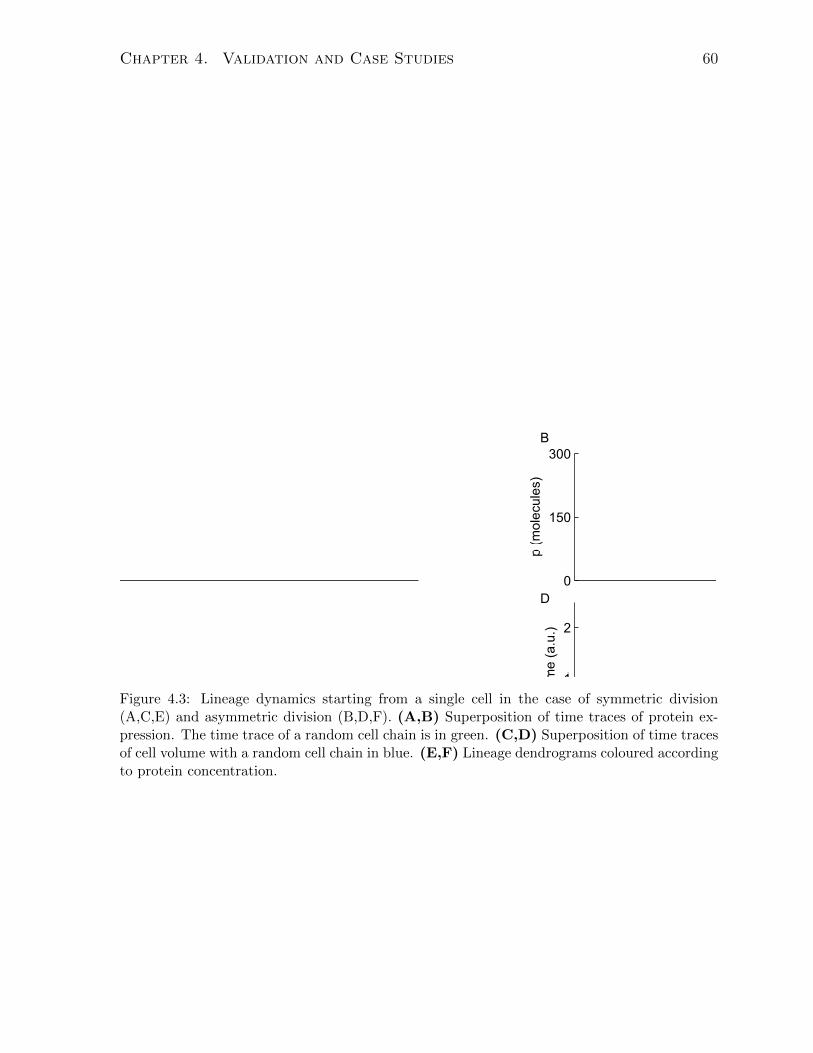
Chapter 4. Validation and Case Studies 60
Figure 4.3: Lineage dynamics starting from a single cell in the case of symmetric division(A,C,E) and asymmetric division (B,D,F). (A,B) Superposition of time traces of protein ex-pression. The time trace of a random cell chain is in green. (C,D) Superposition of time tracesof cell volume with a random cell chain in blue. (E,F) Lineage dendrograms coloured accordingto protein concentration.
Chapter 4. Validation and Case Studies 61
drograms that display the temporal and genealogical relationship between the cells. The
lines are coloured according to the protein concentration in order to provide a glimpse of
the internal dynamics of the individual cells over time.
The data shows a gradual desynchronization of the single-cell dynamics per generation
in the symmetric case due to noise in gene expression and sloppiness in the division cycle.
In the asymmetric case, division produces a large cell that divides sooner (reaches the
threshold volume rapidly) and a small daughter cell that divides much later, so that the
dendrogram is unbalanced. Note that in the case of symmetric division, both protein
number and volume drift continuously over the cell division cycle, while the protein
concentration does not change considerably. However, in the asymmetric case, early
after partitioning in the smaller daughter cells, protein levels rise proportionally more
rapidly than volume, producing a transient spike in concentration.
4.1.3 Incorporating extrinsic sources of variability into the re-
action kinetics
Much of the literature on stochastic gene expression has dealt with the problem of distin-
guishing noise origins from noise propagation in gene regulatory networks [27]. However,
stochastic models of gene networks usually consist of a simplified set of elementary re-
actions whose kinetic rates involve only the copy numbers of the components of the
network, that is, they only include sources of variability that are intrinsic to the system
being considered. They ignore sources of variability extrinsic to the components being
studied, such as variation of the elements of the transcriptional or translational machin-
ery of the cell, the changing cell volume, or the levels of upstream regulators. The overall
contribution of outside variables is thus tacitly “absorbed” into the rate constants of the
model reactions and assumed not to change. Part of the problem is that the exact sources
of extrinsic variability in gene networks are largely unknown and likely depend on the
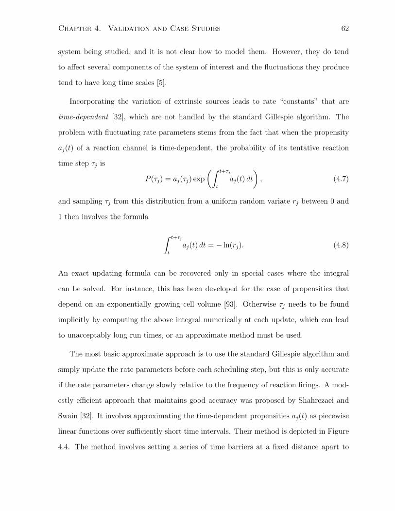
Chapter 4. Validation and Case Studies 62
system being studied, and it is not clear how to model them. However, they do tend
to affect several components of the system of interest and the fluctuations they produce
tend to have long time scales [5].
Incorporating the variation of extrinsic sources leads to rate “constants” that are
time-dependent [32], which are not handled by the standard Gillespie algorithm. The
problem with fluctuating rate parameters stems from the fact that when the propensity
aj(t) of a reaction channel is time-dependent, the probability of its tentative reaction
time step τj is
P (τj) = aj(τj) exp
(∫ t+τj
t
aj(t) dt
), (4.7)
and sampling τj from this distribution from a uniform random variate rj between 0 and
1 then involves the formula
∫ t+τj
t
aj(t) dt = − ln(rj). (4.8)
An exact updating formula can be recovered only in special cases where the integral
can be solved. For instance, this has been developed for the case of propensities that
depend on an exponentially growing cell volume [93]. Otherwise τj needs to be found
implicitly by computing the above integral numerically at each update, which can lead
to unacceptably long run times, or an approximate method must be used.
The most basic approximate approach is to use the standard Gillespie algorithm and
simply update the rate parameters before each scheduling step, but this is only accurate
if the rate parameters change slowly relative to the frequency of reaction firings. A mod-
estly efficient approach that maintains good accuracy was proposed by Shahrezaei and
Swain [32]. It involves approximating the time-dependent propensities aj(t) as piecewise
linear functions over sufficiently short time intervals. Their method is depicted in Figure
4.4. The method involves setting a series of time barriers at a fixed distance apart to

Chapter 4. Validation and Case Studies 63
tBt0
rate "constant" c(t)
propensity a(t)
A0
AB
-ln(r)
Figure 4.4: Modified SSA algorithm for time-varying propensities. Each time-dependentpropensity function is approximated by a piecewise linear function. See text for details.
serve as an upper bound on the size of the piecewise linear intervals. Assume the system
is at time t0 with state x(t0) and that the next barrier is at time tB. For simplicity,
assume only one reaction channel Rk is time-dependent with rate constant ck(t). Then
to calculate τk, the values of the rate constant at the two time points C0 = ck(t0) and
CB = ck(tb) are used along with the current state of the system x(t0) to calculate ak(t0)
(call it A0) and to estimate ak(tB) (call it AB). One can then approximate ak(t) locally
by the straight line joining A0 and AB. The area under the approximated ak(t) curve
is then a trapezoid and an explicit formula can be given to compute τk from a random
variate rk
τk =A0
α
(−1 +
√1− 2α
A20
ln(rk)
), where α =
AB − A0
tB − t0. (4.9)
If α = 0, then ak(t) is constant and the standard updating formula, τk = − ln(rk)/A0,
is used instead. The value of the next time step τ is then obtained as in the First-
Reaction method (Alg. 2.2). If t0 + τ < tB, the next reaction channel is fired. If instead
t0 + τ ≥ tB, the system is advanced to time tB, no reaction is fired, and the next barrier
is set at tB + T . The reactions are then rescheduled.
The procedure described in [32] was implemented in a novel way by using two sim-
ulation channels: one to handle the reaction firing steps RxnStep and one to handle
stepping to the time barrier BarrierStep (pseudocode in Alg. 4.2, 4.3). In terms of

Chapter 4. Validation and Case Studies 64
Algorithm 4.2 RxnStep channel
public Schedule(cell-entity, g-data, t)Calculate A0 and AB from C0 and CBCalculate τj ’sFind τ and µeventTime ← t+ τ
public Execute(cell-entity, g-data, t, b)C0 ← ck(eventTime)x← x+ νµreturn True
Algorithm 4.3 BarrierStep channel
public Schedule(cell-entity, g-data, t)eventTime ← tB
public Execute(cell-entity, g-data, t, b)C0 ← CBCB ← ck(tB + T )tB ← tB + Treturn True
scheduling dependencies, the execution of BarrierStep triggers scheduling of RxnStep,
but the reverse dependence is not required.
To test the implementation, we simulate extrinsic fluctuations in a three-stage gene
expression model, as in [32], where a continuous stochastic process drives the promoter
activation rate kON . To observe the effect of extrinsic noise, one usually measures the
output on two functionally identical “copies” of a system subject to the same extrinsic
fluctuations. This is shown in Figure 4.5, which plots the joint histogram of expression
data from two identical promoters collected at regular time points. The simulation on
the left involves only intrinsic noise; the joint distribution is spread quite evenly because
the sources of fluctuations are independent. On the right, a common source of extrinsic
fluctuations induce correlations which cause the distribution to become skewed along the
diagonal. The shapes of the distributions obtained agree with those in [32].

Chapter 4. Validation and Case Studies 65
extrinsic noise source
kON(t)
kOFF
kR kP
ɣR ɣP
kON(t)
kOFF
kR kP
ɣRɣP
Gene A
Gene B Gene B
Gene A
inactive promoter active promoter mRNA protein
A
B C
Figure 4.5: Simulating gene expression with extrinsic sources of fluctuation. (A) Three-stagegene expression model including promoter kinetics. A common extrinsic noise source drives thepromoter activation rates of the two reporter genes, kON (t) = k0ξ(t), where ξ(t) is a continuousstochastic process with a long autocorrelation time, as in [32]. (B,C) Joint distribution of twotime courses of gene expression in the (B) absence and (C) presence of a time-varying promoteractivation rate parameter kON (t).

Chapter 4. Validation and Case Studies 66
4.2 Differential reproduction and the constant-number
method
4.2.1 Background
It has been demonstrated that the CPS framework can handle combinations of state
updating algorithms along with cell division and partitioning, and can produce lineage
structures. In this section, it is demonstrated that using the resampling substitution
technique—the so-called constant-number method (see Section 2)—the framework can
deal with cells reproducing at different rates in a large ensemble. The competitive growth
in a population of differentially replicating cells is approximated in the constant-number
method by a “selection-like” process of random substitution. Although the size of the
simulated population no longer changes, the composition of the cell ensemble is meant to
be a finite-number sample of the “true” population. Rather than consider a model where
cells can exhibit a continuum of phenotypes, we restrict our analysis to a simple model
of two discrete phenotypes. This is primarily because the model chosen has an analytic
solution which can be used to compare and assess the performance of the simulation
results.
4.2.2 Model
Discrete phenotype models have been used in the theoretical analysis of bistable or multi-
stable gene expression states [9, 47]. Actual well-characterized genetic systems that ex-
hibit bistable behaviour include the galactose utilization network in S. cerevisiae, the
sporulation decision pathway in B. subtilis, and the lysis-lysogeny decision of bacte-
riophage lambda. In the model of bistability presented here (see Figure 4.6), cells can
interchangeably assume an OFF or 0-state or an ON or 1-state, but the molecular details

Chapter 4. Validation and Case Studies 67
of what drives the transitions is not made explicit. Rather, the telegraphic transitions
are stochastic. Furthermore, the reproductive rates of cells in the OFF and ON states
are λ0 and λ1, respectively (division events are also modeled as a stochastic process). In
addition, when a cell divides we include the possibility that the division process itself
may induce a switch in the newborn to the other phenotypic state with a certain proba-
bility: each newborn is either assigned the state of its mother with probability σi or the
opposite state with probability 1− σi, i = 0, 1.
OFF ONk1
k0
λ0
λ1
1-σ0σ0
σ11-σ1
Figure 4.6: Model of bistable phenotype switching and reproduction. Cells in the two i sub-populations (i = 0, 1) can switch phenotypes (migrate between compartments, dashed arrows)with rates ki. Cells also reproduce (solid arrows) with rates λi. Each newborn has a probabilityσi of inheriting the parental phenotype.
Finally, we impose the Markov property: that all the stochastic transition processes
(i.e., birth and switching) have constant exponentially distributed inter-occurrence times
in the absence of other processes. This implies that the transition processes are “mem-
oryless”, which is a reasonable assumption in the case of state switching transitions,
but it not very realistic for cell division because it implies that the timing of division
events is independent of the age of the cell since its birth! Despite this, the Markov
property is imposed because it can be shown that the resulting model is equivalent to
a special type of continuous-time Markov chain called a birth-migration (BM) process
(see Appendix B), which is amenable to analysis. BM models, or more generally, birth-
death-migration models, are often used in population ecology to model the movement
of animal species between spatial compartments, ecological niches, mutation states, or

Chapter 4. Validation and Case Studies 68
life-cycle stages [94, 95]. They are also mathematically the same kind of process as
stochastic chemical reaction models (think of compartments as equivalent to chemical
reactant species).
The equivalent BM formulation of the binary phenotype model has two compartments
representing the two subpopulations of cells—i.e., two stochastic variables X0(t) and
X1(t). In the individual-based formulation of the model, these variables correspond to
the numbers of cell entities exhibiting the OFF -state and the ON -state, respectively,
at a given time. Because of the fact that all of the transition rates in the BM model
happen to be linear in the variables X0(t) and X1(t), we can derive a closed set of
ordinary differential equations (see Appendix B) for the expected values x0 = 〈X0(t)〉
and x1 = 〈X1(t)〉:
dx0dt
= k0x1 − k1x0 + (2σ0 − 1)λ0x0 + 2(1− σ1)λ1x1, (4.10)
dx1dt
= k1x0 − k0x1 + (2σ1 − 1)λ1x1 + 2(1− σ0)λ0x0. (4.11)
These are also known as the first moments of X0(t) and X1(t) and describe the average
trajectory of a large number of realizations of the BM process. They also describe the
deterministic trajectory obtained at the limit of very large population size.
Since the total population grows indefinitely, it never reaches a steady state and
simulating the BM process will slow down significantly over time. However, what is of
interest is not the absolute numbers of individuals but the relative composition of the
population, which does reach a steady state. The quantities of interest are therefore the
fraction of cells in each subpopulation, denoted F0(t) and F1(t). Fortunately, the first
moment equations f0 = 〈F0(t)〉 and f1 = 〈F1(t)〉 can also be derived (see Appendix B):
f0(t) = 1− f1(t). (4.12)

Chapter 4. Validation and Case Studies 69
df1dt
= (λ0 − λ1)f1(t)2 + [λ0(2σ0 − 3) + λ1(2σ1 − 1)− k0 − k1] f1(t) (4.13)
+ k1 − 2λ0(σ0 − 1),
Because the constant-number method produces estimates of F0(t) and F1(t) (i.e.,
Fi = Ni/Nmax, where Ni is the current number of cell entities in state i in the simulation),
the solution to (4.12) and (4.13) provides a theoretical average trajectory for comparison.
The individual-based version of the model is implemented in CPS using two event-driven
simulation channel classes: one to handle state switching, and another to handle cell
division, with the switching channel dependent on the division channel.
A B
Figure 4.7: Comparing the sizes of subpopulations in simulations with and without the constant-number size cap. (A) The numbers of ON - and OFF -cells in a run of a population growingwithout bound (dotted) and, superposed, an identical run using a constant-number size cap.(B) The fractions of ON - and OFF -cells from the simulation in (A).
4.2.3 Results and discussion
Figure 4.7 shows a time course of the number of cell entities in each phenotype state
over time with the population growing exponentially without bound. Superposed is an
identical simulation run except that the population size was capped at Nmax = 1, 000.
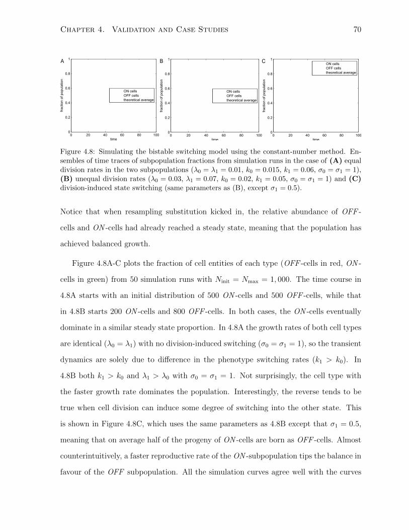
Chapter 4. Validation and Case Studies 70
0 20 40 60 80 1000
0.2
0.4
0.6
0.8
1
time
frac
tion
of p
opul
atio
n
ON cellsOFF cellstheoretical average
0 20 40 60 80 1000
0.2
0.4
0.6
0.8
1
time
frac
tion
of p
opul
atio
n
ON cellsOFF cellstheoretical average
0 20 40 60 80 1000
0.2
0.4
0.6
0.8
1
time
frac
tion
of p
opul
atio
n
ON cellsOFF cellstheoretical average
A B C
Figure 4.8: Simulating the bistable switching model using the constant-number method. En-sembles of time traces of subpopulation fractions from simulation runs in the case of (A) equaldivision rates in the two subpopulations (λ0 = λ1 = 0.01, k0 = 0.015, k1 = 0.06, σ0 = σ1 = 1),(B) unequal division rates (λ0 = 0.03, λ1 = 0.07, k0 = 0.02, k1 = 0.05, σ0 = σ1 = 1) and (C)division-induced state switching (same parameters as (B), except σ1 = 0.5).
Notice that when resampling substitution kicked in, the relative abundance of OFF -
cells and ON -cells had already reached a steady state, meaning that the population has
achieved balanced growth.
Figure 4.8A-C plots the fraction of cell entities of each type (OFF -cells in red, ON -
cells in green) from 50 simulation runs with Ninit = Nmax = 1, 000. The time course in
4.8A starts with an initial distribution of 500 ON -cells and 500 OFF -cells, while that
in 4.8B starts 200 ON -cells and 800 OFF -cells. In both cases, the ON -cells eventually
dominate in a similar steady state proportion. In 4.8A the growth rates of both cell types
are identical (λ0 = λ1) with no division-induced switching (σ0 = σ1 = 1), so the transient
dynamics are solely due to difference in the phenotype switching rates (k1 > k0). In
4.8B both k1 > k0 and λ1 > λ0 with σ0 = σ1 = 1. Not surprisingly, the cell type with
the faster growth rate dominates the population. Interestingly, the reverse tends to be
true when cell division can induce some degree of switching into the other state. This
is shown in Figure 4.8C, which uses the same parameters as 4.8B except that σ1 = 0.5,
meaning that on average half of the progeny of ON -cells are born as OFF -cells. Almost
counterintuitively, a faster reproductive rate of the ON -subpopulation tips the balance in
favour of the OFF subpopulation. All the simulation curves agree well with the curves

Chapter 4. Validation and Case Studies 71
of the expectations, f0(t) and f1(t), given in black, indicating that constant-number
method does reproduce an accurate demographic composition of a temporally changing
population with replicative competition.
Next, we investigate how the variability in the phenotype distributions obtained by
simulation scale with Nmax. Starting with the same initial conditions, the random sub-
stitutions of the constant-number method contribute to the variability between realiza-
tions; however, if the sample population is sufficiently big, its composition—averaged over
realizations—should match the theoretical composition that corresponds to an infinitely
large population (in this case, f0(t), f1(t)). Figure 4.9 shows the fraction of ON -cells in
the simulation over time for A) Nmax = 100, B) Nmax = 1000, and C) Nmax = 5000,
each with Ninit = Nmax. Plotted is the ensemble-average trajectory of 20 runs with a
1-standard deviation envelope. Clearly, as the size of the constant-number sample popu-
lation increases, the variance diminishes and the composition converges to the theoretical
value. Figure 4.9D shows that the root mean square error of F1 at balanced growth scales
as 1/√Nmax, which is the same way fluctuations in the Xi would scale with the total num-
ber of cells N when not using the constant-number method [55]. For a given Nmax, the
variance stays roughly constant and the average simulation trajectory does not appear to
diverge over time from the theoretical average trajectory, suggesting that, in this model,
the resampling substitutions do not produce any error propagation over time.
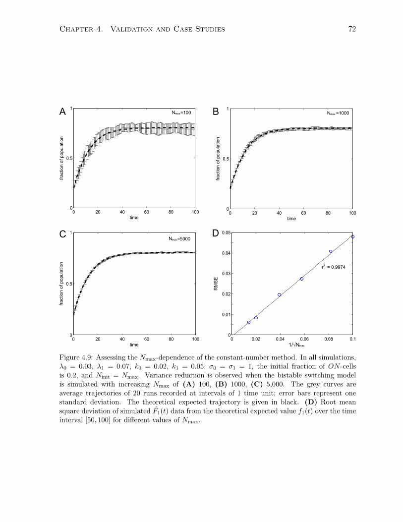
Chapter 4. Validation and Case Studies 72
0 20 40 60 80 1000
0.5
1
time
frac
tion
of p
opul
atio
n
=100
0 20 40 60 80 1000
0.5
1
time
frac
tion
of p
opul
atio
n
=5000
0 20 40 60 80 1000
0.5
1
timefr
actio
n of
pop
ulat
ion
=1000
0 0.02 0.04 0.06 0.08 0.10
0.01
0.02
0.03
0.04
0.05
RM
SE
r2 = 0.9974
1/√N
A B
C D
max
maxN
maxN maxN
Figure 4.9: Assessing the Nmax-dependence of the constant-number method. In all simulations,λ0 = 0.03, λ1 = 0.07, k0 = 0.02, k1 = 0.05, σ0 = σ1 = 1, the initial fraction of ON -cellsis 0.2, and Ninit = Nmax. Variance reduction is observed when the bistable switching modelis simulated with increasing Nmax of (A) 100, (B) 1000, (C) 5,000. The grey curves areaverage trajectories of 20 runs recorded at intervals of 1 time unit; error bars represent onestandard deviation. The theoretical expected trajectory is given in black. (D) Root meansquare deviation of simulated F1(t) data from the theoretical expected value f1(t) over the timeinterval [50, 100] for different values of Nmax.

Chapter 4. Validation and Case Studies 73
4.3 Size and replicative lifespan in budding yeast
4.3.1 Background
The existence of a limit of the number of cellular divisions, referred to as replicative aging,
is common to somatic metazoan cells and yeast cells. In non-immortalized mammalian
cell cultures, cells eventually reach a maximum number of divisions called the Hayflick
limit, and the whole population eventually dies [96]. By contrast, in the budding yeast
Saccharomyces cerevisiae, mother cells eventually cease to replicate while virgin daughter
cells are constantly produced, so the whole population is immortal. Currently, a number
of theories explaining the replicative lifespan—the number of cell divisions a cell achieves
during its lifetime—of budding yeast have been proposed.
Unlike other eukaryotes, S. cerevisiae cells divide by budding, where a smaller daugh-
ter cell emerges from the mother cell as an independent compartment at the beginning
of S-phase and pinches off at the end of the cell cycle. The asymmetry in this replication
mechanism is thought to underlie the finite life span of individual yeast cells. An early
theory held that division capacity was limited due to the formation of bud scars over the
surface of the mother cell, but this was later dismissed by the observation that growth
more than compensates for the loss of surface area due to scarring [45]. The most popu-
lar theory today postulates that some diffusible cytoplasmic “senescence factor” that is
asymmetrically inherited by mother and daughter cell is responsible for aging. Though it
has not yet been identified, some candidates include self-replicating extra-chromosomal
ribosomal DNA circles that accumulate in the mother cell during the budding process,
oxidized proteins, and damaged mitochondria [97].
One recent study on growth and aging in isogenic populations of budding yeast cells
suggested that the replicative lifespan of yeast is limited by the progressive increase in
volume due to asymmetric cell division [98]. The authors used three popular standard

Chapter 4. Validation and Case Studies 74
G1 S G2 M G1 S G2 M
G1 S G2 M G1 S G2 M
m divisions
n<m divisions
senescent
mother cellwildtype
mutant
Figure 4.10: Theory of the size-limited replicative aging of budding yeast. A cell begins growingin G1 phase. Entry into S-phase is accompanied by bud formation. During S-phase growthprimarily occurs in the bud, which separates after mitosis. Progressive increase in the size ofthe mother continues until reaching a critical size at which it cannot re-enter the cell cycle andbecomes senescent. A hypothesized delay at the G1-S checkpoint that does not halt volumegrowth is depicted in red. Based on figure in Zadrag-Tecza et al. [98].
laboratory strains and mutant variants of those strains with various defects in antioxidant
enzymes. Each pair of wild-type and mutant strains demonstrated a cessation of budding
after reaching the same final volume, but had different replicative lifespans. Based on
this and a previous study that used mating pheromone to inhibit budding but not volume
growth [99], the authors propose that a genetically determined critical cell volume may
be the main factor limiting the ability of mother yeast cells to accomplish a successful
cell cycle. They explain that progressive growth of cell volume with each cycle is an
unavoidable consequence of the mechanism of reproduction, because the mother cell
experiences incremental growth during each G1 phase, before a new bud has even formed
(see Figure 4.10). In the mutant cells, oxidative stress leading to DNA damage, would
presumably cause delays at cell cycle at checkpoints without hampering volume growth,
so that mutants attain the limiting cell volume after a smaller number of cell divisions.
A more recent study [100] supports the above findings. The authors looked at a
series of small-size, large-size and “longevity” mutant strains of yeast and observed the

Chapter 4. Validation and Case Studies 75
same relationship between cell size and replicative lifespan. They found that cells that
underwent fewer replications accrued more volume per generation and vice versa, reaching
senescence at a similar maximal volume.
4.3.2 Model
Because the exact relationship between cell volume and the timing of S-phase entry and
bud emergence, as well as the rates of volume growth of the unbudded mother and the bud
at different stages of the cell cycle are poorly understood, we stick to a phenomenological
model of growth that reproduces two observations:
1. The mother cell increases in volume after each division cycle [45],
2. The buds of older mothers tend to be larger [101].
While the studies described suggest that mother cell volume increases steadily with each
generation, little is known about how fast volume accumulates over chronological time,
so we make an arbitrary assumption. Gross (non-compartmentalized) cell volume growth
was assumed to be linear at a given age (generation) and was modelled using V (t) =
V (t− 1) + δv, where δv was obtained (for fixed time step δt = 1) using
δv =kg
1 +(gk
)2 δt, (4.14)
where k is the maximal growth rate and g is the generation (number of buds produced).
Thus, the growth rate is non-monotonic with age, increasing when the cell is younger,
and tending to slow at old age. Cells divide asymmetrically, producing an “older” mother
and a “virgin” daughter from the bud (g = 0). At each division, the daughter receives
a fixed fraction (β) of the gross parental cell volume, while the mother receives the
remaining fraction (1 − β). Division was set to occur every time a pre-specified (strain
specific) volume increment ∆V was reached. When a critical volume is achieved after

Chapter 4. Validation and Case Studies 76
cell division (Vcrit), a cell is flagged as senescent and ceases to proliferate (i.e., it can not
re-enter the cell cycle).
4.3.3 Results and discussion
Figure 4.11A shows the history of a single mother cell’s volume increasing over time.
The periodic decrements are due to the budding off of daughter cells, which gradually
get successively larger as well. When the mother cell volume crosses Vcrit after division,
it ceases to grow. Figure 4.11B presents a plot of gross cell volume as a function of
generation. Different values of k and ∆V were chosen to produce results that mirrored
the experimental results of Zadrag-Tecza et al. [98]. For the wild-type BY4741 strain
k = 4.6 and ∆V = 12µm3, and for the ∆prx antioxidant defective mutant strain k = 1.15
and ∆V = 42.3µm3. Both strains have a similar initial volume at age g = 0, but the
mutant strain accrues volume at a faster rate. Because cells of both strains attain the
same maximal volume, the mutant strain displays a shorter life-span. The data fits well
to a linear trend as did the experimental results.
Figures 4.11 C and D are used to demonstrate an important result about simulating
populations versus simulating ensembles of random cell chains. Figure 4.11C is the
steady state gross cell volume distribution obtained from a simulation of 10,000 random
cell chains. Simulating random cell chains in CPS is achieved simply by not producing
or storing the extra newborn cell when a cell divides. A random cell chain means that
at every division, there is a 50:50 chance of following the mother or the daughter cell.
Figure 4.11D is the same distribution from a population simulation using resampling
substitution with Ninit = Nmax = 10, 000. Notice that the distributions are similar except
for a second peak in 4.11C. This extra peak is an artifact that emerges as a result of slowly
growing old cells and post-mitotic senescent cells that do not get out-competed by younger
cells as they would in a population simulation, as can be seen in the age distributions

Chapter 4. Validation and Case Studies 77
0 100 200 300 400
50
100
150
200
250
Time Step
Vol
ume
(µm
3 )
Mother Cell (∆prx)Vcrit
0 5 10 15 20 25 30 350
50
100
150
200
250
Generations
Vol
ume
(µm
3 )
Mutant (∆prx)Wild Type (BY4741)Linear Regression
0 25 50 75 100 125 150 175 200 225 2500
500
1000
1500
2000
Volume (µm3)
Num
ber
of C
ells
0 25 50 75 100 125 150 175 200 225 2500
500
1000
1500
2000
Volume (µm3)
Num
ber
of C
ells
0 5 10 150
6000
age (generations)
0 5 10 150
6000
age (generations)
R2 = 0.99
R2 = 0.98
A B
C D
Figure 4.11: Simulating size-dependent replicative aging in budding yeast. (A) Time courseof the gross volume of a single mother cell undergoing successive divisions until senescence.(B) Cell volume as a function of age in population simulations of wild-type and shorter-livingmutant strains. (C,D) Steady state cell volume distributions from (C) ensemble simulation ofcell chains and (D) population simulation using the constant-number method. Age distributionsare inset.
Chapter 4. Validation and Case Studies 78
(inset). The distributions obtained by a random cell chain approach are biased towards
states of slower growth because cell chains remain in them for long periods without
competition from fast replicators; senescence is an extreme case of an “absorbing” state
because once entered, the cell ceases to change or divide. This highlights the importance
of using the appropriate simulation methodology.
4.4 Epigenetic memory in the response to stress
4.4.1 Background
Organisms need to cope with a wide variety of environmental changes over a wide range
of time scales. At the cellular level, gene expression patterns and programs have evolved
to prepare for unknown challenges and respond to stress conditions. For example, cells
maintain a fine balance between stress-related and growth-related gene expression pro-
grams, which are regulated by different signalling pathways and tend to have antagonistic
physiological functions [102].
The fact that transcriptional dynamics can be tuned via hard-wired DNA regulatory
elements suggests that expression noise is an evolvable trait [11], and much investigation
has been conducted on how gene expression noise could be exploited to generate adaptive
population variation to deal with environmental stress. This implies the use of gambling
or bet-hedging strategies as a less costly alternative to investing in more precise sense-
response mechanisms [9]. In support of this idea, promoters of stress-related genes tend
to contain a TATA-box, an element which imparts not only faster transcription upon
induction, but noisier expression [103, 104].
One group [105] tested the effect of noise on stress by introducing targeted promoter
mutations to modulate transcriptional bursting in the expression of ZeoR, a protein con-
ferring resistance to the antibiotic Zeocin. They compared the fitness of two strains with

Chapter 4. Validation and Case Studies 79
low and high cell-cell variation in expression but similar mean level, as evinced by flow
cytometry distributions. It was found that the strain with greater heterogeneity pro-
vided a selective advantage at high stress levels, while the less heterogeneous strain had
greater fitness under low levels of stress. Theoretical models were used to explain the
results by imagining different stress thresholds on the reproductive fitness of the popu-
lation [11, 105], where cells expressing below the threshold perish and those expressing
above the threshold are unaffected (see Figure 4.12A). When the stress level is low, a
greater fraction of the low-noise strain can survive and reproduce (represented by the
shaded areas), whereas when the stress level is high, the high-noise strain emerges as the
more fit.
However, this conclusion suffers from the implicit assumption that the expression
levels in the cells (and any offspring produced) are static over the time scale of stress
exposure; it ignores the temporal variability in single cells. Fluctuations in gene expres-
sion can occur over a wide range of timescales—while intrinsic transcriptional bursting
may occur on the order of milliseconds to minutes, extrinsic sources of variation can lead
to long range fluctuations with timescales on the order of the cell cycle [107, 108]. The
notion of a fluctuation timescale in gene expression is sometimes referred to as epigenetic
memory in the physics literature. Note that this definition differs from the more common
use of the term by geneticists and molecular biologists. Memory in the sense defined here
can be quantified as the autocorrelation in an expression time series; thus another term
for memory is “coloured” noise to contrast it with “white” noise in which fluctuations
produce no temporal correlations. Figure 4.12 illustrates how the expression memory of a
single gene in individual cells is hidden when observing the population snapshot. Expres-
sion could be varying rapidly in which cells visit the full range of phenotypes available
to them over the experimental timescale, or it may be fluctuating slowly, in which each
cell has a stable individuality (high degree of memory), which may be heritable. The
conclusion of the model in 4.12A, which does not take memory into account, is only valid
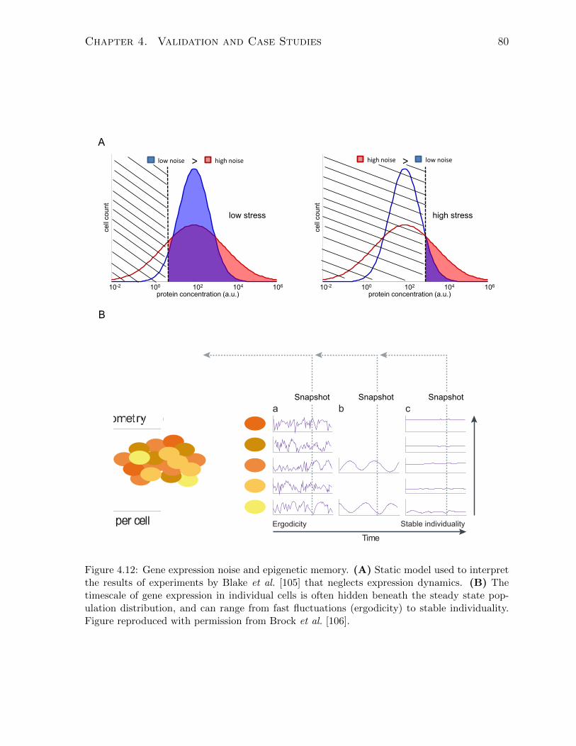
Chapter 4. Validation and Case Studies 80
10-2 100 102 104 106
protein concentration (a.u.)
cell
coun
t
10-2 100 102 104 106
protein concentration (a.u.)
cell
coun
t
low noise high noise> high noise > low noise
A
B
low stress high stress
a b c
Time
Ergodicity Stable individuality
Snapshot Snapshot Snapshot
Figure 4.12: Gene expression noise and epigenetic memory. (A) Static model used to interpretthe results of experiments by Blake et al. [105] that neglects expression dynamics. (B) Thetimescale of gene expression in individual cells is often hidden beneath the steady state pop-ulation distribution, and can range from fast fluctuations (ergodicity) to stable individuality.Figure reproduced with permission from Brock et al. [106].
Chapter 4. Validation and Case Studies 81
at the limit of severe and acute stress (where the unfit cells are instantaneously killed),
or at the limit of infinite memory (where cells do not change expression).
A recent study in S. cerevisiae used a tunable synthetic gene network to produce
populations with different distributions of a URA3-reporter fusion protein [109]. In the
presence of the drug 5-fluoroorotic acid (FOA), the Ura3p enzyme produces a toxic
metabolite 1. Under prolonged exposure to FOA, in some cases the protein distribution
was observed to shift in the direction of lower toxicity, as shown in Figure 4.13. The
“adaptive drift” was reversible, returning to pre-treatment levels upon removal of FOA.
It was hypothesized that epigenetic memory could have been responsible for the observed
dynamic response to imposed stress. Moreover, a similar role for epigenetic memory has
been hypothesized to be contribute to the emergence of drug resistance in cancer cell
populations [106].
In this section, a model of coloured gene expression is developed to assess the adaptive
effect of different expression timescales under long-term stress exposure.
4.4.2 Model
We use a continuous stochastic process called an Ornstein-Uhlenbeck (OU) process as
a phenomenological model of stochastic expression of a single gene product with a tun-
able memory parameter. An OU process x(t) is a continuous, mean-reverting stochastic
process that can be represented using the stochastic differential equation:
x(t+ dt) = x(t)− 1
τ(µ− x(t))dt+
√c dW (t), (4.15)
where µ is the mean level, and dW (t) is a temporally uncorrelated normal random variable
with mean 0 and variance dt called a Wiener process. The OU process can also be
1Hence, in contrast to the previous experiment that dealt with a drug-resistance gene, here lowergene expression is beneficial

Chapter 4. Validation and Case Studies 82
A B C
Figure 4.13: Adaptive drift of URA3GFP-expressing yeast cell populations under prolongedexposure to stress. The strain expresses URA3GFP driven by an rtTA-responsive promoter.rtTA is driven by a Pgal promoter so that its expression is modulated using galactose, whileits activity is modulated using doxycycline, allowing the steady-state expression Ura3pGFP
distribution to be tuned. The flow cytometry distributions show the counts of viable cellsat different times following the exposure to FOA. (A) A low-expressing population incurs aslight drift to lower expression levels, with most cells remaining viable. (B) A population withmoderate expression experiences a dramatic change, undergoing a bimodal transition in whichthe high expression peak diminishes and a low-expressing subpopulation emerges. (C) A high-expressing population is subjected to high levels of stress and the population declines over time.Figure used with permission from Zhuravel et al. [109].
expressed using the Langevin form more familiar to physicists and engineers:
dx(t)
dt=
1
τ(µ− x(t)) +
√c ξ(t), (4.16)
where ξ(t) is Gaussian white noise (〈ξ(t)〉 = 0, 〈ξ(t)ξ(t′)〉 = δ(t)). The parameter τ
is called the relaxation time, and c is called the diffusion constant [110]. The diffusion
constant determines the strength of random fluctuations, while the relaxation time de-
termines how rapidly on average a fluctuation will dissipate back to the mean (i.e the
time scale of fluctuation). The stationary probability distribution of an OU process is a
Gaussian or normal distribution with mean µ and variance cτ/2. The OU process thus
allows us to impose a fixed degree of heterogeneity (the shape and size of the stationary
distribution) and observe the effect of varying the degree of epigenetic memory simply
by modulating the values of c and τ as illustrated in Figure 4.14.
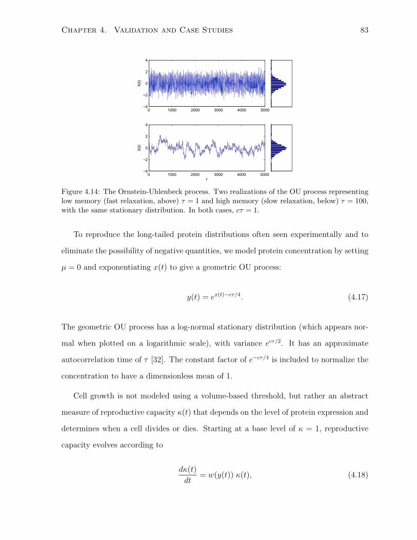
Chapter 4. Validation and Case Studies 83
0 1000 2000 3000 4000 5000−4
−2
0
2
4
X(t)
0 1000 2000 3000 4000 5000−4
−2
0
2
4
t
X(t)
Figure 4.14: The Ornstein-Uhlenbeck process. Two realizations of the OU process representinglow memory (fast relaxation, above) τ = 1 and high memory (slow relaxation, below) τ = 100,with the same stationary distribution. In both cases, cτ = 1.
To reproduce the long-tailed protein distributions often seen experimentally and to
eliminate the possibility of negative quantities, we model protein concentration by setting
µ = 0 and exponentiating x(t) to give a geometric OU process:
y(t) = ex(t)−cτ/4. (4.17)
The geometric OU process has a log-normal stationary distribution (which appears nor-
mal when plotted on a logarithmic scale), with variance ecτ/2. It has an approximate
autocorrelation time of τ [32]. The constant factor of e−cτ/4 is included to normalize the
concentration to have a dimensionless mean of 1.
Cell growth is not modeled using a volume-based threshold, but rather an abstract
measure of reproductive capacity κ(t) that depends on the level of protein expression and
determines when a cell divides or dies. Starting at a base level of κ = 1, reproductive
capacity evolves according to
dκ(t)
dt= w(y(t)) κ(t), (4.18)

Chapter 4. Validation and Case Studies 84
where w(y) is the expression-dependent fitness or reproductive rate function, which is a
sigmoidal Hill-type function of the form
w(y) =wmax + wmin( y
Kw)n
1 + ( yKw
)n, (4.19)
where wmin and wmax are the minimum and maximum reproductive rates, Kw is the Hill
constant, and n the Hill coefficient. The reproductive rate tends to wmax when expression
is low and falls to wmin when expression is sufficiently high as a result of the metabolic
stress caused by the protein. The steepness and midpoint of the curve of the fitness
function w(y) can be changed by modifying the Hill parameters. When κ(t) reaches a
threshold value of 2, the cell divides. However, κ(t) may decrease due to stress if wmin
is negative, and if a cell’s capacity falls below a threshold of 0.5, the cell is flagged as
dead or nonviable. In the simulation experiments presented, division events are perfectly
symmetric: the daughter cells have a reproductive capacity reset to 1 and both inherit
the parental protein concentration (no partitioning error or asymmetry). The time unit
of the model is set to be equal to the generation time (tD)—the time is takes a cell’s
reproductive capacity to double—in the absence of stress (i.e., tD = ln(2)/wmax).
The model was implemented using three local simulation channels: one for repro-
ductive capacity, one for the time evolution of protein concentration (simulated using a
numerically exact method [110]), and one time-driven channel to detect the crossing of
division or death thresholds and respond accordingly. A global simulation channel was
also included to turn on or off a global boolean variable stress, which corresponds to the
addition or removal of FOA to the system. Finally, another global simulation channel
was used to record data at regular intervals. The initial and maximum ensemble size
used in the simulations was 10, 000.

Chapter 4. Validation and Case Studies 85
4.4.3 Results and discussion
Simulations were first conducted to demonstrate the flow of the population distribution in
the response to stress. Beginning with two different populations in the absence of stress
expressing URA3GFP at steady state, stress is induced after t = 0 and the distribution
of viable cells is tracked over time. Figure 4.15 shows the effect of different degrees
of expression memory. In the first population, the expression relaxation time is short:
τ = 0.1 or 10% of the stress-free cell generation time. In the second case τ = 15, so
cells have higher expression memory. The value of the diffusion constant c is adjusted so
that the stress-free distributions have the same shape. The reproductive rate curves in
the simulations shown (green dashed curves) have Hill constant Kw = 0.1 with a steep
threshold n = 10.
Figure 4.15A shows that in the low-memory population, the number of viable cells
diminishes over time and the population goes extinct by around 40 generations. On the
other hand, in the high-memory population (Figure 4.15B), the expression distribution
shifts to the left over time, producing a bimodal transient before settling to a new steady
state. As a result, the population persists in the face of chronic stress. This occurs
because cells in with lower URA3GFP expression levels tend to remain fit for a long
enough period to reproduce. In the low-memory case, cells are rarely able to recover
their reproductive capacity due to rapid gene expression fluctuations and eventually die.
Note that the profile of population drift is sensitive to the steepness of the reproductive
rate function (i.e., the Hill coefficient or “cooperativity” n) and its the position of its
half-saturation value (i.e., the Hill constant Kw). In Figure 4.16A and B, the half-
saturation point of the fitness curve is set at expression values of 0.05 and 0.5, respectively,
with τ = 10 and n = 10. In 4.16A, a small subpopulation maintains viability after 40
generations, while when the stress is less severe (4.16B) the population shift is minor.
Figure 4.16C and D show simulations with a steep n = 10 and soft n = 2 threshold,

Chapter 4. Validation and Case Studies 86
0
10−2
10−1
100
101
102
0
50
100
150
200t=0
0
10−2
10−1
100
101
102
0
50
100
150
200t=10
0
10−2
10−1
100
101
102
0
50
100
150
200t=15
0
10−2
10−1
100
101
102
0
50
100
150
200t=20
0
10−2
10−1
100
101
102
0
50
100
150
200
0
10−2
10−1
100
101
102
0
50
100
150
200
0.35
0.7
Cel
l cou
nt
Protein level (a.u.)
repr
oduc
tive
rate
t=0
0
10−2
10−1
100
101
102
0
50
100
150
200t=25
0
10−2
10−1
100
101
102
0
50
100
150
200
t=30
0
10−2
10−1
100
101
102
0
50
100
150
200t=35
0
10−2
10−1
100
101
102
0
50
100
150
200t=40
A Bτ = 1 τ = 15
t=40
0.35
0.7
0.35
0.7
0.35
0.7
0.35
0.7
0.35
0.7
0.35
0.7
0.35
0.7
0.35
0.7
0.35
0.7
Cel
l cou
nt
Protein level (a.u.)
repr
oduc
tive
rate
Cel
l cou
nt
Protein level (a.u.)
repr
oduc
tive
rate
Cel
l cou
nt
Protein level (a.u.)
repr
oduc
tive
rate
Cel
l cou
nt
Protein level (a.u.)
repr
oduc
tive
rate
Cel
l cou
nt
Protein level (a.u.)
repr
oduc
tive
rate
Cel
l cou
nt
Protein level (a.u.)
repr
oduc
tive
rate
Cel
l cou
nt
Protein level (a.u.)
repr
oduc
tive
rate
Cel
l cou
nt
Protein level (a.u.)
repr
oduc
tive
rate
Cel
l cou
nt
Protein level (a.u.)
repr
oduc
tive
rate
Figure 4.15: Slower relaxation of fluctuations causes adaptive drift of the population expressiondistribution under stress and confers resistance. Starting at steady-state in the absence ofstress, stress is introduced at t = 0 and the distribution of viable cells is followed over time.The parameters of the reproductive rate function are n = 10 and Kw = 0.1. (A) Memoryis on the order of a single generation time τ = 1. (B) Memory is significantly longer than ageneration τ = 15.

Chapter 4. Validation and Case Studies 87
respectively, with τ = 10 and Kw = 0.1. As the threshold is made softer, the extent
of drift appears and the intermediate bimodal distribution tend to diminish and give
rise to a broader stationary distribution under stress. The lower panels show the effect
of removing the stress at t = 40. Importantly, expression distributions always migrate
back to the original steady-state distribution once stress is removed, as was observed
experimentally [109]. The migration occurs with no bimodal transition.
Figure 4.17 shows a plot of the drift in the mean level of Ura3pGFP following stress
introduction and after its subsequent removal for different degrees of expression memory.
The curves show the average and standard deviations of 10 runs for each set of parameters.
The greater the relaxation time, the greater the extent of drift in mean expression. Note
that the return of the mean to the pre-stress value appears to follow an exponential
relaxation whose relaxation rate is roughly the memory parameter τ . This suggests that
the monotonic relaxation of the expression peak in the absence of stress could be used
experimentally as an empirical measure of the degree of epigenetic memory. A more direct
measure of memory has been employed in live cell microscopy experiments of YFP -tagged
proteins at different chromosomal loci of human cells [111]. There, the time it takes for
a cell lineage to reach the different states found in a snapshot of a cell population was
measured via the “mixing time” or the time at which the auto-correlation decays to half
its initial value. It would be interesting to see how well lineage- and population-based
experimental measurements of epigenetic memory agree.
Compare the simulation results with the experimental data of Zhuravel et al. shown
in Figure 4.13, in which memory was not measured and could not be directly controlled,
but instead the level of expression was varied. In the cases of cells induced at low
and intermediate levels prior to stress introduction, the distribution settled to a similar
final position under stress. In the case of cells induced to high pre-stress levels, the
population died out, likely because expression levels cannot manage to drift to safer levels
before toxicity sets in (in fact, the small visible subpopulation on the left is reminiscent

Chapter 4. Validation and Case Studies 88
0
10−2
10−1
100
101
102
0
50
100
150
200
Cel
l cou
nt
Protein level (a.u.)
t=0t=20t=40
0
10−2
10−1
100
101
102
0
50
100
150
200
Cel
l cou
nt
Protein level (a.u.)
t=40t=45t=50t=80
0
10−2
10−1
100
101
102
0
50
100
150
200
Cel
l cou
nt
Protein level (a.u.)
t=0t=20t=40
0
10−2
10−1
100
101
102
0
50
100
150
200
Cel
l cou
nt
Protein level (a.u.)
t=40t=45t=50t=80
C D
0
0.35
0.7
repr
oduc
tive
rate
10−2
10−1
100
101
102
0
50
100
150
200
Cel
l cou
nt
Protein level (a.u.)
t=0t=20t=30t=40
0
10−2
10−1
100
101
102
0
50
100
150
200
Cel
l cou
nt
Protein level (a.u.)
t=0t=20t=30t=40
A B
0.35
0.7
repr
oduc
tive
rate
0.35
0.7
repr
oduc
tive
rate
0.35
0.7
repr
oduc
tive
rate
0.35
0.7
repr
oduc
tive
rate
0.35
0.7
repr
oduc
tive
rate
Kw = 0.05n = 10
Kw = 0.5n = 10
Kw = 0.1n = 10
Kw = 0.1n = 2
Figure 4.16: Varying the position and steepness of the reproductive rate function (green). (A,B)The Hill constant Kw is set at 0.05 and 0.5, respectively. (C,D) The Hill coefficient n is 10and 2, respectively. The migration of the distributions back to their initial position followingremoval of stress is given in the panels below.

Chapter 4. Validation and Case Studies 89
0 10 20 30 40 50 60 70 800
0.2
0.4
0.6
0.8
1
Figure 4.17: Reversible adaptive drift of mean URA3GFP expression for different values of τ .Curves give the average over 10 simulation runs with error bars measuring standard deviation.In all cases, n = 2 and Kw = 0.1. The rate of return to the initial level following FOA removalis related to the degree of memory τ .
of Figure 4.16A). The simulation study here suggests that slow fluctuation in protein
expression may indeed be the primary factor responsible for the population dynamics
observed.

Chapter 5
Conclusion
A general simulation framework has been presented that facilitates the development and
execution of individual-based population dynamics simulations of biological cells. This is
done by using modular and reusable objects called simulation channels which encapsulate
separate state-updating algorithms. Given a complete set of simulation channels and an
initial population state, a simulation run is conducted using one of two scheduling pro-
tocols (the meta-algorithms) that make use of user-specified channel interdependencies.
These protocols ensure the correct execution sequence of simulation events and are de-
signed to minimize or eliminate redundant rescheduling of channels. They also ensure the
correct random substitution of newborn cells after a maximum number of cell entities is
obtained. With this constant-number method, simulations can be run for arbitrarily long
times, allowing the sample population to reach a state of balanced growth or steady-state
composition. Furthermore, the framework permits the recording of multivariate snap-
shots of the ensemble of cell entities at scheduled times, or the recording of single-cell
histories, allowing the construction of cell lineage trees. A series of modeling studies were
presented to validate the framework implementation and to provide realistic use cases.
Simulation channels can be a very useful tool for model development; however, a
90

Chapter 5. Conclusion 91
few limitations and drawbacks exist. For instance, one side-effect of defining models in
terms of simulation channels is that this places the semantics of the biological model
and its simulation on the same level, so that the model cannot be easily abstracted
away from the simulation algorithms [84]. While there are disadvantages to this kind of
formalism, it can also be an insightful way to decompose and analyze a dynamic system
with complicated structure and to track down bugs. However, the primary limitation of
the framework stems from the insulation of simulation channels from one another. In the
current design, simulation channels—even those contained in the same engine—do not
share information directly with one another. They can only coordinate their execution
through the pre-defined rescheduling dependency graph or by passing information to one
another indirectly by reading and modifying the state data of a common entity. This
leads to the perhaps undesirable consequence of sometimes using cell entity or global state
data as flags or variables for simulation algorithm logic rather than being properties that
lie purely in the domain of the conceptual biological model.
This limitation complicates the simulation of cell-cell interactions and certain global
events. In the current design, it is technically prohibited for a global simulation channel
to modify cell entities directly, and the same goes for local channels and global data.
The reason this should be enforced is that if cell entities could be modified by a global
simulation channel, the manager would not be able to tell whether any cell entities were
modified, and therefore decide, which, if any, local channels need to be rescheduled after
a global event. Conversely, if a local simulation channel were permitted to modify global
state variables, it would not be clear following local channel execution if any global sim-
ulation channels need to be rescheduled. To get around this, scheduling dependencies
between global and local channels could be introduced into the framework, but the re-
sulting relationships would become very complicated and place an undue burden on the
model developer.
Under these restrictions, attempts at introducing direct cell-cell communication in a

Chapter 5. Conclusion 92
model end up being contrived, involving the sending of information from global channels
to local channels indirectly by modifying global state variables and vice versa by modi-
fying local state variables. To resolve this difficulty and avoid the need for local-global
dependencies, it would therefore be desirable to introduce some mechanism by which an
isolated simulation channel may be invoked or rescheduled from within another simulation
channel, rather than relate channels only by pre-defined dependence relationships. This
way one could create, for example, a global simulation channel whose execute method
selects some subset of cells and sends “directives” to execute some of their local simula-
tion channels in order to change those cells; following execution of those local channels,
the corresponding local engines would then be able to invoke the required rescheduling
dependencies immediately. Such a mechanism would also allow local channels of one cell
entity to trigger local channels of another cell entity.
These notification signals or directives would have to be relayed by the simulation
manager, to whom all engines are visible, and it should only be permitted to occur when
the system is synchronized in model time. In sum, a possible extension of the current
framework would involve incorporating a means for the manager to relay messages from
simulation channels to reschedule or perhaps to directly fire other simulation channels,
as illustrated in Figure 5.1. However, if channels can fire one another without advancing
the simulation clock, one must be careful not to accidentally introduce cyclic paths of
channel invocations, as this will create deadlock.
While the framework meta-algorithm automatically initiates resampling substitution
as soon as the number of cells exceeds Nmax, the current design only handles substitution
upon addition (i.e., when new cells are born). The resampling counterpart for the case
of cell death would be to remove a dead cell from the simulation and replace it with a
copy of a randomly chosen cell entity. So far, cell death has been treated as a phenotype:
a “dead” cell is kept as part of the sample population of interest, and can be replaced
by new cells, but the cell entity is inactivated so that its engine ceases to simulate it

Chapter 5. Conclusion 93
Process messages from engines:
M
L G
"fire global channel gi""fire local channel li in engine Lj"
"fire global channel gi""fire local channel li in engine Lj"
1. force-execute channels requested2. reschedule dependent channels
messages: messages:
At synchronization...
Figure 5.1: Possible extension of the framework allowing dynamic dependencies between simu-lation channels, even those in different simulation engines.
(see Appendix A). It is often the case that non-viable cells are part of the “population
of interest” that the simulation is approximating, so this is usually the desired result.
However, in some cases one might want to remove certain cells from the sample population
because they are no longer of interest or because they are being physically destroyed (e.g.,
by necrosis or lysis due to osmotic stress). In those cases, the framework should provide
the option to include resampling substitution upon removal. This would fit easily into the
First-Engine Method version of the simulation meta-algorithm, but we run into difficulty
again with the Asynchronous Method. Since correct substitution requires that the whole
population be synchronized at the precise time the cell is removed, substitution cannot
be triggered by local simulation channels during the asynchronous intervals between time
barriers. Substitution could instead be performed at the next available time barrier, but
unlike the case of substitution for newborns, there is no way to guarantee the consistency
of substitutions of removed cells with those produced by the conservative First-Engine
Method version of the meta-algorithm.
Another property of the constant-number method that was omitted is the fact that

Chapter 5. Conclusion 94
the size or number concentration of the “true” or “total” population can be estimated
and tracked as the simulation proceeds. This is based on the interpretation that each
cell in the constant-number sample population is some sort of representational average
of 1/Nmax of the cells in the total population [112]. In that case, each time a new cell is
born in the sample population, the total population counter Ntotal is incremented by a
proportional amountNmax/Ntotal, and similarly decremented when a cell is removed. Such
a population counter could easily be built into the framework. This is valuable because
estimating macroscopic variables like total cell number, average cell mass, or external
concentrations of signalling molecules directly from the sample population allows one to
simulate indirect cell-cell communication through the environment. For example, one
could simulate density-dependent growth by tying single-cell growth rates of individual
cells to the estimated total population size Ntotal.
The CPS framework is designed around the idea of the constant-number ensemble as a
representative sample of the population of interest. But in what situations is this method
of replacing random individuals valid or meaningful? The constant-number method cre-
ates an ensemble that is structured by the proliferation and death rates of cells, not by
spatial considerations or other special properties attached to cells—unless these have an
affect on growth. In sample populations that are too small, some side-effects of this are
that it is possible for the slowest-proliferating cell types to be completely suppressed due
to constant replacement by newborns or for a population to experience random changes
in composition similar to the phenomena of genetic drift and fixation in population ge-
netics. Such small-number effects are important to keep in mind. If instead of capturing
the composition of all cells, one were more interested, for example, in their spatial organi-
zation, one might want to produce a different kind of ensemble that tracks cells confined
to a spatial area or volume. That would require some different approach to adding or
removing cells from the sample, since cells may now enter or leave the space (e.g., a
spatial lattice with cell-absorbing boundaries or cell reservoirs). It would be interesting

Chapter 5. Conclusion 95
to explore how other entity-management approaches such as this could be combined with
the basic engine-channel architecture described in this thesis.
Finally, although the Asynchronous Method was initially pursued for its parallelism,
clearly models involving a constantly changing environment, consumption of resources,
or cell-cell communication would, in general, require very frequent synchronizations of
the simulation ensemble and preclude any runtime speed-up from parallelization. In
any case, as with all types of experiments, most simulation experiments need to be
reproduced or run multiple times; hence, it is probably ultimately more valuable to be
able to perform multiple simulation runs in parallel rather than to parallelize the running
of a particular realization. Future design work will therefore focus mainly on extending
the framework to better accommodate coupling of local and global simulation events, to
accommodate cell removal and substitution of removed cells, and to provide a built-in
population counter. Furthermore, an efficient version of the current framework design is
currently being implemented in the language C++.

References
[1] Steven J. Altschuler and Lani F. Wu. Cellular Heterogeneity: Do Differences Make
a Difference? Cell, 141(4):559–563, May 2010.
[2] J. E. Ferrell Jr. The Biochemical Basis of an All-or-None Cell Fate Switch in
Xenopus Oocytes. Science, 280(5365):895–898, May 1998.
[3] H Rubin. The significance of biological heterogeneity. Cancer metastasis reviews,
9(1):1–20, July 1990.
[4] Hannah H Chang, Martin Hemberg, Mauricio Barahona, Donald E Ingber, and Sui
Huang. Transcriptome-wide noise controls lineage choice in mammalian progenitor
cells. Nature, 453(7194):544–7, 2008.
[5] A. Raj and A. Van Oudenaarden. Nature, Nurture, or Chance: Stochastic Gene
Expression and Its Consequences. Cell, 135(2):216–226, 2008.
[6] D B Kell, H M Ryder, a S Kaprelyants, and H V Westerhoff. Quantifying het-
erogeneity: flow cytometry of bacterial cultures. Antonie van Leeuwenhoek, 60(3-
4):145–58, 1991.
[7] Carla J Davidson and Michael G Surette. Individuality in bacteria. Annual review
of genetics, 42:253–68, 2008.
96

References 97
[8] A A Cohen, N Geva-Zatorsky, E Eden, M Frenkel-Morgenstern, I Issaeva, A Sigal,
R Milo, C Cohen-Saidon, Y Liron, Z Kam, L Cohen, T Danon, N Perzov, and
U Alon. Dynamic proteomics of individual cancer cells in response to a drug.
Science (New York, N.Y.), 322(5907):1511–6, December 2008.
[9] Edo Kussell and Stanislas Leibler. Phenotypic diversity, population growth, and in-
formation in fluctuating environments. Science (New York, N.Y.), 309(5743):2075–
8, 2005.
[10] Jan-Willem Veening, Wiep Klaas Smits, and Oscar P Kuipers. Bistability, epige-
netics, and bet-hedging in bacteria. Annual review of microbiology, 62:193–210,
2008.
[11] Dawn Fraser and Mads Kaern. A chance at survival: gene expression noise and
phenotypic diversification strategies. Molecular microbiology, 71(6):1333–40, 2009.
[12] A.L. Givan. Flow cytometry: first principles. Wiley-Liss, 2001.
[13] James C W Locke and Michael B Elowitz. Using movies to analyse gene circuit
dynamics in single cells. Nature reviews. Microbiology, 7(5):383–92, 2009.
[14] Diane Longo and Jeff Hasty. Dynamics of single-cell gene expression. Molecular
systems biology, 2:64, 2006.
[15] Ido Golding, Johan Paulsson, Scott M Zawilski, and Edward C Cox. Real-time
kinetics of gene activity in individual bacteria. Cell, 123(6):1025–36, 2005.
[16] Long Cai, Nir Friedman, and X Sunney Xie. Stochastic protein expression in
individual cells at the single molecule level. Nature, 440(7082):358–62, March 2006.
[17] Ji Yu, Jie Xiao, Xiaojia Ren, Kaiqin Lao, and X Sunney Xie. Probing gene ex-
pression in live cells, one protein molecule at a time. Science (New York, N.Y.),
311(5767):1600–3, 2006.

References 98
[18] J Tyson, Katherine C Chen, and Bela Novak. Sniffers, buzzers, toggles and blinkers:
dynamics of regulatory and signaling pathways in the cell. Current Opinion in Cell
Biology, 15(2):221–231, April 2003.
[19] Uri Alon. Network motifs: theory and experimental approaches. Nature reviews.
Genetics, 8(6):450–61, 2007.
[20] John J Tyson and Bela Novak. Functional motifs in biochemical reaction networks.
Annual review of physical chemistry, 61:219–40, March 2010.
[21] Naama Barkai and Ben-Zion Shilo. Variability and robustness in biomolecular
systems. Molecular cell, 28(5):755–60, 2007.
[22] Ernesto Andrianantoandro, Subhayu Basu, David K Karig, and Ron Weiss. Syn-
thetic biology: new engineering rules for an emerging discipline. Molecular systems
biology, 2:2006.0028, 2006.
[23] Priscilla E M Purnick and Ron Weiss. The second wave of synthetic biology: from
modules to systems. Nature reviews. Molecular cell biology, 10(6):410–22, June
2009.
[24] Shankar Mukherji and Alexander van Oudenaarden. Synthetic biology: un-
derstanding biological design from synthetic circuits. Nature reviews. Genetics,
10(12):859–71, 2009.
[25] C.H. Waddington. The strategy of the genes: A discussion of some aspects of
theoretical biology. With an appendix by H. Kacser. London: George Allen &
Unwin, Ltd., 1957.
[26] Gabor Balazsi, Alexander van Oudenaarden, and James J Collins. Cellular decision
making and biological noise: from microbes to mammals. Cell, 144(6):910–25,
March 2011.

References 99
[27] Avigdor Eldar and Michael B. Elowitz. Functional roles for noise in genetic circuits.
Nature, 467(7312):167–173, September 2010.
[28] Mads Kaern, Timothy C Elston, William J Blake, and James J Collins. Stochas-
ticity in gene expression: from theories to phenotypes. Nature reviews. Genetics,
6(6):451–64, 2005.
[29] Arjun Raj, Charles S Peskin, Daniel Tranchina, Diana Y Vargas, and Sanjay Tyagi.
Stochastic mRNA synthesis in mammalian cells. PLoS biology, 4(10):e309, 2006.
[30] Johan Paulsson. Summing up the noise in gene networks. Nature, 427(6973):415–8,
January 2004.
[31] Juan M Pedraza and Alexander van Oudenaarden. Noise propagation in gene
networks. Science (New York, N.Y.), 307(5717):1965–9, 2005.
[32] Vahid Shahrezaei and Peter S Swain. The stochastic nature of biochemical net-
works. Current opinion in biotechnology, 19(4):369–74, August 2008.
[33] Michael B Elowitz, Arnold J Levine, Eric D Siggia, and Peter S Swain. Stochastic
gene expression in a single cell. Science (New York, N.Y.), 297(5584):1183–6, 2002.
[34] P S Swain, M B Elowitz, and E D Siggia. Intrinsic and extrinsic contributions
to stochasticity in gene expression. Proc. Natl. Acad. Sci. USA, 99:12795–12800,
2002.
[35] Gurol M Suel, Rajan P Kulkarni, Jonathan Dworkin, Jordi Garcia-Ojalvo, and
Michael B Elowitz. Tunability and noise dependence in differentiation dynamics.
Science (New York, N.Y.), 315(5819):1716–9, March 2007.
[36] Hedia Maamar, Arjun Raj, and David Dubnau. Noise in gene expression determines
cell fate in Bacillus subtilis. Science (New York, N.Y.), 317(5837):526–9, 2007.

References 100
[37] Murat Acar, Attila Becskei, and Alexander van Oudenaarden. Enhancement of
cellular memory by reducing stochastic transitions. Nature, 435(7039):228–32, May
2005.
[38] Mathias F Wernet, Esteban O Mazzoni, Arzu Celik, Dianne M Duncan, Ian Dun-
can, and Claude Desplan. Stochastic spineless expression creates the retinal mosaic
for colour vision. Nature, 440(7081):174–80, March 2006.
[39] Edward R Sumner and Simon V Avery. Phenotypic heterogeneity: differential
stress resistance among individual cells of the yeast Saccharomyces cerevisiae. Mi-
crobiology (Reading, England), 148(Pt 2):345–51, February 2002.
[40] Dann Huh and Johan Paulsson. Non-genetic heterogeneity from stochastic parti-
tioning at cell division. Nature genetics, 43(2):95–100, February 2011.
[41] Pao-Shu Wu, Boris Egger, and Andrea H Brand. Asymmetric stem cell division:
lessons from Drosophila. Seminars in cell & developmental biology, 19(3):283–93,
June 2008.
[42] Ralph a Neumuller and Juergen a Knoblich. Dividing cellular asymmetry: asym-
metric cell division and its implications for stem cells and cancer. Genes & devel-
opment, 23(23):2675–99, December 2009.
[43] Eric J Stewart, Richard Madden, Gregory Paul, and Francois Taddei. Aging and
death in an organism that reproduces by morphologically symmetric division. PLoS
biology, 3(2):e45, March 2005.
[44] Nathalie Q Balaban, Jack Merrin, Remy Chait, Lukasz Kowalik, and Stanislas
Leibler. Bacterial persistence as a phenotypic switch. Science (New York, N.Y.),
305(5690):1622–5, September 2004.

References 101
[45] S M Jazwinski. Aging and senescence of the budding yeast Saccharomyces cere-
visiae. Molecular microbiology, 4(3):337–43, March 1990.
[46] K C Chen, a Csikasz-Nagy, B Gyorffy, J Val, B Novak, and J J Tyson. Kinetic
analysis of a molecular model of the budding yeast cell cycle. Molecular biology of
the cell, 11(1):369–91, January 2000.
[47] Mukund Thattai and Alexander van Oudenaarden. Stochastic gene expression in
fluctuating environments. Genetics, 167(1):523–30, May 2004.
[48] Edo Kussell, Roy Kishony, Nathalie Q Balaban, and Stanislas Leibler. Bacterial
persistence: a model of survival in changing environments. Genetics, 169(4):1807–
14, 2005.
[49] David Gilbert, Hendrik Fuss, Xu Gu, Richard Orton, Steve Robinson, Vladislav
Vyshemirsky, Mary Jo Kurth, C Stephen Downes, and Werner Dubitzky. Computa-
tional methodologies for modelling, analysis and simulation of signalling networks.
Briefings in bioinformatics, 7(4):339–53, December 2006.
[50] B.B. Aldridge, J.M. Burke, D.A. Lauffenburger, and P.K. Sorger. Physicochemical
modelling of cell signalling pathways. Nature cell biology, 8(11):1195–1203, 2006.
[51] Herbert M Sauro. Network dynamics. Methods in molecular biology (Clifton, N.J.),
541:269, 2009.
[52] Natal a W van Riel. Dynamic modelling and analysis of biochemical networks:
mechanism-based models and model-based experiments. Briefings in bioinformat-
ics, 7(4):364–74, December 2006.
[53] E.D. Conrad and J.J. Tyson. Modeling molecular interaction networks with non-
linear ordinary differential equations. In Zoltan Szallasi, Jorg Stelling, and Vipul
References 102
Periwal, editors, Systems Modelling in Cellular Biology: From Concept to Nuts and
Bolts. MIT Press, Cambridge, MA, 2006.
[54] D.T. Gillespie. A general method for numerically simulating the stochastic
time evolution of coupled chemical reactions. Journal of computational physics,
22(4):403–434, 1976.
[55] N.G. Van Kampen. Stochastic processes in physics and chemistry. North-Holland
personal library. North-Holland, 1992.
[56] Daniel T Gillespie. Stochastic simulation of chemical kinetics. Annual review of
physical chemistry, 58:35–55, 2007.
[57] Daniel T. Gillespie. Exact stochastic simulation of coupled chemical reactions. The
Journal of Physical Chemistry, 81(25):2340–2361, 1977.
[58] Michael A. Gibson and Jehoshua Bruck. Efficient Exact Stochastic Simulation of
Chemical Systems with Many Species and Many Channels. The Journal of Physical
Chemistry A, 104(9):1876–1889, March 2000.
[59] Yang Cao, Linda R Petzold, Muruhan Rathinam, and Daniel T Gillespie. The nu-
merical stability of leaping methods for stochastic simulation of chemically reacting
systems. The Journal of chemical physics, 121(24):12169–78, December 2004.
[60] James M McCollum, Gregory D Peterson, Chris D Cox, Michael L Simpson, and
Nagiza F Samatova. The sorting direct method for stochastic simulation of bio-
chemical systems with varying reaction execution behavior. Computational biology
and chemistry, 30(1):39–49, February 2006.
[61] Alexander Slepoy, Aidan P Thompson, and Steven J Plimpton. A constant-time ki-
netic Monte Carlo algorithm for simulation of large biochemical reaction networks.
The Journal of chemical physics, 128(20):205101, May 2008.

References 103
[62] Marc R Roussel and Rui Zhu. Validation of an algorithm for delay stochastic
simulation of transcription and translation in prokaryotic gene expression. Physical
biology, 3(4):274–84, November 2006.
[63] J Elf and M Ehrenberg. Spontaneous separation of bi-stable biochemical systems
into spatial domains of opposite phases. Cell, 1(2), 2004.
[64] Caroline Lemerle, Barbara Di Ventura, and Luis Serrano. Space as the final fron-
tier in stochastic simulations of biological systems. FEBS letters, 579(8):1789–94,
March 2005.
[65] D.T. Gillespie. Approximate accelerated stochastic simulation of chemically react-
ing systems. The Journal of Chemical Physics, 115(4):1716, 2001.
[66] Jurgen Pahle. Biochemical simulations: stochastic, approximate stochastic and
hybrid approaches. Briefings in bioinformatics, 10(1):53–64, January 2009.
[67] Mads Kaern, William J Blake, and J J Collins. The engineering of gene regulatory
networks. Annual review of biomedical engineering, 5:179–206, 2003.
[68] J. Paulsson and M. Ehrenberg. Noise in a minimal regulatory network: plasmid
copy number control. Quarterly reviews of biophysics, 34(01):1–59, 2001.
[69] J J Tyson and O Diekmann. Sloppy size control of the cell division cycle. Journal
of theoretical biology, 118(4):405–26, February 1986.
[70] Attila Csikasz-Nagy. Computational systems biology of the cell cycle. Briefings in
bioinformatics, 10(4):424–34, July 2009.
[71] Stefan Klumpp, Zhongge Zhang, and Terence Hwa. Growth rate-dependent global
effects on gene expression in bacteria. Cell, 139(7):1366–75, 2009.
[72] Matthew Scott and Terence Hwa. Bacterial growth laws and their applications.
Current opinion in biotechnology, 22(4):559–565, May 2011.
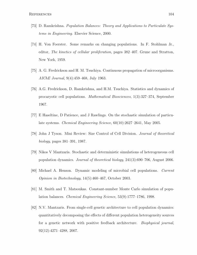
References 104
[73] D. Ramkrishna. Population Balances: Theory and Applications to Particulate Sys-
tems in Engineering. Elsevier Science, 2000.
[74] H. Von Foerster. Some remarks on changing populations. In F. Stohlman Jr.,
editor, The kinetics of cellular proliferation, pages 382–407. Grune and Stratton,
New York, 1959.
[75] A. G. Fredrickson and H. M. Tsuchiya. Continuous propagation of microorganisms.
AIChE Journal, 9(4):459–468, July 1963.
[76] A.G. Fredrickson, D. Ramkrishna, and H.M. Tsuchiya. Statistics and dynamics of
procaryotic cell populations. Mathematical Biosciences, 1(3):327–374, September
1967.
[77] E Haseltine, D Patience, and J Rawlings. On the stochastic simulation of particu-
late systems. Chemical Engineering Science, 60(10):2627–2641, May 2005.
[78] John J Tyson. Mini Review: Size Control of Cell Division. Journal of theoretical
biology, pages 381–391, 1987.
[79] Nikos V Mantzaris. Stochastic and deterministic simulations of heterogeneous cell
population dynamics. Journal of theoretical biology, 241(3):690–706, August 2006.
[80] Michael A. Henson. Dynamic modeling of microbial cell populations. Current
Opinion in Biotechnology, 14(5):460–467, October 2003.
[81] M. Smith and T. Matsoukas. Constant-number Monte Carlo simulation of popu-
lation balances. Chemical Engineering Science, 53(9):1777–1786, 1998.
[82] N.V. Mantzaris. From single-cell genetic architecture to cell population dynamics:
quantitatively decomposing the effects of different population heterogeneity sources
for a genetic network with positive feedback architecture. Biophysical journal,
92(12):4271–4288, 2007.

References 105
[83] D.A. Charlebois, Jukka Intosalmi, Dawn Fraser, and M. Kaern. An Algorithm
for the Stochastic Simulation of Gene Expression and Heterogeneous Population
Dynamics. Commun. Comput. Phys, 9(2011):89–112, 2011.
[84] Kouichi Takahashi, Katsuyuki Yugi, Kenta Hashimoto, Yohei Yamada, Christopher
J F Pickett, and Masaru Tomita. Challenges in Cell Simulation : A Software
Engineering Approach. IEEE Intelligent Systems, 2002.
[85] R.W. Lafore. Object-oriented programming in C++. Kaleidoscope Series. Sams,
2002.
[86] M.A. Weisfeld. The object-oriented thought process. Developer’s library. Sams Pub.,
2004.
[87] R.M. Fujimoto. Parallel and distributed simulation systems. Wiley series on parallel
and distributed computing. Wiley, 2000.
[88] Howard Salis and Yiannis Kaznessis. Accurate hybrid stochastic simulation of
a system of coupled chemical or biochemical reactions. The Journal of chemical
physics, 122(5):54103, 2005.
[89] Johan Paulsson. Models of stochastic gene expression. Physics of Life Reviews,
2(2):157–175, June 2005.
[90] Paul J Choi, Sunney Xie, and Eugene I Shakhnovich. Stochastic switching in gene
networks can occur by a single-molecule event or many molecular steps. Journal
of molecular biology, 396(1):230–44, February 2010.
[91] E M Ozbudak, M Thattai, I Kurtser, A D Grossman, and A Van Oudenaarden.
Regulation of noise in the expression of a single gene. Nat. Genet, 31:69–73, 2002.

References 106
[92] Vahid Shahrezaei and Peter S Swain. Analytical distributions for stochastic gene
expression. Proceedings of the National Academy of Sciences of the United States
of America, 105(45):17256–61, November 2008.
[93] T Lu, D Volfson, and L Tsimring. Cellular growth and division in the Gillespie
algorithm. Syst. Biol, 1(1):121–128, 2004.
[94] E. Renshaw. Birth, Death and Migration Processes. Biometrika, 59(1):49, April
1972.
[95] Eric Renshaw. A survey of stepping-stone models in population dynamics. Advances
in applied probability, 18(3):581–627, September 1986.
[96] J W Shay and W E Wright. Hayflick, his limit, and cellular ageing. Nature reviews.
Molecular cell biology, 1(1):72–6, October 2000.
[97] Kiersten A Henderson and Daniel E Gottschling. A mother’s sacrifice: what is she
keeping for herself? Current opinion in cell biology, 20(6):723–8, December 2008.
[98] Renata Zadrag-Tecza, Magdalena Kwolek-Mirek, Grzegorz Bartosz, and Tomasz
Bilinski. Cell volume as a factor limiting the replicative lifespan of the yeast Sac-
charomyces cerevisiae. Biogerontology, 10(4):481–8, August 2009.
[99] Renata Zadrag, Magdalena Kwolek-Mirek, Grzegorz Bartosz, and Tomasz Bilin-
ski. Relationship between the replicative age and cell volume in Saccharomyces
cerevisiae. Acta biochimica Polonica, 53(4):747–51, January 2006.
[100] Jingye Yang, Huzefa Dungrawala, Hui Hua, Arkadi Manukyan, Lesley Abraham,
Wesley Lane, Holly Mead, Jill Wright, and Brandt L Schneider. Cell size and
growth rate are major determinants of replicative lifespan. Cell cycle (Georgetown,
Tex.), 10(1):144–55, January 2011.
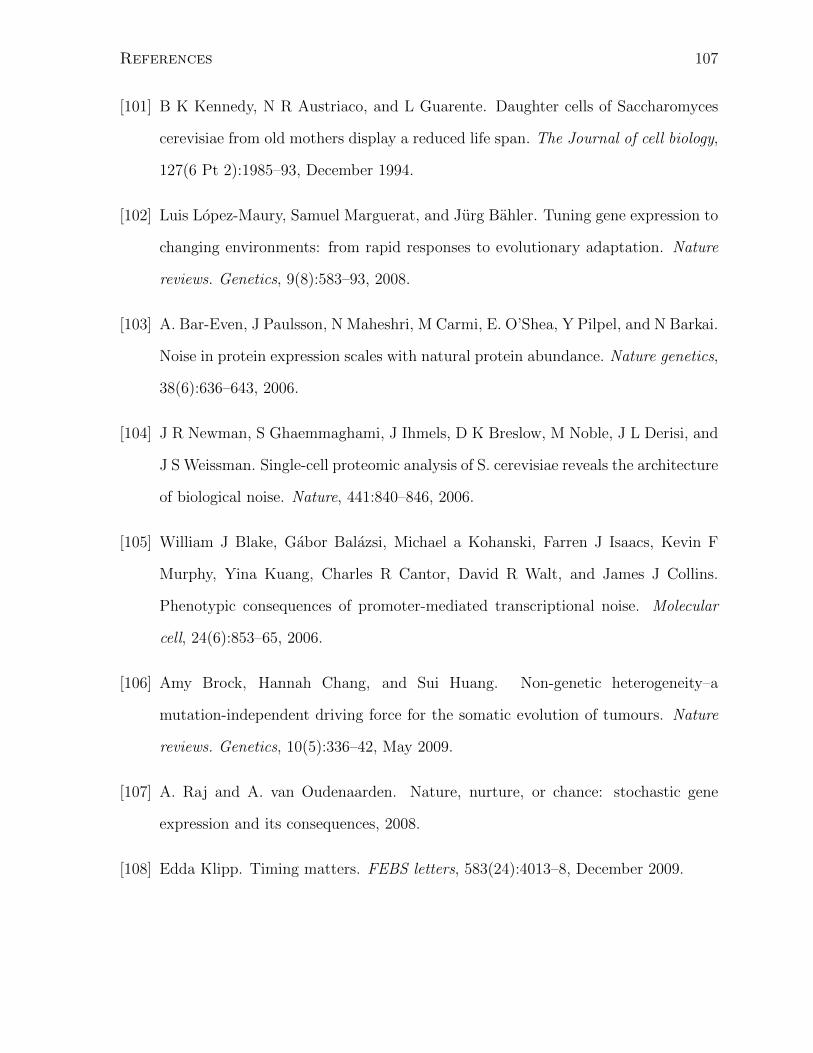
References 107
[101] B K Kennedy, N R Austriaco, and L Guarente. Daughter cells of Saccharomyces
cerevisiae from old mothers display a reduced life span. The Journal of cell biology,
127(6 Pt 2):1985–93, December 1994.
[102] Luis Lopez-Maury, Samuel Marguerat, and Jurg Bahler. Tuning gene expression to
changing environments: from rapid responses to evolutionary adaptation. Nature
reviews. Genetics, 9(8):583–93, 2008.
[103] A. Bar-Even, J Paulsson, N Maheshri, M Carmi, E. O’Shea, Y Pilpel, and N Barkai.
Noise in protein expression scales with natural protein abundance. Nature genetics,
38(6):636–643, 2006.
[104] J R Newman, S Ghaemmaghami, J Ihmels, D K Breslow, M Noble, J L Derisi, and
J S Weissman. Single-cell proteomic analysis of S. cerevisiae reveals the architecture
of biological noise. Nature, 441:840–846, 2006.
[105] William J Blake, Gabor Balazsi, Michael a Kohanski, Farren J Isaacs, Kevin F
Murphy, Yina Kuang, Charles R Cantor, David R Walt, and James J Collins.
Phenotypic consequences of promoter-mediated transcriptional noise. Molecular
cell, 24(6):853–65, 2006.
[106] Amy Brock, Hannah Chang, and Sui Huang. Non-genetic heterogeneity–a
mutation-independent driving force for the somatic evolution of tumours. Nature
reviews. Genetics, 10(5):336–42, May 2009.
[107] A. Raj and A. van Oudenaarden. Nature, nurture, or chance: stochastic gene
expression and its consequences, 2008.
[108] Edda Klipp. Timing matters. FEBS letters, 583(24):4013–8, December 2009.

References 108
[109] Daniil Zhuravel, Dawn Fraser, Simon St-Pierre, Lioudmila Tepliakova, Wyming L.
Pang, Jeff Hasty, and Mads Kæ rn. Phenotypic impact of regulatory noise in
cellular stress-response pathways. Systems and Synthetic Biology, April 2010.
[110] Daniel T. Gillespie. Exact numerical simulation of the Ornstein-Uhlenbeck process
and its integral. Physical review. E, Statistical physics, plasmas, fluids, and related
interdisciplinary topics, 54(2):2084–2091, August 1996.
[111] Alex Sigal, Ron Milo, Ariel Cohen, Naama Geva-Zatorsky, Yael Klein, Yuvalal
Liron, Nitzan Rosenfeld, Tamar Danon, Natalie Perzov, and Uri Alon. Variability
and memory of protein levels in human cells. Nature, 444(7119):643–6, 2006.
[112] Y Lin, K Lee, and T Matsoukas. Solution of the population balance equation using
constant-number Monte Carlo. Chem. Eng. Sci., 57:2241–2252, 2002.
[113] Dave Foti. Inside MATLAB Objects in R2008a. Matlab Digest, pages 1–6, Septem-
ber 2008.
[114] S.M. Ross. Introduction to probability models. Introduction to Probability Models.
Academic Press, 2007.

Appendix A
Simulator implementation
A complete implementation of the simulation framework was developed in MATLAB.MATLAB is a popular programming language and numerical computing environmentused in science and engineering fields. Aside from domain-specific toolboxes (e.g., forsignal processing, optimization, control systems, etc.), its primary strength is in ma-trix manipulation and interactive plotting. To improve support for the development ofalgorithms and applications, since version 7.6 it offers a modern object-oriented classsystem. Because the language is designed for technical users, it is more terse thanlower-level languages and users do not deal with many administrative tasks like spec-ifying data types or memory management. It is also an interpreted language that allowsinteractive programming through a console. These features make it easier for a lessexperienced user to implement their own simulation channel classes, and allow themto perform simulation runs and analyze the data in the same environment. For thesesame reasons and others, however, it is generally much less efficient than a staticallytyped and compiled language like C (although processor-optimized libraries are used forheavy matrix and vector computations). However, in spite of these limitations, MAT-LAB provided a decent development and debugging environment for a fully functionalprototype and proof-of-concept of the simulation framework. The source code is availableat http://www.sysbiolab.uottawa.ca.
A.1 Classes
The relationships between the classes that make up an object-oriented design can bedescribed using the Unified Modeling Language (UML). The UML diagram of the MAT-LAB simulator classes is shown in Figure A.1. Each box describes a class, with the upperpanel listing class properties with their types and the lower panel listing class methodsand their signatures. Inheritance (is-a) and aggregation (has-a or consists-of ) rela-
109

Appendix A. Simulator implementation 110
+getEventTime() : double
+setEventTime()
+copy() : SimChannel
#Name : string
#EventTime : double
SimChannel
+schedule(in cell, in gdata, in time)
+execute(in cell, in gdata, in time, in nbuffer) : bool
LocalChannel
+schedule(in gdata, in cells, in time)
+execute(in gdata, in cells, in time) : bool
GlobalChannel
+isEnabled() : bool
+enable()
+disable()
+getID() : int
+getEntity() : SimEntity
+getTime() : double
+setTime(in time : double)
+getNextEventTime() : double
+anyGapChannels() : bool
#ID : int
#Entity : SimEntity
#Time : double
#Channels : vector<SimChannel>
#GapChannels : vector<SimChannel>
#DependencyGraph : matrix<bool>
#NextEventTime : double
#NextChannel : int
SimEngine
+isActive()
+activate()
+deactivate()
#Active : bool
+State : struct
SimEntity
+copy() : Cell
Cell
+isModified() : bool
GlobalData
+scheduleAllChannels(in cells) : double
+rescheduleChannels(in cells, in isMod) : double
+executeNextEvent(in gdata) : bool
+closeGaps(in cells, in tbarrier)
GlobalEngine +scheduleAllChannels(in gdata) : double
+rescheduleChannels(in gdata, in isMod) : double
+executeNextEvent(in cells) : bool
+closeGaps(in gdata, in tbarrier)
+substitute(in rcell, in div_time)
+getNewbornsAndDivTimes() : vector<Cell>
+hasNewborn() : bool
LocalEngine
#createCells(in model) : vector<Cell>
#createGlobalData(in model) : GlobalData
#createLocalEngines(in model)
#createGlobalEngine(in model)
+runSimulation(in tstop)
#GlobalEngine : GlobalEngine
#LocalEngines : vector<LocalEngine>
#Nmax : int
#N : int
SimManager
+runSimulation(in tstop)
FEMethodManager
#releaseLocalEngines(in tbarrier)
AsyncMethodManager
+snapshot(in cells, in gdata, in time)
+RunInfo : struct
+Model : Model
+Times : vector<double>
SimData
+snapshot(in cells, in gdata, in time)
+Local : container<struct>
+Global : container<struct>
SimDataToMem
+snapshot(in cells, in gdata, in time)
-filename : string
SimDataToFile
+schedule(in gdata, in cells, in time)
+execute(in gdata, in cells, in time) : bool
+getSimData() : SimData
+getRecordingTimes() : vector<double>
-RecordingTimes : vector<double>
Recorder
-SimData
1 1
cps
+runSimulation(in tstop)
#releaseLocalEngines(in tbarrier)
AsyncMethodParforMgr
+runSimulation(in tstop)
#releaseLocalEngines(in tbarrier)
AsyncMethodSpmdMgr
+runSimulation(in tstop)
#releaseLocalEngines(in tbarrier)
AsyncMethodSerialMgr
+Name : string
+MaxNumCells : int
+InitNumCells : int
+GlobalVars : vector<string>
+GlobalChannels : vector<GlobalChannel>
+GlobalDG : matrix<bool>
+GlobalGapIdx : vector<int>
+LocalVars : vector<string>
+LocalChannels : vector<LocalChannel>
+LocalDG : matrix<bool>
+LocalGapIdx : vector<int>
+InitFcn : function_handle
+UserData : struct
+Method : string
+ParallelMode : string
Model
+isEmpty() : bool
+insert(in rcell)
+removeAll() : vector<Cell>
«interface»
INewbornBuffer
-NewbornBuffer 1
1
Figure A.1: UML diagram of main CPS framework classes in the MATLAB implementation.Root base classes are shaded purple and other abstract classes are shaded blue. Datatypes areindicated using C/C++-style notation.
tionships are described with arrows having triangular and diamond-shaped arrowheads,respectively. Member access rights are denoted + for public, - for private, or # for pro-tected. Abstract classes have italicized headings and methods without implementationsare also italicized. These methods must be implemented by all derived classes. All theframework classes are stored in a package called cps. Note that all the objects describedfollow “pass-by-reference” semantics, meaning that if an object is passed into a functionand changes are made to the object within the function body, those modifications arerealized in the variable used by the caller when the function returns. That is becausethe variable names used inside the function and in the caller are just different aliasesfor the same underlying data. These are referred to as “handle” objects in MATLABterminology. They behave like pointers or reference variables of other languages, whichdiffers from the usual semantics of variables in MATLAB.
In Figure A.1, the base classes SimChannel, SimEntity, SimEngine, SimManager andSimData are shaded purple for visual clarity and other important classes are shaded blue.The two classes designed for extension by users are the abstract classes GlobalChannel
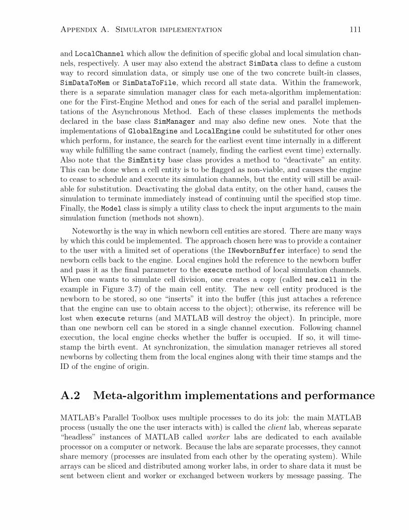
Appendix A. Simulator implementation 111
and LocalChannel which allow the definition of specific global and local simulation chan-nels, respectively. A user may also extend the abstract SimData class to define a customway to record simulation data, or simply use one of the two concrete built-in classes,SimDataToMem or SimDataToFile, which record all state data. Within the framework,there is a separate simulation manager class for each meta-algorithm implementation:one for the First-Engine Method and ones for each of the serial and parallel implemen-tations of the Asynchronous Method. Each of these classes implements the methodsdeclared in the base class SimManager and may also define new ones. Note that theimplementations of GlobalEngine and LocalEngine could be substituted for other oneswhich perform, for instance, the search for the earliest event time internally in a differentway while fulfilling the same contract (namely, finding the earliest event time) externally.Also note that the SimEntity base class provides a method to “deactivate” an entity.This can be done when a cell entity is to be flagged as non-viable, and causes the engineto cease to schedule and execute its simulation channels, but the entity will still be avail-able for substitution. Deactivating the global data entity, on the other hand, causes thesimulation to terminate immediately instead of continuing until the specified stop time.Finally, the Model class is simply a utility class to check the input arguments to the mainsimulation function (methods not shown).
Noteworthy is the way in which newborn cell entities are stored. There are many waysby which this could be implemented. The approach chosen here was to provide a containerto the user with a limited set of operations (the INewbornBuffer interface) to send thenewborn cells back to the engine. Local engines hold the reference to the newborn bufferand pass it as the final parameter to the execute method of local simulation channels.When one wants to simulate cell division, one creates a copy (called new cell in theexample in Figure 3.7) of the main cell entity. The new cell entity produced is thenewborn to be stored, so one “inserts” it into the buffer (this just attaches a referencethat the engine can use to obtain access to the object); otherwise, its reference will belost when execute returns (and MATLAB will destroy the object). In principle, morethan one newborn cell can be stored in a single channel execution. Following channelexecution, the local engine checks whether the buffer is occupied. If so, it will time-stamp the birth event. At synchronization, the simulation manager retrieves all storednewborns by collecting them from the local engines along with their time stamps and theID of the engine of origin.
A.2 Meta-algorithm implementations and performance
MATLAB’s Parallel Toolbox uses multiple processes to do its job: the main MATLABprocess (usually the one the user interacts with) is called the client lab, whereas separate“headless” instances of MATLAB called worker labs are dedicated to each availableprocessor on a computer or network. Because the labs are separate processes, they cannotshare memory (processes are insulated from each other by the operating system). Whilearrays can be sliced and distributed among worker labs, in order to share data it must besent between client and worker or exchanged between workers by message passing. The

Appendix A. Simulator implementation 112
Asynchronous Method managers support three different modes of execution, one in afully sequential manner which does not make use of the parallel toolbox (serial mode, inwhich everything takes place on the client lab), and two parallel modes which make useof different language constructs from the toolbox. These are called parfor mode, in whichthe meta-algorithm uses MATLAB’s parfor loop construct for releasing the local engines;and spmd mode, in which the meta-algorithm is implemented using a construct calledsingle-program-multiple-data (spmd) blocks. Spmd blocks can use a special data type tocreate, gather, and reference variables on the worker labs directly. In spmd mode, suchblocks need to be incorporated into a global simulation channel if it needs to access a cellentity object, because the cell entities always reside on worker labs. In parfor mode, onthe other hand, one never includes parallel logic in simulation channel code, but parforexecution may involve a higher communication overhead.
Note that the time complexity of the simulation meta-algorithms depend strongly onthe way the searches for earliest event times are implemented, as well as model-specificdetails such as the number of engines N versus the number of channels in each engine M .The current First-Engine Method implementation holds an array of the engine next eventtimes and uses the built-in min function to find the smallest element. This approach haslinear or O(N) time complexity, where N is the number of engines. As a result, the First-Engine implementation tends to run more slowly than the serial Asynchronous Methodimplementation on the same model because the latter only performs O(M) searches andM is usually much smaller than N . However, for large N or M , using a data structuresuch as a binary heap to create an indexed priority queue (as prescribed in the Next-Reaction variant of the SSA) would lead to overall more efficient O(1) complexity forobtaining the smallest element and logarithmic complexity for sorting the event timeseach time one is updated. Such data structures are not supported natively in MATLAB.
Also, note that a protocol must be specified for handling simultaneous events. First, iftwo simulation channels in the same engine are scheduled to occur at the same time, theorder in which the channels were provided to the program determines the priority orderfor firing. Second, if a global channel and a local channel are scheduled to fire at the sametime, the local channel gets executed first. Lastly, because the simulation events executedby different local simulation engines do not influence one another, it does not matter inwhat order they are executed, so no protocol needs to be enforced. In the AsynchronousMethod, they may be executed concurrently, while in the First-Engine method the orderwould be determined by the kind of data structure being used internally to sort the listof next event times of the engines.
Unfortunately, in developing their new class system, The MathWorks decided on adeterministic method for automatic memory management of objects that persist beyondthe scope of function calls (i.e., handle objects) [113]. The details are undocumented,but involves doing bookkeeping in the background whenever functions or methods re-turn. It also creates very long latencies when passing arrays of handle objects betweenlabs. This, among other factors, ultimately proved to be unacceptably costly in termsof scale-up performance. Because these performance bottlenecks were not representativeof the true run-time complexity of the framework algorithms, no run-time performance

Appendix A. Simulator implementation 113
benchmarks were performed using the MATLAB implementation. However, a C++ im-plementation, currently in final stages of development, demonstrates drastically moreefficient and very practical run-times (e.g., 1-2min for each the 10,000-cell simulations inSection 4.4 running serially vs ∼2h30min in MATLAB running in parallel on an 8-coreLinux desktop!).

Appendix B
The birth-migration process
It will be shown here that the bistable switching model described in Section 4.2 is equiv-alent to a birth-migration continuous-time Markov chain, and expressions for the firstmoments of the variables of interest will be derived.
In the bistable switching model, each individual in one state can switch to the op-posing state. The occurrence of a switching event in non-overlapping time intervals isindependent (the process is memoryless), and the probability of an event or “arrival” inan infinitesimal interval is
Pr{switch event in (t, t+ dt)} = kidt (B.1)
This is also called a (homogeneous) Poisson process with rate ki.
Recall that in addition to switching, each individual is also subject to a birth process.This can be formulated as the simultaneous occurrence of three independent events: theremoval of one individual from the i-subpopulation (rate λi) and the addition of two newindividuals with state chosen according to probability σi. For instance, supposing anOFF-cell gives birth, there are three mutually exclusive possible outcomes:
1. Both cells are born in the OFF-state (a cis birth)
2. One cell is born in each state (a split birth)
3. Both cells are born in the ON-state (a trans birth)
By independence, this translates into the following probabilistic rate equations
Pr{cis birth in (t, t+ dt)} = σ2i λi, (B.2)
Pr{split birth in (t, t+ dt)} = σi(1− σi)λi, (B.3)
Pr{trans birth in (t, t+ dt)} = (1− σi)2λi, (B.4)
which are all memoryless and have constant rates; hence, they are all homogeneousPoisson processes.
114

Appendix B. The birth-migration process 115
It is a fact that the inter-arrival times of a Poisson process are exponentially dis-tributed. That is, for a Poisson process with rate µ, the waiting time T to the nextarrival obeys
Pr{T = τ}dτ = −µe−µτdτ. (B.5)
We will make use the following property of the exponential distribution:
Lemma 1. Suppose that Y1, Y2, . . . , Yn are independent exponential random variableswith Yi having rate µi, i = 1, . . . , n. Then the first order statistic min(Y1, . . . , Yn) is also
exponentially distributed with raten∑i=1
µi.
For a proof of this result, see [114], p.291.
Let the random variables X0(t) and X1(t) represent the number of cells in the OFFand ON states, respectively. Then Lemma 1 tells us that given the system is in stateX0 = x0 and X1 = x1 at time t, if we superimpose together all the 0 → 1 switchingprocesses for all cells in the OFF-state, the occurrence of the first of the 0→ 1 switchingevents (i.e., the shortest waiting time) is also exponentially distributed, with rate x0k1.Similarly the first 1 → 0 switching event would obey rate x1k0, the first cis birth eventamong ON-cells would obey rate x1σ
21λ1, and so on. These events represent the transitions
of the subpopulation counts (x0, x1) between states. This can be illustrating using a statetransition diagram for the subpopulation counts:
[x0x1
]
[x0x1
]+
[01
] [x0x1
]+
[10
] [x0x1
]+
[−12
]
[x0x1
]+
[1−1
] [x0x1
]+
[−11
]
[x0x1
]+
[10
] [x0x1
]+
[01
] [x0x1
]+
[2−1
]
0-split 0-cis 0-trans
1-split 1-cis 1-trans
switch OFF switch ON
σ0(1− σ0)λ0x0 σ20λ0x0 (1− σ0)2λ0x0
σ1(1− σ1)λ1x1 σ21λ1x1
(1− σ1)2λ1x1
k0x1 k1x0
The resulting system is a BM process. Because all the transitions are Markovian(have exponentially distributed waiting times in isolation), the system is a continuous-time Markov chain, like a chemical reaction model. Its probability distribution thereforeobeys a master equation. We will use here the notation used for chemical master equations
∂P (x, t)
∂t=
8∑j=1
[aj(x− νj)P (x− νj , t)− aj(x)P (x, t)] , (B.6)

Appendix B. The birth-migration process 116
which sums over all 8 transitions both into and out of the state x = [x0, x1]T , with
“propensities” or transition rates aj(x), and “stoichiometries” νj as shown in the dia-gram, j = 1, . . . , 8. Multiplying equation B.6 through by x and summing over all x gives
d〈X(t)〉dt
=8∑j=1
νj 〈aj(X(t)〉 . (B.7)
In general, for nonlinear systems one cannot infer much about average behaviour, butfortunately, all the transition rates in the BM process are linear in the variables x0 andx1, giving
d〈X(t)〉dt
=8∑j=1
νjaj(〈X(t)〉) , (B.8)
which is a closed ODE solution for the first moment 〈X(t)〉 . Accordingly, the result forthis system is equation 4.10.
However, we are not directly interested in the absolute subpopulation counts, butrather their relative sizes. Let Fi(t) = Xi(t)/Xtotal(t), where Xtotal = X0 +X1, then
〈Fi〉 =
⟨Xi(t)
X0(t) +X1(t)
⟩, i = 0, 1, (B.9)
and also〈F0(t)〉+ 〈F1(t)〉 = 1. (B.10)
Note that if Xtotal is sufficiently large that fluctuations are small, then fluctuations in1/Xtotal are vanishingly small. This means that
Cov
(Xi,
1
Xtotal
)→ 0, i = 0, 1, (B.11)
allowing the angle bracket in equation B.9 to be broken up
〈Fi〉 ≈〈Xi〉
〈X0 +X1〉=
〈Xi〉〈X0〉 + 〈X1〉
, i = 0, 1. (B.12)
With equation B.12, a closed-form expression can be obtained for the first momentsfrom equations 4.10 using the quotient rule of differentiation
〈F0(t)〉 = 1− 〈F1(t)〉 ,
d 〈F1(t)〉dt
= (λ0 − λ1) 〈F1(t)〉2 + [λ0(2σ0 − 3) + λ1(2σ1 − 1)− k0 − k1] 〈F1(t)〉
+ k1 − 2λ0(σ0 − 1),
which are exactly equations 4.12 and 4.13. They can be solved by numerical integration.

Appendix B. The birth-migration process 117
Alternatively, note that equation 4.13 is of a special form
df
dt= Af 2 +Bf + C, (B.13)
called a Riccati differential equation, which has an analytical solution.