a framework for performing forensic and investigatory ... · pdf filea framework for...
TRANSCRIPT
A FRAMEWORK FOR PERFORMING FORENSIC AND INVESTIGATORY
SPEAKER COMPARISONS USING AUTOMATED METHODS
by
DAVID BRIAN MARKS
B.S., Oklahoma State University, 1984
M.S., Oklahoma State University, 1985
A thesis submitted to the
Faculty of the Graduate School of the
University of Colorado in partial fulfillment
of the requirement for the degree of
Master of Science
Recording Arts Program
2017

ii
© 2017
DAVID BRIAN MARKS
ALL RIGHTS RESERVED

iii
This thesis for the Master of Science degree by
David Brian Marks
has been approved for the
Recording Arts Program
by
Catalin Grigoras, Chair
Jeff Smith
Lorne Bregitzer
Date: May 13, 2017

iv
Marks, David Brian (M.S., Recording Arts Program)
A Framework for Performing Forensic and Investigatory Speaker Comparisons Using
Automated Methods
Thesis directed by Associate Professor Catalin Grigoras
ABSTRACT
Recent innovations in the algorithms and methods employed for forensic
speaker comparisons of voice recordings have resulted in automated tools that greatly
simplify the analysis process. With the continual advances in computational capacity, it
is all too easy to simply click a few buttons to initiate an analysis that yields an
automated result. However, the underlying capability of the technology, while
impressive under favorable conditions, remains relatively fragile if the tools are used
beyond their designed capabilities. Their performance can be compromised further by
the inherent nature of speech. As with other common forensic disciplines such as DNA
analysis or fingerprint comparison, the evidence under analysis contains qualities that
can be correlated to an individual speaker. Unlike many disciplines, however, the
evidence also reflects the underlying behavior of the speaker and contains additional
variability due to the words spoken, the speaking style, the emotional state and health
of the speaker, the transmission channel, the recording technology and conditions, and
other crucial factors. In any forensic discipline, the analysis process must be based on
established scientific principles, follow accepted practices, and operate within an
accepted forensic framework to render reliable and supportable conclusions to a trier
of fact. For judicial applications, conclusions must be able to withstand the adversarial
scrutiny of the legal system. For investigative applications, forensic results may not be

v
required to withstand the same level of scrutiny, but ethical obligations nevertheless
impart an equal responsibility to an examiner to deliver accurate and unbiased results.
Unfortunately, in the forensic speaker comparison community, no formal standards
have gained universal acceptance (although individual laboratories will have their own
standard operating procedures if they are operating in a responsible manner). To this
end, this document proposes a framework for conducting forensic speaker comparisons
that encompasses case setup, evidence handling, data preparation, technology
assessment and applicability, guidelines for analysis, drawing conclusions, and
communicating results.
The form and content of this abstract are approved. I recommend its publication.
Approved: Catalin Grigoras

vi
DEDICATION
I would like to dedicate this thesis to my wife, Melinda, whose love, patience, and
support made this possible. I also would like to dedicate this thesis to my children,
Stephanie and Jared, who always were motivation for me to want to do better and be
better.
vii
ACKNOWLEDGEMENTS
I would like to express my gratitude to my thesis advisor, Dr. Catalin Grigoras,
for his continued enthusiasm and support in my study of forensics, and to Jeff Smith for
his support and friendship. I also am grateful to my other instructors and to my fellow
students for their patience with my incessant questions during classroom sessions. My
special thanks go to Leah Haloin who excelled at keeping me on track throughout the
program to meet the required milestones.
I particularly would like to thank my colleagues on the Speaker Recognition
subcommittee of the Organization of Scientific Area Committees (OSAC-SR) for their
enthusiastic collaboration and for providing a sounding board (and often a sanity
check) for my ideas. We stand on the shoulders of giants. Specifically, I am grateful to
Dr. Hirotaka Nakasone of the FBI Forensic Audio Video and Image Analysis Unit
(FAVIAU), Dr. Douglas Reynolds and Dr. Joseph Campbell of MIT Lincoln Laboratory,
Ms. Reva Schwartz of the National Institute of Standards and Technology (NIST), and
Stephen, for their continued support and friendship.
viii
TABLE OF CONTENTS
CHAPTER
I. INTRODUCTION ..................................................................................................................................... 1
Terminology ............................................................................................................................................ 3
Challenges of Voice Forensics .......................................................................................................... 4
Scope .......................................................................................................................................................... 5
II. BACKGROUND ........................................................................................................................................ 7
Scientific Foundations ......................................................................................................................... 7
The Scientific Method .................................................................................................................. 8
Bias Effects ...................................................................................................................................... 9
Legal Foundations .............................................................................................................................. 19
Rules of Evidence ....................................................................................................................... 19
Federal Case Law ....................................................................................................................... 22
State Case Law ............................................................................................................................ 24
Factors in Speaker Recognition .................................................................................................... 25
The Nature of the Human Voice ........................................................................................... 26
Speaker Recognition Systems ............................................................................................... 27
Bias Effects ................................................................................................................................... 40
Standards ...................................................................................................................................... 41
Historical Baggage ..................................................................................................................... 41

ix
III. COMPARISON FRAMEWORK ......................................................................................................... 43
Case Assessment................................................................................................................................. 44
Forensic Request ........................................................................................................................ 45
Administrative Assessment ................................................................................................... 46
Technical Assessment .............................................................................................................. 49
Decision to Proceed with Analysis ...................................................................................... 53
Analysis and Processing .................................................................................................................. 55
Data Preparation ........................................................................................................................ 56
Data Enhancement .................................................................................................................... 57
Selection of the Relevant Population ................................................................................. 58
System Performance and Calibration ................................................................................ 59
Combining Results from Multiple Methods or Systems.............................................. 61
Conclusions .......................................................................................................................................... 64
Interpreting Results .................................................................................................................. 64
Communicating Results ........................................................................................................... 67
Case Studies .......................................................................................................................................... 68
Case Study 1 ................................................................................................................................. 70
Case Study 2 ................................................................................................................................. 87
Case Study 3 ............................................................................................................................... 102
Case Study 4 ............................................................................................................................... 125

x
Case Study Summary .............................................................................................................. 142
IV. SUMMARY AND CONCLUSIONS .................................................................................................. 144
Challenges in the Relevant Population .................................................................................... 146
Fusion for Multiple Algorithms .................................................................................................. 147
Verbal Scale Standards for Reporting Results ...................................................................... 147
Data and Standards for Validation ............................................................................................ 148
REFERENCES .............................................................................................................................................. 149
INDEX ............................................................................................................................................................ 155

xi
LIST OF TABLES
TABLE
1. Terms used in this document. ............................................................................................................. 4
2. Potential Mismatch Conditions ........................................................................................................ 26
3. Verbal scale adapted from ENFSI guidelines for forensic reporting. ................................ 66
4. Verbal scale for corroboration measure and fusion. ............................................................... 66
5. Case 1 evidence files. ........................................................................................................................... 70
6. Case 1 Q1 assessment. ......................................................................................................................... 71
7. Case 1 K1 assessment. ......................................................................................................................... 72
8. Case 1 fusion results. ........................................................................................................................... 87
9. Case 2 evidence files. ........................................................................................................................... 88
10. Case 2 Q1 assessment. ...................................................................................................................... 89
11. Case 2 K1 assessment. ...................................................................................................................... 89
12. Case 2 fusion results. ....................................................................................................................... 102
13. Case 3 evidence files. ....................................................................................................................... 103
14. Case 3 Q1 assessment. .................................................................................................................... 104
15. Case 3 K1 assessment. .................................................................................................................... 105
16. Case 3 fusion results. ....................................................................................................................... 124
17. Case 3 fusion results using Tamil relevant population. ..................................................... 124
18. Case 4 evidence files. ....................................................................................................................... 125
19. Case 4 Q1 assessment. .................................................................................................................... 127
20. Case 4 K1 assessment. .................................................................................................................... 127
21. Case 4 K2 assessment. .................................................................................................................... 128

xii
22. Case 4 fusion results for Q1 vs. K1. ............................................................................................ 141
23. Case 4 fusion results for Q1 vs. K2. ............................................................................................ 141

xiii
LIST OF FIGURES
FIGURE
1. Map of states using Frye vs. Daubert. ............................................................................................ 25
2. Process flow for a typical speaker recognition system. ......................................................... 27
3. Simulated scores for a system with good discrimination...................................................... 31
4. DET plot for a simulated system with good discrimination. ................................................ 32
5. Simulated scores for a system with less discrimination. ....................................................... 33
6. DET plot for a simulated system with less discrimination. .................................................. 34
7. Simulated scores for a system with good discrimination on a smaller data set. .......... 35
8. DET plot for a simulated system with good discrimination on a small data set. ......... 35
9. Simulated scores for a system with a multimodal non-target distribution. .................. 36
10. DET plot for a simulated system with a multimodal non-target distribution. ........... 37
11. Simulated scores for a system with triangular distributions. ........................................... 38
12. DET plot for a simulated system with triangular score distributions. .......................... 38
13. Framework flowchart for forensic speaker comparison. ................................................... 44
14. System with good discrimination overlaid with corroboration function. .................... 63
15. Case 1 (1v2) score distribution with GMM-UBM algorithm. ............................................. 75
16. Case 1 (1v2) DET plot with GMM-UBM algorithm. ................................................................ 75
17. Case 1 (2v1) score distribution with GMM-UBM algorithm. ............................................. 76
18. Case 1 (2v1) DET plot with GMM-UBM algorithm. ................................................................ 76
19. Case 1 (1v2 and 2v1) score ranking with GMM-UBM algorithm. .................................... 77
20. Case 1 (1v2) score distribution with SVM algorithm. .......................................................... 78
21. Case 1 (1v2) DET plot with SVM algorithm. ............................................................................. 78

xiv
22. Case 1 (2v1) score distribution with SVM algorithm. .......................................................... 79
23. Case 1 (2v1) DET plot with SVM algorithm. ............................................................................. 79
24. Case 1 (1v2 and 2v1) score ranking with SVM algorithm. ................................................. 80
25. Case 1 (1v2) score distribution with i-Vector algorithm. ................................................... 81
26. Case 1 (1v2) DET plot with i-Vector algorithm. ..................................................................... 81
27. Case 1 (2v1) score distribution with i-Vector algorithm. ................................................... 82
28. Case 1 (2v1) DET plot with i-Vector algorithm. ..................................................................... 82
29. Case 1 (1v2 and 2v1) score ranking with i-Vector algorithm. .......................................... 83
30. Case 1 (1v2) score distribution with DNN algorithm. .......................................................... 84
31. Case 1 (1v2) DET plot with DNN algorithm. ............................................................................ 84
32. Case 1 (2v1) score distribution with DNN algorithm. .......................................................... 85
33. Case 1 (2v1) DET plot with DNN algorithm. ............................................................................ 85
34. Case 1 (1v2 and 2v1) score ranking with DNN algorithm. ................................................. 86
35. Case 2 (1v2) score distribution with GMM-UBM algorithm. ............................................. 92
36. Case 2 (1v2) DET plot with GMM-UBM algorithm. ................................................................ 92
37. Case 2 (2v1) score distribution with GMM-UBM algorithm. ............................................. 93
38. Case 2 (2v1) DET plot with GMM-UBM algorithm. ................................................................ 93
39. Case 2 (1v2 and 2v1) score ranking with GMM-UBM algorithm. .................................... 94
40. Case 2 (1v2) score distribution with SVM algorithm. .......................................................... 95
41. Case 2 (1v2) DET plot with SVM algorithm. ............................................................................. 95
42. Case 2 (2v1) score distribution with SVM algorithm. .......................................................... 96
43. Case 2 (2v1) DET plot with SVM algorithm. ............................................................................. 96
44. Case 2 (1v2 and 2v1) score ranking with SVM algorithm. ................................................. 97
xv
45. Case 2 (1v2 or 2v1) score distribution with i-Vector algorithm. ..................................... 98
46. Case 2 (1v2 or 2v1) DET plot with i-Vector algorithm. ....................................................... 98
47. Case 2 (1v2 and 2v1) score ranking with i-Vector algorithm. .......................................... 99
48. Case 2 (1v2 or 2v1) score distribution with DNN algorithm. ......................................... 100
49. Case 2 (1v2 or 2v1) DET plot with DNN algorithm. ............................................................ 100
50. Case 2 (1v2 and 2v1) score ranking with DNN algorithm. ............................................... 101
51. Case 3 (1v2) score distribution with GMM-UBM algorithm. ........................................... 108
52. Case 3 (1v2) DET plot with GMM-UBM algorithm. .............................................................. 108
53. Case 3 (2v1) score distribution with GMM-UBM algorithm. ........................................... 109
54. Case 3 (2v1) DET plot with GMM-UBM algorithm. .............................................................. 109
55. Case 3 (1v2 and 2v1) score ranking with GMM-UBM algorithm. .................................. 110
56. Case 3 (1v2) score distribution with SVM algorithm. ........................................................ 111
57. Case 3 (1v2) DET plot with SVM algorithm. ........................................................................... 111
58. Case 3 (2v1) score distribution with SVM algorithm. ........................................................ 112
59. Case 3 (2v1) DET plot with SVM algorithm. ........................................................................... 112
60. Case 3 (1v2 and 2v1) score ranking with SVM algorithm. ............................................... 113
61. Case 3 (1v2 or 2v1) score distribution with i-Vector algorithm. ................................... 114
62. Case 3 (1v2 or 2v1) DET plot with i-Vector algorithm. ..................................................... 114
63. Case 3 (1v2 and 2v1) score ranking with i-Vector algorithm. ........................................ 115
64. Case 3 (1v2 or 2v1) score distribution with DNN algorithm. ......................................... 116
65. Case 3 (1v2 or 2v1) DET plot with DNN algorithm. ............................................................ 116
66. Case 3 (1v2 and 2v1) score ranking with DNN algorithm. ............................................... 117
67. Case 3 (1v2) with GMM-UBM algorithm using Tamil relevant population................ 118
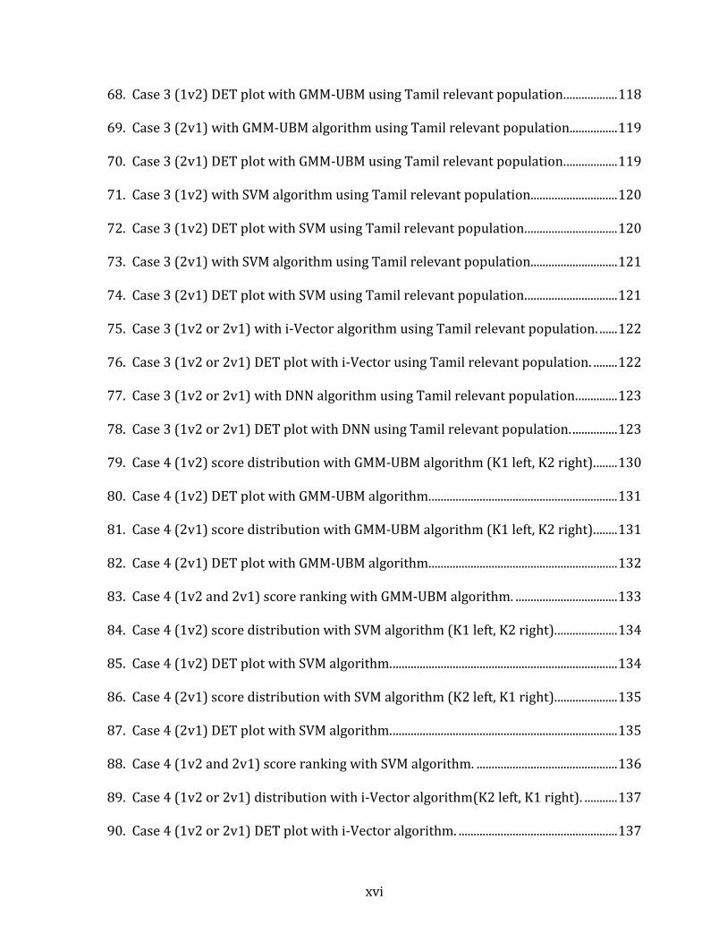
xvi
68. Case 3 (1v2) DET plot with GMM-UBM using Tamil relevant population. ................. 118
69. Case 3 (2v1) with GMM-UBM algorithm using Tamil relevant population................ 119
70. Case 3 (2v1) DET plot with GMM-UBM using Tamil relevant population. ................. 119
71. Case 3 (1v2) with SVM algorithm using Tamil relevant population............................. 120
72. Case 3 (1v2) DET plot with SVM using Tamil relevant population. .............................. 120
73. Case 3 (2v1) with SVM algorithm using Tamil relevant population............................. 121
74. Case 3 (2v1) DET plot with SVM using Tamil relevant population. .............................. 121
75. Case 3 (1v2 or 2v1) with i-Vector algorithm using Tamil relevant population. ...... 122
76. Case 3 (1v2 or 2v1) DET plot with i-Vector using Tamil relevant population. ........ 122
77. Case 3 (1v2 or 2v1) with DNN algorithm using Tamil relevant population. ............. 123
78. Case 3 (1v2 or 2v1) DET plot with DNN using Tamil relevant population. ............... 123
79. Case 4 (1v2) score distribution with GMM-UBM algorithm (K1 left, K2 right). ....... 130
80. Case 4 (1v2) DET plot with GMM-UBM algorithm. .............................................................. 131
81. Case 4 (2v1) score distribution with GMM-UBM algorithm (K1 left, K2 right). ....... 131
82. Case 4 (2v1) DET plot with GMM-UBM algorithm. .............................................................. 132
83. Case 4 (1v2 and 2v1) score ranking with GMM-UBM algorithm. .................................. 133
84. Case 4 (1v2) score distribution with SVM algorithm (K1 left, K2 right). .................... 134
85. Case 4 (1v2) DET plot with SVM algorithm. ........................................................................... 134
86. Case 4 (2v1) score distribution with SVM algorithm (K2 left, K1 right). .................... 135
87. Case 4 (2v1) DET plot with SVM algorithm. ........................................................................... 135
88. Case 4 (1v2 and 2v1) score ranking with SVM algorithm. ............................................... 136
89. Case 4 (1v2 or 2v1) distribution with i-Vector algorithm(K2 left, K1 right). ........... 137
90. Case 4 (1v2 or 2v1) DET plot with i-Vector algorithm. ..................................................... 137

xvii
91. Case 4 (1v2 and 2v1) score ranking with i-Vector algorithm. ........................................ 138
92. Case 4 (1v2 or 2v1) score distribution with DNN algorithm(K2 left, K1 right). ...... 139
93. Case 4 (1v2 or 2v1) DET plot with DNN algorithm. ............................................................ 139
94. Case 4 (1v2 and 2v1) score ranking with DNN algorithm. ............................................... 140

xviii
ABBREVIATIONS AND DEFINITIONS
DET plot Detection Error Tradeoff plot that shows the performance of a binary classification system by plotting false rejection rate vs. false acceptance rate
EER Equal Error Rate ENFSI European Network of Forensic Science Institutes FAVIAU FBI Forensic Audio, Video, and Image Analysis Unit FBI Federal Bureau of Investigation FSC Forensic Speaker Comparison GMM-UBM Gaussian Mixture Model – Universal Background Model ISC Investigatory Speaker Comparison NAS National Academy of Sciences NIST National Institute of Standards and Technology OSAC Organization of Scientific Area Committees OSAC-SR Speaker Recognition subcommittee in the OSAC hierarchy PCAST President’s Council of Advisors on Science and Technology PLDA Probabilistic Linear Discriminant Analysis SNR Signal-to-noise ratio SPQA Speech Quality Assurance package from NIST SRE Speaker Recognition Evaluation, a competition run by NIST to allow
researchers to compare algorithm performance on standard data sets SVM Support Vector Machine SWG Scientific Working Group SWGDE Scientific Working Group for Digital Evidence V&V Validation and Verification
1
CHAPTER I
INTRODUCTION
In 2009, the National Research Council of the National Academy of Sciences
(NAS) published a report, Strengthening Forensic Science in the United States: A Path
Forward [1]. The report was highly critical of the state of forensic science:
The forensic science system, encompassing both research and practice, has serious problems that can only be addressed by a national commitment to overhaul the current structure that supports the forensic science community in this country. This can only be done with effective leadership at the highest levels of both federal and state governments, pursuant to national standards, and with a significant infusion of federal funds.
The recommendations issued in the report included such reforms as improving
the scientific basis of forensic disciplines, promoting reliable and consistent analysis
methodologies, standardizing terminology and reporting conventions, and requiring
validation and verification of forensic methods and practices.
In 2016, a report from the President’s Council of Advisors on Science and
Technology (PCAST) [2] concluded that there are two important gaps in the science that
should be addressed to ensure the “foundational validity” of forensic evidence:
1. the need for clarity about the scientific standards for the validity and
reliability of forensic methods, and
2. the need to evaluate specific forensic methods to determine whether they
have been scientifically established to be valid and reliable.
The discipline of forensic speaker comparison (FSC), while not new, has seen
recent innovations in the algorithms and methods used, resulting in automated tools
that greatly simplify the analysis process. With the continual advances in

2
computational capacity, it is all too easy to simply click a few buttons to initiate an
analysis that yields an automated result. The technology can be easy to use, but it also
can be easy to misuse, either intentionally by unscrupulous practitioners or
unintentionally by naïve but well-meaning practitioners. Additionally, the results
produced by the tools can easily be misunderstood or misinterpreted if the analysis is
not structured or conducted appropriately.
The current capability of the underlying technology, while impressive under
favorable conditions, remains relatively fragile if the tools are used beyond their
designed capabilities. Their performance can be compromised further by the inherent
nature of speech. As with other common forensic disciplines such as DNA analysis or
fingerprint comparison, the evidence under analysis contains qualities that can be
correlated to an individual speaker. Unlike many disciplines, however, the evidence
also reflects the underlying behavior of the speaker and contains additional variability
due to the words spoken, the speaking style and state of the speaker, the transmission
channel, the recording technology and conditions, and other crucial factors.
In any forensic discipline, fundamental ethical obligations require that the
analysis process be based on established scientific principles, follow accepted practices,
and operate within a forensically sound framework to render reliable and supportable
conclusions to a trier of fact. Examiners must strive to deliver objective, unbiased, and
accurate results where people’s lives may be at stake. Additionally for judicial
applications, conclusions must be able to withstand the adversarial scrutiny of the legal
system. For investigative applications, forensic results may not be required to
withstand the same level of scrutiny, but the same ethical obligations nevertheless

3
impart an equal responsibility to examiners with respect to the rigor with which they
conduct their analyses.
Unfortunately, in the forensic speaker comparison community, no formal
standards have gained universal acceptance, although individual laboratories will have
their own standard operating procedures if they are operating in a responsible manner.
To this end (and in light of the NAS report), this document proposes a framework for
conducting forensic speaker comparisons that encompasses case setup, evidence
handling, data preparation, technology assessment and applicability, guidelines for
analysis, drawing conclusions, and communicating results. It also points out areas in
which the limits of the technology restrict the application of scientific rigor to the
overall process in the hope that these areas can be addressed by ongoing research.
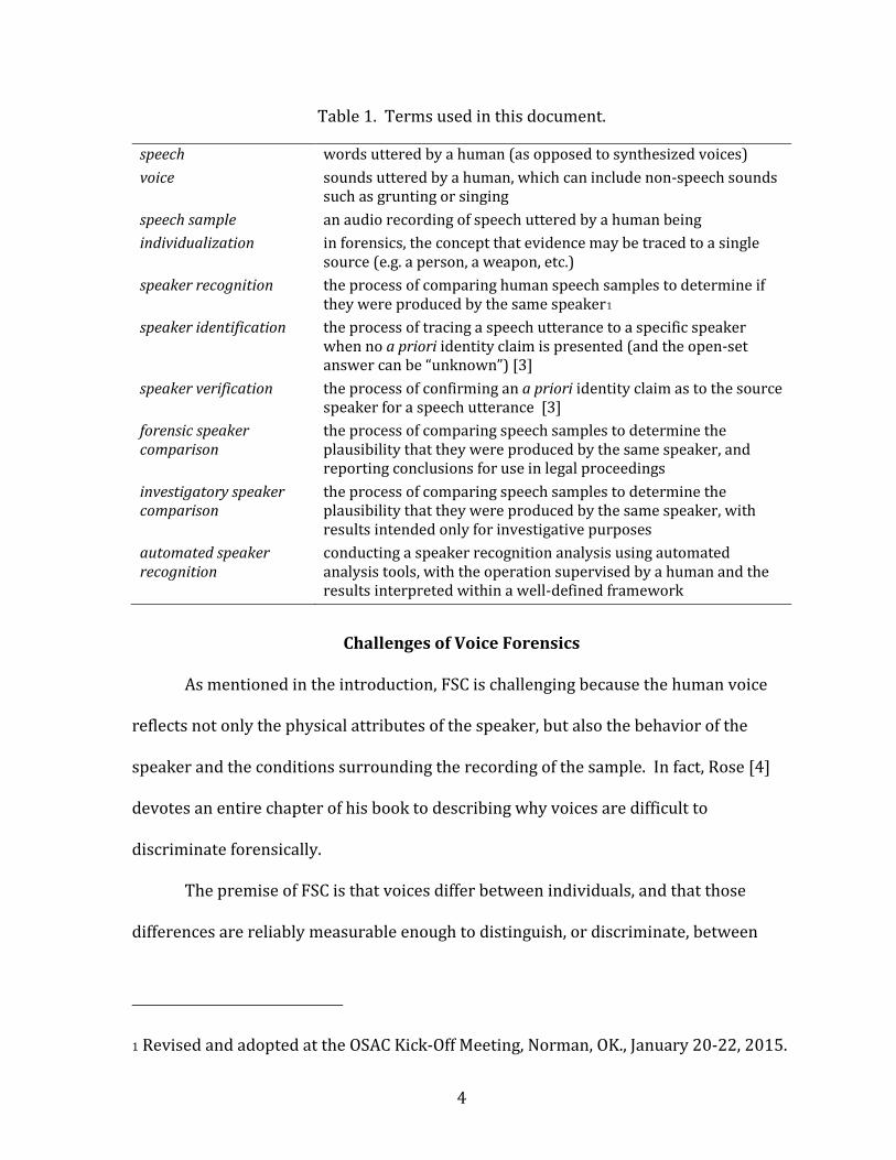
Terminology
In general, the terminology used in speaker recognition is agreed upon, but no
official standard has yet emerged. For example, the terms “speaker recognition”,
“speaker identification”, “speaker verification”, and “voice recognition” are sometimes
confused, and often used interchangeably. Similarly, practitioners with different
backgrounds and training often use “voice” and “speech” differently. For the purposes
of this document, the definitions in Table 1 will be used.
This document focuses on conducting forensic speaker comparisons (FSCs) using
automated speaker recognition (or more accurately, human-supervised automatic
speaker recognition), but the position of this paper is that investigatory speaker
comparisons (ISCs) should be conducted with the same degree of scientific rigor.
4
Table 1. Terms used in this document.
speech words uttered by a human (as opposed to synthesized voices) voice sounds uttered by a human, which can include non-speech sounds
such as grunting or singing speech sample an audio recording of speech uttered by a human being individualization in forensics, the concept that evidence may be traced to a single
source (e.g. a person, a weapon, etc.) speaker recognition the process of comparing human speech samples to determine if
they were produced by the same speaker1 speaker identification the process of tracing a speech utterance to a specific speaker
when no a priori identity claim is presented (and the open-set answer can be “unknown”) [3]
speaker verification the process of confirming an a priori identity claim as to the source speaker for a speech utterance [3]
forensic speaker comparison
the process of comparing speech samples to determine the plausibility that they were produced by the same speaker, and reporting conclusions for use in legal proceedings
investigatory speaker comparison
the process of comparing speech samples to determine the plausibility that they were produced by the same speaker, with results intended only for investigative purposes
automated speaker recognition
conducting a speaker recognition analysis using automated analysis tools, with the operation supervised by a human and the results interpreted within a well-defined framework
Challenges of Voice Forensics
As mentioned in the introduction, FSC is challenging because the human voice
reflects not only the physical attributes of the speaker, but also the behavior of the
speaker and the conditions surrounding the recording of the sample. In fact, Rose [4]
devotes an entire chapter of his book to describing why voices are difficult to
discriminate forensically.
The premise of FSC is that voices differ between individuals, and that those
differences are reliably measurable enough to distinguish, or discriminate, between
1 Revised and adopted at the OSAC Kick-Off Meeting, Norman, OK., January 20-22, 2015.

5
those individuals. The goal of FSC, then, is to analyze this between-speaker (or inter-
speaker) variation to recognize a particular speaker. Unfortunately, complications arise
because an individual also has within-speaker (or intra-speaker) variation due to the
words spoken, the emotions in play (excitement, anger, sadness, etc.), the speaker’s
health, the speaking style (reading, conversational, shouting, etc.), and the situation
(sitting quietly, running, etc.). Additional complications arise because of differences in
the recording conditions of the samples being compared (background noise,
microphone type, etc.). That is, there are channel variations between the recordings.
Much of the ongoing research in speaker recognition attempts to develop algorithms
with increased sensitivity to between-speaker variations while decreasing sensitivity to
all other variations.
Scope
While this document proposes a framework for conducting forensic speaker
comparisons, it does not attempt to provide thorough coverage of procedures that
would be specific to individual laboratories or of practices that are well covered by
published documents. However, where appropriate, considerations unique to FSC will
be included and references provided to relevant documents that are more general in
nature. For example, different labs will almost certainly handle examiner notes and
case review practices differently. As a more technical example, some best practice
documents for audio processing recommend methods that enhance audio for human
listening, but such methods may degrade the performance of speaker recognition tools.
Since the tools discussed in this document are based on computer algorithms,
the assumption is that all audio recordings are in a digital format, and that any analog

6
recordings will be converted to digital using established practices [5]. The Scientific
Working Group on Digital Evidence (SWGDE) group and the Digital Evidence
subcommittee within the Organization of Scientific Area Committees (OSAC-DE)
provide excellent resources in this area. Also, analysis for assessing the authenticity of
recordings is covered elsewhere [6] [7], so the assumption in this document is that the
evidence recordings have already been authenticated if required by the case at hand.
7
CHAPTER II
BACKGROUND
The NAS report was critical of the science (or lack thereof) that provides the
foundation for the forensic science community. Ultimately, the results of the science
reach a decision maker, and without a strong foundation, the decision maker cannot
make sound decisions. In forensic applications, the decision maker usually is the trier of
fact (i.e. the judge and/or jury), but alternatively could be a district attorney that
decides whether the strength of evidence warrants taking a case to trial or settling out of
court. For investigatory applications in which the evidence is merely being used to
pursue an investigation that is not expected to lead to a courtroom (e.g. law
enforcement, intelligence, or private investigations), the decision maker typically is the
lead investigator. Regardless the application, ethical obligations require forensic
professionals to conduct examinations with all appropriate rigor as if the results were
to be presented in court. The following sections discuss the basic principles involved.
Scientific Foundations
If having a rigorous scientific basis is a requirement for forensic applications and
the NAS report asserts that the current forensic science system not actually based on
science and is too subjective [8], then Occam’s Razor [9] would suggest that, in general,
the forensic community believed that scientific principles were being followed. To be a
bit more precise, the forensic community was biased by its own belief in the validity of
its scientific concepts and practices. Since according to the NAS report this belief
apparently is not true, then how indeed is a forensic practitioner to distinguish the
“good” science from the “bad” (or to be fair, perhaps “not so good”) science?

8
Conducting research using the scientific method is the centuries-old solution. The
following sections discuss the scientific method and how using it leads to “good” science
and mitigates bias.
The Scientific Method
The challenge in evaluating scientific validity can be reduced to a single
question: “How do we know what we think we know?” The scientific method [10]
provides the answer to the question. The method dates back to Aristotle, and has as its
main principle to conduct research in an objective and methodical way to produce the
most accurate and reliable results. The scientific method has been presented in various
forms, but the essential steps are as follows:
• Ask a question
• Research information regarding the question
• Form a hypothesis that attempts to predict the answer to the question
• Conduct an experiment to test the hypothesis
• Analyze the results of the experiment
• Form a conclusion based on the results
When forensic practices are developed according to this structure and the
development process is exposed to peer review, the forensic professional can be
confident that the lessons learned from the research are “good” science and can be
applied in the forensic analysis process. A critical point to note is that the research
absolutely must be applied within the boundaries under which the research was
conducted. Another critical point is that the entire reasoning behind the scientific
method is to investigate a concept objectively and with minimal bias.
9
Bias Effects
The study of bias is a field unto itself, and a thorough coverage is beyond the
scope of this document. (A quick check on Wikipedia [11] lists almost 200 forms of
bias!) However, an awareness of the effects of bias is critical for a forensic practitioner
to provide reliable results. Sources of bias can be just as numerous and can originate
both internally and externally to an examiner [12]. For example, the details of a case or
a desire to “catch the bad guy” can influence an examiner, consciously or
subconsciously, to deliver results favorable to the prosecution, or information
regarding misconduct during an investigation or trial might sway the results for the
defense. Nonetheless, bias issues can be a significant factor in forensic examinations
and failure to address them is likely to invalidate their admissibility in legal
proceedings. This section discusses a few forms of bias that can be relevant generally to
forensics, and specifically to speaker recognition, and concludes with suggestions on
mitigating the effects of bias on forensic examinations.
Cognitive Bias
Cognitive bias is a general category of bias that Cherry [13] defines as “a
systematic error in thinking that affects the decisions and judgments that people make.”
These errors can be caused by distortions in perception or incorrect interpretation of
observations. While the human brain has a remarkable cognitive ability, it has evolved
to take mental “short cuts” [13] based on knowledge and experience to make decisions
more quickly rather than examining all possible outcomes in a situation. Although
these short cuts can be accurate, they often are incorrect due a number of factors (e.g.

10
cognitive limitations, lack of knowledge, emotional state, individual motivations,
external or internal distractions, or simple human frailty).
Confirmation Bias
Kassin [14] uses the term forensic confirmation bias to “summarize the class of
effects through which an individual’s preexisting beliefs, expectations, motives, and
situational context influence the collection, perception, and interpretation of evidence
during the course of a criminal case.” An examiner might prioritize evidence that
supports a preconception, or discount evidence that disproves it. This form of bias can
originate from extraneous case information, often in the form of a statement to the
effect that the suspect is guilty, but a forensic analysis of a piece of evidence is
necessary to obtain a conviction. The examiner may then work toward proving guilt
rather than performing an objective analysis. Kassin [14], Dror [15], and Simoncelli
[16] all refer to the well-known case of Brandon Mayfield and to the Department of
Justice review [17] that declared that the erroneous identification was caused by
confirmation bias.
Motivational bias can be considered as a form of confirmation bias in which the
examiner is motivated, either internally or externally, by some influence. This influence
could be, for example, an emotional desire to convict a violent offender or institutional
pressure to solve a case.
The expectation effect is another form of confirmation bias that can influence an
examination in a way that results in the “expected” outcome. For example, Dror [18]
reports on an experiment in which fingerprint experts were asked unwittingly to re-
examine fingerprints they had previously analyzed, but with biasing information as to
11
the accuracy of the previous analysis. Two-thirds of the experts made inconsistent
decisions.
Optimism Bias
Sharot [19] defines optimism bias as “the difference between a person’s
expectation and the outcome that follows.” In a forensic examination, this bias can
manifest itself as an optimistic reliance on the accuracy of tools and procedures without
properly evaluating them under case conditions. For forensic speaker comparisons,
this bias might inspire an examiner to use an inappropriate relevant population if an
appropriate one is not available. This issue will be discussed in more detail in the
background section, Relevant Population, and as part of the framework discussion in the
section, Selection of the Relevant Population.
Contextual Bias
Venville [20] describes contextual bias as occurring “when well-intentioned
experts are vulnerable to making erroneous decisions by extraneous influences.”
Edmond [21] refers to these extraneous influences as “domain-irrelevant information
(e.g. about the suspect, police suspicions, and other aspects of the case)“. For example,
information regarding a suspect’s previous case history might influence the handling of
a current case. For an FSC case, an investigator might label media with a voice
recording with the pejorative term, “suspect 1”, when perhaps the identity of the
speaker in the recording is precisely what is being analyzed.
Contextual bias commonly occurs in conjunction with other forms of bias, in that
the contextual information leads to various forms of confirmation bias (e.g.

12
motivational bias from details of a crime, the expectance effect from information that
provides presumed answers to the forensic questions being asked, etc.).
The framing effect is a form of contextual bias that can occur when information is
presented accurately, but does not represent a true and complete view of the situation.
Different conclusions may be drawn depending on the presentation. For example, a
surveillance camera may record a man shooting at something that is out of view and
give the impression that he is the aggressor in a crime. A different camera view may
show that a second man was attacking the first man and the first man was simply
defending himself.
Statistical Bias
Statistical bias is a characteristic of a system or method that causes the
introduction of errors due to systematic flaws in the collection, analysis, or
interpretation of data. For example, the results of a survey may vary widely depending
on the demographics of the population that participates in the survey. Indeed, the
actual act of responding to the survey skews the results, since the results will only
include responses from people who are willing to respond to a survey. Statistical errors
also may occur due to inclusion or exclusion of data in an experiment, or due to
incorrect inferences made from the results of invalid statistical analyses.
Base Rate Fallacy
The base rate fallacy occurs when specific information is used to make a
probability judgement while ignoring general statistical data. For example, a witness
may identify a suspect based on characteristics such as medium build, brown hair, and
13
wearing blue jeans, but if those features are common in the population, the
identification is not likely to be very useful for identifying the suspect.
Uniqueness Fallacy
The uniqueness fallacy is incorrectly inferring that an event or characteristic is
unique simply because its frequency of occurrence is lower than the overall availability.
For example, the number of possible lottery ticket numbers is an astronomical figure
(much greater than the number of tickets that are actually sold), but it is a common
occurrence for multiple customers to have the same winning ticket number.
Individualization Fallacy
Saks [22] describes the individualization fallacy as “a more fundamental and
more pervasive cousin” of the uniqueness fallacy. In discussing early days of some of
the first forensic identification disciplines, he goes on to say, “Proponents of these
theories mad no efforts to test the assumed independence of attributes, and they did
not base explicit computations on actual observations.” The CSI Effect [23] exacerbates
this problem by perpetuating the lore that individualization is possible with the latest
sophisticated tools.
Prosecutor’s Fallacy
Thompson [24] describes the prosecutor’s fallacy as resulting from “confusion
about the implications of conditional probabilities.” That is, it is an error due to the
misinterpretation of the statistical properties of evidence. In more formal terms, the
probability of the evidence existing given the hypothesis that the suspect is guilty, or
P(E|guilty), is known from the reliability of the process that produced the evidence (for
example, a Breathalyzer). However, the goal is to determine the probability of guilty

14
hypothesis given the occurrence of the evidence, or P(guilty|E). A comparable
defender’s fallacy also exists, but accordingly misinterprets conditional probabilities in
the defendant’s favor. The section, Mitigating Statistical Bias, will discuss this issue in
more detail.
Sharpshooter Fallacy
The sharpshooter fallacy [25] comes from “the story of a Texan who fired his rifle
randomly into the side of a barn and then painted a target around each of the bullet
holes.” In a forensic examination, this issue can occur when an analysis process weakly
connects evidence to a possible suspect, and the examiner may then adjust the process
to obtain better results. While in some respects this may be similar to confirmation
bias, in this case the examiner would be modifying the actual analysis process. The risk
in this situation is whether the examiner is modifying the process with the goal of
incriminating or exonerating the suspect, or perhaps simply making an honest effort to
improve the quality of the results without regard to the suspect’s guilt or innocence.
Bias Mitigation
Recommendation #5 from the NAS report focused on the need for research to
study human observer bias and sources of human error, and to assess to what extent
the results of a forensic analysis are influenced by knowledge regarding the background
of the suspect and the investigator’s theory of the case. Hence, bias mitigation is
prominent in current community discussions on methods and policies.
Although different forms of bias can compound each other, considering the
general categories separately can help to organize the strategies for mitigation. Since
cognitive bias involves errors in perception or thinking, such strategies should be

15
devised to restrict the availability to the examiner of information that might bias the
analysis results, and to institute procedures that limit the influence of non-relevant
information. Since statistical bias involves errors in processing or interpreting data,
strategies should require the use of scientifically rigorous processes that have been
evaluated for accuracy and reliability. A common theme for all bias mitigation efforts is
that policies and procedures must evolve to address bias at all points in the forensic
process, examiners must be trained and accredited to be competent in implementing
these techniques, and ethical standards must encourage adherence to accepted
practices.
Mitigating Cognitive Bias
According to Inman [26], “the most effective way to minimize opportunities for
potential bias is procedural.” Sequential unmasking can be an effective strategy for
limiting examiner access to biasing information throughout the examination process.
At the outset of an examination, the forensic request should be procedurally
constrained to avoid information not relevant to the analysis. Dror [27] discusses an
experiment in which five fingerprint examiners were asked to reexamine a pair of
prints that previously were erroneously matched. They were not aware that they
themselves had examined the prints in question. Four of the examiners changed their
conclusions to contradict their previous decisions. Framing the question appropriately
is a critical first step at the beginning of the forensic process.
For FSC, for example, the request should include questioned and known voice
samples in a way that does not influence the examiner. The request itself should be
rather generic and ask for a comparison of the samples to determine the likelihood that
16
the same speaker produced them. The evidence should be designated in a non-
pejorative manner (e.g. “Speaker 1”, not “Suspect”), and contextual details regarding the
case should not be revealed unless at some point in the analysis they become pertinent
to the examination. For example, including details regarding the recording originating
from a police officer’s body microphone might initially influence the examiner’s
perception of the speaker as a “suspect”, but that same technical information may be
relevant later in the analysis process. Further, examiners must not be influenced by
legal strategy (e.g. “Help me convict this crook.”) or by institutional motivations (e.g. an
attorney seeking to enhance his conviction rate).
Once the analysis is under way, the questioned (Q) samples should be processed
before the known (K) samples. Ordering the processing in this way can mitigate
confirmation bias, as the examiner cannot consciously or subconsciously search for K
sample features in the Q samples. Similarly, any automated analysis (e.g. by an
objective computerized algorithm or tool) should be conducted after any subjective
analysis so as not to influence the examiner toward agreeing with the automated results
(i.e. confirmation bias).
Mitigating Statistical Bias
As with cognitive bias, framing the question applies to statistical bias, but in the
sense that the question must be asked in a form that a rigorous scientific procedure can
answer. Predating the NAS report, Saks [28] discussed the coming paradigm shift to
empirically grounded science. Aitken [29] provides a thorough coverage of the
Bayesian approach to the interpretation of evidence, and notes how this approach
17
“enables various errors and fallacies to be exposed”, including the prosecutor’s and
defender’s fallacies discussed earlier.
The Bayesian framework provides an effective way for the forensic examiner to
assess the strength of evidence by answering the question, “How likely is the evidence to
be observed if the samples being compared originated from the same source vs. the
samples originating from different sources?” (Of note is that in order to mitigate
contextual bias, the question is not, for example, “Does the suspect voice match the
offender voice?”) Mathematically, the answer to the question is a likelihood ratio (LR)
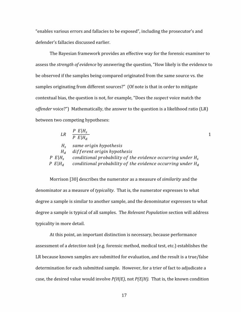
between two competing hypotheses:
𝐿𝐿𝐿𝐿 =𝑃𝑃(𝐸𝐸|𝐻𝐻𝑠𝑠)𝑃𝑃(𝐸𝐸|𝐻𝐻𝑑𝑑)
(1)
𝐻𝐻𝑠𝑠 = 𝑠𝑠𝑠𝑠𝑠𝑠𝑠𝑠 𝑜𝑜𝑜𝑜𝑜𝑜𝑜𝑜𝑜𝑜𝑜𝑜 ℎ𝑦𝑦𝑦𝑦𝑜𝑜𝑦𝑦ℎ𝑠𝑠𝑠𝑠𝑜𝑜𝑠𝑠𝐻𝐻𝑑𝑑 = 𝑑𝑑𝑜𝑜𝑑𝑑𝑑𝑑𝑠𝑠𝑜𝑜𝑠𝑠𝑜𝑜𝑦𝑦 𝑜𝑜𝑜𝑜𝑜𝑜𝑜𝑜𝑜𝑜𝑜𝑜 ℎ𝑦𝑦𝑦𝑦𝑜𝑜𝑦𝑦ℎ𝑠𝑠𝑠𝑠𝑜𝑜𝑠𝑠
𝑃𝑃(𝐸𝐸|𝐻𝐻𝑠𝑠) = 𝑐𝑐𝑜𝑜𝑜𝑜𝑑𝑑𝑜𝑜𝑦𝑦𝑜𝑜𝑜𝑜𝑜𝑜𝑠𝑠𝑐𝑐 𝑦𝑦𝑜𝑜𝑜𝑜𝑝𝑝𝑠𝑠𝑝𝑝𝑜𝑜𝑐𝑐𝑜𝑜𝑦𝑦𝑦𝑦 𝑜𝑜𝑑𝑑 𝑦𝑦ℎ𝑠𝑠 𝑠𝑠𝑒𝑒𝑜𝑜𝑑𝑑𝑠𝑠𝑜𝑜𝑐𝑐𝑠𝑠 𝑜𝑜𝑐𝑐𝑐𝑐𝑜𝑜𝑜𝑜𝑜𝑜𝑜𝑜𝑜𝑜𝑜𝑜 𝑜𝑜𝑜𝑜𝑑𝑑𝑠𝑠𝑜𝑜 𝐻𝐻𝑠𝑠𝑃𝑃(𝐸𝐸|𝐻𝐻𝑑𝑑) = 𝑐𝑐𝑜𝑜𝑜𝑜𝑑𝑑𝑜𝑜𝑦𝑦𝑜𝑜𝑜𝑜𝑜𝑜𝑠𝑠𝑐𝑐 𝑦𝑦𝑜𝑜𝑜𝑜𝑝𝑝𝑠𝑠𝑝𝑝𝑜𝑜𝑐𝑐𝑜𝑜𝑦𝑦𝑦𝑦 𝑜𝑜𝑑𝑑 𝑦𝑦ℎ𝑠𝑠 𝑠𝑠𝑒𝑒𝑜𝑜𝑑𝑑𝑠𝑠𝑜𝑜𝑐𝑐𝑠𝑠 𝑜𝑜𝑐𝑐𝑐𝑐𝑜𝑜𝑜𝑜𝑜𝑜𝑜𝑜𝑜𝑜𝑜𝑜 𝑜𝑜𝑜𝑜𝑑𝑑𝑠𝑠𝑜𝑜 𝐻𝐻𝑑𝑑
Morrison [30] describes the numerator as a measure of similarity and the
denominator as a measure of typicality. That is, the numerator expresses to what
degree a sample is similar to another sample, and the denominator expresses to what
degree a sample is typical of all samples. The Relevant Population section will address
typicality in more detail.
At this point, an important distinction is necessary, because performance
assessment of a detection task (e.g. forensic method, medical test, etc.) establishes the
LR because known samples are submitted for evaluation, and the result is a true/false
determination for each submitted sample. However, for a trier of fact to adjudicate a
case, the desired value would involve P(H|E), not P(E|H). That is, the known condition

18
is that the evidence has occurred and the desired output is the likelihood ratio of the
competing hypotheses. Confusing this inversion of probability is discussed in
Villejoubert [31], and is an underlying cause of the prosecutor’s fallacy.
Bayes’ Theorem delivers a solution to the inversion problem by providing a way
of converting results from the analysis results. Mathematically, the theorem is stated as
𝑃𝑃(𝐴𝐴|𝐵𝐵) =𝑃𝑃(𝐵𝐵|𝐴𝐴 ) × 𝑃𝑃(𝐴𝐴 )
𝑃𝑃(𝐵𝐵)(2)
Rewriting Equation (2) with notation from Equation (1) and substituting yields
Bayes’ Rule, the odds form of Bayes’ Theorem:
𝑃𝑃(𝐻𝐻𝑠𝑠|𝐸𝐸)𝑃𝑃(𝐻𝐻𝑑𝑑|𝐸𝐸) =
𝑃𝑃(𝐸𝐸|𝐻𝐻𝑠𝑠)𝑃𝑃(𝐸𝐸|𝐻𝐻𝑑𝑑) ×
𝑃𝑃(𝐻𝐻𝑠𝑠)𝑃𝑃(𝐻𝐻𝑑𝑑)
(3)
This form is particularly useful in presenting results of forensic analysis because
it isolates the contribution from the analysis in the overall adjudication of evidence.
The rightmost term is the prior odds, which represents the relative likelihood of Hs over
Hd before the evidence has been considered. The left side of the equation is the
posterior odds, which represents the relative likelihood after the evidence is considered.
Neither the prior or posterior odds are known by the forensic examiner, because they
aggregate the weight of other evidence in the case, and are not necessarily numeric
values (e.g. motive, eyewitness testimony, etc.). The left term on the right side of
Equation (3) is the likelihood ratio (sometimes referred to as the Bayes Factor, BF) from
Equation (1), and represents the strength of the given evidence. For example, if the LR
is computed as 10, then the trier of fact should be 10 times more likely to believe Hs
over Hd after considering the evidence than before considering the evidence.
19
Legal Foundations
Ultimately, the results of a forensic examination will be delivered to a decision
maker (e.g. to an attorney for a forensic case or to an investigator for an investigatory
case). At this point, the case essentially leaves the scientific realm and enters the legal
realm, with additional rules and conditions that apply. These rules are conceived with
the idea that only trustworthy evidence and testimony should be considered in an
adjudication. (In fact, Bronstein [21] dedicates an entire chapter to the best evidence
rule.) The Federal Rules of Evidence [32] codify the rules for United States federal
courts, and many states use these rules or similar rules for the state courts. The rules
are interpreted and applied as courts adjudicate cases, and the legal opinions expressed
in these cases become precedents that further prescribe how the legal system treats
forensic evidence and testimony.
Rules of Evidence
The Federal Rules of Evidence [32] is an extensive collection of rules for guiding
court procedures, and a few of the rules specifically relate to forensic evidence and
expert testimony. The following sections describe these rules with a brief commentary
as they relate to the scope of this document. The section, Federal Case Law, will address
how the adjudication process has clarified and extended these rules.

20
Rule 401 – Test for Relevant Evidence
Rule 401 – Test for Relevant Evidence Evidence is relevant if:
(a) it has any tendency to make a fact more or less probable than it would be without the evidence; and
(b) the fact is of consequence in determining the action.
While the technical results of a forensic examination may be relevant to a case,
the trier of fact may decide that the results are not relevant because, for example, they
are too technical for the judge or jury to understand. The testimony itself will not make
a fact more or less probable.
Rule 402 – General Admissibility of Relevant Evidence
Rule 402 – General Admissibility of Relevant Evidence Relevant evidence is admissible unless any of the following provides otherwise: • the United States Constitution; • a federal statute; • these rules; or • other rules prescribed by the Supreme Court. Irrelevant evidence is not admissible.
In conjunction with Rule 401, the results of a forensic examination would be
considered irrelevant if the evidence on which is based is declared to be inadmissible.
Rule 403 – Excluding Relevant Evidence
Rule 403 – Excluding Relevant Evidence for Prejudice, Confusion, Waste of Time, or Other Reasons The court may exclude relevant evidence if its probative value is substantially outweighed by a danger of one or more of the following: unfair prejudice, confusing the issues, misleading the jury, undue delay, wasting time, or needlessly presenting cumulative evidence.
If a forensic expert cannot express the results of an examination in an
understandable, unbiased, and efficient way, the testimony may be excluded.

21
Rule 702 – Testimony by Expert Witnesses
Rule 702 – Testimony by Expert Witnesses A witness who is qualified as an expert by knowledge, skill, experience, training, or education may testify in the form of an opinion or otherwise if:
(a) the expert’s scientific, technical, or other specialized knowledge will help the trier of fact to understand the evidence or to determine a fact in issue;
(b) the testimony is based on sufficient facts or data; (c) the testimony is the product of reliable principles and methods; and (d) the expert has reliably applied the principles and methods to the facts
of the case.
A forensic examiner must be considered an expert in the area of testimony, and
the principles involved in the testimony must be scientifically valid (e.g. researched by
the scientific method, peer reviewed by experts in the field, etc.). The expert must have
applied accepted methodologies during the examination process and reported the
results in a clear and unbiased manner. The primary goals of this rule is that expert
evidence must be relevant and reliable [33].
Rule 705 – Disclosing the Facts or Data Underlying an Expert’s Opinion
Rule 705 – Disclosing the Facts or Data Underlying an Expert’s Opinion Unless the court orders otherwise, an expert may state an opinion – and give the reasons for it – without first testifying to the underlying facts or data. But the expert may be required to disclose those facts or data on cross-examination.
The key point in this rule is that an expert is not required to present data to
support an expert opinion. However, the expert should be prepared to present such
information to avoid having that opinion invalidated or declared irrelevant. Having a
scientific basis for the testimony and following accepted practices provides the support
for withstanding a vigorous cross-examination.

22
Rule 901 – Authenticating or Identifying Evidence
Rule 901 – Authenticating or Identifying Evidence (a) IN GENERAL. To satisfy the requirement of authenticating or identifying
an item of evidence, the proponent must produce evidence sufficient to support a finding that the item is what the proponent claims it is.
(b) EXAMPLES. The following are examples only—not a complete list—of evidence that satisfies the requirement: … (3) Comparison by an Expert Witness or the Trier of Fact. A comparison with an authenticated specimen by an expert witness or the trier of fact. ... (5) Opinion About a Voice. An opinion identifying a person’s voice—whether heard firsthand or through mechanical or electronic transmission or recording—based on hearing the voice at any time under circumstances that connect it with the alleged speaker. … (9) Evidence About a Process or System. Evidence describing a process or system and showing that it produces an accurate result. …
A key point for Rule 901 is that an audio recording must be authenticated before
a forensic speaker comparison is relevant (which, as mentioned in the introduction, is
beyond the scope of this document). On the surface, example (5) would appear to give
explicit status to FSC, but in court cases [34], the example often is interpreted to imply
that human earwitness testimony is relevant (and admissible), therefore expert
testimony on FSC is not required. Example (9) may apply either to an FSC system being
used for analysis or to a system that is the actual evidence.
Federal Case Law
The following sections summarize the key points from a few of the significant
legal cases that have established requirements for the acceptance of forensic testimony.
The cases emphasize the rigorous scientific basis required for admissibility in court.

23
Frye v. United States
The Frye v. United States case [35] in 1923 established the principle of general
acceptance for forensic testimony. The ruling stated that the science and methods used
to form an expert opinion “must be sufficiently established to have gained general
acceptance in the particular field in which it belongs.” The Frye ruling became the
standard for expert testimony until Rule 702 effectively replaced it and changed the
focus to the reliability of the evidence. [36]
Daubert v. Merrell Dow Pharmaceuticals, Inc.
The Daubert case [37] established that Rule 702 superseded Frye, but also that it
was not sufficient. Expert testimony must be founded on “scientific knowledge” and
grounded in the methods and procedures of science (i.e. the scientific method). Thus,
the focus is on evidentiary reliability. The five principles given in the decision have
become known as the Daubert criteria [38]:
(1) whether the theories and techniques employed by the scientific expert have
been tested;
(2) whether they have been subjected to peer review and publication;
(3) whether the techniques employed by the expert have a known error rate;
(4) whether they are subject to standards governing their application; and
(5) whether the theories and techniques employed by the expert enjoy
widespread acceptance.
General Electric Co. v. Joiner
While Daubert ruled that the reliability of expert testimony should be based on
scientific principles and methodology, the GE v. Joiner case [39] extended this to say that

24
the conclusions reached must be based on the facts of the case to be relevant under
Rule 702. That is, an expert’s ipse dixit2 argument (i.e. “because I say so”) is not
sufficient. While the idea of a “conclusion” as described in this case is not equivalent to
the numerical result of an FSC algorithm, it does apply to the interpretation of the result
that is presented as an expert opinion. It also can apply to the expert’s interim
decisions during the analysis process, such as for the step of selecting a relevant
population, as detailed in the Analysis and Processing section of the framework.
United States v. McKeever
Rule 901 provides a general requirement for evidence to be authentic, and
specifically lists voice evidence as an example. The McKeever case [40] established a
foundation for this principle in its acceptance of a taped recording as being true and
accurate. While this case did not involve speaker recognition per se, it affects FSC in
that an examination may be deemed irrelevant if the audio evidence being analyzed is
not considered authentic.
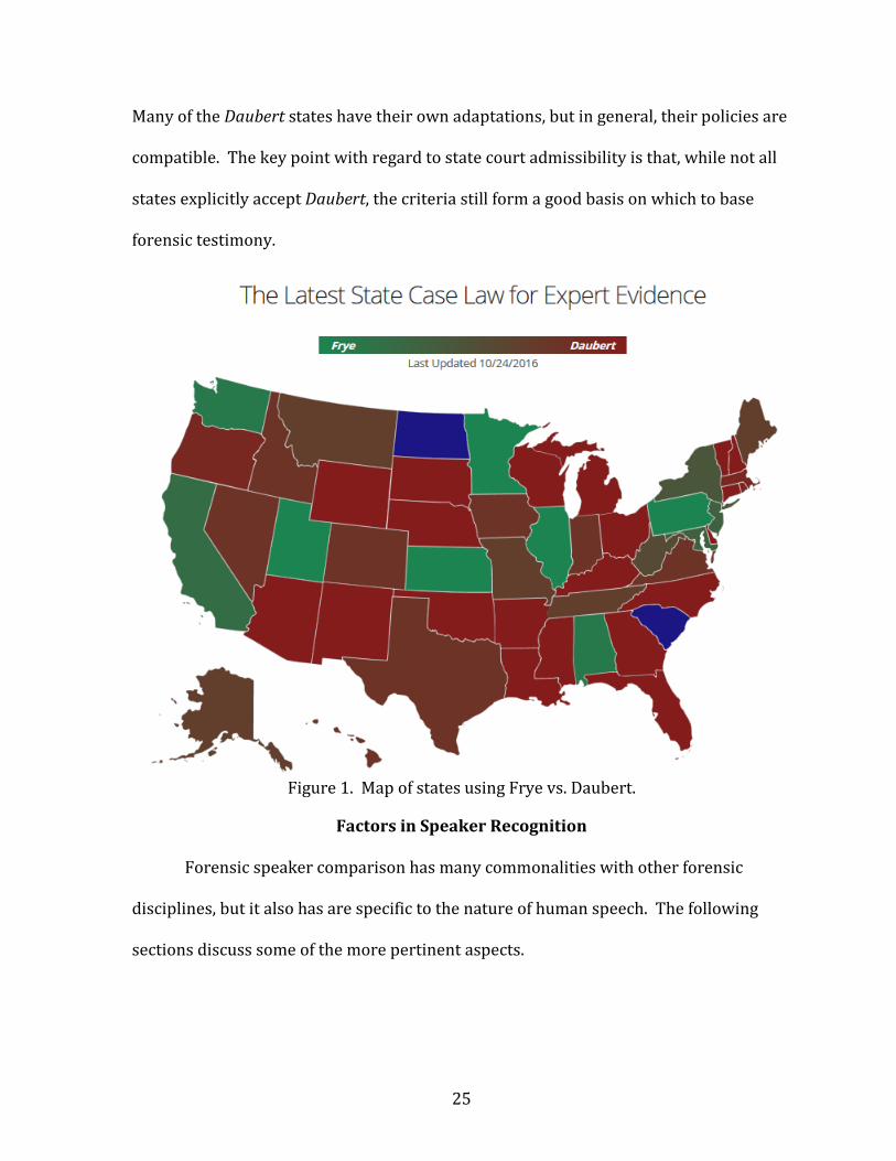
State Case Law
The standards for expert evidence vary between states, but all have legal
precedents directing its acceptance. Morgenstern [41] reports that as of 2016, 76% of
the states base their admissibility on Daubert, 16% use Frye, and the remaining 8% use
other guidance that, in most cases, can be considered to be essentially combination of
the two. The Jurilytics map [42] in Figure 1 shows the distinction not to be so clear.
2 Latin for “he himself said it”, referring to making an assertion without proof.
25
Many of the Daubert states have their own adaptations, but in general, their policies are
compatible. The key point with regard to state court admissibility is that, while not all
states explicitly accept Daubert, the criteria still form a good basis on which to base
forensic testimony.
Figure 1. Map of states using Frye vs. Daubert.
Factors in Speaker Recognition
Forensic speaker comparison has many commonalities with other forensic
disciplines, but it also has are specific to the nature of human speech. The following
sections discuss some of the more pertinent aspects.

26
The Nature of the Human Voice
For many forensic disciplines, the evidence primarily is dependent on the
physical traits of the actor from which the evidence originates (e.g. DNA, tire tracks,
etc.). A human voice sample, however, reflects not only the physical attributes of the
speaker, but also the behavior of the speaker and the conditions surrounding the
recording of the sample. During the analysis process when a questioned sample (Q) is
compared to a known sample (K), any mismatch conditions will complicate the
comparison. These differences can be intrinsic due to the words spoken, the state of the
speaker(s), etc., or extrinsic due to channel variations, differences in background or
recording conditions, etc. Table 2 illustrates the diversity of mismatch types with a
non-exhaustive list of conditions that can and often do cause mismatch between
samples. Intrinsic properties are those that derive from the behavior of the speaker
while the speech is created, while extrinsic properties are those that affect the speech
after it is produced.
Table 2. Potential Mismatch Conditions
Intrinsic Properties Extrinsic Properties Context Speaking
Style Vocal Effort
Physical State
Channel Background Recording Environment
Language Conversation Normal Excited Encoding Noise Small room Dialect Interview Shouting Angry Compression Environmental
Noise Reverberant
room Words spoken
Articulation rate
Whisper Physical activity
Sample Resolution
Overlapping speakers
Proximity to microphone
Time delay
Non-speech vocalization
Screaming Drug Effects
Sample Rate Non-speech events
Obscured speech
Culture Reading Preaching Stress Bandwidth Gender Preaching Fatigue Microphone
Disguise Illness Clipping Distortion

27
Modern algorithms have some degree of built-in compensation to adapt to these
mismatched conditions, but their performance in this regard is rather limited and is an
active area of research.
Speaker Recognition Systems
The following sections provide an overview of modern speaker recognition
systems. Most (if not all) modern automated speaker recognition systems are based on
supervised machine learning, which means that while algorithms in different systems
may be similar (or even identical), performance is heavily dependent on the data with
which the system is trained.
Under the Hood
Dete
ctio
nEn
rollm
ent
Feature Extraction
Model Library
Feature Extraction
Feature Extraction
Speaker Detection
Model Generation
Model Generation
Similarity Score
Known 1
Known 2
Questioned
Figure 2. Process flow for a typical speaker recognition system.
Figure 2 illustrates the general architecture of modern speaker recognition
system. In the enrollment phase, speech samples are submitted to the system, which

28
creates a model of the sample’s speech characteristics. Many systems make use of a
universal background model (UBM) that is trained on hundreds or thousands of hours
of speech recordings with the goal of generating a general model that captures the
common characteristics of a large population. For example, male and female voice
samples could be used separately to generate male-specific and female-specific UBMs.
Samples segregated by language could contribute to language-specific UBMs. Samples
from different microphone types or processed through different codecs could be used
to generate channel-specific UBMs. These specific UBMs, in theory, will give better
performance on those sample types for which they are tuned. For general use,
however, system designers often build a “kitchen sink” UBM from a balanced collection
of samples to give general all-around performance.
When individual speakers are enrolled into a system, algorithms model how the
given voice is different from the UBM. This normalization process furnishes a form of
mitigation for the base rate fallacy bias discussed in the Statistical Bias. Other forms of
normalization are implemented as well in an effort to adapt to non-speaker factors (e.g.
channel, language, gender, etc.).
In the scoring phase, a speech sample is compared against one or more speaker
models to measure its similarity. The comparison result can vary for different systems,
but typically is a likelihood ratio, log-likelihood ratio, or sometimes a raw score value
whose specific meaning is dependent on the algorithm that computed it. The likelihood
ratio framework is becoming the favored output, since it allows for a more direct
performance comparison between systems.
29
Evaluation of Speaker Recognition Systems
To address the data dependence for training automated speaker recognition
systems and to provide a standard baseline for researchers to test their ideas in a head-
to-head fashion, NIST periodically (approximately every two years) conducts a Speaker
Recognition Evaluation (SRE) [43] in which participating organizations may submit
results from their systems on a common set of test data. The tested systems primarily
are research-grade systems in order to test new ideas rather than turnkey systems
representing current product offerings. Conditions of the tests vary, but typically
include data sets with differing durations of speaker samples and mismatches in
channel conditions, language/dialect, etc. The protocols established by this competition
have become a common format for reporting system performance.
Evaluation of a system requires a data set that includes annotated (i.e. “truth
marked”) speech samples to identify the speaker from which the sample originated. A
portion of the data set is used during an enrollment phase to generate models for each
speaker in the data set. The remainder of the data set is then used during a scoring
phase in which the system computes a similarity score for each test sample against each
model. The scores for sample pairs that originate from the same speaker are known as
target scores, while the pairs from different speakers are non-target scores (or
sometimes, imposter scores). A high-performing system will produce high target scores
and low non-target scores, with statistically significant discrimination between the two
types. A perfect system would generate scores such that the minimum target score is
greater than the maximum non-target score. However, systems are hardly perfect,

30
because of inherent differences in the recognizability of different types of speakers.
Doddington [44] classifies these speakers as
• Sheep – the default speaker type that dominate the population. Systems
perform nominally well for them.
• Goats – speakers who are particularly difficult to recognize and account for a
disproportionate share of the missed detections.
• Lambs – speakers who are particularly easy to imitate and accounting for a
disproportionate share of the false alarms.
• Wolves –speakers who are particularly successful at imitating other speakers
and also account for a disproportionate share of the false alarms.
System with Good Discrimination
Figure 3 shows a plot of simulated score probability vs. score value for a system
with good discrimination of the data set being analyzed. The left histogram shows the
distribution of non-target scores, and the right shows target scores. The plotted curves
show the associated probability distributions of each score set modeled as Gaussian
(normal) distributions. At any point along the x-axis (i.e. the score from a comparison
of two samples), the ratio of the target probability to the non-target probability is the
likelihood ratio (LR) from Equation (1).

31
Figure 3. Simulated scores for a system with good discrimination.
Using a given score as a detection threshold, scores above that threshold would
be interpreted as detections, and scores below the threshold would be rejections. For
the non-target distribution, the scores below the threshold (the area under the curve to
the left of the threshold) are correct rejections, indicating that the two samples originate
from different speakers. The non-target scores above the threshold (the area to the
right of the threshold) are false alarms. For the target distribution, scores above the
threshold (the area to the right of the threshold) represent correct detections, or hits,
that the samples originate from the same speakers, while the scores below the
threshold are failed detections, or misses. The threshold value at which the false alarm
area equals the miss area is the equal error rate (EER) point, where the score is equally
likely to be a miss or a false alarm.
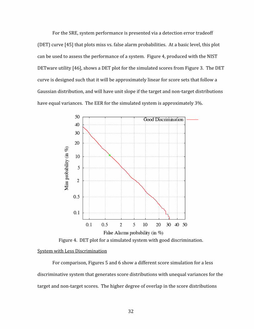
32
For the SRE, system performance is presented via a detection error tradeoff
(DET) curve [45] that plots miss vs. false alarm probabilities. At a basic level, this plot
can be used to assess the performance of a system. Figure 4, produced with the NIST
DETware utility [46], shows a DET plot for the simulated scores from Figure 3. The DET
curve is designed such that it will be approximately linear for score sets that follow a
Gaussian distribution, and will have unit slope if the target and non-target distributions
have equal variances. The EER for the simulated system is approximately 3%.
Figure 4. DET plot for a simulated system with good discrimination.
System with Less Discrimination
For comparison, Figures 5 and 6 show a different score simulation for a less
discriminative system that generates score distributions with unequal variances for the
target and non-target scores. The higher degree of overlap in the score distributions
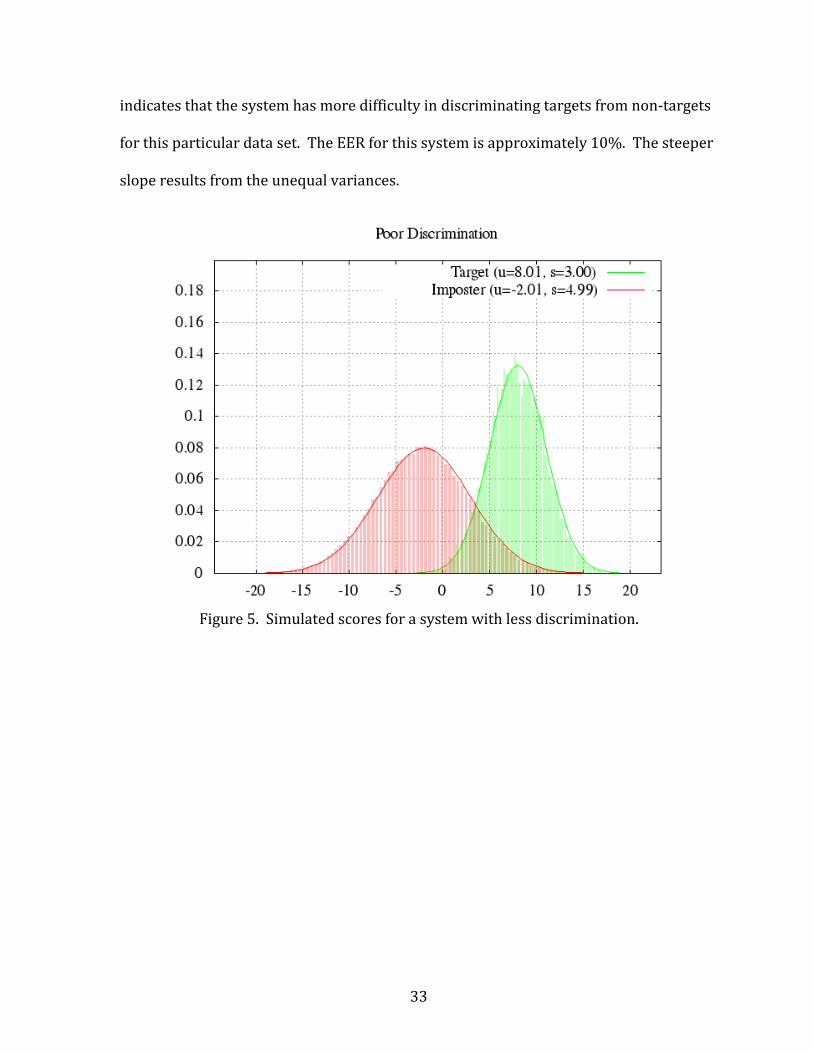
33
indicates that the system has more difficulty in discriminating targets from non-targets
for this particular data set. The EER for this system is approximately 10%. The steeper
slope results from the unequal variances.
Figure 5. Simulated scores for a system with less discrimination.

34
Figure 6. DET plot for a simulated system with less discrimination.
System with Minimal Data
Figures 7 and 8 show yet another score simulation to illustrate the impact of
data set size. The scores were generated using identical statistical parameters to the
first set, but the number of scores generated was much lower (10,000/100,000
target/non-target scores originally vs. 100/1000 for this set). Although the modeled
score distributions look similar to the previous plots, the jagged histograms reveal the
limited data behind the model, particularly at the sparse “tails” of the distribution. The
limited data set also results in a jagged DET plot. The EER should be approximately the
same for this data set as for the first data set, but the jagged plot does not clearly show
it.
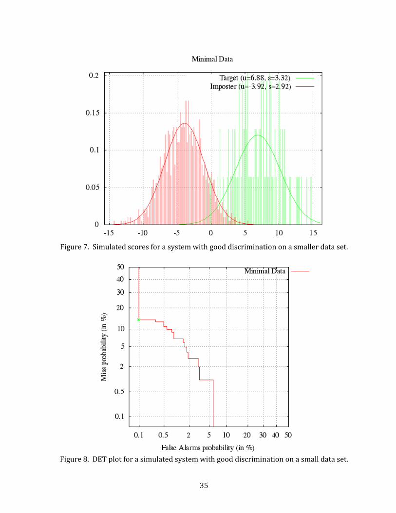
35
Figure 7. Simulated scores for a system with good discrimination on a smaller data set.
Figure 8. DET plot for a simulated system with good discrimination on a small data set.

36
System with Multimodal Distribution
Figures 9 and 10 show a multimodal simulation in which the non-target
distribution is a composite of scores generated from two different Gaussian
distributions. While this example is somewhat contrived, a similar condition could
occur if an examiner tried to compensate for a limited data set by augmenting it with
incompatible data. For example, adding cell phone data to landline data to avoid the
issue of minimal data in Figure 7 might result in such a multimodal score distribution
that no longer follows the Gaussian assumptions. The corresponding DET plot in Figure
10 is accordingly distorted so that it is no longer linear.
Figure 9. Simulated scores for a system with a multimodal non-target distribution.

37
Figure 10. DET plot for a simulated system with a multimodal non-target distribution.
System with Unrealistic Data
Finally, for purely illustrative purposes, Figures 11 and 12 show a simulation of
unrealistic scores. The non-target scores were generated using a triangular distribution
that, at first glance, resembles a Gaussian distribution. However, the triangular
distribution lacks the “tails” that result from unusually high or low outlying scores with
realistic data. The resulting nonlinearity of the DET plot reveals the atypical conditions.
While this example may seem a bit silly, similar conditions could conceivably occur if an
examiner, in an attempt to improve system performance, removed extreme score
values from the relevant population. Thus, the DET plot can be a valuable analysis tool,
not only to assess the accuracy of a system, but also to warn for the use of inappropriate
data or incorrect system operation.

38
Figure 11. Simulated scores for a system with triangular distributions.
Figure 12. DET plot for a simulated system with triangular score distributions.

39
Relevant Population
In the Mitigating Statistical Bias section, the likelihood ratio defined by Equation
(1) was given as measure of the strength of evidence for the results of a forensic
analysis. For FSC, the same origin hypothesis, Hs, becomes a same speaker hypothesis,
which should be a relatively straightforward definition. The different origin hypothesis,
Hd, similarly becomes a different speaker hypothesis, which is more problematic. FSC
systems actually assess similarities between samples, not differences, so how can a
system assess a different speaker hypothesis? The short answer is that it cannot.
However, it could, at least in theory, assess an any-other-speaker-in-the-world
hypothesis, Hworld. With these modifications, Equation (1) becomes
𝐿𝐿𝐿𝐿 =𝑃𝑃(𝐸𝐸|𝐻𝐻𝑠𝑠)
𝑃𝑃(𝐸𝐸|𝐻𝐻𝑤𝑤𝑤𝑤𝑤𝑤𝑤𝑤𝑑𝑑)(4)
𝐻𝐻𝑠𝑠 = 𝑠𝑠𝑠𝑠𝑠𝑠𝑠𝑠 𝑠𝑠𝑦𝑦𝑠𝑠𝑠𝑠𝑠𝑠𝑠𝑠𝑜𝑜 ℎ𝑦𝑦𝑦𝑦𝑜𝑜𝑦𝑦ℎ𝑠𝑠𝑠𝑠𝑜𝑜𝑠𝑠
𝐻𝐻𝑤𝑤𝑤𝑤𝑤𝑤𝑤𝑤𝑑𝑑 = 𝑠𝑠𝑜𝑜𝑦𝑦 𝑜𝑜𝑦𝑦ℎ𝑠𝑠𝑜𝑜 𝑠𝑠𝑦𝑦𝑠𝑠𝑠𝑠𝑠𝑠𝑠𝑠𝑜𝑜 𝑜𝑜𝑜𝑜 𝑦𝑦ℎ𝑠𝑠 𝑤𝑤𝑜𝑜𝑜𝑜𝑐𝑐𝑑𝑑 ℎ𝑦𝑦𝑦𝑦𝑜𝑜𝑦𝑦ℎ𝑠𝑠𝑠𝑠𝑜𝑜𝑠𝑠𝑃𝑃(𝐸𝐸|𝐻𝐻𝑠𝑠) = 𝑐𝑐𝑜𝑜𝑜𝑜𝑑𝑑𝑜𝑜𝑦𝑦𝑜𝑜𝑜𝑜𝑜𝑜𝑠𝑠𝑐𝑐 𝑦𝑦𝑜𝑜𝑜𝑜𝑝𝑝𝑠𝑠𝑝𝑝𝑜𝑜𝑐𝑐𝑜𝑜𝑦𝑦𝑦𝑦 𝑜𝑜𝑑𝑑 𝑦𝑦ℎ𝑠𝑠 𝑠𝑠𝑒𝑒𝑜𝑜𝑑𝑑𝑠𝑠𝑜𝑜𝑐𝑐𝑠𝑠 𝑜𝑜𝑐𝑐𝑐𝑐𝑜𝑜𝑜𝑜𝑜𝑜𝑜𝑜𝑜𝑜𝑜𝑜 𝑜𝑜𝑜𝑜𝑑𝑑𝑠𝑠𝑜𝑜 𝐻𝐻𝑠𝑠
𝑃𝑃(𝐸𝐸|𝐻𝐻𝑤𝑤𝑤𝑤𝑤𝑤𝑤𝑤𝑑𝑑) = 𝑐𝑐𝑜𝑜𝑜𝑜𝑑𝑑𝑜𝑜𝑦𝑦𝑜𝑜𝑜𝑜𝑜𝑜𝑠𝑠𝑐𝑐 𝑦𝑦𝑜𝑜𝑜𝑜𝑝𝑝𝑠𝑠𝑝𝑝𝑜𝑜𝑐𝑐𝑜𝑜𝑦𝑦𝑦𝑦 𝑜𝑜𝑑𝑑 𝑦𝑦ℎ𝑠𝑠 𝑠𝑠𝑒𝑒𝑜𝑜𝑑𝑑𝑠𝑠𝑜𝑜𝑐𝑐𝑠𝑠 𝑜𝑜𝑐𝑐𝑐𝑐𝑜𝑜𝑜𝑜𝑜𝑜𝑜𝑜𝑜𝑜𝑜𝑜 𝑜𝑜𝑜𝑜𝑑𝑑𝑠𝑠𝑜𝑜 𝐻𝐻𝑤𝑤𝑤𝑤𝑤𝑤𝑤𝑤𝑑𝑑
This equation is not particularly useful in its current form, because with
approximately six billion humans on the planet, the feasibility of calculating P(E|Hworld)
is essentially zero. However, the Law of Total Probability given in Equation (5) can
address the issue by partitioning P(E|Hworld) into smaller segments.
𝑃𝑃(𝐴𝐴) = �𝑃𝑃(𝐴𝐴|𝐵𝐵𝑖𝑖)𝑃𝑃(𝐵𝐵𝑖𝑖 )𝑖𝑖
(5)
For example, P(E|Hworld) could be partitioned by countries, yielding
𝑃𝑃(𝐸𝐸|𝐻𝐻𝑤𝑤𝑤𝑤𝑤𝑤𝑤𝑤𝑑𝑑) = 𝑃𝑃�𝐸𝐸�𝐻𝐻𝐴𝐴𝐴𝐴𝐴𝐴ℎ𝑎𝑎𝑎𝑎𝑖𝑖𝑠𝑠𝑎𝑎𝑎𝑎𝑎𝑎�𝑃𝑃�𝐻𝐻𝐴𝐴𝐴𝐴𝐴𝐴ℎ𝑎𝑎𝑎𝑎𝑖𝑖𝑠𝑠𝑎𝑎𝑎𝑎𝑎𝑎 � (6)+ 𝑃𝑃(𝐸𝐸|𝐻𝐻𝐴𝐴𝑤𝑤𝐴𝐴𝑎𝑎𝑎𝑎𝑖𝑖𝑎𝑎)𝑃𝑃(𝐻𝐻𝐴𝐴𝑤𝑤𝐴𝐴𝑎𝑎𝑎𝑎𝑖𝑖𝑎𝑎 )+⋯ + 𝑃𝑃(𝐸𝐸|𝐻𝐻𝑍𝑍𝑖𝑖𝑍𝑍𝐴𝐴𝑎𝑎𝐴𝐴𝑤𝑤𝑍𝑍)𝑃𝑃(𝐻𝐻𝑍𝑍𝑖𝑖𝑍𝑍𝐴𝐴𝑎𝑎𝐴𝐴𝑤𝑤𝑍𝑍 )

40
Assuming that the probability of the speaker being from any other country than,
e.g., the United States, is zero, Equation (6) simplifies to
𝑃𝑃(𝐸𝐸|𝐻𝐻𝑤𝑤𝑤𝑤𝑤𝑤𝑤𝑤𝑑𝑑) = 𝑃𝑃(𝐸𝐸|𝐻𝐻𝑈𝑈𝑎𝑎𝑖𝑖𝑎𝑎𝑍𝑍𝑑𝑑𝑈𝑈𝑎𝑎𝑎𝑎𝑎𝑎𝑍𝑍𝑠𝑠)𝑃𝑃(𝐻𝐻𝑈𝑈𝑎𝑎𝑖𝑖𝑎𝑎𝑍𝑍𝑑𝑑𝑈𝑈𝑎𝑎𝑎𝑎𝑎𝑎𝑍𝑍𝑠𝑠 ) (7)
Further partitioning is possible by eliminating more groups for which the
evidence would be have zero probability of occurring, with an ultimate result of
something like
𝑃𝑃(𝐸𝐸|𝐻𝐻𝑤𝑤𝑤𝑤𝑤𝑤𝑤𝑤𝑑𝑑) = 𝑃𝑃�𝐸𝐸�𝐻𝐻𝑈𝑈𝑆𝑆𝑎𝑎𝑎𝑎𝑖𝑖𝑠𝑠ℎ𝑈𝑈𝑆𝑆𝑍𝑍𝑎𝑎𝑆𝑆𝑍𝑍𝑤𝑤𝑆𝑆𝑎𝑎𝑆𝑆ℎ𝑍𝑍𝑒𝑒𝑤𝑤𝑤𝑤𝑍𝑍�𝑃𝑃�𝐻𝐻𝑈𝑈𝑆𝑆𝑎𝑎𝑎𝑎𝑖𝑖𝑠𝑠ℎ𝑈𝑈𝑆𝑆𝑍𝑍𝑎𝑎𝑆𝑆𝑍𝑍𝑤𝑤𝑠𝑠𝑆𝑆𝑎𝑎𝑆𝑆ℎ𝑍𝑍𝑒𝑒𝑤𝑤𝑤𝑤𝑍𝑍 � (8)
This partitioning is the general idea behind the relevant population, and
comparing a voice sample to a set of samples similar to the sample in question
addresses the typicality mentioned in Mitigating Statistical Bias. In addition to the idea
of language similarity in the previous example, this concept also extends to include
mismatch conditions from Table 2. For example, if a sample in evidence contains
unstressed conversational Arabic speech with an Egyptian accent, the relevant
population should include samples with those characteristics (or at least as many as
possible). Ultimately, selection of a relevant population is dependent on the judgement
of an examiner, which highlights the importance of examiner training, accepted
procedures, and ethical standards.
Bias Effects
For many forensic disciplines, examination of the evidence is not, by itself, likely
to bias an examiner. For example, a DNA or fingerprint analysis is unlikely to cause an
examiner to prejudge the originator of the evidence as “guilty” based solely on carrying
out the analysis process. However, the act of listening to the audio recording of a crime
as part of the analysis can affect an examiner’s conclusions due to cognitive bias.

41
Standards
While some individual forensic laboratories have procedures for performing
forensic speaker comparisons, no widely accepted standards exist. The OSAC-SR
subcommittee is actively developing best practices and guidelines, but the current
schedule currently envisions a mid-2018 publication.
Historical Baggage
Modern speaker recognition technology has grappled with the consequences of
public misconceptions stemming from earlier technology whose capability was over-
promoted. In 1962, Kerst [47] proclaimed:
Previously reported work demonstrated that a high degree of speaker identification accuracy could be achieved by visually matching the Voiceprint (spectrogram) of an unknown speaker's utterance with a similar Voiceprint in a group of reference prints.
Just five years later in 1967, Vanderslice and Ladefoged [48] countered with:
Proponents of the use of so-called "voiceprints" for identifying criminals have succeeded in hoodwinking the press, the public, and the law with claims of infallibility that have never been supported by valid scientific tests. The reported experiments comprised matching from sample – subjects compared test "voiceprints" (segments from wideband spectrograms) with examples known to include the same speaker – whereas law enforcement cases entail absolute judgment of whether a known and unknown voice are the same or different. There is no evidence that anyone can do this.
Subsequent legal proceedings have concurred with both sides of the discussion,
but the prevailing trend is that “voiceprints” in the form of spectrograms have fallen
into disfavor in recent years. In US v. Bahena [49], the particular voice spectrographic
testimony used was deemed unreliable, and the decision in US v. Angleton [50] ruled
similarly:
42
The government contends that the aural spectrographic method for voice identification in general, and Cain's application of that method in particular, do not meet the Rule 702 and Daubert standards of admissibility.
Despite some continued use of voiceprints by smaller labs (who no doubt have a
vested interest in continuing the practice as part of their business models), larger
accredited labs are moving toward human-supervised automated methods. Perhaps
most significant is that in the past few years, the FBI has stopped using voiceprints as a
standard practice [51].
Another method of speaker recognition, aural-perceptual (sometimes called,
“critical listening” ) has been employed by experts who claim to be proficient, but often
have not offered results of validation testing to prove their claims. In the Zimmerman
case [51], Dr. Nakasone testified that the practice is used at the FBI laboratory, but only
in conjunction with automated probabilistic methods. Rule 901 notwithstanding, it is a
very subjective method, and as such, can be highly susceptible to cognitive bias and
error.
43
CHAPTER III
COMPARISON FRAMEWORK
The position of this paper is that to the extent possible, an examination should
be conducted with all due rigor as if it will be challenged in court, even in an
investigatory setting in which that ultimate result is not likely. The proposed
framework depicted in Figure 13 consists of three phases that encompass several steps.
To focus on the comparison methodology, certain aspects of the process common to
most forensic disciplines are expected. For example, assumptions include:
• Relevant standard operation procedures (either community-wide or lab-
specific) will be followed.
• All examiners will be properly trained for the tasks being performed.
• Lab personnel that handle the evidence will follow established chain of
evidence and preservation practices.
• Analysis steps with accompanying reasons will be documented during the
examination. (This is particularly important with challenging cases to be
able to defend against allegations of tailoring the examination to obtain a
desired result.)
• Methods and/or tools used during the examination will have been properly
vetted through accepted validation and verification (V&V) procedures and
can provide known error rates. (See Daubert criteria in the Federal Case Law
section)

44
Case Assessment
Analysis and Processing
Case Conclusions
Administrative Assessment
Technical Assessment
Data Enhancement
Relevant Population
System Performance
HandlingResults
Interpreting Results
Communicating Results
Figure 13. Framework flowchart for forensic speaker comparison.
Case Assessment
The Case Assessment phase begins when a forensic request is received and
concludes when laboratory personnel determine that
• the evidence provided is sufficient in terms of quality, quantity, and format to
justify an examination
• the laboratory has the resources (i.e. availability of qualified examiners,
appropriate tools, and suitable reference data) for the analysis requested
• a proper forensic question (or questions) can be formulated to satisfy the
needs of the requestor.

45
Forensic Request
Each laboratory should establish a formal process through which personnel
interact with the requestor. Ideally, a forensic request arriving at a laboratory should
be handled by a case manager who is responsible for capturing information regarding
the case and interacting with the requestor, but will shield the assigned examiner from
potentially biasing information. Even simple information about the requestor could
influence the examiner. For example, knowing the request is from a law enforcement
agency might lead the examiner to consider the sample of interest to be from a
“suspect”, or examiners may interpret evidence differently based on their preference
for one client over another. On the other hand, maintaining an objective process may
enhance an attorney’s strategy for a case by proving the impartiality of the analysis.
For labs where having a case manager is not practical, access to information
provided by the requestor should be limited, for example, by placing different
categories of information on different pages of a case request form, and by providing
instructions for the form should that explain how to populate the form without biasing
the analysis. General information should include administrative fields such as:
• Case reference number
• Date/time of request
• Date/time that the evidence should be returned
Technical information that could aid (but not bias) the examiner in performing
the analysis might include fields such as:
• Evidence reference information and file names (for digital formats). Samples
for analysis should be listed as questioned (Q1, Q2, …) or known (K1, K2, …).

46
If known, the identity should be included with actual names masked, as the
case requires. Any aliases used should be benign terms, not pejorative ones
(e.g. “narrator”, “interviewer”, etc. rather than “suspect”, “victim”, or “perp”).
• Media information, such as the source device, if known, of the samples. For
example, knowing that a sample originated from a particular brand of
audio/video surveillance equipment, a telephone wiretap, or a desktop
microphone in a reverberant interview room might prove useful during the
analysis. The information provided should be considered carefully, as some
information (such as the body microphone case mentioned in the Mitigating
Cognitive Bias section) might be a source of bias.
Other potentially biasing information should only be available to a case manager
and revealed to an examiner as needed (i.e. sequential unmasking as per Inman [26]):
• Requestor of case and contact information. Knowing whether the request
originates from law enforcement or from the prosecution/defense attorney
may bias the examination.
• Chain of custody records – delivered by, date/time, etc. Knowing this
information could reveal the requestor.
• Purpose of examination – criminal/civil case, corporate investigation, etc.
Included in this category is information regarding legal theories or
Administrative Assessment
The administrative assessment is a straightforward process that makes an initial
determination as to whether the laboratory is capable of performing the requested
analysis.

47
Evidence Handling
Acceptance of evidence for analysis must follow best evidence principles. For
example, if the audio quality of a received speech sample is inferior to an original
version, then the original should be procured for analysis if possible. As another
example, edited versions of a digital audio sample should not be accepted for
processing without full disclosure as to the nature of the sample. All evidence handling
throughout the examination must be conducted in accordance with relevant laboratory
standards, and should adhere to the Fundamental Principle [52] of digital and
multimedia forensics, which is to “maintain the integrity and provenance of media upon
seizure and throughout processing.”
Analysis Capability
Case evidence must be assessed with respect to the capabilities of the
laboratory. General qualifications for a forensic laboratory may be addressed by the
following example questions:
• Does the case involve any conflict of interest or other ethical issues that
preclude involvement of the laboratory or its personnel in the requested
analysis?
• Are laboratory personnel properly trained for the required operations?
• Are the laboratory personnel competent to perform the requested analysis?
Beyond any specific training requirements, are special certifications or
accreditations required?
• Does the case or its evidence impose special security constraints or require
specialized evidence handling beyond the normal procedures?
48
Additional specific laboratory qualifications for performing forensic speaker
comparisons should be addressed as well:
• Is the evidence in a format that is supported by laboratory equipment? For
example, analog audio evidence will require optimized playback and digital
capture. For FSC, video formats will require extraction of the audio signal for
analysis.
• Is language consultation available if the need arises during analysis?
• Does the laboratory have appropriate data that may serve as a relevant
population for the evidence provided? (This check is only a preliminary
assessment regarding the data inventory for the laboratory. Actual selection
of data for the relevant population will be covered in Analysis and Processing,
below.)
Forensic Question
The forensic question must be crafted in a form that the analysis process can
answer. It cannot, for example, ask whether a suspect is guilty, or whether a questioned
sample “matches” a known sample with one hundred percent accuracy. Since the FSC
process compares questioned samples against known samples, a proper forensic
question, therefore, must address the similarities and differences revealed during the
analysis process and evaluate the weight of the evidence as measured by those
similarities and differences. A proper question, then, might be:
How likely are the observed measurements between the questioned and known samples if the samples originated from the same source vs. the samples originating from different sources?
49
The output of automated systems is typically an uncalibrated score or a
calibrated likelihood (or log-likelihood) ratio. Traditionally, the value is higher for
same-origin samples and lower for different-origin samples, so it provides a measure of
similarity between the samples.
For simplicity, the comparison task in this paper will be framed as a one-to-one
comparison of two samples, typically labeled as questioned (Q) and known (K). (Even if
the origin of neither is known, they may be treated in this manner for analysis
purposes.) One-to-many or many-to-many cases are an extension of the one-to-one
case. A proper forensic request for the one-to-one case should be framed so that the
strength of evidence, as discussed in the section Mitigating Statistical Bias can be
answered by the likelihood ratio (LR) from Equation (1). The evidence, E, essentially is
the measured similarity calculated by the speaker recognition algorithm. The
numerator and denominator become, respectively,
• the probability of obtaining the observed similarities in Q and K if the
samples originated from the same source
• the probability of obtaining the observed similarities in Q and K if the source
of Q was some other randomly selected sample in the relevant population.
The actual numerator and denominator are not typically witnessed outside the
tool, as the actual ratio is reported.
Technical Assessment
The technical assessment begins the analysis process on the actual content of the
evidence. Once the samples arrive into the laboratory environment, the examiner
50
conducts and documents a series of qualitative and quantitative measurements
arranged into three phases:
• subjective analysis (i.e. listening tests) by the examiner
• objective analysis by automated tools
• comparison of the subjective and objective results by the examiner
The order of operations is critical to minimize bias influences. The examiner
should not know the results from the automated tools before performing the subjective
analysis. In addition, questioned samples (Q) should be evaluated before known
samples (K) so that contextual bias does not influence the detection of K sample
characteristics in the Q sample. Finally, an aggregation of the individual analysis results
contributes to the ultimate decision to proceed with a full analysis
Data Ingest
FSC algorithms typically accept digital, uncompressed recordings as input, but
the Q and K samples for the case often arrive in an incompatible format. Analog
recordings, for example, must be digitized into a format compatible with the tools to be
used. To obtain the highest quality results (i.e. the best evidence), the playback
equipment must be configured for optimum fidelity. This operation is outside the scope
of this document, but the SWGDE guidelines [5] provide a good reference.
Digital samples arriving as ordinary audio files (e.g. .wav, .mp3, etc.) often can be
analyzed directly, but must first undergo screening per laboratory policies to scan for
computer viruses, compute message digest values for documenting the evidence, etc.
Digital audio may also arrive as a component of a multimedia recording. For example, a
speaker sample may require the extraction of an audio track from a video file. Digital

51
audio samples in a media format (e.g. digital audio tape, compact disc, etc.) must
undergo an acquisition step to convert the samples into computer files. For example,
the audio tracks from compact discs must be “ripped” from the CD into files.
All software tools, equipment, and processes used for ingest must, of course, be
validated for the operations being performed.
Subjective Analysis
The subjective analysis requires the examiner to listen to the audio samples (Q
before K) to document noteworthy characteristics. The intrinsic and extrinsic mismatch
conditions from Table 2 provide a diverse starting set. Because this phase is dependent
on examiner knowledge and experience, it may necessitate consultation with other
examiners to yield comprehensive results across all conditions. Results typically are
more qualitative than quantitative in nature, but still are useful in evaluating mismatch
conditions.
Examiners should take particular note of characteristics for which automated
tools are available to analyze. Having both types of analysis for a given characteristic
allows for later comparison and cross-checking after all analyses are complete. For
example, Ramirez [53] reports on small effects from clipping distortion that can have a
significant impact on the performance of speaker recognition algorithms due to the
spectral distortion created. Clipping can be relatively easy to detect simply by listening
to a recording, and some audio editors have analysis capabilities to detect clipping. As
another example, background events such as bird calls should be detected for later
removal. An examiner may detect such events by listening, and the results of
automated algorithms [54] [55] can be used for comparison.

52
Objective Analysis
Generally speaking, tools that can evaluate extrinsic conditions are more
common than tools for intrinsic conditions because more data is available with which to
conduct experiments and develop the tools. Researchers can easily collect voice
samples by, say, setting up multiple microphones and encoding the data with different
codecs to create data under varied extrinsic conditions. However, creating an
equivalent data set with intrinsic variation requires multilingual speakers, speakers in
varying emotional or physical states, speakers under different external influences, etc.
Additionally, annotating such a data set is problematic because it requires manual entry
of the annotations. The development of automated metrics for identifying the different
conditions would greatly facilitate the development of such data sets.
Tools such as the MediaInfo [56] utility can be useful for extracting and reporting
sample metadata such as duration, bit depth, sample rate, encoding format, etc.
Analytical tools such as the Speech Quality Assurance (SPQA) package from the NIST
Tools web site [57] can be used to detect clipping distortion and to evaluate the signal-
to-noise ratio (SNR ) in speech samples. While the actual calculation method of SNR is a
subject of debate, generating the value in a consistent way is useful as a metric for
comparison of sample mismatch.
Tools that evaluate intrinsic conditions are beginning to emerge as researchers
leverage machine learning algorithms trained on data sets organized by various
conditions. For example, the case studies in the paper will use a system that uses
training data organized by gender and language to evaluate samples. The system also
uses data organized by microphone, codec, and general perceived degradation levels to
53
evaluate extrinsic characteristics. Of note is that, for example, the codec evaluation is
not based on metadata stored in the sample file; it is based on audio characteristics that
are similar to the training data encoded with different codecs. Even if the sample is
converted to a different format, the audio characteristic remain and can be detected.
Evaluation of audio evidence according to these categories, then, can assist in
determining mismatch conditions in an objective way. Additionally, the language
detection feature can be useful to alert an examiner to a potential need for language
resources.
Comparison of Analysis Results
The comparison of the subjective and objective results provides a “sanity check”,
of sorts, on both the examiner judgements and the proper operation of the tools used.
Any results that differ for common characteristics should be investigated thoroughly.
For example, if an examiner assesses the Q and K languages to be Arabic/Arabic
(without necessarily being qualified as an Arabic linguist) and a language recognition
tool assesses the languages as Arabic/Urdu, language consultation may be required. A
finding that the tool is incorrect may give insight into other potential mismatch
conditions (e.g. the tool may, for example, be confusing codec or distortion effects with
language differences). These differences are relevant for the selection of a relevant
population later.
Decision to Proceed with Analysis
After the administrative and technical assessments have concluded that the
evidence can be processed, the examiner must decide whether it should be processed.
54
In addition to assessing the evidence mismatch conditions from Table 2, the examiner
must assess potential mismatches between the evidence and the requirements for any
system(s) being used to perform the FSC. Such mismatches may dictate that the case be
rejected (i.e. punted [58]), and may include, but are not limited to, the following
conditions:
• Duration – Does the FSC system require a minimum duration to meet
performance levels for which it was validated? (As a side note, this
requirement is not satisfied by repeating a shorter recording to extend its
duration.)
• Training data mismatch – Are the attributes of the underlying data with
which the FSC system was trained known to the examiner? For example, did
the system come from the vendor trained with English, landline audio
samples? Broadcast quality audio? An understanding of the tool, its
limitations, and the conditions for which it is validated is vital.
• Evidence quality – Are the evidence recordings of sufficient quality for the
system to analyze properly? For example, will a noisy signal cause errors in
the voice activity detection of the system? If the system cannot detect the
voice segments accurately, it cannot possible provide reliable results.
At the current level of technology, assessment of these conditions is a subjective
decision on the part of the examiner and requires thorough documentation of the
decisions made. For investigatory cases, the bar may be set a bit lower with the
understanding that the results should be evaluated with an appropriate level of
skepticism and cross-validated where possible.
55
As a final check, an examiner should revisit the relevant population issue
discussed earlier in the Administrative Assessment section. The actual selection will
occur in the Analysis and Processing section, below, but the availability of suitable data
contributes to the decision to continue the analysis.
After the technical assessment, more details are known about the evidence and a
better decision can be made with respect to the data available. For example, the
relevant population often is selected intuitively with the assumption that the language
and/or dialect of the evidence are key attributes to match. However, little scientific
research supports this decision for data in other than laboratory research conditions.
Other attributes (e.g. the conditions in Table 2) may be important for the selection of
the relevant population, but more research is necessary to better understand this
process. In any case, the system should be validated for performance with the selected
relevant population. From the guidelines published by the European Network of
Forensic Science Institutes (ENFSI) [59]:
If system requirements for a given FASR or FSASR method are not met, it can be considered whether a new database can be compiled or whether an existing database can be adapted and evaluated in a way that the quality and quantity profile of the case is met. In that case it is important that a test is performed on this new or modified test set and that performance characteristics and metrics are derived that are analogous to a full method validation (chapter 4). The only difference from a full method validation would be that such a more case-specific testing and evaluation does not contain a validation criterion.
Analysis and Processing
The Analysis and Processing phase is consists of readying voice samples for
analysis, submitting them to an FSC system for analysis, and managing the results.
While this document focuses on automated methods, the framework itself is agnostic to

56
the specific choice of method, as long as the result is a numerical value that provides a
similarity measure for the compared samples.
Data Preparation
The Data Preparation step of a voice sample for analysis is a selection process
that extracts audio segments for submission to an FSC system. The process is also
called purification, because the goal is to remove audio that is not characteristic of the
speaker of interest. For example, vocalizations such as coughs, sneezes, throat clearing,
etc. should be edited out. Background sounds such as bird calls, dog barks, slamming
doors, etc. similarly should be removed. The resulting audio from the edits must be of
sufficient duration to meet the minimum duration requirements for the analysis tools.
Under no circumstances should audio be repeated (i.e. “looped”) to satisfy the duration
requirement. All edits and the reasons for them should be documented thoroughly,
particularly if the segments removed involve idiosyncratic vocalizations that would, as
a subjective observation, contribute to the overall voice comparison.
Recordings that contain multiple modes of speech (e.g. language “code
switching”, speaking style variations, environment changes, microphone proximity
differences, etc.) should be segmented into separate samples for each mode and
submitted separately for analysis. (That is, sample Q1 becomes Q1a, Q1b, Q1c, etc.)
Each sample must individually satisfy the minimum duration requirements for analysis.
For example, a recording in which a speaker is speaking English indoors, becomes
angry, walks outside, and switches to Spanish should be split into four segments:
“English-indoor-calm”, “English-indoor-angry”, “English-outdoor-angry”, and “Spanish-
outdoor-angry”.
57
Finally, longer duration samples may be split into multiple segments to verify
reasonable behavior of the analysis system. Sample segments that otherwise seem to
have equivalent conditions should score similarly; if not, the examiner must investigate
and resolve the discrepancy before issuing a report.
Data Enhancement
While the Data Preparation step selects audio content for analysis, the Data
Enhancement step actually modifies the audio content. Such modifications should
follow accepted forensic audio practices and standards. For FSC in particular, any
enhancement must be made with extreme care and with proper validation testing to
assess the impact of the modifications on the FSC systems. For example, filtering
operations to remove tones or hum, or simply to make an audio recording easier for a
human to listen to could very well remove critical audio characteristic on which an FSC
system depends for proper operation. For any uncertainty as to the effect of a
particular enhancement, both the original sample and the enhanced sample should be
submitted to the FSC system to compare the results.
Modifications in the opposite direction to add noise, in general, are discouraged.
For example, linearly adding noise to a clean audio recording of a speaker to simulate a
noisy recording will give different results from recording speech in a noisy environment
due to nonlinear interactions between the voice and the environment.
The application of any enhancement operations should be guided by the
following principles:
• All operations, algorithm settings, etc. must be thoroughly documented.
• The limitations of tools used must be fully understood.
58
• Any enhancements must be validated as to their effect on the performance of
FSC algorithms.
Selection of the Relevant Population
The selection of a relevant population (or more precisely, the sampling of the
relevant population) is perhaps the most important step in the analysis process, and a
highly subjective one at the current state of technology. The selection is analogous to a
traditional “line-up” in which a witness is asked to view a set of potential suspects that
match the description given by the witness. If the witness has stated that the suspect
was six feet tall, had brown hair, and was wearing blue jeans and a T-shirt, then the
line-up would consist of suspects matching that description. Selection of a “voice line-
up” is similar in that voice samples from a database are selected that have similar
characteristics (e.g. the mismatch conditions from Table 2) to the questioned and/or
known voices. The results from the subjective and objective analyses from the
Technical Assessment section are used to select the population.
This step can critical to a successful examination. If no sufficiently similar voice
samples are available, the analysis cannot be completed. Matching all the data
conditions often is only possible for straightforward circumstances such as same-
language telephone recordings over the same or similar channels, recordings in a quiet,
non-reverberant room, etc. The paradox in the selection process is that limiting the
selection by matching as many conditions as possible reduces the statistical content of
the population. Allowing a broader selection to improve the statistics risks
incorporating more mismatched data in the population and, therefore, making it less
relevant.

59
Although tools are beginning to emerge (as discussed in the Objective Analysis
section) to objectively assess sample characteristics and thus aid in the selection
process, the current practice often is a subjective process and focuses on mismatch
conditions for which data is available. For example, a relevant population might be
selected to match the language or channel conditions of the evidence sample simply
because multilingual and multichannel corpora are available. Mismatch conditions such
as reading/preaching, angry/calm, or old/young [60] are more of a challenge due to the
lack of data supporting those conditions.
The selection of a relevant population is the partitioning process discussed in the
Relevant Population section that reduces P(E|Hworld) to a manageable entity. Ultimately,
the selected population must be accepted by the trier of fact (or decision maker), who
must be satisfied that sufficiently represents the typicality of the evidence samples.
System Performance and Calibration
Calibration of systems for FSC is a statistical process that requires a relatively
large data set of annotated voice samples for which speaker identities are known.
Additionally, the i-Vector and PLDA algorithms used in recent systems assume a
homogeneous distribution of training, so the data set should not be extended by, for
example, combining samples from multiple collections. (Such a combination potentially
could result in a multimodal distribution as discussed earlier.) Turnkey systems may
incorporate standard calibration settings for common conditions, but the examiner
should be familiar with these settings and the conditions for use. This knowledge
directly contributes to the decision at the end of the case assessment phase to continue
with an analysis.

60
For conditions not explicitly supported by a prebuilt system configuration, an
examiner must assess whether the mismatched conditions are similar enough to
warrant use of a prebuild configuration. Unfortunately, the quantification of the
mismatch is an unsolved problem in the research, and the mismatch assessment is a
subjective judgement. The decision is highly dependent on the system and the case
evidence and must, of course, be documented in the analysis. The decision to continue
analysis must include a validation for the case conditions. For example, a system
trained on English landline telephone recordings might be used to analyze Spanish
landline telephone recordings if a sufficient quantity of similar annotated Spanish data
is available to demonstrate system performance under the language mismatch
condition.
For more significantly mismatched conditions, an examiner should calibrate the
system using appropriate data. The calibration process is an extensive topic in itself,
and is beyond the scope of this document. However, a brief description is in order. One
method that has achieved technical acceptance is a statistical approach developed by
Brummer [61], but the operation requires more detailed knowledge of a system, and no
standardized training or certification exists to qualify examiners for this operation.
Additionally, its application for forensic work is limited due to the requirement of a
significant amount of data that is judged similar to case conditions. The documentation
for the BOSARIS toolkit [62] explains:
We used the rule of thumb that: • If we want to use a database for calibration/fusion, that
database has to be sufficiently large so that the calibrated/fused system makes at least 30 training errors of both types, at all operating points of interest.

61
• If we want to use an independent database for testing/evaluation, the same holds. That database has to be sufficiently large so that the system makes at least 30 test errors of both types, at all operating points of interest.
The idea of 30 errors is colloquially known as Doddington’s Rule of 30 [63] and is
a good rule of thumb for assessing systems.
Combining Results from Multiple Methods or Systems
Under research conditions, the combination, or fusion, of results from multiple
systems traditionally employs a calibration process that optimizes the performance
across multiple systems rather than for a single system. Fused systems can offer
significant performance gains, but the process, as with calibration, also requires a
significant annotated data set to provide sufficient statistical content. From the ENFSI
guidelines [59]:
For fusion to be applicable, there has to be a development database from which the fusion weights of the individual methods are determined. Alternatively, the fusion weights are determined based on cross validation from the same database that is used for the method validation or the case-specific evaluation.
Fusion by calibration is a challenge for a forensic case with limited data, so this
paper proposes a corroboration algorithm based on Sprenger [64]. The requirement
for this algorithm is that each system produces a numeric result (e.g. raw score, LR, LLR,
etc.) that meets the requirements explained in the reference (which is true for all
modern FSC systems). One assumption for this process is that individually, the systems
to be fused have been used according to the previous steps in the framework, and that
their results would be acceptable if used individually.
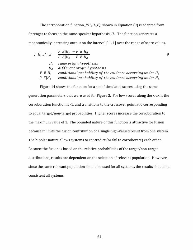
62
The corroboration function, f(Hs,Hd,E), shown in Equation (9) is adapted from
Sprenger to focus on the same-speaker hypothesis, Hs. The function generates a
monotonically increasing output on the interval [-1, 1] over the range of score values.
𝑑𝑑(𝐻𝐻𝑠𝑠,𝐻𝐻𝑑𝑑,𝐸𝐸) =𝑃𝑃(𝐸𝐸|𝐻𝐻𝑠𝑠) − 𝑃𝑃(𝐸𝐸|𝐻𝐻𝑑𝑑)𝑃𝑃(𝐸𝐸|𝐻𝐻𝑠𝑠) + 𝑃𝑃(𝐸𝐸|𝐻𝐻𝑑𝑑)
(9)
𝐻𝐻𝑠𝑠 = 𝑠𝑠𝑠𝑠𝑠𝑠𝑠𝑠 𝑜𝑜𝑜𝑜𝑜𝑜𝑜𝑜𝑜𝑜𝑜𝑜 ℎ𝑦𝑦𝑦𝑦𝑜𝑜𝑦𝑦ℎ𝑠𝑠𝑠𝑠𝑜𝑜𝑠𝑠𝐻𝐻𝑑𝑑 = 𝑑𝑑𝑜𝑜𝑑𝑑𝑑𝑑𝑠𝑠𝑜𝑜𝑠𝑠𝑜𝑜𝑦𝑦 𝑜𝑜𝑜𝑜𝑜𝑜𝑜𝑜𝑜𝑜𝑜𝑜 ℎ𝑦𝑦𝑦𝑦𝑜𝑜𝑦𝑦ℎ𝑠𝑠𝑠𝑠𝑜𝑜𝑠𝑠
𝑃𝑃(𝐸𝐸|𝐻𝐻𝑠𝑠) = 𝑐𝑐𝑜𝑜𝑜𝑜𝑑𝑑𝑜𝑜𝑦𝑦𝑜𝑜𝑜𝑜𝑜𝑜𝑠𝑠𝑐𝑐 𝑦𝑦𝑜𝑜𝑜𝑜𝑝𝑝𝑠𝑠𝑝𝑝𝑜𝑜𝑐𝑐𝑜𝑜𝑦𝑦𝑦𝑦 𝑜𝑜𝑑𝑑 𝑦𝑦ℎ𝑠𝑠 𝑠𝑠𝑒𝑒𝑜𝑜𝑑𝑑𝑠𝑠𝑜𝑜𝑐𝑐𝑠𝑠 𝑜𝑜𝑐𝑐𝑐𝑐𝑜𝑜𝑜𝑜𝑜𝑜𝑜𝑜𝑜𝑜𝑜𝑜 𝑜𝑜𝑜𝑜𝑑𝑑𝑠𝑠𝑜𝑜 𝐻𝐻𝑠𝑠𝑃𝑃(𝐸𝐸|𝐻𝐻𝑑𝑑) = 𝑐𝑐𝑜𝑜𝑜𝑜𝑑𝑑𝑜𝑜𝑦𝑦𝑜𝑜𝑜𝑜𝑜𝑜𝑠𝑠𝑐𝑐 𝑦𝑦𝑜𝑜𝑜𝑜𝑝𝑝𝑠𝑠𝑝𝑝𝑜𝑜𝑐𝑐𝑜𝑜𝑦𝑦𝑦𝑦 𝑜𝑜𝑑𝑑 𝑦𝑦ℎ𝑠𝑠 𝑠𝑠𝑒𝑒𝑜𝑜𝑑𝑑𝑠𝑠𝑜𝑜𝑐𝑐𝑠𝑠 𝑜𝑜𝑐𝑐𝑐𝑐𝑜𝑜𝑜𝑜𝑜𝑜𝑜𝑜𝑜𝑜𝑜𝑜 𝑜𝑜𝑜𝑜𝑑𝑑𝑠𝑠𝑜𝑜 𝐻𝐻𝑑𝑑
Figure 14 shows the function for a set of simulated scores using the same
generation parameters that were used for Figure 3. For low scores along the x-axis, the
corroboration function is -1, and transitions to the crossover point at 0 corresponding
to equal target/non-target probabilities. Higher scores increase the corroboration to
the maximum value of 1. The bounded nature of this function is attractive for fusion
because it limits the fusion contribution of a single high-valued result from one system.
The bipolar nature allows systems to contradict (or fail to corroborate) each other.
Because the fusion is based on the relative probabilities of the target/non-target
distributions, results are dependent on the selection of relevant population. However,
since the same relevant population should be used for all systems, the results should be
consistent all systems.

63
Figure 14. System with good discrimination overlaid with corroboration function.
The results for multiple systems can be combined via a weighted sum, yielding
the corroboration measure, C(Hs,E), shown in Equation (10).
𝐶𝐶(𝐻𝐻𝑠𝑠,𝐸𝐸) = �𝑤𝑤𝑖𝑖 ∙𝑃𝑃(𝐸𝐸|𝐻𝐻𝑠𝑠) − 𝑃𝑃(𝐸𝐸|𝐻𝐻𝑑𝑑)𝑃𝑃(𝐸𝐸|𝐻𝐻𝑠𝑠) + 𝑃𝑃(𝐸𝐸|𝐻𝐻𝑑𝑑)
𝑁𝑁
𝑖𝑖=1
(10)
𝑁𝑁 = 𝑜𝑜𝑜𝑜𝑠𝑠𝑝𝑝𝑠𝑠𝑜𝑜 𝑜𝑜𝑑𝑑 𝑠𝑠𝑦𝑦𝑠𝑠𝑦𝑦𝑠𝑠𝑠𝑠𝑠𝑠 𝑑𝑑𝑜𝑜𝑜𝑜 𝑤𝑤ℎ𝑜𝑜𝑐𝑐ℎ 𝑠𝑠𝑐𝑐𝑜𝑜𝑜𝑜𝑠𝑠𝑠𝑠 𝑤𝑤𝑜𝑜𝑐𝑐𝑐𝑐 𝑝𝑝𝑠𝑠 𝑑𝑑𝑜𝑜𝑠𝑠𝑠𝑠𝑑𝑑 𝑤𝑤𝑖𝑖 = 𝑤𝑤𝑠𝑠𝑜𝑜𝑜𝑜ℎ𝑦𝑦 𝑠𝑠𝑦𝑦𝑦𝑦𝑐𝑐𝑜𝑜𝑠𝑠𝑑𝑑 𝑦𝑦𝑜𝑜 𝑠𝑠𝑠𝑠𝑐𝑐ℎ 𝑦𝑦𝑜𝑜𝑜𝑜𝑐𝑐, 𝑠𝑠𝑜𝑜𝑠𝑠𝑠𝑠𝑜𝑜𝑜𝑜𝑜𝑜 𝑦𝑦𝑜𝑜 1
For simplicity, this paper will use an equal weighting of all systems (e.g. wi=1/N).
For the systems with asymmetric scoring, each direction will receive half of its weight
(e.g. wi=1/2N). More elaborate schemes could be devised to give higher weight to
higher performing systems. For example, a performance metric (e.g. EER, Cdet, Cllr, etc.)
could factor into the weighting, or a system that has been trained with data that is more
similar to case conditions might receive a higher relative weighting.

64
Conclusions
Above all else, the conclusion for an examination should answer the forensic
question established during the Administrative Assessment. The answer must be
scientifically base, but expressed in a manner that the trier of fact. More briefly, the
conclusion must meet the conditions of Rule 702.
Interpreting Results
Automated systems easily product numerical comparison results, either as a raw
score, an LR, or an LLR. Independent of the actual meaning of the number, the value
itself is variable based on the samples being compared, the relevant population selected
for the analysis, the algorithm being used, and the data used to train the algorithm.
Presumably, the value falls in a deterministic range for the system to be at all useful, but
the value nevertheless is variable. For example, the result of comparing the first minute
of a speech sample should be approximately the same as the second minute (assuming
the sample is relatively consistent throughout), but will almost certainly not be
identical. Therefore, a “correct” answer does not exist; and if not, how can examiner
prove that a given answer is the correct one, or even an approximately correct one? (To
paraphrase George Box [65], “All answers are wrong, but some can be useful.”) How
could an examiner defend such an answer to a challenge (in a courtroom or otherwise)?
The debate on the issue of Trial by Mathematics dates back almost fifty years to Tribe
[66] and subsequent commentary [67], [68] and is not likely to be settled any time
soon. The position of this paper, however, is that a verbal scale avoids this issue and
provides an assessment that is more easily communicated to the trier of fact.

65
Converting a numeric, scientifically based result to a verbal scale that is easily
understood by a non-scientific person is a threefold challenge:
• The scientific basis of the original result should be maintained.
• The numeric values must be mapped to verbal descriptions.
• The verbal descriptions must imply a consistent meaning across a variety of
consumers.
One challenge for the FSC community is that some methods (not addressed in
this paper) generate non-numeric results to begin with. However, specific ENFSI
guidelines for speaker recognition [59] say:
Whereas the output of a FASR or FSASR method or a combination thereof allows a numerical strength of evidence statement, this is usually not possible with other methods of FSR coming from the domain of the auditory-phonetic-and-acoustic-phonetic approach. If the results from both domains of FSR are combined, the outcome cannot be a numerical statement since the auditory-phonetic-and-acoustic-phonetic approach cannot provide this. The remaining options are verbal statements. If the outcome of the auditory-phonetic-and-acoustic-phonetic analysis is expressed as verbal statement, the combination with the quantitative LR by the FASR or FSASR system can be achieved verbally.
An additional challenge for the FSC community is that the standard LR or LLR (or
even a raw score) is not a bounded value, so proposed scales have a tendency to
address the lower LR range and ignore the upper range. For example, Table 3 shows a
10-level scale adapted from ENFSI guidelines [69]. Some laboratories (e.g. Nordgaard
[70]) collapse the “limited support” for both hypotheses into an “inconclusive” rating,
yielding a 9-level scale. Other laboratories collapse additional levels into a
corresponding 7-level or 5-level scale.
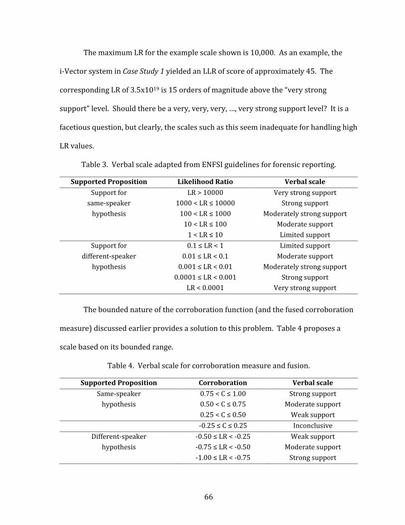
66
The maximum LR for the example scale shown is 10,000. As an example, the
i-Vector system in Case Study 1 yielded an LLR of score of approximately 45. The
corresponding LR of 3.5x10¹⁹ is 15 orders of magnitude above the “very strong
support” level. Should there be a very, very, very, …, very strong support level? It is a
facetious question, but clearly, the scales such as this seem inadequate for handling high
LR values.
Table 3. Verbal scale adapted from ENFSI guidelines for forensic reporting.
Supported Proposition Likelihood Ratio Verbal scale Support for LR > 10000 Very strong support
same-speaker 1000 < LR ≤ 10000 Strong support hypothesis 100 < LR ≤ 1000 Moderately strong support
10 < LR ≤ 100 Moderate support 1 < LR ≤ 10 Limited support
Support for 0.1 ≤ LR < 1 Limited support different-speaker 0.01 ≤ LR < 0.1 Moderate support
hypothesis 0.001 ≤ LR < 0.01 Moderately strong support 0.0001 ≤ LR < 0.001 Strong support LR < 0.0001 Very strong support
The bounded nature of the corroboration function (and the fused corroboration
measure) discussed earlier provides a solution to this problem. Table 4 proposes a
scale based on its bounded range.
Table 4. Verbal scale for corroboration measure and fusion.
Supported Proposition Corroboration Verbal scale Same-speaker 0.75 < C ≤ 1.00 Strong support
hypothesis 0.50 < C ≤ 0.75 Moderate support 0.25 < C ≤ 0.50 Weak support -0.25 ≤ C ≤ 0.25 Inconclusive
Different-speaker -0.50 ≤ LR < -0.25 Weak support hypothesis -0.75 ≤ LR < -0.50 Moderate support
-1.00 ≤ LR < -0.75 Strong support
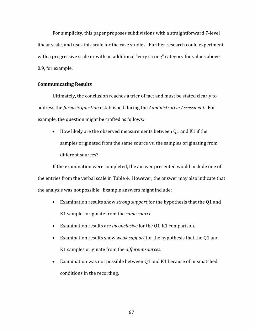
67
For simplicity, this paper proposes subdivisions with a straightforward 7-level
linear scale, and uses this scale for the case studies. Further research could experiment
with a progressive scale or with an additional “very strong” category for values above
0.9, for example.
Communicating Results
Ultimately, the conclusion reaches a trier of fact and must be stated clearly to
address the forensic question established during the Administrative Assessment. For
example, the question might be crafted as follows:
• How likely are the observed measurements between Q1 and K1 if the
samples originated from the same source vs. the samples originating from
different sources?
If the examination were completed, the answer presented would include one of
the entries from the verbal scale in Table 4. However, the answer may also indicate that
the analysis was not possible. Example answers might include:
• Examination results show strong support for the hypothesis that the Q1 and
K1 samples originate from the same source.
• Examination results are inconclusive for the Q1-K1 comparison.
• Examination results show weak support for the hypothesis that the Q1 and
K1 samples originate from the different sources.
• Examination was not possible between Q1 and K1 because of mismatched
conditions in the recording.
68
Case Studies
The case studies presented in the following sections were developed using voice
samples from a data set compiled by the Federal Bureau of Investigation (FBI) Forensic
Audio, Video, and Image Analysis Unit (FAVIAU). The data set comprises fourteen
conditions based on data assembled from other collections. Each condition contains
two samples each for a number of speakers, organized into two sessions according to
common characteristics. Condition Set 3, for example, consists of data from two
different source collections, all male voice samples recorded with a studio-quality
microphone. Session 1 of the set contains English recordings, and session 2 contains a
mixture of three other languages (Spanish, Arabic, and Korean). Other condition sets
use data from other collections, microphone types, languages, or communication
channels. Each condition set thus forms a relevant population for the conditions under
which it was assembled.
The voice samples are annotated as to the originating speaker, so the ground
truth is presumably known for each sample. However, in assembling such an extensive
corpus of data, occasional errors creep in. Therefore, the truth-marking provided was
taken as a strong hint of the originating speaker rather than as absolute knowledge.
The data was received as digital recordings (.wav) on DVD media, and message digests
were computed for each sample. The evidence handling portion of the framework, then,
was conducted identically across all case studies and according to best practices, and
will not be discussed in detail for each case. Similarly, the case studies will assume the
availability of data resources, and examiner qualifications in the Case Assessment

69
section, and issues related to independent verification and administrative review will
not be included in the discussion.
During the analysis phase, four speaker recognition systems were used, each
implementing a different algorithm:
• GMM-UBM – A system using Gaussian Mixture Models and a Universal
Background Model that models the statistics of the acoustic properties in the
voice samples (Reynolds [71]).
• SVM – A system using a Support Vector Machine to discriminate acoustic
properties of voice samples in high dimensional space (Campbell [72])
• i-Vector – A system that models the variability in voice samples and
compares similarity across models (Kenney [73])
• DNN – An i-Vector system combined with a Deep Neural Network trained to
recognize voice samples enrolled in the system (Richardson [74])
The case studies demonstrate the framework described above through a series
of increasingly complex conditions. Because of the way the GMM-UBM and SVM
algorithms function, those systems produce raw scores (i.e. not likelihood ratios) that
are asymmetric under reverse testing conditions. That is, testing sample A against a
model built from sample B will generate a different score than testing sample B against
a model built from sample A. The i-Vector and DNN systems produce log-likelihood
ratios (LLRs) that are symmetric under reverse testing. Case Study 1 will illustrate this
point in the generated plots, and the remaining case studies will not show the
duplicates explicitly.

70
Case Study 1
In this case, samples from the same speaker were selected from Condition Set 4.
Both sessions for this condition are taken from the NIST’99 corpus and consist of 225
male speakers speaking English over a landline telephone.
Case 1 Forensic Request
This case involves a one-to-one comparison of a questioned voice sample (Q1)
against a known sample (K1) to determine if they originated from the same speaker.
The case evidence is summarized in Table 5.
Table 5. Case 1 evidence files.
Questioned Samples Known Samples Label: Q1 K1 File Name: N9_1106~0000_M_Tk_Eng_S1.wav N9_1106~0000_M_Tk_Eng_S2.wav Language: English English Source Device: Landline telephone Landline telephone
Case 1 Assessment
Initial assessment revealed no issues with the specified language, file format, or
source device for the data. The data was in digital format, so no analog conversion or
other processing was required. Auditory analysis of the Q1 recording revealed the
following subjective observations:
• Solo male speaker, speaking English.
• Restricted signal bandwidth consistent with a telephone channel.
• Minor codec effects.
• Occasional distortion on plosive sounds, presumably to microphone
proximity.
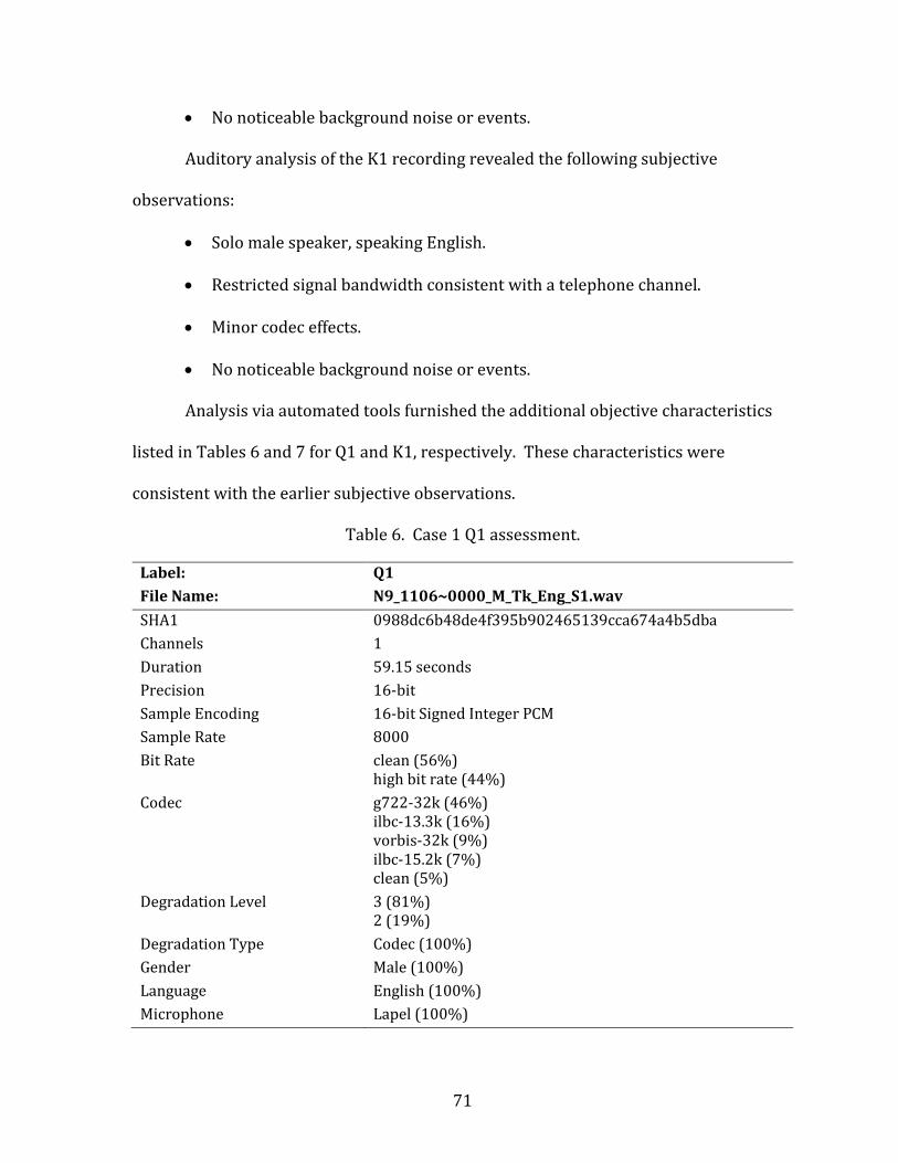
71
• No noticeable background noise or events.
Auditory analysis of the K1 recording revealed the following subjective
observations:
• Solo male speaker, speaking English.
• Restricted signal bandwidth consistent with a telephone channel.
• Minor codec effects.
• No noticeable background noise or events.
Analysis via automated tools furnished the additional objective characteristics
listed in Tables 6 and 7 for Q1 and K1, respectively. These characteristics were
consistent with the earlier subjective observations.
Table 6. Case 1 Q1 assessment.
Label: Q1 File Name: N9_1106~0000_M_Tk_Eng_S1.wav SHA1 0988dc6b48de4f395b902465139cca674a4b5dba Channels 1 Duration 59.15 seconds Precision 16-bit Sample Encoding 16-bit Signed Integer PCM Sample Rate 8000 Bit Rate clean (56%)
high bit rate (44%) Codec g722-32k (46%)
ilbc-13.3k (16%) vorbis-32k (9%) ilbc-15.2k (7%) clean (5%)
Degradation Level 3 (81%) 2 (19%)
Degradation Type Codec (100%) Gender Male (100%) Language English (100%) Microphone Lapel (100%)

72
Table 7. Case 1 K1 assessment.
Label: K1 File Name: N9_1106~0000_M_Tk_Eng_S2.wav SHA1 43952f8f7c20009d78afd7ce72ca3130f08723e6 Channels 1 Duration 60.3 seconds Precision 16-bit Sample Encoding 16-bit Signed Integer PCM Sample Rate 8000 Bit Rate clean (57%)
high bit rate (39%) medium bit rate (4%)
Codec ilbc-13.3k (22%) aac-32k (17%) g711-64k (9%) mp3-64k (9%) vorbis-32k (9%) clean (9%) aac-64k (7%) opus-vbr-16k (6%) ilbc-15.2k (4%) g722-32k (3%) opus-16k (2%)
Degradation Level 0 (100%) Degradation Type Codec (100%) Degradation Level 0 (100%) Gender Male (100%) Language English (100%) Microphone Lapel (100%)
The significant extrinsic mismatch conditions include codec effects and the
plosive distortion. No significant intrinsic mismatch conditions were discerned. The
automated tools correctly detected the English language. Additionally, the moderate
degradation level (3 on a scale of 0 to 4) for one of the samples should cause the
examiner to consider the degradation in evaluating the results obtained from the
systems. The duration and quality of the samples were deemed appropriate for
processing with the available tools.
73
Forensic Question:
• How likely are the observed measurements between Q1 and K1 if the
samples originated from the same source vs. the samples originating from
different sources?
Case 1 Analysis and Processing
No additional data preparation or enhancement was required, and the data in
the Condition Set 4 data set was judged appropriate as a relevant population. The Q1
and K1 samples were submitted to the four algorithms, with the resulting plots shown
in Figures 15 through 34.
For the GMM-UBM algorithm, Figure 15 shows the target/non-target score
distributions from testing the session 1 samples against the session 2 models (1v2),
with the vertical line corresponding to the score of Q1 (which originated from session
1) against a model built from K1 (which originated from session 2). Figure 17 shows
session 2 against session 1 (2v1), with the vertical line corresponding to the score of K1
against a model built from Q1. The high scores in both comparisons support the same-
speaker hypothesis.
The DET plots in Figures 16 and 18 show a generally linear curve except for the
edges where a limited number of trial errors (Doddington’s Rule of 30) cause the plot to
lose resolution. The equal error rate (EER) for this algorithm under the given data
conditions is approximately 3%. Figure 19 shows the results of the 1v2 and 2v1 tests
for the top ten similarity scores in the other session of the relevant population. For
both test directions, Q1 and K1 show the highest similarity to each other.

74
Figures 20 through 24 show the results for the SVM algorithm. The plots show
that the system exhibits less overall discrimination than the GMM-UBM system, with an
EER of about 6%. The scores in both directions support the same-speaker hypothesis.
The i-Vector results in Figures 25 through 29 and the DNN results in Figures 30
through 34 show comparable results to the previous algorithms. Since they use
symmetric scoring, Figures 25, 26, 30, and 31 are identical to Figures 27, 28, 32, and 33,
respectively. However, Figures 29 and 34 are not identical because the scores shown
are the top ten results in the other session. The DET plots illustrate the improved
discrimination for these more modern algorithms, with EERs of approximately 1% on
this data set. The lower EERs result in low resolution of the DET curve extending into
the center of the plot. This example illustrates a paradox in assessing speaker
recognition algorithms, as the more accurate the systems become (i.e. the fewer errors
they make), the more difficult the evaluation of the system becomes.
The astute reader also will notice that the score axis on the score distribution
plots scales differently among the different systems because of the differences in
operation.
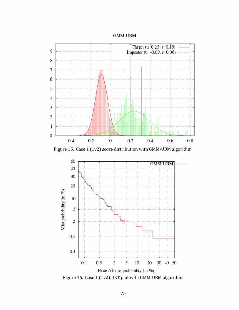
75
Figure 15. Case 1 (1v2) score distribution with GMM-UBM algorithm.
Figure 16. Case 1 (1v2) DET plot with GMM-UBM algorithm.

76
Figure 17. Case 1 (2v1) score distribution with GMM-UBM algorithm.
Figure 18. Case 1 (2v1) DET plot with GMM-UBM algorithm.

77
Figure 19. Case 1 (1v2 and 2v1) score ranking with GMM-UBM algorithm.
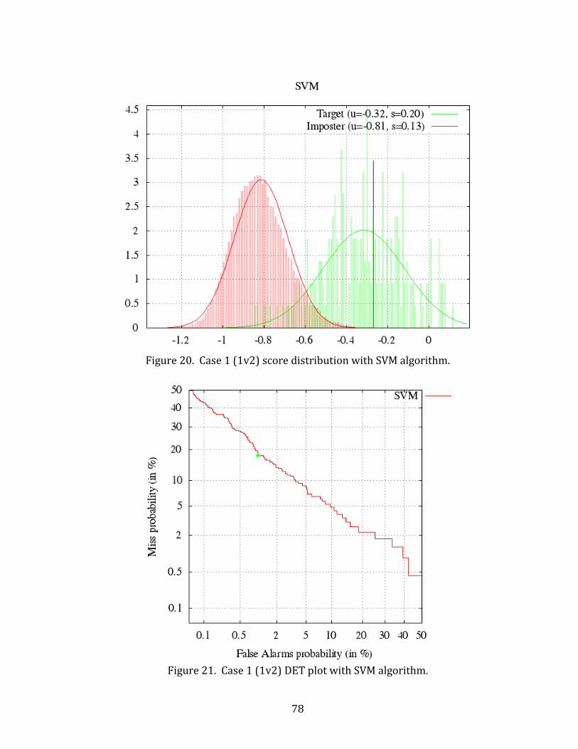
78
Figure 20. Case 1 (1v2) score distribution with SVM algorithm.
Figure 21. Case 1 (1v2) DET plot with SVM algorithm.

79
Figure 22. Case 1 (2v1) score distribution with SVM algorithm.
Figure 23. Case 1 (2v1) DET plot with SVM algorithm.
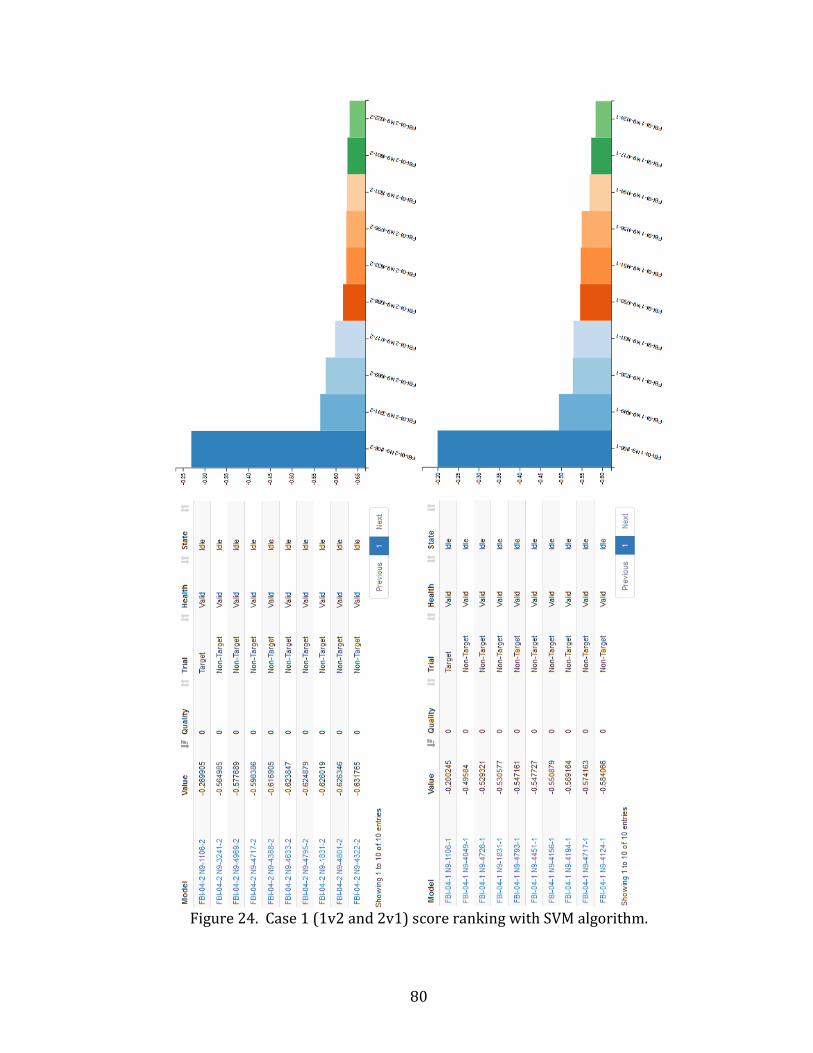
80
Figure 24. Case 1 (1v2 and 2v1) score ranking with SVM algorithm.

81
Figure 25. Case 1 (1v2) score distribution with i-Vector algorithm.
Figure 26. Case 1 (1v2) DET plot with i-Vector algorithm.

82
Figure 27. Case 1 (2v1) score distribution with i-Vector algorithm.
Figure 28. Case 1 (2v1) DET plot with i-Vector algorithm.

83
Figure 29. Case 1 (1v2 and 2v1) score ranking with i-Vector algorithm.

84
Figure 30. Case 1 (1v2) score distribution with DNN algorithm.
Figure 31. Case 1 (1v2) DET plot with DNN algorithm.
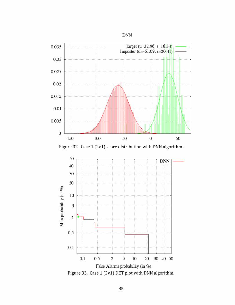
85
Figure 32. Case 1 (2v1) score distribution with DNN algorithm.
Figure 33. Case 1 (2v1) DET plot with DNN algorithm.

86
Figure 34. Case 1 (1v2 and 2v1) score ranking with DNN algorithm.
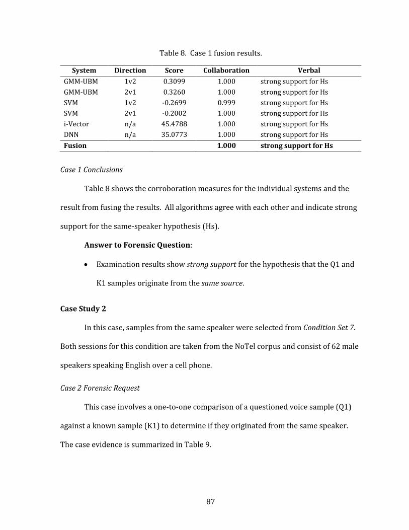
87
Table 8. Case 1 fusion results.
System Direction Score Collaboration Verbal GMM-UBM 1v2 0.3099 1.000 strong support for Hs GMM-UBM 2v1 0.3260 1.000 strong support for Hs SVM 1v2 -0.2699 0.999 strong support for Hs SVM 2v1 -0.2002 1.000 strong support for Hs i-Vector n/a 45.4788 1.000 strong support for Hs DNN n/a 35.0773 1.000 strong support for Hs Fusion 1.000 strong support for Hs
Case 1 Conclusions
Table 8 shows the corroboration measures for the individual systems and the
result from fusing the results. All algorithms agree with each other and indicate strong
support for the same-speaker hypothesis (Hs).
Answer to Forensic Question:
• Examination results show strong support for the hypothesis that the Q1 and
K1 samples originate from the same source.
Case Study 2
In this case, samples from the same speaker were selected from Condition Set 7.
Both sessions for this condition are taken from the NoTel corpus and consist of 62 male
speakers speaking English over a cell phone.
Case 2 Forensic Request
This case involves a one-to-one comparison of a questioned voice sample (Q1)
against a known sample (K1) to determine if they originated from the same speaker.
The case evidence is summarized in Table 9.
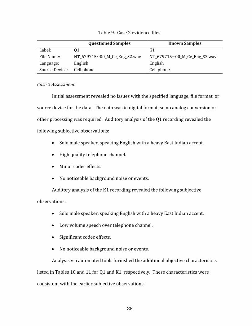
88
Table 9. Case 2 evidence files.
Questioned Samples Known Samples Label: Q1 K1 File Name: NT_679715~00_M_Ce_Eng_S2.wav NT_679715~00_M_Ce_Eng_S3.wav Language: English English Source Device: Cell phone Cell phone
Case 2 Assessment
Initial assessment revealed no issues with the specified language, file format, or
source device for the data. The data was in digital format, so no analog conversion or
other processing was required. Auditory analysis of the Q1 recording revealed the
following subjective observations:
• Solo male speaker, speaking English with a heavy East Indian accent.
• High quality telephone channel.
• Minor codec effects.
• No noticeable background noise or events.
Auditory analysis of the K1 recording revealed the following subjective
observations:
• Solo male speaker, speaking English with a heavy East Indian accent.
• Low volume speech over telephone channel.
• Significant codec effects.
• No noticeable background noise or events.
Analysis via automated tools furnished the additional objective characteristics
listed in Tables 10 and 11 for Q1 and K1, respectively. These characteristics were
consistent with the earlier subjective observations.

89
Table 10. Case 2 Q1 assessment.
Label: Q1 File Name: NT_679715~00_M_Ce_Eng_S2.wav SHA1 743e6216c23253d79614fb3ef77017e14f4cffca Channels 1 Duration 54.48 seconds Precision 16-bit Sample Encoding 16-bit Signed Integer PCM Sample Rate 8000 Bit Rate clean (100%) Codec clean (66%)
amrnb-12.2k (17%) opus-vbr-4k (7%) opus-vbr-8k (5%)
Degradation Level 4 (100%) Degradation Type Codec (100%) Gender Male (82%)
Female (18%) Language Unknown (100%) Microphone video (98%)
Table 11. Case 2 K1 assessment.
Label: K1 File Name: NT_679715~00_M_Ce_Eng_S3.wav SHA1 a9179bf599e945b1912aee996de89c820947bb22 Channels 1 Duration 54.49 seconds Precision 16-bit Sample Encoding 16-bit Signed Integer PCM Sample Rate 8000 Bit Rate clean (100%) Codec amrnb-5.9k (62%)
clean (10%) ilbc-13.3k (19%) ilbc-15.2k (3%) opus-vbr-4k (3%)
Degradation Level 4 (100%) Degradation Type Codec (100%) Gender Male (99%) Language Unknown (100%)

90
Microphone phone (100%)
The extrinsic mismatch conditions include codec effects and a significant volume
difference (which may have an effect on the influence of the codec effects).
Additionally, the high degradation level (4 on a scale of 0 to 4) for the samples may
predict a lower reliability in the systems. No significant intrinsic mismatch conditions
were discerned, but the automated tools were unable to detect the English language
being spoken. (The issue of processing English with a heavy East Indian accent is a
known one, and occurred during the 2006 SRE. To speaker recognition algorithms, this
speech “looks” like a completely different language from English.) The duration and
quality of the samples were deemed appropriate for processing with the available tools.
Forensic Question:
• How likely are the observed measurements between Q1 and K1 if the
samples originated from the same source vs. the samples originating from
different sources?
Case 2 Analysis and Processing
No additional data preparation or enhancement was required, and the data in
the Condition Set 7 data set was judged appropriate as a relevant population. The Q1
and K1 samples were submitted to the four algorithms, with the resulting plots shown
in Figures 35 through 50.
The plots for the GMM-UBM algorithm in Figures 35 through 39 reveal a lower
discriminative capability for this data set. Further, the score distributions are deviating
from the expected Gaussian envelope. The target scores are somewhat scattered, and
the non-target distributions show a narrowed distribution with a positive skew.
91
Additionally, the limited data set (62 speakers in each session) results in a lower
resolution DET plot, with the EER exceeding 10%. The score ranking in Figure 39
shows disagreement between the 1v2 and 2v1 tests. The score for the 1v2 test is
mostly in the target region in Figure 35 but still on the edge of the non-target area.
However, in the score ranking it still shows the highest similarity with its truth-marked
companion in the other session. The 2v1 test shows to be firmly established in the
target region, but the score ranking shows two other speakers ranked with higher
similarity than its truth-marked companion. This situation demonstrates the value of
reverse testing to detect if a particular algorithm is having difficulty dealing with
mismatched conditions or low-quality data.
The SVM plots in Figures 40 through 44 reveal similar discrimination
performance as the GMM-UBM system, with an EER also above 10%. As for the GMM-
UBM algorithm the score for the 2v1 test appears more confident than the 1v2, but for
this algorithm, the score ranking successfully shows the highest similarity with its
truth-marked companion for both tests (but for the 1v2 test, just barely).
The i-Vector and DNN results in Figures 45 through 50 are even more
interesting. The non-target score distributions show deviations from the expected
Gaussian envelope, and the DET plots are starting to look more rounded, similar to the
plots using simulated scores with a triangular distribution in the section, System with
Unrealistic Data. The results from the i-Vector algorithm tends toward the different
speaker hypothesis, but the equivalent result from the DNN algorithm shows the
opposite same speaker.hypothesis tendency. This situation demonstrates the value of
using different algorithms for cross-validation.
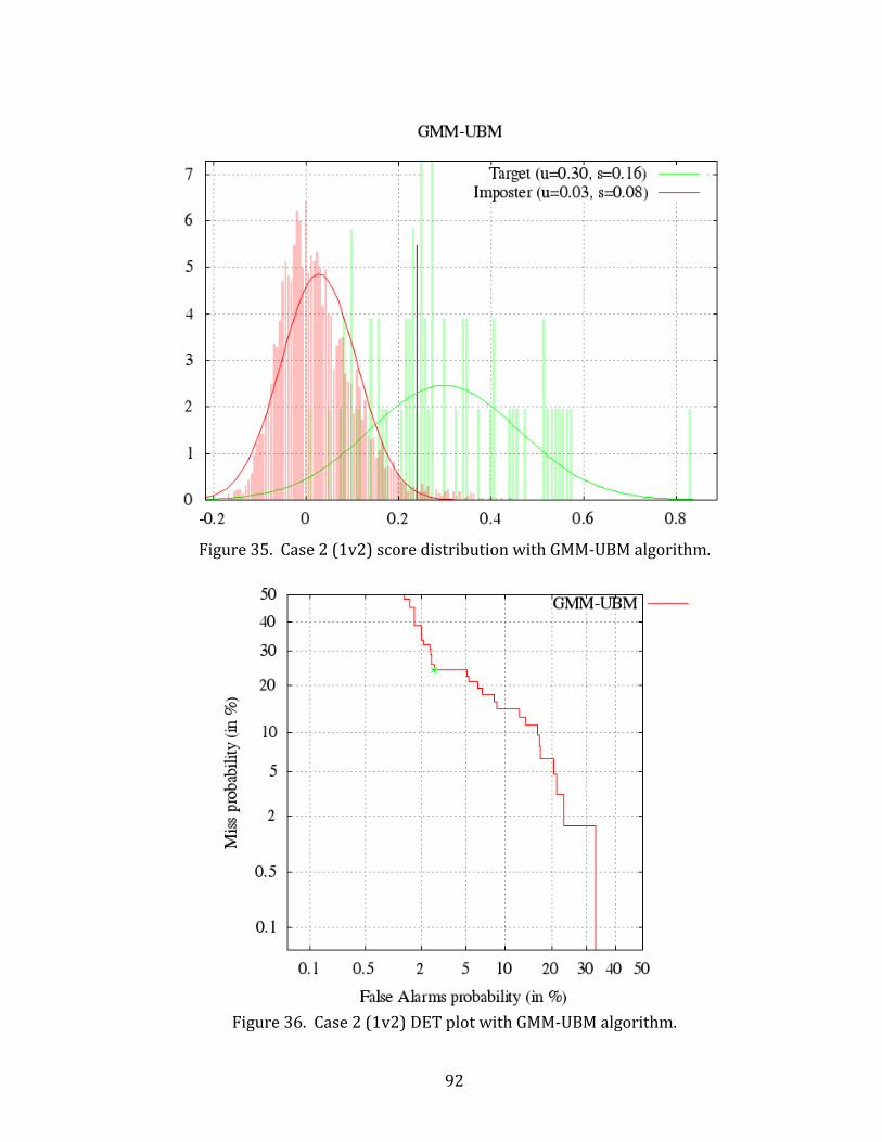
92
Figure 35. Case 2 (1v2) score distribution with GMM-UBM algorithm.
Figure 36. Case 2 (1v2) DET plot with GMM-UBM algorithm.

93
Figure 37. Case 2 (2v1) score distribution with GMM-UBM algorithm.
Figure 38. Case 2 (2v1) DET plot with GMM-UBM algorithm.

94
Figure 39. Case 2 (1v2 and 2v1) score ranking with GMM-UBM algorithm.
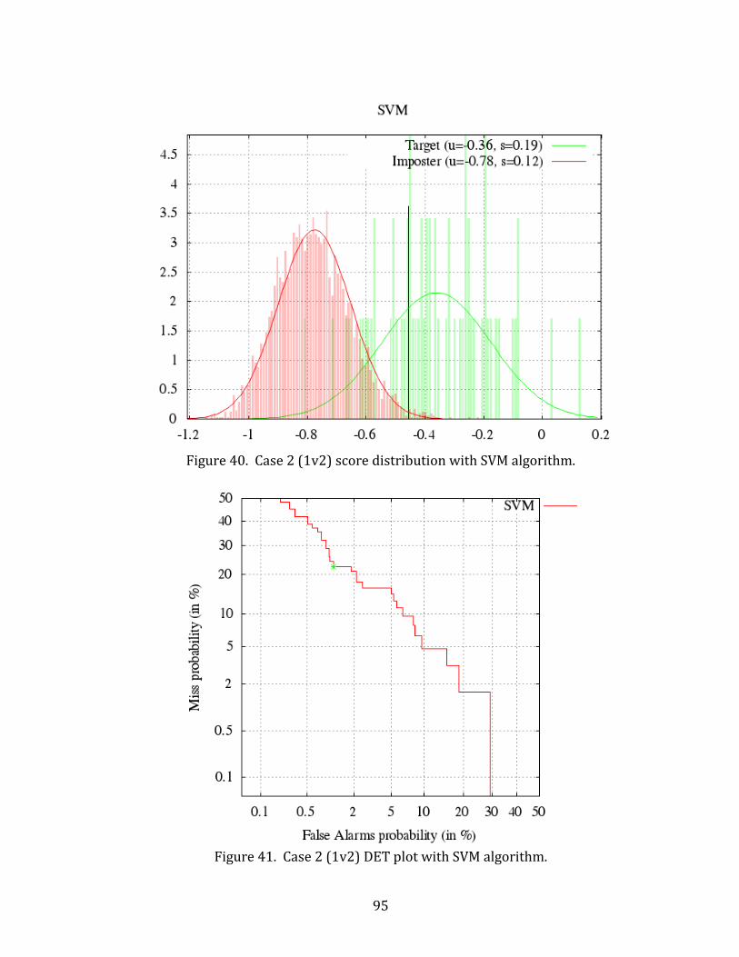
95
Figure 40. Case 2 (1v2) score distribution with SVM algorithm.
Figure 41. Case 2 (1v2) DET plot with SVM algorithm.

96
Figure 42. Case 2 (2v1) score distribution with SVM algorithm.
Figure 43. Case 2 (2v1) DET plot with SVM algorithm.

97
Figure 44. Case 2 (1v2 and 2v1) score ranking with SVM algorithm.

98
Figure 45. Case 2 (1v2 or 2v1) score distribution with i-Vector algorithm.
Figure 46. Case 2 (1v2 or 2v1) DET plot with i-Vector algorithm.
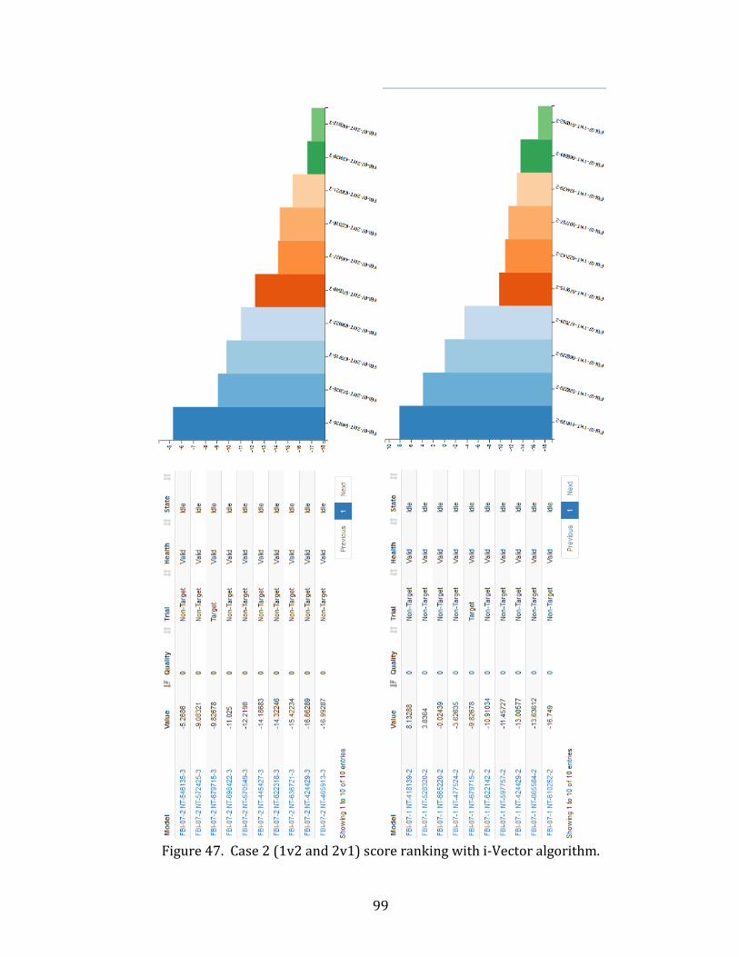
99
Figure 47. Case 2 (1v2 and 2v1) score ranking with i-Vector algorithm.

100
Figure 48. Case 2 (1v2 or 2v1) score distribution with DNN algorithm.
Figure 49. Case 2 (1v2 or 2v1) DET plot with DNN algorithm.

101
Figure 50. Case 2 (1v2 and 2v1) score ranking with DNN algorithm.

102
Table 12. Case 2 fusion results.
System Direction Score Collaboration Verbal GMM-UBM 1v2 0.2386 0.866 strong support for Hs GMM-UBM 2v1 0.3164 0.993 strong support for Hs SVM 1v2 -0.4550 0.912 strong support for Hs SVM 2v1 -0.3101 0.995 strong support for Hs i-Vector n/a -9.8268 -0.670 moderate support for Hd DNN n/a 20.8858 0.886 strong support for Hs Fusion 0.525 moderate support for Hs
Case 2 Conclusions
Table 12 shows the corroboration measures for the individual systems and the
result from fusing the results. All but the i-Vector algorithm agree with each other, but
the fused result indicate moderate support for the same-speaker hypothesis (Hs).
Answer to Forensic Question:
• Examination results show moderate support for the hypothesis that the Q1
and K1 samples originate from the same source.
Case Study 3
In this case, samples from the same speaker were selected from Condition Set 6.
The sessions for this condition are taken from both the Bilingual and CrossInt corpora
and consist of 597 male speakers speaking English vs. non-English over a landline
telephone. Session one includes samples in which the speaker is speaking English,
while session two includes samples in Arabic, Bengali, Hindi, Kannada, Punjabi,
Malayalam, Marathi, Tamil, Korean, and Spanish.

103
Case 3 Forensic Request
This case involves a one-to-one comparison of a questioned voice sample (Q1)
against a known sample (K1) to determine if they originated from the same speaker.
The case evidence is summarized in Table 13.
Table 13. Case 3 evidence files.
Questioned Samples Known Samples Label: Q1 K1 File Name: CI_0797~0000_M_Tk_Eng_S1.wav CI_0797~0000_M_Tk_Tam_S2.wav Language: English Tamil Source Device: Landline telephone Landline telephone
Case 3 Assessment
Initial assessment revealed no issues with the specified language, file format, or
source device for the data. The data was in digital format, so no analog conversion or
other processing was required. Auditory analysis of the Q1 recording revealed the
following subjective observations:
• Solo male speaker, speaking English with a heavy accent similar to an East
Indian accent, but different.
• Slightly elevated voice pitch.
• High quality telephone channel.
• Minor codec effects.
• No noticeable background noise or events.
Auditory analysis of the K1 recording revealed the following subjective
observations:
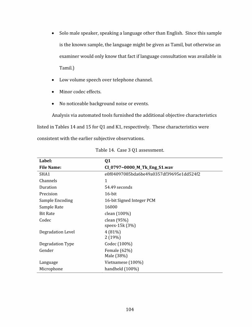
104
• Solo male speaker, speaking a language other than English. Since this sample
is the known sample, the language might be given as Tamil, but otherwise an
examiner would only know that fact if language consultation was available in
Tamil.)
• Low volume speech over telephone channel.
• Minor codec effects.
• No noticeable background noise or events.
Analysis via automated tools furnished the additional objective characteristics
listed in Tables 14 and 15 for Q1 and K1, respectively. These characteristics were
consistent with the earlier subjective observations.
Table 14. Case 3 Q1 assessment.
Label: Q1 File Name: CI_0797~0000_M_Tk_Eng_S1.wav SHA1 e0f04097085bda6be49a0357df39695e1dd524f2 Channels 1 Duration 54.49 seconds Precision 16-bit Sample Encoding 16-bit Signed Integer PCM Sample Rate 16000 Bit Rate clean (100%) Codec clean (95%)
speex-15k (3%) Degradation Level 4 (81%)
2 (19%) Degradation Type Codec (100%) Gender Female (62%)
Male (38%) Language Vietnamese (100%) Microphone handheld (100%)
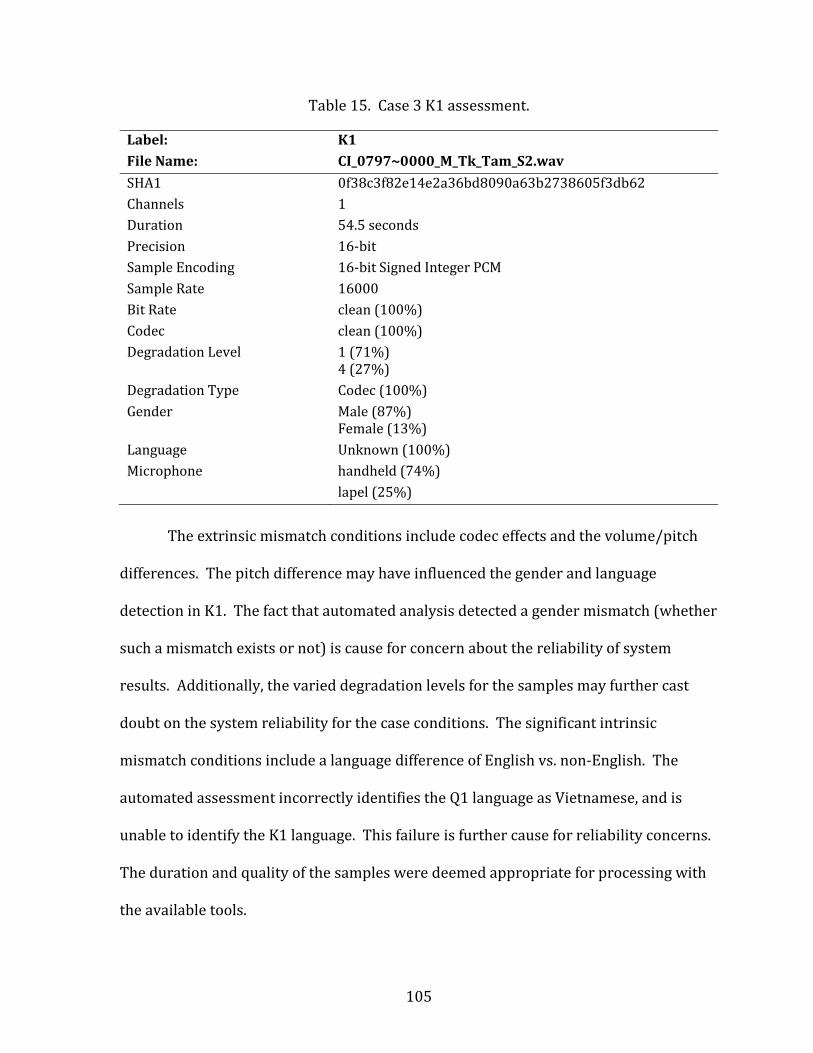
105
Table 15. Case 3 K1 assessment.
Label: K1 File Name: CI_0797~0000_M_Tk_Tam_S2.wav SHA1 0f38c3f82e14e2a36bd8090a63b2738605f3db62 Channels 1 Duration 54.5 seconds Precision 16-bit Sample Encoding 16-bit Signed Integer PCM Sample Rate 16000 Bit Rate clean (100%) Codec clean (100%) Degradation Level 1 (71%)
4 (27%) Degradation Type Codec (100%) Gender Male (87%)
Female (13%) Language Unknown (100%) Microphone handheld (74%)
lapel (25%)
The extrinsic mismatch conditions include codec effects and the volume/pitch
differences. The pitch difference may have influenced the gender and language
detection in K1. The fact that automated analysis detected a gender mismatch (whether
such a mismatch exists or not) is cause for concern about the reliability of system
results. Additionally, the varied degradation levels for the samples may further cast
doubt on the system reliability for the case conditions. The significant intrinsic
mismatch conditions include a language difference of English vs. non-English. The
automated assessment incorrectly identifies the Q1 language as Vietnamese, and is
unable to identify the K1 language. This failure is further cause for reliability concerns.
The duration and quality of the samples were deemed appropriate for processing with
the available tools.

106
Forensic Question:
• How likely are the observed measurements between Q1 and K1 if the
samples originated from the same source vs. the samples originating from
different sources?
Case 3 Analysis and Processing
No additional data preparation or enhancement was required, and the data in
the Condition Set 6 data set was judged appropriate as a relevant population. The Q1
and K1 samples were submitted to the four algorithms, with the resulting plots shown
in Figures 51 through 66.
The plots for the GMM-UBM algorithm in Figures 51 through 55 reveal a lower
discriminative capability for this data set with an EER of about 6% for both the 1v2 and
2v1 test directions. The score distributions are approximately Gaussian, but are slightly
narrowed. The relatively large number of samples in the relevant population generate
good statistics for the case, and the DET plot is relatively linear with good resolution.
Despite the truth marking, however, the system clearly shows low similarity between
Q1 and K1, and the truth-marked companion for both sessions does not even appear in
the top ten list of similar scores in either the 1v2 or 2v1 test directions. This algorithm
clearly detects little similarity between Q1 and K1.
The SVM plots in Figures 56 through 60 reveal lower discrimination
performance than the GMM-UBM system, with an EER approximately 9%. The non-
target distribution indicates a slightly positive skew. The scores are more strongly in
the non-target distribution, and the truth-marked companion for both sessions is
107
absent from the top ten list. This algorithm also detects little similarity between Q1 and
K1.
The i-Vector and DNN results in Figures 61 through 66 show non-target
distributions with a slightly negative skew, and the DET plots show an EER of
approximately 4%. The i-Vector DET plot exhibits a nonlinearity at higher false alarm
rates. The scores are noticeably in the target distribution area, but, the score ranking
disturbingly shows the truth-marked companions not to be the highest scores.
Therefore, the high similarity assessment by the algorithm is a bit suspect, as the
similarity may originate from features other than the speaker characteristics.
Since the Condition Set 6 relevant population included multiple languages in
session 2, the analysis was repeated using only the six Tamil language samples from the
session. Figures 67 through 78 show the equivalent plots. The scoring results are
essentially unchanged, and the sparseness of the plots show the inadequate statistics
for proper assessment.
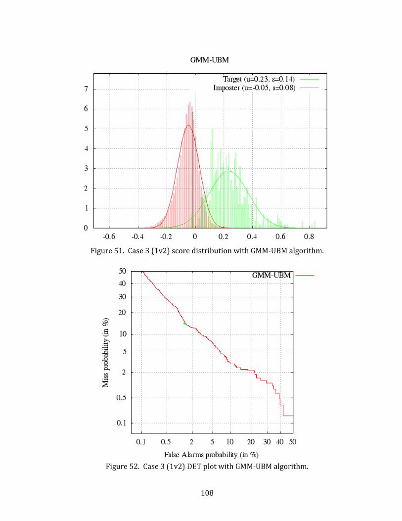
108
Figure 51. Case 3 (1v2) score distribution with GMM-UBM algorithm.
Figure 52. Case 3 (1v2) DET plot with GMM-UBM algorithm.

109
Figure 53. Case 3 (2v1) score distribution with GMM-UBM algorithm.
Figure 54. Case 3 (2v1) DET plot with GMM-UBM algorithm.

110
Figure 55. Case 3 (1v2 and 2v1) score ranking with GMM-UBM algorithm.
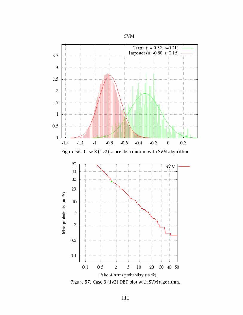
111
Figure 56. Case 3 (1v2) score distribution with SVM algorithm.
Figure 57. Case 3 (1v2) DET plot with SVM algorithm.
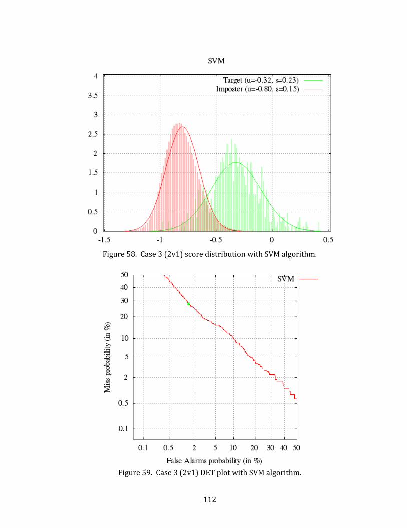
112
Figure 58. Case 3 (2v1) score distribution with SVM algorithm.
Figure 59. Case 3 (2v1) DET plot with SVM algorithm.

113
Figure 60. Case 3 (1v2 and 2v1) score ranking with SVM algorithm.
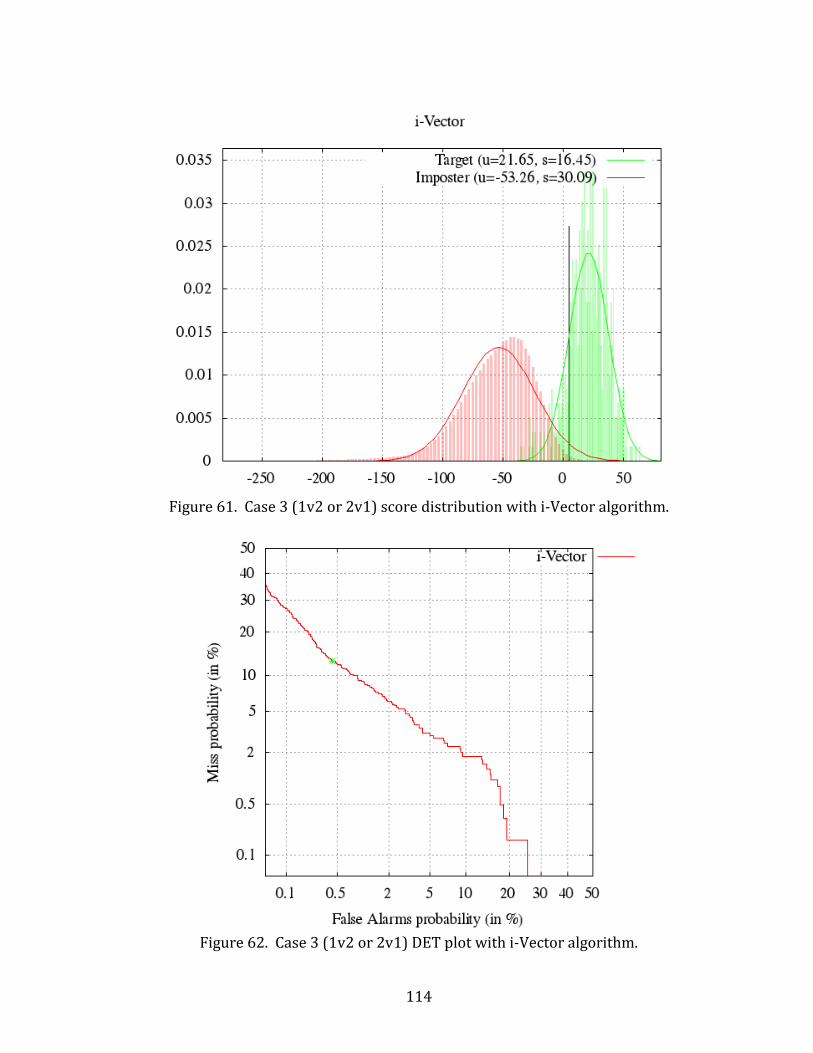
114
Figure 61. Case 3 (1v2 or 2v1) score distribution with i-Vector algorithm.
Figure 62. Case 3 (1v2 or 2v1) DET plot with i-Vector algorithm.

115
Figure 63. Case 3 (1v2 and 2v1) score ranking with i-Vector algorithm.

116
Figure 64. Case 3 (1v2 or 2v1) score distribution with DNN algorithm.
Figure 65. Case 3 (1v2 or 2v1) DET plot with DNN algorithm.
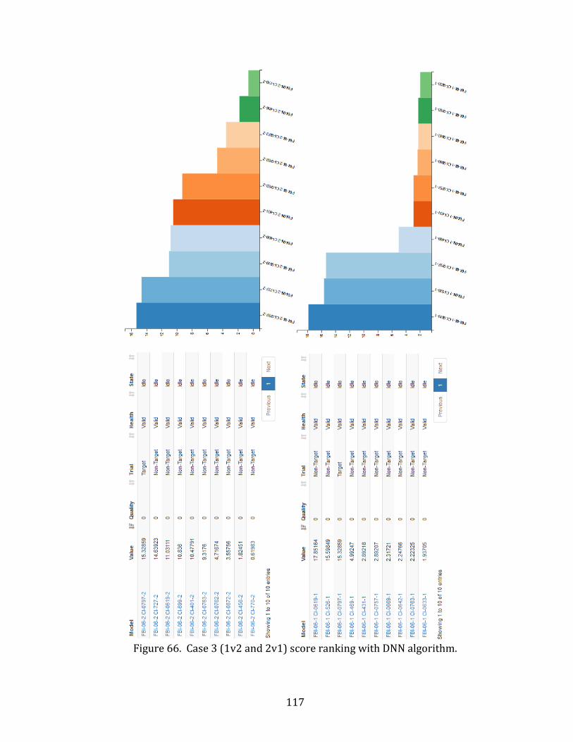
117
Figure 66. Case 3 (1v2 and 2v1) score ranking with DNN algorithm.

118
Figure 67. Case 3 (1v2) with GMM-UBM algorithm using Tamil relevant population.
Figure 68. Case 3 (1v2) DET plot with GMM-UBM using Tamil relevant population.

119
Figure 69. Case 3 (2v1) with GMM-UBM algorithm using Tamil relevant population.
Figure 70. Case 3 (2v1) DET plot with GMM-UBM using Tamil relevant population.

120
Figure 71. Case 3 (1v2) with SVM algorithm using Tamil relevant population.
Figure 72. Case 3 (1v2) DET plot with SVM using Tamil relevant population.
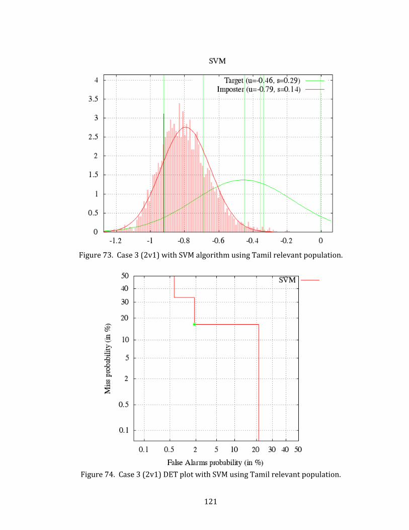
121
Figure 73. Case 3 (2v1) with SVM algorithm using Tamil relevant population.
Figure 74. Case 3 (2v1) DET plot with SVM using Tamil relevant population.

122
Figure 75. Case 3 (1v2 or 2v1) with i-Vector algorithm using Tamil relevant population.
Figure 76. Case 3 (1v2 or 2v1) DET plot with i-Vector using Tamil relevant population.

123
Figure 77. Case 3 (1v2 or 2v1) with DNN algorithm using Tamil relevant population.
Figure 78. Case 3 (1v2 or 2v1) DET plot with DNN using Tamil relevant population.

124
Table 16. Case 3 fusion results.
System Direction Score Collaboration Verbal GMM-UBM 1v2 -0.0183 -0.773 strong support for Hd GMM-UBM 2v1 -0.0330 -0.818 strong support for Hd SVM 1v2 -0.9053 -0.963 strong support for Hd SVM 2v1 -0.9218 -0.943 strong support for Hd i-Vector n/a 4.9872 0.754 strong support for Hs DNN n/a 15.3286 0.864 strong support for Hs Fusion -0.032 inconclusive
Table 17. Case 3 fusion results using Tamil relevant population.
System Direction Score Collaboration Verbal GMM-UBM 1v2 -0.0183 -0.763 strong support for Hd GMM-UBM 2v1 -0.0330 -0.683 moderate support for Hd SVM 1v2 -0.9053 -0.711 moderate support for Hd SVM 2v1 -0.9218 -0.651 moderate support for Hd i-Vector n/a 4.9872 0.860 strong support for Hs DNN n/a 15.3286 0.925 strong support for Hs Fusion 0.095 inconclusive
Case 3 Conclusions
Table 16 shows the corroboration measures for the individual systems and the
result from fusing the results. The GMM-UBM and SVM systems disagree with the
i-Vector and DNN systems by a significant degree, and the fused result is inconclusive.
Table 17 shows the corroboration measures using the Tamil relevant population, and
the results are similar, but slightly more negative. The fused result remains
inconclusive.
Answer to Forensic Question:
• Examination results are inconclusive.

125
Case Study 4
In this case, samples were selected from Condition Set 1. Both sessions for this
condition are taken from the PanArabic corpus and consist of 240 male speakers
speaking Arabic into a studio-quality microphone. For this case, a single questioned
sample is compared to two similar-sounding reference samples, and simulates a case in
which a questioned recording is being analyzed to determine which of two knowns it
most closely resembles.
Case 4 Forensic Request
This case involves two one-to-one comparisons of a questioned voice sample
(Q1) against two known samples (K1, K2) to determine if Q1 originated from the same
speaker as either K1 or K2. The case evidence is summarized in Table 18.
Table 18. Case 4 evidence files.
Questioned Samples Known Samples Label: Q1 K1 File Name: PA_95IQ~0000_M_Sm_Ara_S1.wav PA_95IQ~0000_M_Sm_Ara_S2.wav Language: Arabic Arabic Source Device: Studio microphone Studio microphone Label: K2 File Name: PA_183IQ~000_M_Sm_Ara_S2.wav Language: Arabic Source Device: Studio microphone
Case 4 Assessment
Initial assessment revealed no issues with the specified language, file format, or
source device for the data. The data was in digital format, so no analog conversion or
other processing was required. Auditory analysis of the Q1 recording revealed the
following subjective observations:
126
• Solo male speaker, speaking a language other than English.
• “Staccato” speech rhythm.
• Occasional distortion on plosive sounds (microphone proximity).
• Voice fades in and out as if the speaker is turning his head while speaking.
• Minor codec effects, but difficult to discern due to fading in and out.
• No noticeable background noise or events.
Auditory analysis of the K1 recording revealed the following subjective
observations:
• Solo male speaker, speaking a language other than English. Information was
provided that indicates the language is Arabic, and there is no indication that
this information is incorrect.
• Minor codec effects.
• No noticeable background noise or events.
Auditory analysis of the K2 recording revealed the following subjective
observations:
• Solo male speaker, speaking a language other than English. Information was
provided that indicates the language is Arabic, and there is no indication that
this information is incorrect.
• “Staccato” speech rhythm.
• Minor codec effects.
• No noticeable background noise or events.
From a purely qualitative assessment of the all samples, all speakers sounded
very similar. Analysis via automated tools furnished the additional objective
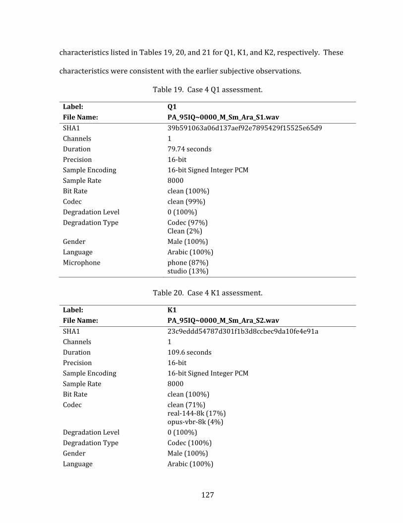
127
characteristics listed in Tables 19, 20, and 21 for Q1, K1, and K2, respectively. These
characteristics were consistent with the earlier subjective observations.
Table 19. Case 4 Q1 assessment.
Label: Q1 File Name: PA_95IQ~0000_M_Sm_Ara_S1.wav SHA1 39b591063a06d137aef92e7895429f15525e65d9 Channels 1 Duration 79.74 seconds Precision 16-bit Sample Encoding 16-bit Signed Integer PCM Sample Rate 8000 Bit Rate clean (100%) Codec clean (99%) Degradation Level 0 (100%) Degradation Type Codec (97%)
Clean (2%) Gender Male (100%) Language Arabic (100%) Microphone phone (87%)
studio (13%)
Table 20. Case 4 K1 assessment.
Label: K1 File Name: PA_95IQ~0000_M_Sm_Ara_S2.wav SHA1 23c9eddd54787d301f1b3d8ccbec9da10fe4e91a Channels 1 Duration 109.6 seconds Precision 16-bit Sample Encoding 16-bit Signed Integer PCM Sample Rate 8000 Bit Rate clean (100%) Codec clean (71%)
real-144-8k (17%) opus-vbr-8k (4%)
Degradation Level 0 (100%) Degradation Type Codec (100%) Gender Male (100%) Language Arabic (100%)

128
Microphone studio (100%)
Table 21. Case 4 K2 assessment.
Label: K2 File Name: PA_183IQ~000_M_Sm_Ara_S2.wav SHA1 2b2cc7db5e65d752061af4bc2ef1f3e65366e180 Channels 1 Duration 127.5 seconds Precision 16-bit Sample Encoding 16-bit Signed Integer PCM Sample Rate 8000 Bit Rate clean (100%) Codec clean (100%) Degradation Level 0 (100%) Degradation Type Codec (100%) Gender Male (100%) Language Unknown (99%)
Arabic (1%) Microphone phone (100%)
The extrinsic mismatch conditions include minor codec effects in K1. No
significant intrinsic mismatch conditions were discerned. The automated tools
correctly detected the Arabic language for Q1 and K1, but struggled with K2. Slightly
higher codec effects were detected in Q1. Detected degradation levels were minimal.
The duration and quality of the samples were deemed appropriate for processing with
the available tools.
Forensic Questions:
• How likely are the observed measurements between Q1 and K1 if the
samples originated from the same source vs. the samples originating from
different sources?

129
• How likely are the observed measurements between Q1 and K2 if the
samples originated from the same source vs. the samples originating from
different sources?
Case 4 Analysis and Processing
No additional data preparation or enhancement was required, and the data in
the Condition Set 1 data set was judged appropriate as a relevant population. The Q1,
K1, and K2 samples were submitted to the four algorithms, with the resulting plots
shown in Figures 79 through 94.
The plots for the GMM-UBM algorithm in Figures 79 through 83 reveal a good
discriminative capability for this data set, with an EER of between 1% and 2%. The
distributions exhibit good Gaussian statistics, and the DET plots are linear except for
some deviation at the extremes. The scores for Q1 against both K1 and K2 fall in the
target range, with the K2 score being noticeably higher. The score ranking lists both K1
and K2 high in the list, along with another (unknown) sample in the relevant
population. The 1v2 and 2v1 tests show comparable results.
The SVM plots in Figures 84 through 88 showed lower discrimination
performance than the GMM-UBM system, with EERs of 3% and 2% for the 1v2 and 2v1
tests, respectively. For this algorithm, Q1 more favorably compares to K1 in the 1v2
test, but scores for both K1 and K2 fall in the inconclusive or different-speaker range in
the 2v1 test. The score ranking concurs with these results.
The i-Vector results in Figures 89 through 91 show better discrimination
performance with an EER of approximately 1%, with the DET plot losing resolution due
to the reduced number of errors (because of the Rule of 30 again). The scores fall in the

130
non-target range, but the 1v2 score ranking shows K1 with the highest similarity to Q1.
The 2v1 reverse test shows the same Q1-K1 score, but ranks the truth-marked
companion to K2 as the highest similarity to K1.
The DNN results in Figures 92 through 94 show the best discrimination of the
four algorithms with an EER of approximately 0.5%. As with the i-Vector system, the
DET plot loses resolution with this accuracy for this data set. Despite the increased
performance, the system still generates scores in the inconclusive range for these
samples, and produces similar score rankings to the i-Vector system.
Figure 79. Case 4 (1v2) score distribution with GMM-UBM algorithm (K1 left, K2 right).

131
Figure 80. Case 4 (1v2) DET plot with GMM-UBM algorithm.
Figure 81. Case 4 (2v1) score distribution with GMM-UBM algorithm (K1 left, K2 right).

132
Figure 82. Case 4 (2v1) DET plot with GMM-UBM algorithm.
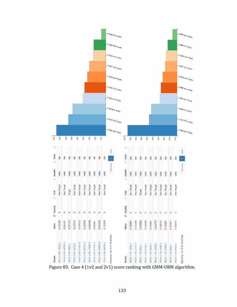
133
Figure 83. Case 4 (1v2 and 2v1) score ranking with GMM-UBM algorithm.
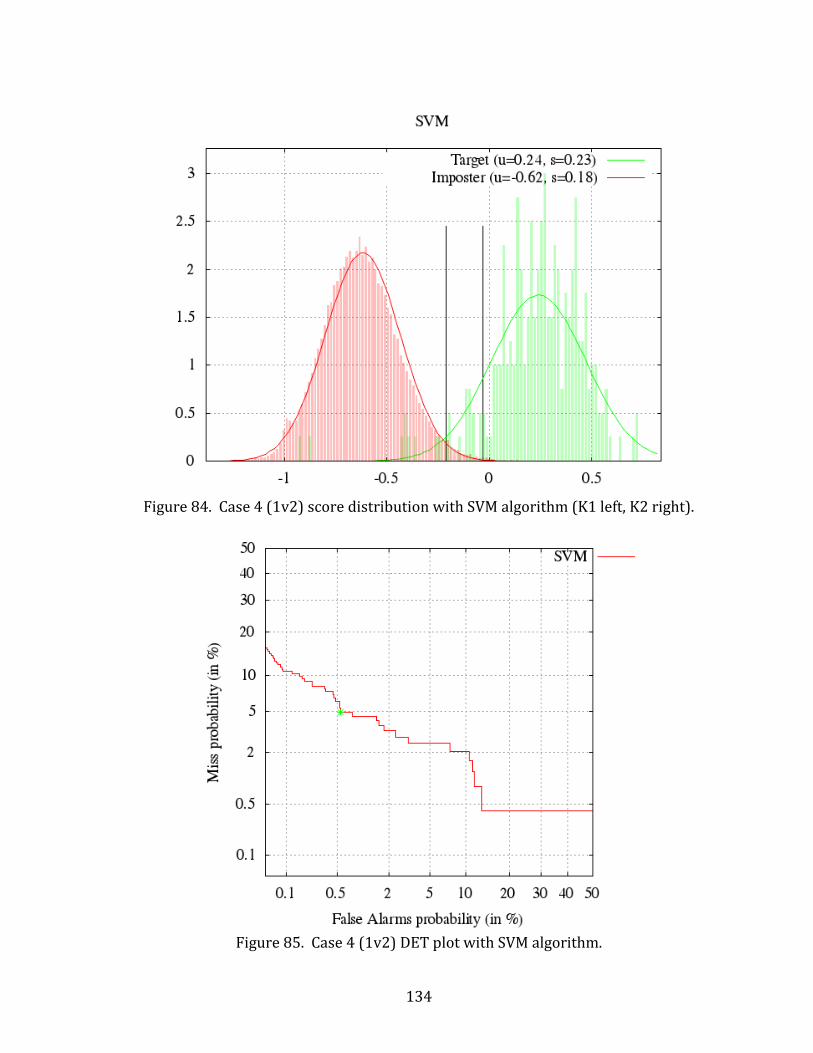
134
Figure 84. Case 4 (1v2) score distribution with SVM algorithm (K1 left, K2 right).
Figure 85. Case 4 (1v2) DET plot with SVM algorithm.

135
Figure 86. Case 4 (2v1) score distribution with SVM algorithm (K2 left, K1 right).
Figure 87. Case 4 (2v1) DET plot with SVM algorithm.

136
Figure 88. Case 4 (1v2 and 2v1) score ranking with SVM algorithm.
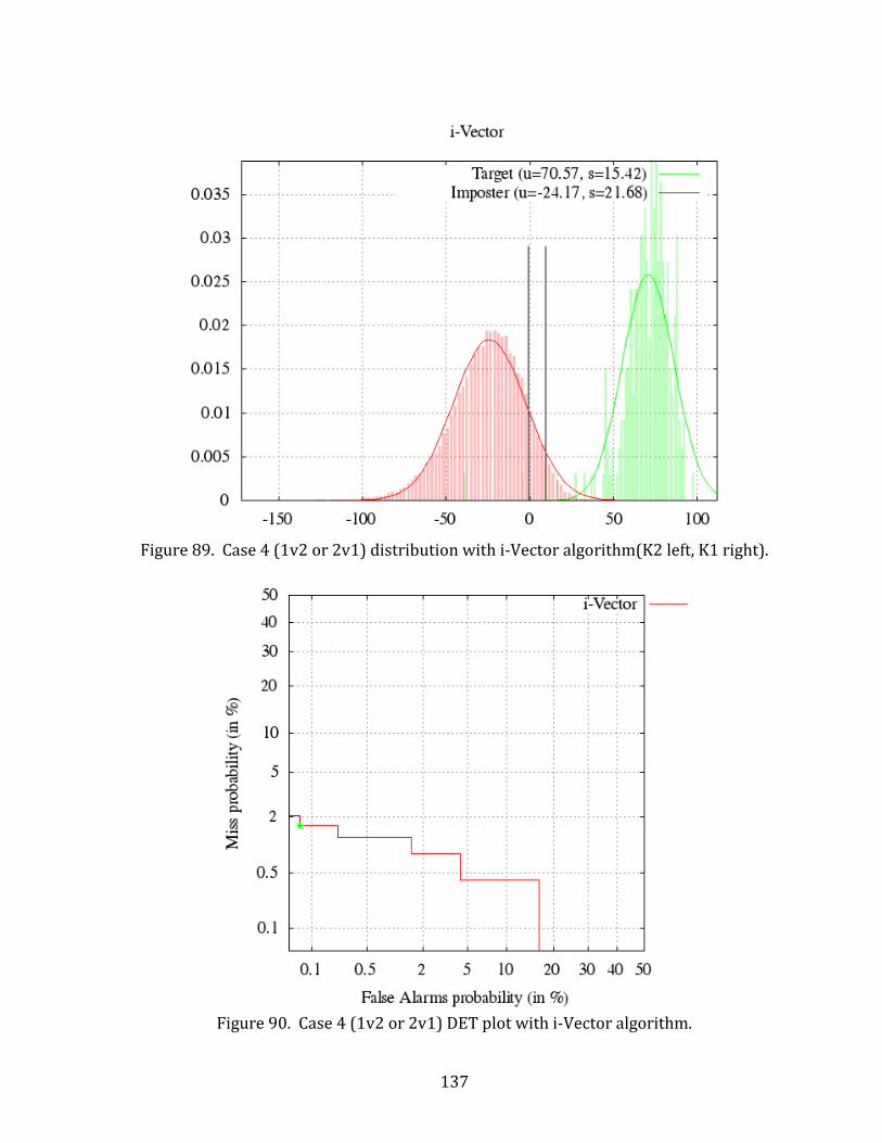
137
Figure 89. Case 4 (1v2 or 2v1) distribution with i-Vector algorithm(K2 left, K1 right).
Figure 90. Case 4 (1v2 or 2v1) DET plot with i-Vector algorithm.
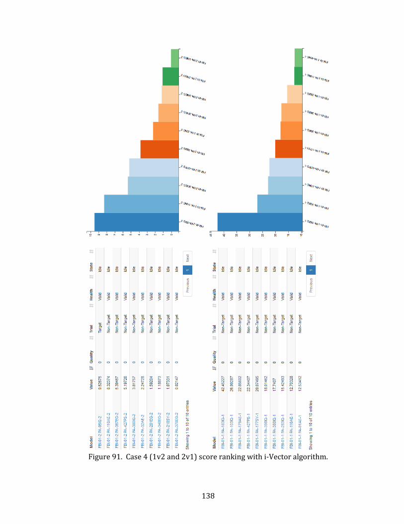
138
Figure 91. Case 4 (1v2 and 2v1) score ranking with i-Vector algorithm.

139
Figure 92. Case 4 (1v2 or 2v1) score distribution with DNN algorithm(K2 left, K1 right).
Figure 93. Case 4 (1v2 or 2v1) DET plot with DNN algorithm.
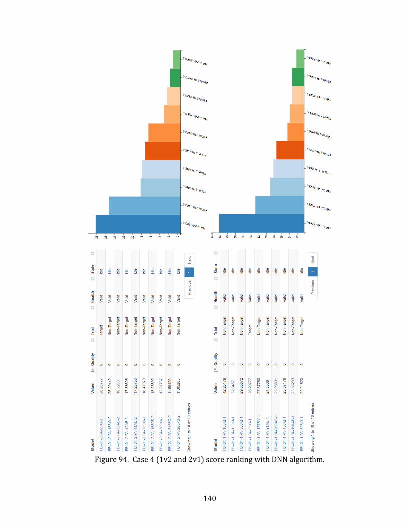
140
Figure 94. Case 4 (1v2 and 2v1) score ranking with DNN algorithm.

141
Table 22. Case 4 fusion results for Q1 vs. K1.
System Direction Score Collaboration Verbal GMM-UBM 1v2 0.2774 0.887 strong support for Hs GMM-UBM 2v1 0.2456 0.762 strong support for Hs SVM 1v2 -0.0326 0.975 strong support for Hs SVM 2v1 -0.2970 -0.430 weak support for Hd i-Vector n/a 9.5268 -0.996 strong support for Hd DNN n/a 28.2077 -0.944 strong support for Hd Fusion -0.211 inconclusive
Table 23. Case 4 fusion results for Q1 vs. K2.
System Direction Score Collaboration Verbal GMM-UBM 1v2 0.3325 0.990 strong support for Hs GMM-UBM 2v1 0.3068 0.981 strong support for Hs SVM 1v2 -0.2098 0.216 inconclusive SVM 2v1 -0.3699 -0.842 strong support for Hd i-Vector n/a -0.7212 -1.000 strong support for Hd DNN n/a 25.2944 -0.983 strong support for Hd Fusion -0.327 weak support for Hd
Case 4 Conclusions
Tables 22 and 23 show the corroboration measures and fusion results for the
Q1-K1 and Q1-K2 comparisons, respectively. The GMM-UBM system supports the
same-speaker hypothesis for both knowns, but the SVM shows inconsistent results. The
i-Vector and DNN systems yield corroboration measures that support the different-
speaker hypothesis for both knowns, but a visual check of the DNN score distribution
plot in Figure 92 shows that the scores are almost at the equal probability point (i.e.
inconclusive). The high discrimination of this system results in small values for P(E|Hs)
and P(E|Hd) in Equation (9), with the resulting division operation producing erratic
results.
142
The similar results in comparing Q1 to K1 and K2 are interesting, particularly
because the truth-marking indicates that K1 and K2 originate from different speakers.
The explanation could arise from one of four conditions:
• The Q1/K1 speaker is a lamb.
• The K2 speaker is a wolf.
• An undetected mismatch condition is affecting system operation. (This
condition is not likely, since all systems performed fairly consistently
between K1 and K2.)
• The truth-marking is incorrect.
The results for this case reinforce the lessons from Case Study 3 with respect to
understanding the configuration, reliability, and limitations of the tools in use. For
example, if the systems were trained with English data and evaluating Arabic vs. Arabic
samples (as opposed to English/English and English/non-English in the previous case
studies), the systems may be detecting similarities due to the common language instead
of to the speaker characteristics.
Answer to Forensic Question:
• Examination results are inconclusive for the Q1-K1 comparison.
• Examination results show weak support for the hypothesis that the Q1 and
K2 samples originate from different sources.
Case Study Summary
The case studies are four cases that, according to the truth-marking on the
samples, ideally would have resulted in high-similarity, unambiguous scores for the
same-speaker samples. While the algorithms used are firmly established as reliable

143
systems under well-characterized conditions (i.e. EERs typically under 5% and often as
low as 1%), the example cases show that an examiner must take care to use the tools in
conditions for which the tools have been validated. The cases also clearly show the
need for continued research toward improving the technology and for development of
processes for proper application of the technology.
144
CHAPTER IV
SUMMARY AND CONCLUSIONS
Although automated forensic speaker comparison is not a new idea, the
discipline is sufficiently challenging that few legal cases have involved the presentation
of the technology in open court. (The OSAC Legal Aspects of Speaker Recognition (LASR)
task group is currently developing an annotated listing of significant cases involving
speaker recognition[34].) In some cases (e.g. the Zimmerman trial [75]), expert
testimony on speaker recognition has been the subject of Daubert hearings to assess its
relevance and reliability, but ultimately the testimony was not presented for various
reasons. Some cases have been settled out of court and the records sealed, so no legal
precedent was established and the expert testimony was never revealed publicly. In
some cases, expert testimony has been used primarily to prevent the admission of
results from inappropriate use of the technology by the opposing counsel [76].
Despite limited exposure in the courtroom, the technology is used often in
investigatory settings where judicial requirements are not mandated. In this
environment, the technology has proven to be valuable, but the results from its use
sometimes are accepted with a degree of skepticism due to unverified performance in
problematic mismatch conditions.
The framework outlined in this paper aims to stimulate community discussion
for practical application of the noteworthy research achievements in forensic speaker
comparison using human-supervised automated methods. Much of the framework
relies on established procedures for handling and processing audio evidence, but

145
practices specific to FSC are much less standardized across the community (though
efforts are underway via the OSAC organization).
The NAS and PCAST reports present recommendations toward improving the
scientific basis of forensic science. Continued research efforts strive to support this
goal, but a significant fraction focuses on performance for the SRE. In a 2009 article,
Campbell [77] discussed the need for caution in forensic speaker recognition, and
commented on the direction of the speaker recognition community:
The evolution of speaker recognition, with a focus on error-rate reduction, progressively concentrates the research community on the engineering area, with less interest in the theoretical and analytical areas, involving phoneticians, for example. Nevertheless, it seems reasonable to develop automatic systems to aid in gaining a deeper understanding of the underlying phenomena.
At the time, the prevailing technology consisted of Gaussian Mixture Model
(GMM) systems in various combinations with Support Vector Machines (GMM-SVM)
and Factor Analysis (GMM-FA). In 2017, the technology has progressed to i-Vector
systems and Deep Neural Networks, and algorithm performance in concert with
advances in system calibration techniques continue to drive error rates lower, even as
test conditions become more diverse. With the prevalence of machine learning
techniques in current research trends, the pursuit of further improvements error rates
and better adaptation to mismatch conditions seems likely to continue.
However, research efforts must remain mindful of the entire process and not fall
victim to a single-minded drive to minimize error rates. The powerful machine learning
techniques available make it a relatively straightforward proposition to feed large
quantities of data into a system and evaluate the results, without necessarily
understanding the characteristics being learned by the system.

146
At the practitioner level, the availability of automated tools has simplified the
mechanics of conducting a forensic speaker comparison, and the tools will just as
readily provide results with appropriate or inappropriate data. Use of the technology
beyond its validated capabilities or configurations is not only a technical issue but also
an ethical one. Examiner judgement is still critical at multiple points in the process for
proper operation of those tools, and this judgement should be based on a sound
foundation of adoption of best practices; training of examiners; validation and
performance testing of tools, procedures, and examiners; and the adoption of and
adherence to ethical standards.
To address the NAS and PCAST recommendations, a good starting point would
be to focus on steps in the FSC process involving examiner judgement (as opposed to
steps based on automated processes that are more easily validated and less susceptible
to bias). Validation of human performance is difficult, time-consuming, expensive, and
prone to error, and the development of tools to assist in these judgement-based steps
would improve the overall process.
Challenges in the Relevant Population
The relevant population for a case often is selected by intuition based on
examiner judgement, and involves the selection of samples from existing sample sets or
(less frequently) obtaining additional samples. Samples can be selected by mismatch
conditions (see Table 2) such as language, microphone, transmission channel, gender,
etc., but with no standardized metrics support their suitability as members of the
relevant population. Tools to assist in the selection, or at the very least to calculate
metrics an examiner can use to assess the selection, could reduce the process variability

147
due to differences in examiner experience. Such an automated tool was used in the case
studies to assess various qualities of the samples (e.g. gender, codec, degradation, etc.),
but the tool is a research-quality tool and is not at all standardized.
Fusion for Multiple Algorithms
Calibration is an active area of research in the speaker recognition community
[61], but current methods require a significant quantity of data (the Rule of 30 again).
Practitioners frequently do not have enough data to perform such a calibration and
must rely on alternative approaches that are less precise. This situation is exacerbated
by the need to select a relevant population, which further reduces the available data as
per the paradox mentioned in Case Study 1. The proposed framework addresses this
issue by the development of an objectively-measured consensus of multiple systems
using a corroboration algorithm, but this method has not been researched extensively.
More research in this area is still needed.
Verbal Scale Standards for Reporting Results
The need to convert scientific conclusions to the non-scientific community is an
ongoing challenge, though attempts continue toward improving communication [78]
[79]. An OSAC draft document, Standards for expressing source conclusions [80],
attempts to address the issue of presenting verbal examination results, but the
document is highly controversial and is still under debate. More research is still
needed.
148
Data and Standards for Validation
The paradigm shift of empirically grounded science discussed by Saks [28] and
currently driven by the significant investment in the OSAC establishment encourages
the community to objectively assess algorithm and system performance. However, the
available data sets for such assessment typically contain research data and are less
representative of real-world conditions. The few corpora that do represent such
conditions are only available with limited access (e.g. law enforcement, government
agencies, etc.). The speaker recognition community is in need of a standardized
validation process that includes a representative data set of real-world conditions.
149
REFERENCES
[1] National Research Council, Strengthening Forensic Science in the United States: A Path Forward. 2009.
[2] “Forensic Science in Criminal Courts: Ensuring Scientific Validity of Feature-Comparison Methods.” President’s Council of Advisors on Science and Technology, Sep-2016.
[3] J. P. Campbell, “Speaker recognition: A tutorial,” Proc. IEEE, vol. 85, no. 9, pp. 1437–1462, 1997.
[4] P. Rose, Forensic Speaker Identification. London ; New York: Taylor & Francis, 2002.
[5] D. Hallimore and M. Piper, “SWGDE Best Practices for Forensic Audio,” in Audio Engineering Society Conference: 33rd International Conference: Audio Forensics-Theory and Practice, 2008.
[6] “SWGDE Best Practices for Digital Audio Authentication.” SWGDE, 08-Oct-2016.
[7] B. E. Koenig and D. S. Lacey, “Forensic authentication of digital audio recordings,” J. Audio Eng. Soc., vol. 57, no. 9, pp. 662–695, 2009.
[8] “A Quick Summary of The National Academy of Sciences Report | The Truth About Forensic Science.” [Online]. Available: http://www.thetruthaboutforensicscience.com/a-quick-summary-of-the-national-academy-of-sciences-report-on-forensic-sciene/. [Accessed: 29-Jan-2017].
[9] “Occam’s razor - definition of Occam’s razor by The Free Dictionary.” [Online]. Available: http://www.thefreedictionary.com/Occam%27s+razor. [Accessed: 29-Jan-2017].
[10] H. Andersen and B. Hepburn, “Scientific Method,” in The Stanford Encyclopedia of Philosophy, Summer 2016., E. N. Zalta, Ed. Metaphysics Research Lab, Stanford University, 2016.
[11] “List of cognitive biases,” Wikipedia. 13-Jan-2017.
[12] T. G. Gutheil and R. I. Simon, “Avoiding bias in expert testimony,” Psychiatr. Ann., vol. 34, no. 4, pp. 260–270, 2004.
[13] K. Cherry, “What Is a Cognitive Bias? Definition and Examples,” Verywell, 09-May-2016. [Online]. Available: https://www.verywell.com/what-is-a-cognitive-bias-2794963. [Accessed: 03-Feb-2017].

150
[14] S. M. Kassin, I. E. Dror, and J. Kukucka, “The forensic confirmation bias: Problems, perspectives, and proposed solutions,” J. Appl. Res. Mem. Cogn., vol. 2, no. 1, pp. 42–52, 2013.
[15] I. E. Dror, “HOW CAN FRANCIS BACON HELP FORENSIC SCIENCE? THE FOUR IDOLS OF HUMAN BIASES,” Jurimetrics, vol. 50, no. 1, pp. 93–110, 2009.
[16] T. Simoncelli, “Rigor in Forensic Science,” in Blinding as a Solution to Bias, San Diego: Academic Press, 2017, pp. 129–131.
[17] U. S. D. of J. O. of the I. General, A Review of the FBI’s Handling of the Brandon Mayfield Case. US Department of Justice, Office of the Inspector General, Oversight and Review Division, 2006.
[18] I. E. Dror and D. Charlton, “Why Experts Make Errors - ProQuest,” J. Forensic Identif., vol. 56, no. 4, pp. 600–616, Feb. 2006.
[19] T. Sharot, “The optimism bias,” Curr. Biol., vol. 21, no. 23, pp. R941–R945, Dec. 2011.
[20] N. Venville, “A Review of Contextual Bias in Forensic Science and its potential Legal Implications.” Australia New Zealand Policing Advisory Agency, Dec-2010.
[21] G. Edmond, J. M. Tangen, R. A. Searston, and I. E. Dror, “Contextual bias and cross-contamination in the forensic sciences: the corrosive implications for investigations, plea bargains, trials and appeals,” Law Probab. Risk, vol. 14, no. 1, pp. 1–25, Mar. 2015.
[22] M. J. Saks and J. J. Koehler, “The Individualization Fallacy in Forensic Science Evidence,” Social Science Research Network, Rochester, NY, SSRN Scholarly Paper ID 1432516, 2008.
[23] N. J. Schweitzer and M. J. Saks, “The CSI effect: popular fiction about forensic science affects the public’s expectations about real forensic science,” Jurimetrics, pp. 357–364, 2007.
[24] W. C. Thompson and E. L. Schumann, “Interpretation of statistical evidence in criminal trials: The prosecutor’s fallacy and the defense attorney’s fallacy.,” Law Hum. Behav., vol. 11, no. 3, p. 167, 1987.
[25] W. C. Thompson, “Painting the target around the matching profile: the Texas sharpshooter fallacy in forensic DNA interpretation,” Law Prob Risk, vol. 8, p. 257, 2009.
[26] K. Inman and N. Rudin, “Sequential Unmasking: Minimizing Observer Effects in Forensic Science,” in Encyclopedia of Forensic Sciences, Second., 2013, pp. 542–548.

151
[27] I. E. Dror, D. Charlton, and A. E. Péron, “Contextual information renders experts vulnerable to making erroneous identifications,” Forensic Sci. Int., vol. 156, no. 1, pp. 74–78, 2006.
[28] M. J. Saks and J. J. Koehler, “The coming paradigm shift in forensic identification science,” Science, vol. 309, no. 5736, pp. 892–895, 2005.
[29] C. G. G. Aitken, F. Taroni, and A. Biedermann, “Statistical Interpretation of Evidence: Bayesian Analysis,” in Encyclopedia of Forensic Sciences, Second., 2013, pp. 292–297.
[30] G. S. Morrison, “Forensic voice comparison and the paradigm shift,” Sci. Justice, vol. 49, no. 4, pp. 298–308, Dec. 2009.
[31] G. Villejoubert and D. R. Mandel, “The inverse fallacy: An account of deviations from Bayes’s theorem and the additivity principle,” Mem. Cognit., vol. 30, no. 2, pp. 171–178, Mar. 2002.
[32] “Federal Rules of Evidence.” U. S. Government Printing Office, 01-Dec-2014.
[33] US v. Vallejo, vol. 237. 2001, p. 1008.
[34] D. Glancy, “SR Subcommittee Joint Discussion with LRC and HFC - April 19, 2017, Materials Regarding Court Decisions Regarding ‘Earwitness’ Testimony,” 14-Apr-2017.
[35] Frye v. United State, vol. 293. 1923, p. 1013.
[36] A. Blank, M. Maddox, and B. Goodrich, “Analysis of Frye and its progeny,” 26-Jul-2013.
[37] Daubert v. Merrell Dow Pharmaceuticals, Inc., vol. 509. 1993, p. 579.
[38] A. Blank and M. Maddox, “Analysis of Daubert and its progeny,” 13-Mar-2013.
[39] General Electric Co. v. Joiner, vol. 522. 1997, p. 136.
[40] United States v. McKeever, vol. 169. 1958, p. 426.
[41] “Daubert v. Frye - A State-by-State Comparison.” [Online]. Available: https://www.theexpertinstitute.com/daubert-v-frye-a-state-by-state-comparison/. [Accessed: 28-Jan-2017].
[42] “Daubert and Frye in the 50 States | JuriLytics.” [Online]. Available: https://jurilytics.com/50-state-overview. [Accessed: 28-Jan-2017].
152
[43] “Speaker Recognition Evaluation 2016 | NIST.” [Online]. Available: https://www.nist.gov/itl/iad/mig/speaker-recognition-evaluation-2016. [Accessed: 13-Feb-2017].
[44] G. Doddington, W. Liggett, A. Martin, M. Przybocki, and D. Reynolds, “Sheep, goats, lambs and wolves: A statistical analysis of speaker performance in the NIST 1998 speaker recognition evaluation,” DTIC Document, 1998.
[45] A. Martin, G. Doddington, T. Kamm, M. Ordowski, and M. Przybocki, “The DET Curve In Assessment Of Detection Task Performance,” DTIC Document, 1997.
[46] gnu_detware. National Institute of Standards and Technology.
[47] L. G. Kersta, “Voiceprint‐Identification Infallibility,” J. Acoust. Soc. Am., vol. 34, no. 12, pp. 1978–1978, Dec. 1962.
[48] R. Vanderslice and P. Ladefoged, “The ‘Voiceprint’ Mystique,” J. Acoust. Soc. Am., vol. 42, no. 5, pp. 1164–1164, Nov. 1967.
[49] US v. Bahena, vol. 223. 2000, p. 797.
[50] US v. Angleton, vol. 269. 2003, p. 892.
[51] “Zimmerman Case: Dr. Hirotaka Nakasone, FBI, and the low-quality 3-second audio file,” Le·gal In·sur·rec·tion, 07-Jun-2013. .
[52] J. Smith, “Introduction to Media Forensics,” presented at the MSRA 5124 - Forensic Science and Litigation, National Center for Media Forensics, 19-Aug-2013.
[53] J. L. Ramirez, “Effects of Clipping Distortion on an Automatic Speaker Recognition System.” University of Colorado, 28-Apr-2016.
[54] M. Graciarena, M. Delplanche, E. Shriberg, A. Stolcke, and L. Ferrer, “Acoustic front-end optimization for bird species recognition,” in Acoustics Speech and Signal Processing (ICASSP), 2010 IEEE International Conference on, 2010, pp. 293–296.
[55] M. Graciarena, M. Delplanche, E. Shriberg, and A. Stolcke, “Bird species recognition combining acoustic and sequence modeling,” in Acoustics, Speech and Signal Processing (ICASSP), 2011 IEEE International Conference on, 2011, pp. 341–344.
[56] “MediaInfo.” [Online]. Available: https://mediaarea.net/en/MediaInfo. [Accessed: 13-Apr-2017].
[57] “Tools | NIST.” [Online]. Available: https://www.nist.gov/itl/iad/mig/tools. [Accessed: 13-Apr-2017].

153
[58] R. Schwartz, J. P. Campbell, and W. Shen, “When to Punt on Speaker Comparison,” presented at the ASA Forensic Acoustics Subcommittee 2011, San Diego, California, 03-Nov-2011.
[59] A. Drygajlo, M. Jessen, S. Gfroerer, I. Wagner, J. Vermeulen, and T. Niemi, “Methodological Guidelines for Best Practice in Forensic Semiautomatic and Automatic Speaker Recognition.” European Network of Forensic Science Institutes, 2015.
[60] V. Hughes and P. Foulkes, “The relevant population in forensic voice comparison: Effects of varying delimitations of social class and age,” Speech Commun., vol. 66, pp. 218–230, Feb. 2015.
[61] N. Brummer, “Measuring, refining and calibrating speaker and language information extracted from speech.” University of Stellenbosch, 2010.
[62] N. Brummer, “The BOSARIS Toolkit: Theory, Algorithms and Code for Surviving the New DCF.” Dec-2011.
[63] G. R. Doddington, “Speaker recognition evaluation methodology: a review and perspective,” in Proceedings of RLA2C Workshop: Speaker Recognition and its Commercial and Forensic Applications, Avignon, France, 1998, pp. 60–66.
[64] J. Sprenger, “From Evidential Support to a Measure of Corroboration,” 2014.
[65] G. E. Box, “Robustness in the strategy of scientific model building,” Robustness Stat., vol. 1, pp. 201–236, 1979.
[66] L. H. Tribe, “Trial by mathematics: Precision and ritual in the legal process,” Harv. Law Rev., pp. 1329–1393, 1971.
[67] M. O. Finkelstein and W. B. Fairley, “The Continuing Debate Over Mathematics in the Law of Evidence: A Comment on‘ Trial by Mathematics,’” Harv. Law Rev., pp. 1801–1809, 1971.
[68] P. Tillers, “Trial by mathematics—reconsidered,” Law Probab. Risk, vol. 10, no. 3, pp. 167–173, 2011.
[69] “ENFSI Guideline for Evaluative Reporting in Forensic Science (Version 3.0).” European Network of Forensic Science Institutes.
[70] A. Nordgaard, R. Ansell, W. Drotz, and L. Jaeger, “Scale of conclusions for the value of evidence,” Law Probab. Risk, vol. 11, no. 1, pp. 1–24, Mar. 2012.
[71] D. A. Reynolds, “Speaker identification and verification using Gaussian mixture speaker models,” Speech Commun., vol. 17, no. 1, pp. 91–108, 1995.

154
[72] W. M. Campbell, J. P. Campbell, D. A. Reynolds, E. Singer, and P. A. Torres-Carrasquillo, “Support vector machines for speaker and language recognition,” Comput. Speech Lang., vol. 20, no. 2, pp. 210–229, 2006.
[73] P. Kenny, P. Ouellet, N. Dehak, V. Gupta, and P. Dumouchel, “A study of interspeaker variability in speaker verification,” IEEE Trans. Audio Speech Lang. Process., vol. 16, no. 5, pp. 980–988, 2008.
[74] F. Richardson, D. Reynolds, and N. Dehak, “A unified deep neural network for speaker and language recognition,” ArXiv Prepr. ArXiv150400923, 2015.
[75] “George Zimmerman Trial,” Le·gal In·sur·rec·tion. .
[76] “Zimmerman Prosecution’s Voice Expert admits: ‘This is not really good evidence,’” Le·gal In·sur·rec·tion, 08-Jun-2013. .
[77] J. P. Campbell, W. Shen, W. M. Campbell, R. Schwartz, J.-F. Bonastre, and D. Matrouf, “Forensic speaker recognition,” IEEE Signal Process. Mag., vol. 26, no. 2, 2009.
[78] G. Jackson, “Understanding forensic science opinions,” in Handbook of Forensic Science, 1st ed., J. Frasier and R. Williams, Eds. Cullompton, Devon, UK: Willan, 2009, pp. 419–445.
[79] G. Jackson, D. Kaye, C. Neumann, A. Ranadive, and V. Reyna, “Communicating the Results of Forensic Science Examinations.” 08-Nov-2015.
[80] “Standard for expressing source conclusions.” OSAC - Pattern and Digital SAC, 01-Feb-2016.

155
INDEX
accent ...................................... 40, 88, 90, 103 aural-perceptual method ......................... 42 authentication .............................................. 22 Bayes Factor .................................................. 18 Bayes’ Rule .................................................... 18 Bayes’ Theorem ........................................... 18 best evidence ......................................... 19, 47 best practices ................................................... 5 bias.................................................................. 8, 9
base rate fallacy ................................ 12, 28 cognitive .................................. 9, 15, 40, 42 confirmation ...................................... 10, 16 contextual .................................................. 11 defender’s fallacy .................................... 14 expectation effect ................................... 10 framing effect ........................................... 12 individualization fallacy ....................... 13 mitigation .................................................. 14 motivational.............................................. 10 optimism .................................................... 11 prosecutor’s fallacy ................................ 13 sharpshooter’s fallacy ........................... 14 statistical ............................................. 12, 16 uniqueness fallacy .................................. 13
bird call .................................................... 51, 56 BOSARIS toolkit ........................................... 60 calibration ...................................................... 59 case manager ................................................ 45 chain of evidence ......................................... 43 clipping ............................................ 26, 51, 52 conclusion iv, 2, 3, 4, 8, 12, 15, 24, 40, 64,
67, 87, 102, 124, 141, 147 corpus
Bilingual .................................................. 102 CrossInt ................................................... 102 NIST’99 ....................................................... 70 NoTel ........................................................... 87 PanArabic ............................................... 125
critical listening ........................................... 42 CSI effect ......................................................... 13 Daubert .................................. 23, 24, 25, 144
criteria ......................................... 23, 25, 43 decision maker ........................................ 7, 19
DET plot... xviii, 32, 34, 36, 37, 73, 74, 91, 106, 107, 129, 130
detection task ............................................... 17 DNN ...................... 69, 74, 91, 107, 130, 145 earwitness ..................................................... 22 EER ......................................................... xviii, 31 ENFSI ...................................... xviii, 55, 61, 65 extrinsic .. 26, 51, 52, 53, 72, 90, 105, 128 factor analysis ............................................ 145 FBI .................................................. xviii, 42, 68
FAVIAU ...................................... vii, xviii, 68 Federal Rules of Evidence ....................... 19
Rule 401 ..................................................... 20 Rule 402 ..................................................... 20 Rule 403 ..................................................... 20 Rule 702 ........................ 21, 23, 24, 42, 64 Rule 705 ..................................................... 21 Rule 901 ....................................... 22, 24, 42
filtering ........................................................... 57 forensic question .................. 44, 48, 64, 67 framing the question .......................... 15, 16 Frye ..................................................... 23, 24, 25 fundamental principle .............................. 47 GE v. Joiner .................................................... 23 GMM-UBM ... xviii, 69, 73, 74, 90, 91, 106,
129 goat ................................................................... 30 intrinsic ......... 26, 51, 52, 72, 90, 105, 128 ipse dixit ......................................................... 24 i-Vector 59, 66, 69, 74, 91, 107, 129, 130,
145 lamb ....................................................... 30, 142 language
Arabic ... 40, 53, 68, 125, 126, 127, 128, 142
Bengali ...................................................... 102 English .... 54, 56, 60, 68, 70, 71, 72, 87,
88, 90, 102, 103, 104, 105, 126, 142 Hindi .......................................................... 102 Kannada ................................................... 102 Korean .............................................. 68, 102 Malayalam ............................................... 102 Marathi ..................................................... 102 Punjabi ..................................................... 102
156
Spanish .............................. 56, 60, 68, 102 Tamil ........................... 102, 103, 104, 107 Urdu ............................................................. 53
likelihood ratio 17, 18, 28, 30, 39, 49, 66, 69
machine learning......................................... 27 McKeever ....................................................... 24 MediaInfo ....................................................... 52 message digest ............................................. 50 mismatch .... 26, 29, 40, 51, 52, 53, 60, 72,
90, 91, 105, 128, 144, 145, 146 NAS ........................................................... xviii, 1 National Academy of Sciences 1, 3, 7, 14,
145, 146 National Research Council.......................... 1 NIST .................................. vii, xviii, 29, 32, 52 noise ................................................................. 57 Occam’s Razor ................................................. 7 OSAC ................................... vii, xviii, 145, 148
Digital Evidence ......................................... 6 Speaker Recognition ............ vii, xviii, 41
paradigm shift .................................... 16, 148 paradox .......................................... 58, 74, 147 partitioning .................................... 39, 40, 59 PCAST .................................. xviii, 1, 145, 146 PLDA ................................................................ 59 probability inversion ................................. 18 punt .................................................................. 54 purification .................................................... 56 relevant population ...... 24, 37, 39, 40, 48,
49, 53, 55, 58, 68
Rule of 30 ............................ 61, 73, 129, 147 scientific method ............................ 8, 21, 23 Scientific Working Group ..................... xviii sequential unmasking ........................ 15, 46 sheep ............................................................... 30 similarity .. 17, 28, 29, 49, 69, 73, 91, 106,
107, 130, 142 SNR ......................................................... xviii, 52 SPQA ...................................................... xviii, 52 SRE .......................................... xviii, 29, 32, 90 strength of evidence ............... 7, 17, 39, 49 SVM ........... xviii, 69, 74, 91, 106, 129, 145 SWG
Digital Evidence .............................. xviii, 6 trial by mathematics.................................. 64 trier of fact . iv, 2, 7, 17, 18, 20, 21, 22, 59,
64, 67 typicality .......................................... 17, 40, 59 universal background model (UBM) ... 28 V&V .................................................................. 43 validation ....................................................... 51 variation
between-speaker ....................................... 5 channel .......................................................... 5 inter-speaker .............................................. 5 intra-speaker .............................................. 5 within-speaker ........................................... 5
weight of evidence ....................... 18, 48, 50 wolf ........................................................ 30, 142 Zimmerman ........................................ 42, 144