A Framework for Real-TimeHigh-Throughput Signal and ImageProcessing Systems on Workstations

Prof. Brian L. Evansin collaboration with

Gregory E. Allen and K. Clint Slatton

Department of Electrical and Computer EngineeringThe University of Texas at Austin

http://www.ece.utexas.edu/~bevans/

Outline

• Introduction and Motivation

• Background

• Framework and Implementation

• Case Study #1: 3-D Sonar Beamformer

• Case Study #2: SAR Processor

• Conclusion

2

Introduction• High-performance, low-volume applications

(~100 MB/s I/O; 1-20 GFLOPS; under 50 units)

3

• Sonar beamforming

• Synthetic aperture radar (SAR) image processing

• Multichannel image restoration at video rates

• Current real-time implementation technologies

• Custom hardware

• Custom integration using commercial-off-the-shelf (COTS) processors (e.g. 100 digital signal processors in a VME chassis)

• COTS software development is problematic

• Development and debugging tools are generally immature

• Partitioning is highly dependent on hardware topology

Workstation Implementations• Multiprocessor workstations are commodity items

• Up to 64 processors for Sun Enterprise servers

• Up to 14 processors for Compaq AlphaServer ES

• Symmetric multiprocessing (SMP) operating systems

• Dynamically load balances many tasks on multiple processors

• Lightweight threads (e.g. POSIX Pthreads)

• Fixed-priority real-time scheduling

• Leverage native signal processing (NSP) kernels

• Software development is faster and easier

4

• Development environment and target architecture are same

• Development can be performed on less powerful workstations

Parallel Programming• Problem: Parallel programming is difficult

• Hard to predict deadlock

• Non-determinate execution

• Difficult to make scalable software (e.g. rendezvous models)

• Solution: Formal models for programming

• We develop a model that leverages SMP hardware

5

• Utilizes the formal bounded Process Network model

• Extends with firing thresholds from Computation Graphs

• Models overlapping algorithms on continuous streams of data

• We provide a high-performance implementation

Motivation

4-GFLOP sonar beamformers; volumes of under 50 units; 1999 technology

6

CustomHardware

EmbeddedCOTS

CommodityWorkstation

Development cost

Development time

Physical size (m3)

Reconfigurability

Software portability

Hardware upgradability

$2000K $500K $100K

24 months 12 months 6 months

3.0 3.0 4.0

low medium high

low medium high

low medium high

Outline

• Introduction and Motivation

• Background

• Framework and Implementation

• Case Study #1: 3-D Sonar Beamformer

• Case Study #2: SAR Processor

• Conclusion

7

Native Signal Processing• Single-cycle multiply-accumulate (MAC) operation

• Vector dot products, digital filters, and correlation

• Missing extended precision accumulation

• Single-instruction multiple-data (SIMD) processing

• UltraSPARC Visual Instruction Set (VIS) and Pentium MMX: 64-bit registers, 8-bit and 16-bit fixed-point arithmetic

• Pentium III, K6-2 3DNow!: 64-bit registers, 32-bit floating-point

• PowerPC AltiVec: 128-bit registers, 4x32 bit floating-point MACs

• Saturation arithmetic (Pentium MMX)

• Software data prefetching to prevent pipeline stalls

• Must hand-code using intrinsics and assembly code8

iα ixi=1

N∑

Dataflow Models

• Each node represents a computational unit

• Each edge represents a one-way FIFO queue of data

• Models parallelism

• A program is represented as a directed graph

PBA

• A node may have any number of input or output edges, and may communicate only via these edges

CGSDF

Synchronous Dataflow (SDF)Computation Graphs (CG)Boolean Dataflow (BDF)Dynamic Dataflow (DDF)Process Networks (PN)

more general9

BDF DDF PN

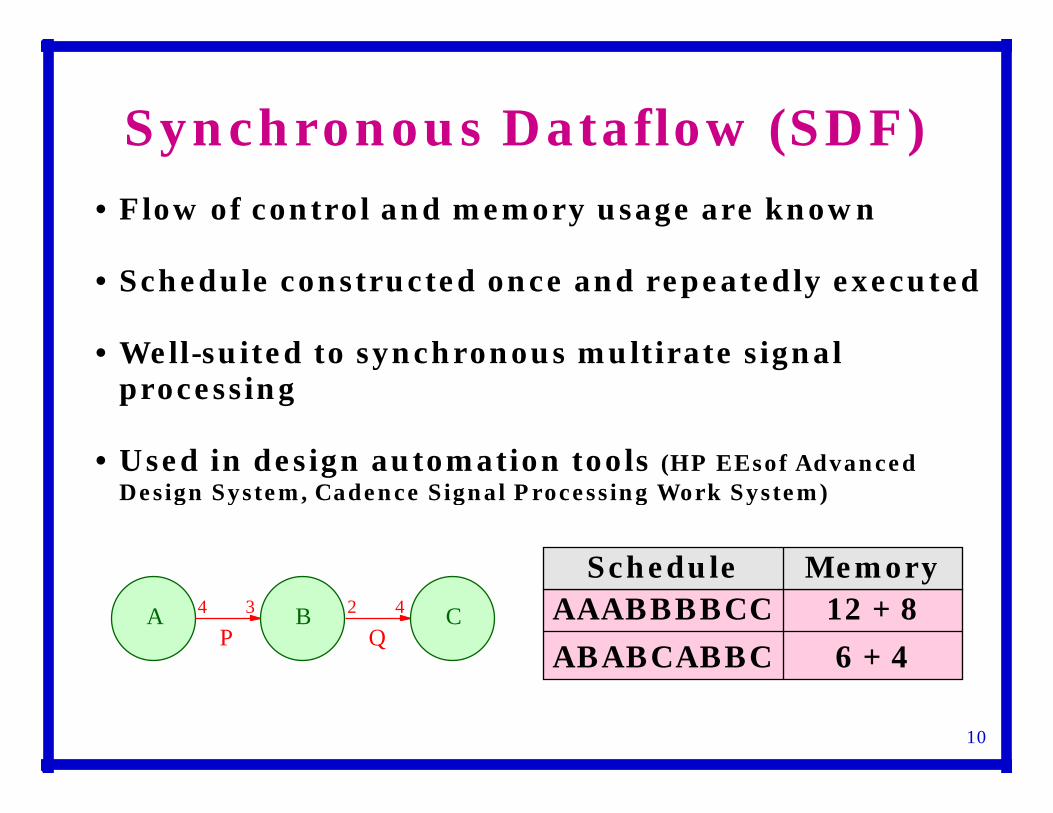
• Flow of control and memory usage are known

• Schedule constructed once and repeatedly executed

• Well-suited to synchronous multirate signal processing

• Used in design automation tools (HP EEsof Advanced Design System, Cadence Signal Processing Work System)

Synchronous Dataflow (SDF)

10

AP

BQ

C4 3 2 4

Schedule MemoryAAABBBBCC

ABABCABBC

12 + 8

6 + 4

Computation Graphs (CG)

• Each FIFO queue is parametrized [Karp & Miller, 1966]

A is number of data words initially present

U is number of words inserted by producer on each firing

W is number of words removed by consumer on each firing

T is number of words in queue before consumer can fire

where T ≥ W

11

• Termination and boundedness are decidable

• Computation graphs are statically scheduled

• Iterative static scheduling algorithms

• Synchronous Dataflow is T = W for every queue

• A networked set of Turing machines

• Concurrent model (superset of dataflow models)

• Mathematically provable properties [Kahn, 1974]

Process Networks (PN)

12

• Suspend execution when trying to consume data from an empty queue (blocking reads)

• Never suspended for producing data (non-blocking writes) so queues can grow without bound

• Dynamic firing rules at each node

• Guarantees correctness

• Guarantees determinate execution of programs

• Enables easier development and debugging

Bounded Scheduling

• Infinitely large queues cannot be realized

• Dynamic scheduling to always execute the program in bounded memory if it is possible [Parks, 1995]:

1. Block when attempting to read from an empty queue

2. Block when attempting to write to a full queue

3. On artificial deadlock, increase the capacity of the smallest full queue until its producer can fire

• Preserves formal properties: liveness, correctness, and determinate execution

• Maps well to a threaded implementation(one node maps to one thread)

13

Outline

• Introduction and Motivation

• Background

• Framework and Implementation

• Case Study #1: 3-D Sonar Beamformer

• Case Study #2: SAR Processor

• Conclusion

14

Framework

• Utilize the Process Network model [Kahn, 1974]

• Utilize bounded scheduling [Parks, 1995]

• Models overlapping algorithms on continuous streams of data(e.g. digital filters)

• Decouples computation (node) from communication (queue)

• Allows compositional parallel programming

15

• Captures concurrency and parallelism

• Provides correctness and determinate execution

• Permits realization in finite memory

• Preserves properties regardless of which scheduler is used

• Extend this model with firing thresholds

• Low-overhead, high-performance, and scalable

• Publicly available source code

Implementation

• Designed for real-time high-throughput signal processing systems based on proposed framework

• Implemented in C++ with template data types

• POSIX Pthread class library

• Portable to many different operating systems

• Optional fixed-priority real-time scheduling

http://www.ece.utexas.edu/~allen/PNSourceCode/16

• Node granularity larger than thread context switch

Implementation: Nodes

Pthread Pthread

• Each node corresponds to a Pthread

17

• Context switch is about 10 µs in Sun Solaris operating system

• Increasing node granularity reduces overhead

• Thread scheduler dynamically schedules nodes as the flow of data permits

• Efficient utilization of multiple processors (SMP)

• Compensates for lack of hardware support for circular buffers (e.g. modulo addressing in DSPs)

• Queues tradeoff memory usage for overhead

• Virtual memory manager keeps data circularity in hardware

Implementation: Queues

Mirror regionQueue data region

Mirrored data

• Nodes operate directly on queue memory to avoid unnecessary copying

• Queues use mirroring to keep data contiguous

18

A Sample Node

• A queue transaction uses pointers

inputQNode

outputQ

typedef float T;while (true) {

// blocking calls to get in/out data pointers const T* inPtr = inputQ.GetDequeuePtr(inThresh); T* outPtr = outputQ.GetEnqueuePtr(outThresh);

DoComputation( inPtr, inThresh, outPtr, outSize );

// complete node transactions inputQ.Dequeue(inSize); outputQ.Enqueue(outSize);}

19

• Decouples communication and computation

• Overlapping streams without copying

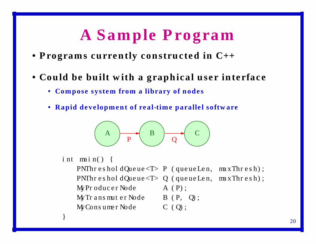
int main() {PNThresholdQueue<T> P (queueLen, maxThresh);PNThresholdQueue<T> Q (queueLen, maxThresh);MyProducerNode A (P);MyTransmuterNode B (P, Q);MyConsumerNode C (Q);

}

A Sample Program

AP

BQ

C

• Programs currently constructed in C++

• Could be built with a graphical user interface

20

• Compose system from a library of nodes

• Rapid development of real-time parallel software

Case Study #1: Sonar Beamformer

21

• Collaboration with UT Applied Research Laboratories

HazardBeamcoverage

Side view(vertical coverage)

Top view(horizontal coverage)

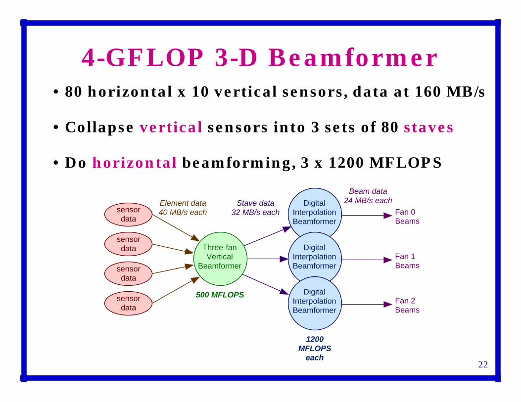
4-GFLOP 3-D Beamformer

sensordata

sensordata

sensordata

sensordata

Element data40 MB/s each

Three-fanVertical

Beamformer

Stave data32 MB/s each

DigitalInterpolationBeamformer

DigitalInterpolationBeamformer

DigitalInterpolationBeamformer

500 MFLOPS

1200MFLOPS

each

Fan 0Beams

Fan 1Beams

Fan 2Beams

• 80 horizontal x 10 vertical sensors, data at 160 MB/s

• Collapse vertical sensors into 3 sets of 80 staves

• Do horizontal beamforming, 3 x 1200 MFLOPS

22

Beam data24 MB/s each

Multiple vertical transducers for every horizontal position

stave

Vertical Beamformer

• Vertical columns combined into 3 stave outputs

• Multiple integer dot products

• Convert integer to floating-point for following stages

• Interleave output data for following stages

• Kernel implementation on UltraSPARC-II

• VIS for fast dot products and floating-point conversion

• Software data prefetching to hide memory latency

• Operates at 313 MOPS at 336 MHz (93% of peak)23

• Different beams formed from same data

• Kernel implementation on UltraSPARC-II

Horizontal Beamformer

Interpolate z-N1

Interpolate z-NM

Σ b[n]••

••

Digital Interpolation Beamformer

Stave data atinterval ∆

Interpolate up tointerval δ = ∆/L

Time delayat interval δα1

αM

• Sample at just above the Nyquist rate, interpolate to obtain desired time delay resolution

• Highly optimized C++ (loop unrolling and SPARCompiler5.0DR)

• Operates at 440 MFLOPS at 336 MHz (60% of peak)24

Singlebeam output

Performance Results• Sun Ultra Enterprise 4000 with twelve 336-MHz

UltraSPARC-IIs, 3 Gb RAM, running Solaris 2.6

• Compare to sequential case and thread pools

0 2 4 6 8 10 120

500

1000

1500

2000

2500

3000

3500

4000

4500

5000

CPUs

Performance vs. Number of processors

• Speedup is 11.28 and efficiency of 94%

• Runs real-time +14%25

• On one CPU, slowdown < 0.5%

• 8 CPUs vs. thread pool

• On 12 CPUs

• 7% faster

• 20% less memory

Real-time: 4.1 GFLOPS

• Combines return signals received by moving radar to improve accuracy

• Deployed from aircraft or spacecraft

Case Study #2: SAR Processor

26

• Terrain mapping

• Landscape classification

Imaging swath

Azimuth

3 dB footprint

Range

Synthetic Aperture Radar

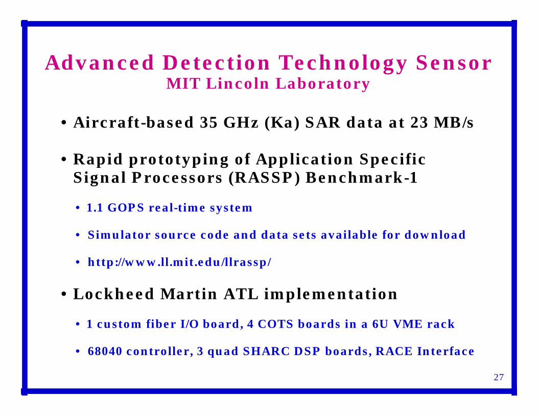
• Aircraft-based 35 GHz (Ka) SAR data at 23 MB/s

• Rapid prototyping of Application Specific Signal Processors (RASSP) Benchmark-1

27

Advanced Detection Technology SensorMIT Lincoln Laboratory

• 1.1 GOPS real-time system

• Simulator source code and data sets available for download

• http://www.ll.mit.edu/llrassp/

• Lockheed Martin ATL implementation

• 1 custom fiber I/O board, 4 COTS boards in a 6U VME rack

• 68040 controller, 3 quad SHARC DSP boards, RACE Interface

SAR Processor Block Diagram• Video-to-baseband (demodulate and FIR filter)

• Range compression (weighting and FFT)

• Azimuth compression (FFT, multiply, and FFT-1)

• Three independent channels (polarizations)

28

144 MOPS

Video-to-baseband

209 MFLOPS 725 MFLOPS

AzimuthCompression

Pulse data23 MB/sec

RangeCompression

• Collaboration with UT Center for Space Research

SensorData

Image data34 MB/sec

ThreePolarizations

Conclusion

29

• Bounded Process Network model extended withfiring thresholds from Computation Graphs

• Provides correctness and determinate execution

• Naturally models parallelism in system

• Models overlapping algorithms on continuous streams of data

• Multiprocessor workstation implementataion

• Designed for high-throughput data streams

• Native signal processing on general-purpose processors

• SMP operating systems, real-time lightweight POSIX Pthreads

• Low-overhead, high-performance and scalable

• Reduces implementation time and cost

Future Work

30

• Case studies

• Complete SAR processor case study

• Multimedia applications

• Multichannel image restoration

• Framework enhancements and extensions

• Integration with rapid prototyping tools

• Multiple identical channels – busses of streams

• Multiple executions of a program graph

• Formal analysis of framework properties

• Verify that the use of thresholds preserves PN properties

• Analyze the consequences and limitations of multiple executions

PublicationsG. E. Allen, B. L. Evans, and D. C. Schanbacher, “Real-Time Sonar

Beamforming on a Unix Workstation Using Process Networks and POSIX

Pthreads”, Proc. IEEE Asilomar Conf. on Signals, Systems, and

Computers, Nov. 1-4, 1998, Pacific Grove, CA, invited paper, vol. 2, pp.

1725-1729.

G. E. Allen and B. L. Evans, “Real-Time High-Throughput Sonar

Beamforming Kernels Using Native Signal Processing and Memory

Latency Hiding Techniques”, Proc. IEEE Asilomar Conf. on Signals,

Systems, and Computers, Oct. 25-28, 1999, Pacific Grove, CA, submitted.

G. E. Allen and B. L. Evans, “Real-Time Sonar Beamforming on a Unix

Workstation Using Process Networks and POSIX Threads”, IEEE

Transactions on Signal Processing, accepted for publication.

33

Time-Domain Beamforming

b(t) = αi xi(t–τi)Σ

i = 1

M

b(t) beam outputi

xi(t) ith sensor output

τi ith sensor delay

αi ith sensor weight

• Delay-and-sum weighted sensor outputs

• Geometrically project the sensor elements onto a line to compute the time delays

-20 -15 -10 -5 0 5 10 15 20

-5

0

5

10

15

20

Projection for a beam pointing 20° off axis

x position, inches

20°

sensor elementprojected element

Thread Pools• A boss / worker model for threads

• A fixed number of worker threads are created at initialization time

• The boss inserts work requests into a queue

• Workers remove and process the requests

Boss thread

Pool of worker threads

Queue ofwork requests

Process Network Nodes• Full system: 4 GFLOPS of computation

• A single processor (thread) cannot achieve real-time performance for any one node

• Use a thread pool to allow each node to execute in real-time (data parallelism)

• The number of worker threads is set as processing performance dictates

• For this implementation:

• The vertical beamformer node uses 4 worker threads

• Each horizontal beamformer node uses 4 worker threads