a fully actuated tail propulsion system for a biomimetic...
TRANSCRIPT

A Fully Actuated Tail Propulsion System for a
Biomimetic Autonomous Underwater Vehicle
A Thesis submitted in partial fulfilment of the requirement for the Degree of Doctor of Philosophy
Aerospace Sciences
School of Engineering University of Glasgow
By Ahmad Naddi Ahmad Mazlan
January 2015
© Ahmad Naddi Ahmad Mazlan, 2015

i
Author’s Declaration I declare that this thesis is my own work and that due acknowledgement has been given by
means of complete references to all sources from which material has been used for this
thesis. I also declare that this thesis has not been presented elsewhere for a higher degree.
Ahmad Naddi Ahmad Mazlan
January 2015

ii
Abstract In recent years that has been a worldwide increase in the utilisation of Autonomous
Underwater Vehicles (AUVs) for many diverse subsea applications. This has given rise to
an increase in the research and development of these vehicles, with a particular focus on
extending operational capability and longevity. Consequently, this activity has resulted in
the design of many different types of AUVs that employ a variety of different propulsion
and manoeuvring mechanisms. One particular area that has yielded promising results
involves the vehicles designs that are biologically inspired or biomimetic. This class of
AUV replicates the anatomical features of aquatic species in order to exploit some of the
benefits associated with this type of swimming e.g. higher efficiency at low speeds,
improved manoeuvrability. The study presented in this thesis considers the design and
performance analysis of a unique biomimetic AUV design based on the physiology of an
adult Atlantic salmon. This vehicle, called RoboSalmon, is equipped with a multiple
jointed, fully actuated tail that is used to replicate the undulatory swimming gait of a real
fish. The initial stage of this design process involves the development of a mathematical
model to describe the fusion of the dynamics and electro-mechanics of this vehicle. This
model provides the design specifications for a prototype vehicle, which has been used in
water tank trials to collect data. Forward swimming and manoeuvring experiments, e.g.
cruise in turning and turning circle swimming patterns, have been conducted for
performance analysis and validation purposes. This part of the study has illustrated the
relationship between the vehicle surge velocity, tail amplitude and tail beat frequency. It
was found that the maximum surge velocity has been measured at 0.143 ms-1. Also, the
vehicle has been shown to accomplish turning circle manoeuvres with turning radius just
over the half of its body length. The final stage of this study involved the design of a
heading control system, which changes the course of the vehicle by altering the tail
centreline. This study allowed the course changing performance of the vehicle to be
analysed. Furthermore, a line of sight guidance system has been used to navigate the
vehicle through a multiple waypoint course in order to show autonomous operation within
a simulated environment. Moreover, the vehicle has demonstrated satisfactory performance
in course changing and tracking operations. It is concluded that the RoboSalmon
biomimetic AUV exhibits higher propulsive efficiency and manoeuvrability than propeller
based underwater vehicles at low speeds. Thus the results of this study show that
mimicking biology can improve the propulsive and manoeuvring efficiencies of AUVs.

iii
Acknowledgement First and foremost, my appreciation and thanks go to my supervisor Dr Euan McGookin
for his endless guidance, assistance and patience throughout the course of my study. His
contribution is highly appreciated particularly in guiding me through this challenging
experience not just to complete this research but to be a better researcher.
I am truly and deeply indebted to numerous technical staff in the James Watt and Rankine
Building, especially John Kitching and John McCulloch for helping me with the
fabrication work as well sharing their technical knowledge. Also, I have to record my deep
sense of appreciation to my friends whom had contributed either directly or indirectly to
my study and supported me through the difficult times.
Finally and most of all, I would like to thank my parents, Ahmad Mazlan Osman and
Zainun Mohamad Yusoff, and both my sisters, Nadiatul Azra and Natrah Amira for the
immense amounts of patience, support, encouragement and dua’. Without their
contributions this thesis would not have been possible.

iv
Table of Contents Table of Contents
Author’s Declaration .............................................................................................................. i
Abstract ................................................................................................................................. ii
Acknowledgement ................................................................................................................ ii
Table of Contents ................................................................................................................. iv
List of Figures .................................................................................................................... viii
List of Tables ..................................................................................................................... xiv
1 Introduction ......................................................................................................................... 1
Preface ................................................................................................................... 1 1.1
Research Motivation .............................................................................................. 3 1.2
Atlantic Salmon - Subcarangiform ........................................................................ 4 1.3
Aims & Objectives ................................................................................................ 5 1.4
Contribution of Research ....................................................................................... 5 1.5
Thesis Structure ..................................................................................................... 6 1.6
2 Literature Review ................................................................................................................ 8
Introduction ........................................................................................................... 8 2.1
Conventional Underwater Vehicle ........................................................................ 9 2.2
Biomimetic Underwater Vehicles ....................................................................... 15 2.3
Biomimetic Underwater Vehicle Prototypes ....................................................... 17 2.4
RoboTuna ..................................................................................................... 17 2.4.1
RoboPike ...................................................................................................... 19 2.4.2
GhostSwimmer & BIOSwimmer ................................................................... 19 2.4.3
Vorticity Control Unmanned Undersea Vehicle (VCUUV) ........................ 19 2.4.4
Essex Robotic Fish ....................................................................................... 21 2.4.5
PF and UPF Series ....................................................................................... 21 2.4.6

v
RoboSalmon V2 ............................................................................................ 22 2.4.7
UWFUV ....................................................................................................... 23 2.4.8
SPC Series .................................................................................................... 24 2.4.9
Pearl Arowana .............................................................................................. 25 2.4.10
NAF-II and NEF-II ...................................................................................... 26 2.4.11
Summary .............................................................................................................. 27 2.5
3 RoboSalmon Design .......................................................................................................... 29
Introduction ......................................................................................................... 29 3.1
Hardware Design ................................................................................................. 32 3.2
Tail Section .................................................................................................. 33 3.2.1
Body Section ................................................................................................ 36 3.2.2
Electrical Systems ............................................................................................... 39 3.3
Electronic Systems in the Body Section ...................................................... 40 3.3.1
Electronic Systems in the Tail Section ........................................................ 46 3.3.2
Summary .............................................................................................................. 49 3.4
4 Mathematical Modelling ................................................................................................... 50
Introduction ......................................................................................................... 50 4.1
Multi-rate Simulation .......................................................................................... 52 4.2
State Space Modelling ......................................................................................... 53 4.3
Reference Frames ................................................................................................ 54 4.4
Vehicle Kinematic ............................................................................................... 56 4.5
Vehicle Dynamics................................................................................................ 57 4.6
Rigid Body Dynamics .................................................................................. 57 4.6.1
Mass and Inertia Matrix ............................................................................... 59 4.6.2
Coriolis and Centripetal Matrix ................................................................... 59 4.6.3
Hydrodynamic Forces and Moments ........................................................... 60 4.6.4
Added Mass Terms ...................................................................................... 60 4.6.5
Hydrodynamic Damping .............................................................................. 63 4.6.6

vi
Restoring Forces and Moments .................................................................... 65 4.6.7
Tail Propulsion System ........................................................................................ 67 4.7
Tail Kinematics ............................................................................................ 67 4.7.1
Denavit Hartenberg Representation ............................................................. 69 4.7.2
DC Motor Model .......................................................................................... 73 4.7.3
Gear Ratio .................................................................................................... 75 4.7.4
DC Motor Position Control .......................................................................... 76 4.7.5
Thrust Generation ........................................................................................ 77 4.7.6
RoboSalmon State Space Equations .................................................................... 80 4.8
Model Validation ................................................................................................. 81 4.9
Analogue Matching ...................................................................................... 82 4.9.1
The Integral Least Squares ........................................................................... 84 4.9.2
Summary .............................................................................................................. 84 4.10
5 Forward Swimming ........................................................................................................... 85
Introduction ......................................................................................................... 85 5.1
Data Collection .................................................................................................... 85 5.2
Laboratory Equipment ................................................................................. 86 5.2.1
Experimental Procedure ............................................................................... 87 5.2.2
Image Processing ......................................................................................... 89 5.2.3
Sensor Data Post Processing ........................................................................ 90 5.2.4
Forward Swimming ............................................................................................. 93 5.3
Strouhal Number ........................................................................................ 105 5.3.1
Power ......................................................................................................... 109 5.3.2
Recoil Motion ............................................................................................ 115 5.3.3
Actuated Head ................................................................................................... 118 5.4
Summary ............................................................................................................ 120 5.5
6 Manoeuvring Swimming ................................................................................................. 122
Introduction ....................................................................................................... 122 6.1

vii
Tail Manoeuvring System ................................................................................. 123 6.2
Cruise in Turning ............................................................................................... 124 6.3
Zig-zag Manoeuvre............................................................................................ 137 6.4
Power Consumption .......................................................................................... 139 6.5
Summary ............................................................................................................ 141 6.6
7 Autonomous Control & Guidance .................................................................................. 143
Introduction ....................................................................................................... 143 7.1
Heading Controller ............................................................................................ 143 7.2
Reference Heading Model ................................................................................. 144 7.3
PID Heading Controller ..................................................................................... 146 7.4
Integrator Windup.............................................................................................. 147 7.5
PID heading controller performance .......................................................... 148 7.5.1
Sliding Mode Heading Controller ..................................................................... 154 7.6
Sliding Mode Heading Controller Performance ........................................ 159 7.6.1
Line of Sight (LOS) ........................................................................................... 160 7.7
Summary ............................................................................................................ 167 7.8
8 Discussion, Conclusions & Further Work ...................................................................... 169
Discussion and Conclusions .............................................................................. 169 8.1
Further Work ..................................................................................................... 173 8.2
Modelling and Simulation .......................................................................... 173 8.2.1
RoboSalmon System Improvement ............................................................ 174 8.2.2
References .......................................................................................................................... 175
Appendix A ........................................................................................................................ 202
Appendix B ........................................................................................................................ 207
Appendix C ........................................................................................................................ 208
Appendix D ........................................................................................................................ 211

viii
List of Figures Figure 2.1: SeaOtter Mk II AUV with rectangular hull shape ............................................. 10
Figure 2.2: Autonomous Benthic Explorer (ABE) that has multihull vehicle shape ........... 10
Figure 2.3: A 12” diameter Bluefin Robotic AUV .............................................................. 11
Figure 2.4: Swimming modes associated with (a) BCF propulsion and (b) MPF propulsion.
The shaded areas contribute to the thrust generation ........................................................... 16
Figure 2.5: RoboTuna .......................................................................................................... 18
Figure 2.6: VCUUV system layout ...................................................................................... 20
Figure 2.7: RoboSalmon vehicle with tendon drive propulsion system ............................... 23
Figure 2.8: The University Washington fin-actuated underwater vehicle ........................... 24
Figure 2.9: Three link tail mechanism of a NAF-II prototype ............................................. 26
Figure 2.10: NEF-II with 5 DOF structure .......................................................................... 27
Figure 3.1: BCF swimming movements (a) anguilliform (b) subcarangiform
(c) carangiform (d) thunniform mode .................................................................................. 30
Figure 3.2: RoboSalmon V3.0 (a) actual (b) digital prototype ............................................. 33
Figure 3.3: Tail section ........................................................................................................ 34
Figure 3.4: (a) Atlantic salmon (Salmo salar) (b) Caudal Fin used on prototype tail
propulsion system ................................................................................................................ 35
Figure 3.5: Robosalmon with (a) Silicone rubber skin (b) Latex rubber skin...................... 36
Figure 3.6: Fiberglass body and tail cover ........................................................................... 37
Figure 3.7: Pectoral fins ....................................................................................................... 38
Figure 3.8: Body section ...................................................................................................... 38
Figure 3.9: Electrical system schematic diagram ................................................................. 39
Figure 3.10: Upper enclosure (a) circuit board (b) block diagram ...................................... 41
Figure 3.11: Lower enclosure (a) circuit board (b) block diagram ...................................... 45
Figure 3.12: Tail motor drive (a) circuit board (b) block diagram ...................................... 47
Figure 4.1: Multiple individually actuated tail joint (red box) ............................................ 51

ix
Figure 4.2: Multi-rate simulation structure .......................................................................... 53
Figure 4.3: Body fixed and Earth fixed reference frames .................................................... 55
Figure 4.4: (a) Prolate Ellipsoid model with semi-axes a,b and c (b) Projection of Prolate
Ellipsoid shape (red) to vehicle model ................................................................................. 62
Figure 4.5: Drag calculation for caudal fin .......................................................................... 64
Figure 4.6: Fish kinematics using travelling wave equation ................................................ 68
Figure 4.7: Multi-joint tail configuration ............................................................................. 69
Figure 4.8: Fish kinematics using RoboSalmon tail assembly with circle indicate joints ... 73
Figure 4.9: Schematic model of revolute joint. θm is the angular position of the motor (rad)
and θL is the load position of the motor ............................................................................... 75
Figure 4.10: Motor block diagram with PID controller ....................................................... 76
Figure 4.11: PID controller with saturation block. .............................................................. 77
Figure 4.12: (a) Top view of the outline of a RoboSalmon swimming motion in time (b)
The red box in Figure 4.12(a) is redrawn on a larger scale with the broken arrow indicates
the instantaneous velocity vector of the caudal fin tip has been resolved into components k
and w .................................................................................................................................... 79
Figure 4.13: The analogue matching validation technique for RoboSalmon forward
swimming. The blue trace is the experimental data and red trace for simulation data ........ 82
Figure 4.14: The pitch and yaw angular velocities graph in Figure 4.13 is redrawn with the
blue trace is the experimental data and red trace for simulation data. ................................. 83
Figure 5.1: Experimental setup ............................................................................................ 86
Figure 5.2: Schematic image of laboratory equipment ........................................................ 87
Figure 5.3: Flowchart of experimental procedure ................................................................ 88
Figure 5.4: Image processing steps (a) image captured by the camera (b) conversion to
binary image with the object (white) and background (black) (c) Image undergo
morphological operations (d) the centre of the red blob is indicate by (+) yellow .............. 89
Figure 5.5: Selection of on-board sensors post processing .................................................. 91
Figure 5.6: Image post processing ....................................................................................... 92
Figure 5.7: Vehicle path for forward swimming .................................................................. 93

x
Figure 5.8: Data obtained from image processing (a) vehicle’s x-y position (b) surge and
sway ..................................................................................................................................... 94
Figure 5.9: Data obtained from sensors on-board the vehicle ............................................. 96
Figure 5.10: Relationship between surge velocity and frequency for all forward swimming
experiments corresponding to the tail beat amplitude of (a) 0.05 m (b) 0.10 m (c) 0.15 m
and (d) 0.20 m ...................................................................................................................... 98
Figure 5.11: Estimation of vehicle surge velocities for 0.10 m tail beat amplitude with tail
beat frequencies of 0.5 Hz, 1 Hz, 1.5 Hz, 2 Hz, 2.5 Hz and 3 Hz........................................ 99
Figure 5.12: Actuator angular position respond based on various tail beat amplitudes when
operates at 1 Hz tail beat frequency. The circles indicate the final angular position on each
step with the tail beat amplitude of 0.05 m (yellow), 0.10 m (blue), 0.15 m (red) and
0.20 m (green) .................................................................................................................... 101
Figure 5.13: Simulated vehicle surge velocities for 1 Hz tail beat frequency with tail beat
amplitude of 0.05 m, 0.10 m, 0.15 m and 0.20 m .............................................................. 103
Figure 5.14: Surge velocity relates to tail beat amplitude and frequency. The saturated
values are replaced with the simulation values .................................................................. 104
Figure 5.15: 3D Plot relationship between surge velocity, tail beat amplitude and tail beat
frequency. (a) experimental values (grey) (b) saturated values in experimental values are
replaced with simulation values (mesh plot) ...................................................................... 105
Figure 5.16: Comparison of swimming speed relates to frequency. Estimated range of
optimal speed of Atlantic Salmon (blue dashed lines), Atlantic Salmon (green points),
RoboSalmon (red points) with extrapolated data (red dashed lines) .................................. 107
Figure 5.17: Strouhal number vs. frequency for the RoboSalmon (a) experimental (non-
saturated and saturated) (b) non-saturated and simulated values ....................................... 108
Figure 5.18: The RoboSalmon tail current (top), voltage (middle) and power consumption
(bottom) .............................................................................................................................. 110
Figure 5.19: Electrical power consumption ....................................................................... 111
Figure 5.20: Estimation of real fish swimming power relates to the swimming speed ..... 112
Figure 5.21: RoboSalmon swimming power output ........................................................... 113
Figure 5.22: RoboSalmon propulsion efficiency ................................................................ 114

xi
Figure 5.23: Quantitative comparison of magnitude in roll, pitch and yaw angular
velocities. The tail beat amplitudes are indicated by the blue points (0.05 m), red points
(0.10 m), green points (0.15 m) and magenta point (0.20 m) ............................................ 116
Figure 5.24: Quantitative comparisons of magnitude in roll, pitch and yaw angular
position. The tail beat amplitudes are indicated by the blue points (0.05 m), red points
(0.10 m), green points (0.15 m) and magenta point (0.20 m) ............................................ 117
Figure 5.25: Actuated head configuration -18º (left), 0º (centre) and +18º (right) ............ 118
Figure 5.26: XY Trajectory with and without actuated head deflection ............................ 119
Figure 6.1: Tail deflection angle (a) left (b) centre (c) right .............................................. 124
Figure 6.2: Turning circle test ............................................................................................ 125
Figure 6.3: RoboSalmon path trajectory for configuration of 0.10 m tail beat amplitude,
1 Hz tail beat frequency and -50° tail deflection angle ...................................................... 126
Figure 6.4: Experimental values of vehicle turning radius for cruise in turning ............... 127
Figure 6.5: Comparison between experiment and simulation data of vehicle turning radius
for cruise in turning for tail beat frequency of 1 Hz and 0.10 m........................................ 128
Figure 6.6: Experimental values of surge velocity vs tail deflection angle with tail beat
amplitude and frequency of (a) 0.10 m, 0.5 Hz (b) 0.10 m. 1.0 Hz (c) 0.15 m, 0.5 Hz
(d) 0.15 m, 1.0 Hz .............................................................................................................. 129
Figure 6.7: (a) Roll and (b) yaw rate for turning manoeuvre ............................................. 130
Figure 6.8: Average roll and yaw rates relate to tail deflection angle ............................... 131
Figure 6.9: Experimental measured values of vehicle turning radius, RT for both direction
of tail deflection angle, δT .................................................................................................. 132
Figure 6.10: Turning circle for a 90º tail deflection angle where (1) start, (2) middle and
(3) final position. ................................................................................................................ 133
Figure 6.11: Turning circle parameters for the vehicle with tail deflection angle of 90°
(experiment) ....................................................................................................................... 134
Figure 6.12: The tail deflection angle configuration of 90°. (a) Yaw rate (blue) and average
yaw rate (red) (b) vehicle speed (blue) and average speed (red) ....................................... 135
Figure 6.13: Simulation result of turning circle parameters for the vehicle with tail
deflection angle of 90° ....................................................................................................... 136

xii
Figure 6.14: Simulated values of vehicle turning circle with ±10º, ±20º, ±30º, ±40º, ±50º,
±60º, ±70º, ±80º and ±90º tail deflection angles ................................................................ 137
Figure 6.15: Characteristic of zig-zag manoeuvre ............................................................. 138
Figure 6.16: Simulated the vehicle performance in 20º/20º zig-zag manoeuvre. The vehicle
heading is indicates by blue line and tail deflection angle is indicates by red line ............ 138
Figure 6.17: The vehicle zigzag manoeuvre for various tail beat configurations .............. 139
Figure 6.18: Comparison of vehicle power consumption for various tail deflection angles
with 0.10 m tail beat amplitude and two tails beat frequencies (0.5 Hz and 1 Hz) ........... 140
Figure 7.1: Vehicle heading control system ....................................................................... 144
Figure 7.2: Heading reference model for 90º ..................................................................... 145
Figure 7.3: Comparison of vehicle control performance when applied with or without
filtered command ............................................................................................................... 146
Figure 7.4: Back Calculation anti-windup PID controller ................................................. 148
Figure 7.5: The vehicle (a) heading with respect to earth reference frame (b) path trajectory
for 30° heading indicated by the red dots .......................................................................... 149
Figure 7.6: The Vehicle performance in terms of heading and tail deflection angle with
desired heading of -30º (Experiment) ................................................................................ 150
Figure 7.7: The Vehicle performance in terms of heading and tail deflection angle with
desired heading of 30º (Experiment) .................................................................................. 151
Figure 7.8: Heading errors for 30º and -30º heading angles .............................................. 152
Figure 7.9: The Vehicle performance in terms of heading and tail deflection angle with
desired heading of -60º (Experiment) ................................................................................ 153
Figure 7.10: Heading errors for -60º heading angles ......................................................... 153
Figure 7.11: Vehicle heading motion based on change in tail centreline for PID controller.
The vehicle is commanded to 60º, 0º and 60º headings ..................................................... 154
Figure 7.12: Vehicle heading motion based on change in tail centreline for sliding mode
controller. The vehicle is commanded to 60º, 0º and 60º headings ................................... 160
Figure 7.13. Autonomous guidance and heading control system ...................................... 161
Figure 7.14: Waypoint and acceptance radius ................................................................... 161
Figure 7.15: Line of sight guidance system for waypoint tracking with PID controller ... 163

xiii
Figure 7.16: PID controller performance on vehicle tracking angle and tail centreline .... 164
Figure 7.17: PID controller performance on the tail centreline relates to motor current ... 165
Figure 7.18: Line of sight guidance system for waypoint tracking with sliding mode
controller ............................................................................................................................ 166
Figure 7.19: Sliding mode controller performance on vehicle tracking angle and tail
centreline ............................................................................................................................ 166
Figure 7.20: Sliding mode controller performance on the tail centreline relates to motor
current ................................................................................................................................ 167

xiv
List of Tables Table 2.1. AUV hull shape ................................................................................................... 10
Table 3.1: Sensor specification parameters .......................................................................... 43
Table 3.2: Electronic components distribution in tail section .............................................. 48
Table 4.1: Notation used for marine vehicles ...................................................................... 55
Table 4.2: RoboSalmon tail parameter table ........................................................................ 70
Table 5.1: Surge velocity relates to tail beat amplitude and frequency ............................... 97
Table 5.2: Average vehicle surge velocity respect to different tail beat frequency ........... 100
Table 5.3: Desired motor angular position for one cycle ................................................... 102
Table 5.4: Simulated motor angular position for one cycle ............................................... 102
Table 5.5: Average vehicle surge velocity respect to different tail beat amplitude ........... 103
Table 5.6: Velocities comparison between actuated and stationary head .......................... 119
Table 6.1: Turning circle characteristic ............................................................................. 134
Table 6.2: Experimental values of power consumption for various tail deflection angles for
tail beat amplitude of 0.10 m and 1 Hz tail beat frequency ............................................... 140
Table 7.1: Sliding Mode heading controller parameters .................................................... 158
Table 7.2: Waypoints ......................................................................................................... 162

Introduction
1
1
Introduction
Preface 1.1
Deep sea exploration is considered to be a challenging task due to the complexity and
hazardous nature of the underwater environment. The growing industry in unmanned
underwater vehicles has renewed the attention of scientist and researchers to overcome the
challenging scientific and engineering problems associated with the unstructured and
hazardous underwater environment. This includes the study of vehicle design, actuator
specification and development of motion control algorithms which have been reported in
the past decades (Molnar, et al., 2007; Zhu & Sun, 2013). The unmanned underwater
vehicle (UUV) has been widely used in sea bottom exploration, repairing, surveying,
inspection, oil and gas exploration, mine countermeasure, search & rescue and gathering
scientific data (Tan, et al., 2007; Akcakaya, et al., 2009; Seto, et al., 2013; Zhu & Sun,
2013).
Nonetheless, the UUV usefulness is not limited to deep sea applications. Numbers of UUV
applications can be applied in shallow water environments (e.g. river, lake) for inspection
and collecting samples task. This has led to concept designs of much smaller scale of
UUVs, low cost fabrication and operation (Bellingham, et al., 1994; Wang, et al., 2008a).
Generally, underwater vehicle classification can be divided into two major categories;
manned underwater vehicles (MUVs) and unmanned underwater vehicles (UUVs). The
remotely operated vehicles (ROVs) and autonomous underwater vehicles (AUVs) fall into
the UUV category (Blidberg, 2001; Christ & Wernli Sr, 2014).
One of the most popular category class is the ROV as the name suggests is tethered with
umbilical cable and remotely operated by pilot commands from the surface (Christ &
Wernli Sr, 2014). Moreover, the power of the vehicle can be on-board, off-board or a
hybrid of both. In an off-board condition, the power is supplied to the ROV using a tether.
Elvander & Hawkes (2012) stated that ROVs are used to replace divers at depths or within

Introduction
2
higher risk environments. The human intervention in ROVs operations makes them
suitable for operations that require complex manipulations at great depth (Chadwick, 2010;
From, et al., 2014)
The unmanned underwater vehicle has been involved in a number of underwater
archaeological surveys where ROVs have been used to investigate the wrecks of RMS
Titanic in 1986 and German battleship Bismarck in the summer of 1989 (Ballard, 1993).
The Jason Jr., a small ROV developed by the Woods Hole Oceanographic Institution was
deployed to explore the interior of the Titanic in conjunction with the deep diving
submarine Alvin (Yoerger & Slotine, 1991). The Jason Jr. operates under the guidance
from an operator inside Alvin through fibre optic cables. This capability allow scientists to
explore and photograph wreck area that would be too dangerous for Alvin and divers to
venture (Sellers, 2010).
Another type of UUV is the AUV, an untethered underwater vehicle which Tan, et al.
(2007) described as “a free swimming vehicle of high autonomy”. This type of vehicle is
capable of performing missions without human intervention. The freedom of movement
provide advantages over ROVs where increase the operating range which make the AUVs
suitable for inspection and surveying (Akcakaya, et al., 2009; Chadwick, 2010; Roper, et
al., 2011) and the operating cost also can be reduced as the support vessel can be operated
in multiple sites (Roper, et al., 2011). However, it can be noted that this operating range is
limits on board power source. In addition, since it does not need supervision, it is required
to be programmed in advance. It returns to a pre-programmed location once the mission is
completed where the vehicle and its data are retrieved.
An AUV can also be used to complement the ROV missions and vice versa. One of the
most useful applications of ROV and AUV technologies can be seen in search and rescue
missions which have involved the recovery of downed aircraft such as the wreckage search
of Swissair Flight 111 (Petersen, 2007), Air France 447 (Wise, 2011) and with the recent
search for the missing Malaysia Airlines Flight 370 (Smith & Marks, 2014). Smith &
Marks (2014) stated that the Bluefin Robotics AUV, named Bluefin-21 is among the tools
deployed to hunt for the missing aircraft. Since the exact location of the MH370 crash site
is not known, it makes the search process particularly tricky with uncertain measured
depths of sea level needed to be covered. The AUV has the capability of mapping the sea
floor at a depth of 4500 m below sea level through the use of sonar. However, up until now
the search has been unsuccessful which has caused the search to be expanded and new

Introduction
3
underwater vehicles to be deploy to join the Bluefin-21. One of the suggested vehicles is
the REMUS 6000 (Sanchez, 2014) which is similar to Bluefin-21 but can operate at depths
of 6000 m. Previously, the REMUS 6000 aided in the search and discovery of the
wreckage of Air France Flight AF447 at the bottom of the Atlantic Ocean (Purcell, et al.,
2011; Wise, 2011).
Research Motivation 1.2
Nowadays, several abilities such as travel at low and high speed, longer mission duration,
manoeuvrability and navigation purpose have become essential to underwater vehicles.
Existing AUVs propeller based systems are designed to work efficiently for a mission (e.g.
mapping, surveying) that required cruising at high speed. However, in certain applications
the propeller based system appears to be inefficient. It has been noted that this system has
poor manoeuvring performance (i.e. does not allow it to manoeuvre at low speed and has
large turning circle). A large amount of research has been done into optimizing the
propeller based system for various applications (e.g. azimuth thruster). This includes
configuring multiple thrusters around the vehicle body to allow it to manoeuvre at low
speed. Conversely, this configuration increases the vehicle power usage.
Researchers (Liu, et al., 2005; Yu, et al., 2010; Liu, et al., 2014) found that a more efficient
propulsion system is necessary to produce better vehicle performance. Researchers have
tended to look to nature as an inspiration for their design where the biomimetic propulsion
system has been considered as an alternative to propeller based system. The term
biomimetic or biomimicry represents the imitation of nature’s methods, mechanisms and
processes into man-made systems (Bar-Cohen, 2006). In recent years, people have become
more focused on the efficient swimming capabilities of fish and the potential benefits that
can be transferred to marine vehicle design by mimicking or being inspired by biological
based swimming. As examples fish such as pike and yellowfin tuna that can swim at high
speed with high level of efficiency and the eel that manoeuvres skilfully within confined
spaces (Triantafyllou & Hover, 2003). Moreover, this includes the real fish
manoeuvrability ability such as performing a rapid turn for catching prey and avoiding
obstructions (Fish, 1997; Guo & Wang, 2008).
This versatile range of swimming abilities has inspired researchers to improve the
performance of current autonomous underwater vehicles by implementing biomimetic
propulsion systems that replicate the motion of the fish. The investigations into biomimetic

Introduction
4
systems have provided significant insights into both theory and application of robotics in
recent years which can lead to increases in vehicle efficiency and manoeuvrability (Liu, et
al., 2005; Yu, et al., 2007; Watts, 2009). Therefore, in the context of this study, the idea is
to mimic the nature of real fish swimming to replace the conventional propeller based
system that is used extensively in underwater vehicles applications.
Atlantic Salmon - Subcarangiform 1.3
Anderson & Chhabra (2002) indicated that there is trade off existence between speed and
manoeuvrability in types of fish where the design choice depends on researchers to select
the most desirable attributes to mimic in their designs. In this study, a biomimetic
underwater vehicle has been developed with multi jointed tail that imitates Atlantic
salmon. The Atlantic salmon has subcarangiform locomotion that approximately 2/3 to 1/2
of their body involved in the propulsive wave for forward motion (Hoar & Randall, 1978).
This genus of fish has been chosen because it exhibits several beneficial attributes. The
first of these is that salmon swimming performance provides both reasonably fast
propulsion and efficient manoeuvring capabilities.
Generally the Atlantic salmon can be found in several locations across Europe, North
America and United Kingdom where the majority of the European market is dominated by
Norwegian and United Kingdom industries (Mora, et al., 2011). Mora, et al. (2011) stated
that about half of total stock is from Norway and another quarter from the United Kingdom
i.e. Scottish rivers (Conservation of Atlantic Salmon in Scotland Project, 2010). This
indicates the importance of salmon fisheries sector contributions towards the Scottish
economy where salmon has become Scotland’s number one food export (Scottish Salmon
Producers' Organisation, 2012).
Another key attribute is that salmon have amazing navigation capabilities which is
considered to be one of the marvels of nature where they precisely return to their home
river even after migrating across thousands of miles of open water (Young, 1962;
Verspoor, et al., 2007). Moreover, the size of an Atlantic salmon allows an electronic
circuit and sensors to sufficiently occupy the space of a prototype hull. Moreover, it is
found the manageable size of the Atlantic salmon enables it to be experimenting in smaller
water tank compared to other larger vehicle that require special testing facilities and a team
of operators (Watts, 2009).

Introduction
5
Aims & Objectives 1.4
The work carried out in this research is aimed to investigate the potential benefits of
utilising a biomimetic propulsion system for the underwater vehicles design. In order for
this aim to be achieved, several objectives must be met first. The objectives for this
research are described below:
1. Develop a mathematical model to assist with the understanding of the dynamics of the
biomimetic underwater vehicle and to estimate the performance of the prototype
hardware.
2. Develop fishlike motion control algorithms for the biomimetic underwater vehicle.
3. Analyse the biomimetic propulsion system swimming performance by undergo several
physical trials.
4. Validate the prototype hardware performance with data obtained from model using
qualitative and quantitative measurement.
5. Implement heading and guidance control system for path tracking.
Contribution of Research 1.5
The contributions of this research can be summarized as follows:
1. Development of a fully actuated biomimetic AUV based on fish swimming
2. The hydrodynamics of the biomimetic AUV is analysed using a mathematical model.
The model has been developed based on the conventional marine vessels where there
is significant difference in technique to represent the propulsion system mimicking
real fish undulation motion.
3. Control algorithms altering tail centreline has been presented in order for the vehicle
to have manoeuvring capability.
4. Use of a validated model to develop an autonomous guidance control system for the
vehicle.
Introduction
6
Thesis Structure 1.6
The study of a fully actuated tail propulsion system implemented on an autonomous
underwater vehicle is carried out in this thesis as outlined below:
Chapter 2 presents an overview of existing research in areas related to this work. It consists
of an overview of conventional underwater vehicles and their applications. This followed
by lists of numbers of biomimetic vehicle designs that has been developed in last decade to
investigate the performance of fish like swimming motion.
Chapter 3 presents the design and development of a fully actuated version of a
RoboSalmon prototype. The relevant aspects concerning fish swimming motion are
discussed to provide a biological basis for the tail design. The challenges in both
mechanical and electronic system design are discussed in detail.
The development of mathematical model describing the dynamic behaviour of a
biomimetic underwater vehicle is discussed in Chapter 4. This mathematical model is used
to determine the kinematic and dynamic performance of the vehicle. It is modelled using
the conventional marine vessel techniques with several modifications taken into accounts
especially the way it produces thrust for forward movement. This chapter also includes
details of the experimental laboratory setup used to test of the RoboSalmon vehicle and
collect physical data for validating the mathematical model validation process.
Chapter 5 describes the RoboSalmon experimentation and simulation outcomes for the
forward motion. It involved varying the tail beat parameters that consist of tail beat
amplitude and frequency. The effect of these parameters towards the vehicle surge velocity
has been analysed. Followed by the discussion on the characteristic of the recoil motion
that affected by varying these tail beat parameters. An attempt to reduce the recoil motion
experienced by the vehicle is done by continuously utilizing the head motion is presented.
Finally, the vehicle performances in terms of propulsion efficiency and power consumption
have been measured.
Manoeuvring experimentation and simulation results are presented in Chapter 6 where the
vehicle is tested while performing a turning circle and zig-zag swimming pattern. This
involves varying the similar parameters used for forward swimming (i.e. tail beat
amplitude and frequency) with the addition of tail deflection angle. The symmetry of

Introduction
7
vehicle turning is tested by considering tail deflection angle on both sides of the tail
centreline.
Chapter 7 presents the design of RoboSalmon heading controller based on the Proportional
Integral Derivative (PID) and sliding mode control. The PID heading control has been
implemented on the vehicle in both simulation and experimentation while the sliding mode
only applied in simulation environment. These controllers are implemented in order to
control vehicle heading by altering the tail centreline with the heading tracking
performance of these heading controllers has been discussed and compared. Next step was
to introduce a guidance system in a form of line of sight to provide navigation ability for
the RoboSalmon vehicle. The vehicle was commanded to navigate through set of paths that
were made up from several waypoints.
Finally, Chapter 8 presents the conclusions that have been drawn from this study along
with a brief overview of how the results compare with the objectives set out at the start of
this thesis. This is followed by a section that discussed lists of suggestions and further
improvements that could be made on certain area of RoboSalmon in the future.

Literature Review
8
2
Literature Review
Introduction 2.1
This chapter aims to provide an overview of current AUV/UUV technologies. Propellers
thruster and control surface are commonly used for locomotion and manoeuvring for
underwater vehicles. The increase in research, commercial or military purposes generates
result an interest to develop a more efficient vehicle. As suggested earlier, the biomimetic
propulsion has been considered as an alternative to propeller driven propulsion. This
system is used to mimic fish tail like undulation motion for forward propulsion. It has been
argued that there are several advantages of a fish like propulsion system over a propeller
such as less noise, better manoeuvrability (Liu, et al., 2005), and relatively high energy
efficiency (Guo, et al., 1998; Rossi, et al., 2011a). Thus, the naturally evolved excellent
performance of fish has inspired researchers, engineers and scientists to apply biomimetic
technology to the design of underwater vehicles.
The field of biomimetic robotics is multi-disciplinary in nature where numerous different
subject areas such as mechanical, naval, electrical and electronics engineering are
involved. Therefore, it is important to acquire the relevant knowledge or ideas in modelling
and designing a biomimetic vehicle. Nonetheless, it is also necessary to discuss the
construction of conventional unmanned underwater vehicles in order to establish the
relevant requirements and limitations for the design of underwater vehicles. Therefore, this
chapter is divided into four further sections. Firstly, Section 2.2 presents the state of the art
in the design and construction of conventional underwater vehicles. Different approaches
in selecting types of actuator that involved in realizing the fish like motion are described in
Section 2.3. This is followed in Section 2.4 by a list of biomimetic swimming vehicles that
have been constructed for academic and commercial purposes. Finally Section 2.5 presents
concluding remarks drawn from this review of the current literature in this field of study.

Literature Review
9
Conventional Underwater Vehicle 2.2
As been mentioned in Chapter 1, UUV can be splits into ROVs and AUVs categories. Both
vehicles have demonstrated that they can operate well in underwater environment.
According to Christ & Wernli Sr (2014), the main difference between these vehicles is that
ROVs are tethered to the ship while AUVs are not. The power and communication is
supplies through this tethered cable and the ROV is operated by a pilot. On the other hand,
an AUV is a free moving vehicle that carries its own power supply (Blidberg, 2001). Both
types of vehicle possess different capabilities and limitation that make them better suited
certain applications than the other. However, this section will focus on autonomous
underwater vehicles, as this type of platform is most relevant to the research studies.
AUVs are a particular class of unmanned and self-contained UUVs that are able to
complete survey/sampling tasks as well as make navigational and tactical decision based
on inputs from the on board sensors (Bellingham, 2001; Chadwick, 2010). Thus, it can be
operated without supervision and need to be programmed ahead of time. AUVs have been
developed by many institutions with several vehicles having demonstrated their wide
ranging operational capabilities. They have been used in research, military and offshore
industry application where tasks such as surveying, pipe or cable inspection, surveillance
or reconnaissance, mine disposal and harbour patrolling are carried out (Lienard, 1990;
Corfield & Hillenbrand, 2002; Danson, 2002). Even though the applications and utilisation
of the AUV are varied, many have similar configuration and have basic subsystems
(Griffiths, 1999). These include subsystems for propulsion, navigation, mission
management, user interface, manipulator system and power storage.
The drag is an important element to be considered when designing an AUV hull shape and
Wang, et al.(2007) discussed that minimizing the effect of these elements helps to expand
the operational range, improve the load capability and increase efficiency. A wide variety
of AUV shapes and sizes have been designed (see Table 2.1) and ranging from torpedo
shape, laminar flow, streamlined rectangular style and multihull vehicles (Stevenson, et al.,
2007, 2009).

Literature Review
10
Table 2.1. AUV hull shape
Shape Vehicle
Torpedo Autosub (Millard, et al., 1997), Bluefin Robotic (Panish,
2009) and Remus (Allen, et al., 2000)
Laminar flow Early HUGIN vehicles (Marthiniussen, et al., 2004)
Streamlined
rectangular
Marius (Pascoal, et al., 1997) and Sea Otter MK-II (see Figure
2.1) (Atlas Elektronik GmbH, 2013)
Multihull vehicles Autonomous Benthic Explorer (ABE) (see
Figure 2.2) (German, et al., 2008)
Figure image has been removed due to Copyright restrictions
Figure 2.1: SeaOtter Mk II AUV with rectangular hull shape (Atlas Elektronik GmbH, 2013)
Figure image has been removed due to Copyright restrictions
Figure 2.2: Autonomous Benthic Explorer (ABE) that has multihull vehicle shape (Blidberg, 2001)

Literature Review
11
The earliest AUV was developed in 1800s and resemble a torpedo shape (Blidberg, 2001)
which is still the most popular choice of AUV shape configuration (Singh, et al., 1997;
Bellingham, 2001). Most torpedo shaped AUVs are propelled by single or dual fixed
propellers and manoeuvres through a set of actuated rudder and elevator control surfaces
(Eskesen, et al., 2009). This shape minimizes drag and as a consequence minimizes the
energy required for vehicle propulsion which then contributes to higher cruise efficiency.
Budiyono (2009) summarized that most commercially existing torpedo shape AUVs have
design speeds on average of 3 m/s.
Bluefin Robotics offers a wide range of AUVs that able to meet the requirement in
defence, commercial, and scientific demand (Panish, 2009; Goldberg, 2011). These AUV
products consists of Bluefin-9, Bluefin-12S, Bluefin-12D and Bluefin-21 classes of
torpedo shaped vehicles with three different diameters (i.e. 9”, 12” (see Figure 2.3), and
21”). According to Panish (2009), by using a core set of building blocks, the length of
vehicle can be fully configurable to meet the demands of the specific application, length
potentially range from 1 to 5 m.
Figure image has been removed due to Copyright restrictions
Figure 2.3: A 12” diameter Bluefin Robotic AUV (Panish, 2009)
Ducted tailcones propulsion design has been applied to these types of vehicles, it is used to
replace the extended dive planes and control fins that are common with many AUVs
(Panish, 2009). It is claimed that it provides exceptional propulsive efficiency, dynamic
stability, less maintenance, improved directional control in a compact and robust structure
(Bluefin Robotics, 2014). The Bluefin AUV can be deployed for shallow and deep water
survey applications where it is highly stable with extensively configurable tool, such as
side scan sonar, synthetic aperture sonar, and multibeam echo that can be used to produce
high quality measurement (Panish, 2009). This has been demonstrated by the high quality
imagery produced when integrate the Sonardyne International Ltd.’s Solstice Side Scan
Sonar with a Bluefin-12 AUV (Sonardyne, 2014). Finally, the Bluefin’s AUVs are

Literature Review
12
designed to be slightly positive buoyant for safety measure where in the event of any
malfunction, the vehicle floats to the surface for easy recovery.
Nereus, a hybrid unmanned autonomous underwater vehicle (HROV) operated by the
Woods Hole Oceanographic Institution (WHOI). It is designed to perform scientific survey
and sampling to a depth of the ocean of 11,000 m, which is almost twice the depth of any
existing operational vehicle (Bowen, et al., 2008; Lee, 2014). Bowen, et al. (2008) stated
that Nereus is a hybrid remotely operated since it can be configured in two different
modes; ROV or AUV mode based on the user’s requirement. Whitcomb et al. (2010)
reported that the vehicle has successfully demonstrated it is able to reach the deepest ocean
depth of 10,903 m in the Challenger Deep of the Mariana Trench in the Western Pacific in
May 2009.
Also, the US Navy have identified numbers of AUV military applications in military
particularly for shallow water such as surveillance, reconnaissance, mine countermeasures
(MCM) and antisubmarine warfare (ASW) missions (Seto, et al., 2013). The REMUS 100
with an operating depth rating of 100 m has been developed for a variety of missions
including mine countermeasures (MCM) operations (von Alt, 2003). It maps the seafloor
to detect mines by utilizing the side scan-sonar (Freitag, et al., 2005). Utilisation of AUVs
for mine hunting is useful since they are able to perform quick surveys for large areas and
identify the potential threat thus minimize the human or other asset risk in unknown
environment (Nguyen, et al., 2008). In addition, the successful wartime deployment of the
REMUS 100 during Operation Iraqi Freedom in 2003, proved to be an invaluable asset for
conducting mine clearance operations in the port city of Umm Qasr (Schnoor, 2003; von
Alt, 2003).
Although AUVs appear to provide beneficial capabilities, there are some limitations. One
of the most important limitations is its on board power source (Yuh, et al., 2011). The
operating period and effective operating range of AUVs depends on the power supply it
carries on board and the power requirement of the other vehicle systems, e.g. the electric
drives for the thrusters. Hasvold, et al. (2006) summarized various AUV power sources,
where the selection depends on the AUV size and application. It has been suggested that
primary lithium and lithium ion for small AUVs with shallow design depth whereas fuel
cell based power sources are suitable for larger AUVs designed for deep water operation.
Even though, primary lithium battery provides very high energy density and endurance, its
operating costs and safety prove to be an issue that eventually limit its applications

Literature Review
13
(Størkersen & Hasvold, 2004). Brege (2011) argues another AUV limitation is the high
construction costs. However, Brun (2012) reported the potential of having an affordable
AUV resulted on the increases in AUV technologies that have a tendency to to produce
more efficient power system, functionality and operating time.
Existing torpedo shape AUVs are usually designed for high speed cruising missions, e.g.
surveying large areas of the seabed (Steenson, et al., 2011), and are known to be effective
for operations in open water and uncluttered conditions (Geder, et al., 2013). On the
contrary, it has poor manoeuvring performance due to a large turning circle i.e. typically
several body lengths to execute a turn (Anderson & Kerrebrock, 2002; Licht, et al., 2004;
Licht, 2012) where it has been measured that MUNExplorer AUV with 4.5 m in length has
turning radius of approximately 23 m (Issac, et al., 2007). Also, the torpedo shaped vehicle
requires a certain minimum speed in order to maintain flow over the control surfaces in
order to remain controllable (Bellingham, 2001; von Alt, et al., 2001; Seto, et al., 2013).
Therefore, Singh, et al. (1997) and Bellingham (2001) argue that the torpedo shaped
vehicles do not have the ability to keep position at a specified location which suggests they
are not suitable for missions that involve operation within in confined spaces or very close
to the seabed.
Some torpedo shaped AUVs such as NPS Aries, C-Scout, Odyssey IV and Redermor
overcome this issue by adding tunnel or cross axis thrusters in order to enable it to keep
position or manoeuvre at low speeds (Bellingham, 2001; Saunders & Nahon, 2002). The
implementation of multiple thrusters significantly helps to reduce complexity in the control
problem and overcome thruster failures. In addition, the introduction of azimuth thrusters
as an alternative propulsion system improves the vehicle manoeuvrability. This is due to
the elimination of thrust losses since the propeller direction can be rotates to produce thrust
in desired direction(Fossen & Johansen, 2006). One AUV that has hovering capability is
the Odyssey IV which due to its conservative size and weight makes it deployable from
small boats. It is equipped with 4 thrusters; two vectored side thrusters at the stern and two
fixed cross-body thrusters at the bow. Eskesen, et al.(2009) stated that this configuration
allows for vehicle precision in hovering. It has demonstrated its potential in a survey
operation on a scientific mission of the George’s Bank area of the Gulf of Maine (Eskesen,
et al., 2009). It was used for mapping and photographing the presence of Didemnum that
was destroying the habitat for local fish.

Literature Review
14
Nevertheless, the implementation of multiple thrusters results in an increase in power
consumption that adversely affects the vehicle operating range. Also, additional thrusters
add extra weight which for majority of cruising operations are redundant (Anderson &
Chhabra, 2002; Anderson & Kerrebrock, 2002). Another AUV limitation is its inability to
adjust to sudden or previously unknown obstacles and threats along the path which can
lead to potential collision (Horner, et al., 2005; Engelhardtsen, 2007).
AUVs have demonstrated that they are valuable assets for search and survey missions. This
is due to their relatively small size, ease of deployment and unsupervised autonomous
operational capabilities (Bellingham, et al., 1994; Langdon, 2010). Singh, et al. (1997)
found AUVs for scientific tasks tend to be much smaller than those vehicles being
designed for military purposes or for use in the offshore industry. This is mostly due to the
financial constraints, ease in deployment and recovery. Working in such a complex and
hazardous underwater environment carries a high risk where there have been several
incidents has been reported. These include situation such as technical system failure (e.g.,
instrument failure, loss of communications) and catastrophic implosion that can cause the
mission to be abort or even cause the loss of the vehicle (Seto, et al., 2013).
This happened on Autosub2 which was lost under the Fimbul ice sheet in the Antarctic in
February 2005 due to the technical system failure (Strutt, 2006). Also, the loss of the ABE
AUV at sea off the coast of Chile in March 2010 (Fountain, 2010) and recently, the loss of
Nereus HROV while exploring the Kermadec Trench in May 2014 (Lee, 2014) suggested
that both suffered catastrophic implosion.
As has been mentioned above, the existing designs of AUV hull span torpedo shapes,
laminar flow designs, streamlined rectangular styles and multihulls, with torpedo shaped as
the most popular choice. Such a hull is designed to minimize drag and maximize vehicle
speed. Despite the maturity of this design for deep water missions (for instance surveying
work requiring high speed cruising), it lacks intrinsic manoeuvrability. Manoeuvrability is
important in any AUV which must perform obstacle avoidance. Several modifications are
typically made to torpedo shaped designs to improve their manoeuvrability, including the
addition of multiple thrusters around the hull. However, these modifications increase AUV
weight, power consumption, and ultimately degrade vehicle operating range. As a result of
these problems, researchers have sought for better designs as part of this search have
turned their attention to nature. The versatile range of fish swimming abilities and the

Literature Review
15
efficiency of fish propulsion have inspired researchers to include such capabilities into
underwater vehicle design by mimicking biological based swimming.
Biomimetic Underwater Vehicles 2.3
Various different approaches have been taken for the development of biomimetic
underwater vehicles in the recent years with most research concentrating on the
reproduction of fish like propulsion (Morgansen, et al., 2007; Watts, 2009; Liu & Hu,
2010). Most of the research utilised the vehicle posterior side to mimic the different types
of real fish locomotion. This configuration also allows the electronic, power and sensor
systems to occupy the space within the anterior hull (Wang, et al., 2012). A number of
biomimetic underwater vehicles have been designed and the majority of the known
vehicles have adopted either carangiform (e.g. herring, jacks, mackarel) or thunniform (e.g.
tuna, billfish and lamnid sharks) locomotion due to the high speed swimming and highly
efficient thrust production associated with these types of fish (Colgate & Lynch, 2004;
Wang, et al., 2011).
Most of the biomimetic underwater vehicle designs use rigid links driven by motors to
replicate the undulation motion of real fish (Rossi, et al., 2011a). Liu, et al. (2014) indicate
that the complexity of the design and actuation can be varied from a simple rigid rod
shaped tail driven by motor actuator to a multi-jointed tail driven separately or jointly by
several motor actuators. It has been argued that this type of linkage configuration can be
complex, heavy and bulky (Rossi, et al., 2011b). Furthermore, this motor and linkage
mechanisms encounter similar issues as a propeller driven system that are low efficiencies
and excessive thermal energy generation (Guo, et al., 1998)
Thus, an alternative way to produce fish like swimming motion is by using smart materials,
which include ionic polymer-metal composites (IPMC), piezoelectric actuators, and shape
memory alloys (SMA) (Shi, et al., 2013; Liu, et al., 2014). Its behaviour where it is flexible
and able to produce significant bending deformation under low voltages actuation has
attracted the interest from researchers. The development of these materials makes it
possible to emulate the biological muscles, several works on smart material have been
reported; ionic polymer-metal composites (IPMC) (Guo, et al., 2006; Chen, et al., 2010),
shape memory alloys (SMA) (Wang, et al., 2008b; Rossi, et al., 2011a) and piezoelectric
actuators (Fukuda, et al., 1994).

Literature Review
16
According to Chu et al. (2012), the smart material can perform flexible and complex
movement of real fish with considerable simpler mechanisms. Therefore, higher possibility
for a smaller, less noise and lighter vehicle can be designed compared to the motor based
actuator vehicle (Rossi, et al., 2011a; Chu, et al., 2012). However, Cen & Erturk (2013)
found that the biomimetic underwater vehicle with motor based actuation outperformed
smart material actuation as it capable to provide a high swimming speeds vehicle whereas
the smart materials appear to be lacking (Tao, et al., 2006; Nguyen, et al., 2013). Another
disadvantages of smart material is due to the leaking electric current causes safety issues to
arise when considering operation in water (Guo, et al., 1998).
At present, the fish swimming modes can be classified into two categories; Body and/or
Caudal Fin (BCF) and Median and/or Paired Fin (MPF) (see Figure 2.4). The former
generate thrust by bending their bodies into a backward moving propulsive wave that
extends to the caudal fin (Sfakiotakis, et al., 1999). The changes in proportions of the
bodies involve (shaded area) and amplitude envelopes of the propulsive wave are different
for each types of locomotion are illustrated in Figure 2.4(a). Meanwhile, the Median and
Paired Fin propulsion consists of undulatory fin motion and oscillatory fin motion as
shown in Figure 2.4(b). This propulsion relies on the ability of multiple fins (e.g. pectoral,
anal, and dorsal) to flap that will result thrust generation (Hoar & Randall, 1978;
Korsmeyer, et al., 2002).
Figure image has been removed due to Copyright restrictions
Figure 2.4: Swimming modes associated with (a) BCF propulsion and (b) MPF propulsion. The shaded areas contribute to the thrust generation (Sfakiotakis, et al., 1999)

Literature Review
17
The BCF has the capability to provide greater thrust, maximum acceleration, useful for
high speed swimming and fast start (Moyle & Cech Jr, 2004; Barton, 2007) whereas MPF
attain a slower speed but greater precise control manoeuvrability (Hoar & Randall, 1978;
Sfakiotakis, et al., 1999; Moyle & Cech Jr, 2004).
Biomimetic Underwater Vehicle Prototypes 2.4
There have been numerous biomimetic studies carried out into alternative ways to replace
propeller systems on underwater vehicles for commercial and academic purposes. These
studies can range from conceptual studies to development of oscillating foil propulsion
systems to full autonomous underwater vehicles or robotic fish (Triantafyllou &
Triantafyllou, 1995; Barrett, et al., 1996; Watts, 2009; Liu & Hu, 2010). There are few
existing biomimetic underwater vehicles that have the capability to realize both BCF and
MPF locomotion; commonly only one type of swimming locomotion is chosen to generate
thrust with certain compromises in performance. This is due to the design complexity and
time constraint. Since this research focuses on the modelling, simulation and development
studies of a BCF based prototype, only vehicles that mimic the BCF swimming are
mentioned in this section.
RoboTuna 2.4.1
The earliest fish like biomimetic vehicle that has been documented is known as RoboTuna
where it is developed at Massachusetts Institute of Technology (MIT) in 1994 (Liu & Hu,
2003). Its design is inspired by biological tuna because of the high speeds achieved by this
type of fish (Barton, 2007). The RoboTuna was built approximately 1.25 m in length and
mounted on a carriage at the MIT Testing Tank space (Techet, et al., 2003). Barrett, et al.
(1996) stated that it has “flexible Tuna-form shaped hydrodynamic outer hull and is
propelled by a single oscillating tail foil”.

Literature Review
18
Figure image has been removed due to Copyright restrictions
Figure 2.5: RoboTuna (Barrett, et al., 1996)
The tail structure consists of an eight link mechanism with a lunate caudal tail fin attached
to the last link. It is driven through complex system of pulleys and cable tendons by six
brushless DC servo motors (Triantafyllou & Triantafyllou, 1995). These pulleys and cables
are the representation of biological fish muscle and tendon. Moreover, the whole body is
covered with lycra and foam in order to provide a smooth and flexible tail surface. Barrett,
et al. (1996) stated that the RoboTuna is suspended from the support structure by a mast in
the position of the dorsal fin shown in Figure 2.5 that slides along the tank. Moreover, this
mast also acts as an outlet which all the tendons and sensor wires pass through.
The wake characteristic produced by the flapping motion is evaluated by the Strouhal
Number. It is a non-dimensional parameter which can be defined as the product of the tail
beat frequency and the wake width, divided by the forward velocity (refer to Chapter 5).
Triantafyllou & Triantafyllou (1995) indicate that the swimming efficiency peaks when the
Strouhal Number lies between 0.25 and 0.35. The development of the robotic mechanism
allows RoboTuna to replicate closely the swimming motion of biological Tuna (Barrett, et
al., 1996).
The control system and data collection technique has been implemented on RoboTuna
which allow various parameters to be analysed and it has been highlighted the seven key
parameters involved the swimming (Barrett, 2002; Roper, et al., 2011). Varying these

Literature Review
19
parameters create wide range of possibility to search for the optimum performance which
is not possible due to the time constraint. Thus, Barrett (2002) suggested that a more
efficient search technique is needed where a genetic algorithm (GA) technique has been
applied to search an optimal set of swimming parameter.
RoboPike 2.4.2
Next, MIT developed a robotic vehicle with 0.81 m in length known as RoboPike
(Triantafyllou, et al., 2000). Its design is based on a pike (carangiform) where the tail
structure consists of three independently controlled links. A pike was chosen due to its
amazing abilities to turn quickly and fast acceleration from a stop (Roper, et al., 2011).
Unlike RoboTuna, the RoboPike is a free swimming robot fish. However, it is not
autonomous, it is equipped with communication module and on board computer (i.e.
Motorola 68322) where the latter is used to interpret the navigation commands from the
user (Kumph, 2000; Afolayan, et al., 2012).
GhostSwimmer & BIOSwimmer 2.4.3
Recent developments of a biomimetic swimmer that resemble a tuna fish can be seen in
GhostSwimmer (Rufo & Smithers, 2011) and BIOSwimmer (Conry, et al., 2013). Both are
developed by Boston Engineering’s Advanced Systems Group (ASG) which the latter is
funded by The Department of Homeland Security’s (DHS) Science and Technology
Directorate (S&T) (Conry, et al., 2013). The vehicles have the same profile as a five foot
tuna with the posterior part being flexible. The BIOSwimmer can be considered as a variant
of GhostSwimmer. The difference can be seen in its propulsion system where the
GhostSwimmer propelled forward by motor driven tail whereas the BIOSwimmer use a
propeller (Rufo & Smithers, 2011; Conry, et al., 2013). It is claimed that it provides a
solution for swimming in a challenging underwater environment such as navigating
through shallow and cluttered area where it can be used for inspection, surveillance and
search & rescue mission (Conry, et al., 2013). However, the propeller system is not
biomimetic in nature.
Vorticity Control Unmanned Undersea Vehicle 2.4.4(VCUUV)
Inspired by the work undertake on Robotuna, Draper Laboratories developed the Vorticity
Controlled Unmanned Underwater Vehicle (VCUUV) where it is claimed as the first

Literature Review
20
biomimetic autonomous underwater vehicle that uses vorticity control propulsion and
manoeuvring (Anderson & Chhabra, 2002). It is designed as a 2.4 m flexible-hull UUV
that intended to mimic tuna swimming. In addition, the vehicle shape was directly scaled
from a casting of a 1 m biological fish in order to have a close approximation of yellowfin
tuna.
Figure image has been removed due to Copyright restrictions
Figure 2.6: VCUUV system layout (Anderson & Chhabra, 2002)
The components arrangement in VCUUV is shown in Figure 2.6 where it is fitted with
various sensors, actuators and an on board power source. The tail structure is composed of
three driven links and a caudal fin where the links independently actuated by double-acting
hydraulic cylinders. Anderson & Chhabra (2002) highlighted a precise and robust control
of tail linkage is compulsory for The VCUUV is manoeuvred by means of the on board
compass which provides feedback for the vehicle heading. Consequently, it has been
suggested VCUUV is suitable for autonomous missions.
The VCUUV demonstrated that it attained the maximum speed at 1 Hz beat frequency of
1.2 m/s for straight swimming experiments (Anderson & Chhabra, 2002). It was noted that
the higher beat frequency than 1 Hz cannot be tested due to the actuator saturation. With
reference to body length, it was found that and VCUUV able to achieved 0.61 BL/s
whereas Robotuna was 0.65 BL/s (Anderson & Chhabra, 2002; Anderson & Kerrebrock,
2002; Mandujano, 2002). Furthermore, it also been stated that the difference in the
kinematics between the VCUUV tail motion and RoboTuna may contributed to the
discrepancy in speed. Meanwhile, the VCUUV showed that it can provide better
manoeuvrability performance with maximum turning rates of 75 º/s compared to
approximately 3-5 º/s. for conventional UUVs (Kang, et al., 2000; Anderson &
Kerrebrock, 2002).

Literature Review
21
Essex Robotic Fish 2.4.5
A number of robotic fish were designed by the Human Centred Robotics team at Essex
between 2003 and 2007. The most well-known is the G9 robotic fish which was unveiled
to public at the London Aquarium in 2005 (Liu & Hu, 2010). These robotic fish are
designed to swim like a real fish and realize autonomous navigation. Moreover, there are
modelled based on the carangiform fish movement such cod and carp (Hu, 2006; Liu &
Hu, 2010) where Sfakiotakis, et al. (1999) noted that the body undulation confined to the
last third of the body length.
The G9 (the 9th Generation) robotic fish is 0.52 meter length and Hu (2006) described the
hardware configuration of the robotic fish consists such as Gumstix, microcontroller,
various embedded sensors, three servo motor and two DC motors. These servo motors are
link together in the tail to act as three joints; one DC motor is fixed in the head to change
the centre of gravity (COG) of the fish, while another DC motor is used to control a micro-
pump (Liu & Hu, 2010). Furthermore, Hu (2006) indicates that the robotic fish is able to
bend its body to a large angle (90°/0.20sec) due to high specification of servo motor and
soft tail structure. This proves beneficial for manoeuvring.
Hu, et al. (2006) reported several type of swimming pattern has been tested such as cruise
straight, cruise in turn, sharp turn and ascent-decent in order to realize the carangiform
swimming motion. It has demonstrated good swimming performances in forward and
manoeuvring swimming (Liu, et al., 2005). Moreover, it also has shown its ability in
managing an unexpected obstacles and swim freely up and down (Hu, et al., 2006)
PF and UPF Series 2.4.6
A series of robotic fish with different purposes have been developed by National Maritime
Research Institute (NMRI) in Japan; PF-200, PF-300, PF-550, PF-600, PF-700 and UPF-
2001. A two joint link robotic denoted PF-300 was built to investigate turning performance
(Hirata, et al., 2000). It is designed based on sea bream fish shape with body length of 0.34
m. The two joints are driven using servo motors located in body and tail peduncle.
According to Hirata, et al. (2000), it demonstrated that it able to perform various turning
modes by swinging the tail fin and the maximum speed it can achieve is 0.6 BL/s (0.204
m/s) for straight swimming.

Literature Review
22
The PF-600, with body length about 0.60 m, has been designed to study propulsion
performance (Hirata, 2000). It has three joints with a unique link mechanism which
provide a way to control the motion of tail peduncle and tail fin independently and
optionally. Two types of tail fins are used in the experiment; pike and tuna type. According
to Hirata (2000), pike type tail fin configurations tend to have a higher swimming speed
than tuna type tail fins at lower frequencies. In contrast, the swimming speed for tuna type
tail fin is higher than pike type tail fin at higher frequencies. Therefore it shows that the
tuna type tail fin is suitable for high frequencies with the maximum speed of 0.7 BL/s (0.42
m/s).
The PF-700 design is shaped like a mackerel pike which aimed for high speed swimming
(Hirata, 2001). It has a long slim cylindrical shape with body length of 0.70 m. It has two
joints where the first joint is driven by servo motor for turning purposes. Another joint is
driven by DC motor for propulsion purpose where it capable to produce up to 10 Hz tail
beat frequencies. As a result, it is able to achieve a maximum swimming speed of 1 BL/s
(0.70 m/s). Next the three links robotic fish known as UPF-2001 is designed for high-
performance and multi-purpose used. It has length of 1 m and it has revealed that it capable
to obtain swim speed of 1 BL/s (1 m/s) at 10 Hz tail beat frequency (Hirata & Kawai,
2001).
Two types of robotic fish have been built to study the manoeuvring of robotic fish in
vertical axis. Firstly, PF-200 was adopted with movement of weight mechanism in order to
has capability of up down motion. The structure of PF-200 contains two servo motors and
a weight located in the head. A servomotor is used for the tail fin and another is used to
shift the weight location in order to affect the inclination of the robot fish. Hence, it is able
it to manoeuvre in vertical axis (Hirata & Aoki, 2003). Another up-down mechanism has
been introduced and implemented on the PF-550. It involves mounting the entire tail
mechanism on a rotating shaft. Hirata & Sakurai (2003) suggested that this configuration
allows the interchangeable orientation of propulsion system; instead of propel sideways it
also has the capability to propel up and down motion that could be useful for vertical axis
motion.
RoboSalmon V2 2.4.7
A free swimming biomimetic underwater vehicle known as RoboSalmon (see Figure 2.7)
has been developed at the University of Glasgow which uses a tendon drive based

Literature Review
23
propulsion system. It is 0.85 m long and as the name suggests, it was designed based on the
anatomy of Atlantic salmon (Watts & McGookin, 2008, 2013). The RoboSalmon tail
section is comprised of ten revolute joints with a caudal fin attached to the end. The tendon
drive propulsion system relies on the reciprocating motion of tendon cables that attached to
the servo motor arm. The tail bending motion is produced when the servo motor arm
rotates and pulls on one of the tendons causing the revolute joints to turn (Watts &
McGookin, 2008). It can be considered as a simple approach since only one actuator is
involved to approximate the real fish swimming motion (Watts & McGookin, 2013).
Several experiments have been conducted by varying parameters such as tail beat
amplitude and frequency. It has been recorded that the vehicle maximum forward
swimming speed is 0.2 m/s which achieved at a tail beat frequency of 0.6 Hz and
amplitude of 0.15 m (Watts & McGookin, 2013). Watts (2009) concluded that biomimetic
propulsion system to be more efficiency than propeller system especially at low speed.
Furthermore, it also demonstrates that it has superior manoeuvring performance than
propeller system where its turning radius significantly reduced (Watts, 2009).
Figure image has been removed due to Copyright restrictions
Figure 2.7: RoboSalmon vehicle with tendon drive propulsion system (Watts, 2009)
UWFUV 2.4.8
The University of Washington Fin-actuated Underwater Robot (UWFUV), a fully
autonomous, fish like swimming robot has been designed by University of Washington. It
mimics carangiform locomotion with 2 DOF tail structure is shown in Figure 2.8. It has
total length of 0.54 m with two sealed compartment on the body of the robot. The forward

Literature Review
24
body compartment contains the microcontroller board, sensors, communication devices
and pectoral fin servo motors while the aft compartment contains servo motors to drive the
tail part (Morgansen, et al., 2007; Triplett, 2008).
Figure image has been removed due to Copyright restrictions
Figure 2.8: The University Washington fin-actuated underwater vehicle (Morgansen, et al., 2007)
The UWFUV is aimed for geometric control methods and coordinated control of multiple
vehicle systems studies (Morgansen, et al., 2007; Triplett, 2008). It can reach maximum
swimming speed of 0.60 m/s and it also has been demonstrated the coordination swimming
of three vehicles where it used low frequency sonar pulses to communicate with each other
in underwater (Triplett, 2008).
SPC Series 2.4.9
The Robotics Institute of Beihang University has developed the SPC series of biorobotic
autonomous underwater vehicle for real world exploration (Liang, et al., 2011). The SPC-II
and SPC-III are among this series where both are designed with two joints caudal fin
thruster. These joints are driven by RE40 servomotors and the maximum tail beat
frequency can be produce up to 2.5 Hz. The SPC-II is designed streamline shape and FRP
(Fiberglass-Reinforced Plastics) material with length of 1.21 m (Liang, et al., 2009). It is
capable of performing several basic tasks i.e. forward, turning left, turning right, up and
down manoeuvre. The maximum speed it can obtain is l.4 m/s at a 2.5Hz tail beat
frequency. It also shows that it can turn with 1 body length turning radius and producing
maximum yaw rates at 70 º/s (Wang, et al., 2005). Moreover, the SPC-II performs vertical
manoeuvres by changing the pectoral fin's incidence angle where the maximum depth it

Literature Review
25
can achieve is 5 m (Liang, et al., 2005; Liang, et al., 2009). In 2004, the SPC-II has been
applied in real situation where it is used to assist an underwater archaeological experiment
at the shipwreck site at Dongshan Island in Fujian Province (Wang, et al., 2005; Liang, et
al., 2009).
The SPC-III has similar torpedo body shape as a conventional UUV. However, a caudal fin
thruster that driven by two servo motors has been implemented at the rear side of the
vehicle instead of propeller (Liang, et al., 2011). Its length is 1.75 m and Liang, et al.
(2011) show that SPC-III produce a higher propulsion efficiency than other previous SPC
series, outcome of the further improvement of mechanical structure and motion control
algorithm in SPC-II. The SPC-III has maximum speed of 1.36 m/s when operated at 2.5 Hz
tail beat frequency and its turning radius is equal to one body length. Moreover, the
comparison between caudal fin and propeller propulsion performance also has been
conducted by directly replacing the caudal fin thruster on SPC-III with a screw propeller. It
was found that the caudal fin thruster consumed less power than screw propeller when tail
beat frequency is operated higher than 1 Hz. It also demonstrates better manoeuvrability
than screw propeller since the latter only able to produce the turning radius of 2.5 body
length. The SPC-III was deployed at Taihu Lake on November 2007, to sample water
quality and blue-green algae concentration. The mission proves to be successful since
SPC-III able to perform probe cruise about 49 km and data collection in highly polluted
and challenging environments (Liang, et al., 2011).
Pearl Arowana 2.4.10
Ho Chi Minh City University of Technical Education developed four links carangiform
robotic fish taken shape of Pearl Arowana (Nguyen, et al., 2011). It is 0.33 m long and is
comprised of three joints where the undulatory motion is controlled by the connected servo
motor. The propulsive wave is generated when the servo motors is executed in sequence
where the side to side amplitude of the undulation is increasing from anterior part towards
the caudal fin. For forward swimming, the maximum speed is approximately 0.15 m/s at 3
Hz tail beat frequency and it able to perform turning circle manoeuvre with the turning
radius is 0.83 of its body length. Furthermore, the robotic fish also able to perform ascent-
decent manoeuvre by installing pump where it is used to regulate the amount of water
inside the vehicle body.

Literature Review
26
NAF-II and NEF-II 2.4.11
Nanyang Technological University (NTU) team developed two series of BCF swimmer;
NAF (Oscillating Caudal Fin Propulsor) and NEF (Undulatory BCF Propulsor) series
(Low, 2011). The former is modelled after the Asian Arowana that belongs to the
carangiform locomotion. The latest prototype of this series is known as NAF-II which is an
improvement of NAF-I (Low, et al., 2010 ). It is 0.66 m long with a three link tail as shown
in Figure 2.9. It is a two DOF vehicle with one DOF driven by motor and another depends
on spring mechanism. It has demonstrated that it has maximum swimming speed of 0.33
m/s which approximate to 0.5 BL/s and capable to perform basic manoeuvring where up
and down motion can be executed by altering the position of counter-weight (Low, et al.,
2010 ; Low, 2011).
Figure image has been removed due to Copyright restrictions
Figure 2.9: Three link tail mechanism of a NAF-II prototype (Low, et al., 2009)
Another series of BCF swimmer is known as NEF consist of six-link mechanism shown in
Figure 2.10. The total length is 0.82 m and driven by five units of servo motor. The
purpose of having higher numbers in DOF is to enhance its capability in performing a
flexible locomotion such an eel. Moreover, Low (2011) stated that this arrangement is
useful as it also allow to perform several other types of BCF swimming modes which
range from pure oscillatory motion in ostraciiform swimmers to pure undulatory motion in
anguilliform by manipulating the number of links in this prototype. It has maximum
swimming speed of 0.15 m/s which is approximately 0.18 BL/s.

Literature Review
27
Figure image has been removed due to Copyright restrictions
Figure 2.10: NEF-II with 5 DOF structure (Low, 2011)
Summary 2.5
This chapter reviewed the conventional underwater vehicle technology that is usually
based on a propeller driven system. Followed by the discussion on various AUVs designs
that currently been used in commercial purpose that relevant to this research study. The
hull is designed to minimize the drag and to maximize the vehicle speed where the torpedo
shaped is the most popular choice. AUV has been found very effective on uncluttered
environment for such surveying mission but it lacks of manoeuvrability. This
manoeuvrability issue has grown researcher interest to do design modifications in order to
improve its manoeuvrability that includes adding multiple thrusters around the hull.
However, this configuration does not exactly solve this issue thus an alternative propulsion
system is needed where researchers turn their attention to nature. Inspired by the efficiency
and versatile ranges of fish swimming abilities, the current underwater vehicle is designed
to adapt the biomimetic propulsion system that replicates the motion of the fish.
Several existence research studies in academic and commercial field concerning
biomimetic underwater vehicle are listed. Few of these biomimetic underwater vehicles
capable to realize both BCF and MPF locomotion where commonly one type of
locomotion is preferred due to reduce the design complexity and time constraint. This
includes the attempt to fabricate underwater vehicles using traditional actuators such as
multiple motors, joints and links or by using smart material in order to replicate the fish
like movement. In addition, the modelling techniques, structure mechanism, swimming
mode along with the important finding for each biomimetic underwater vehicle has been
summarized. It has been pointed out that the existence research focused on the
hydrodynamics mechanism of fishlike swimming, fabricating the skin material, component

Literature Review
28
selection, mechanism and structure design of the models. These serve as a valuable
contribution on the ideas and guidelines to the development of the RoboSalmon prototype
vehicle.

RoboSalmon Design
29
3
RoboSalmon Design
Introduction 3.1
The efficiencies associated with fish swimming capabilities has inspired researchers to find
an alternative methods of propulsion for marine vehicles based on natural processes.
Several advantages have been identified which involve higher efficiency, manoeuvrability
and noiseless propulsion systems (Sfakiotakis, et al., 1999; Morgansen, et al., 2007; Yu, et
al., 2007). These improvements can significantly benefit several application especially in
marine and military field as some operations that have been considered for this technology
are underwater operation, military reconnaissance, leakage detection (Liu & Hu, 2003; Yu,
et al., 2007).
This chapter discusses the process involve in designing and developing one such
biomimetic or biologically inspired underwater vehicle known as RoboSalmon. This
biomimetic underwater vehicle has a propulsion system based on fish tail undulation
similar to motion of a North Atlantic salmon. The purpose of building this prototype is to
validate the simulation responses obtained from the mathematical modelling (see Chapter
4). The prototype is known as RoboSalmon V3.0 as it is modelled referring on an adult
Atlantic Salmon and the initial mechanical design of RoboSalmon V3.0 is based on the
prototypes developed by Watts (2009) which are RoboSalmon V1.0 and RoboSalmon V2.0.
Even though all of these RoboSalmon are based on biomimetic propulsion system, there is
significant difference in the concept of generating the thrust. The former prototypes used a
tendon drive system in which a single servomotor is used to control the lateral movement
of the tail (Watts, et al., 2007). Watts (2009) found that this method of propulsion provides
simplicity and low cost for prototype design. However it does not accurately replicate the
biological tail undulation due to limitation in the mechanical design. Meanwhile in
RoboSalmon V3.0, the realization of undulation motion is achieved by having multiple
actuated joints (Mazlan & McGookin, 2012). Accurate replication of real fish undulation

RoboSalmon Design
30
motion becomes possible with this technique though this increases the cost and complexity
of the design.
At this stage in the discussion it is worth considering the basic structure and functions of
the different genera of real fish. Generally, the swimming modes of fish can be divided
into two main categories which are Body and/or Caudal Fin (BCF) locomotion and the
Median and/or Pectoral Fin (MPF) locomotion (Blake, 2004; Barton, 2007). Sfakiotakis, et
al. (1999) point out that fish under BCF locomotion generate thrust by bending their bodies
into backward-moving propulsive waves that extend to the caudal fin. Most fish exhibit
this type of locomotion which enables the achievement of maximum acceleration rates,
maximum swimming flexibility and high sprint speeds (Jobling, 1995). Meanwhile, MPF
locomotion is usually associated with low speed, manoeuvring and stabilisation activities
(Webb, 1984; Videler, 1993; Sfakiotakis, et al., 1999). Therefore, BCF locomotion is the
focus in this research and can be categorized into several types that are anguiliform,
subcarangiform, carangiform and thunniform.
Figure image has been removed due to Copyright restrictions
Figure 3.1: BCF swimming movements (a) anguilliform (b) subcarangiform (c) carangiform (d) thunniform mode (Hoar & Randall, 1978)

RoboSalmon Design
31
Anguilliform swimmers such as eel and lamprey are flexible in which the entire body
length involves in large amplitude undulations for propulsion (Sfakiotakis, et al., 1999;
Moyle & Cech Jr, 2004). However, it is consider as inefficient swimming due to the
increase in drag and vortex forces caused by the entire body undulation motion (Kenaley,
2009). Subcarangiform locomotion is basically similar to anguilliform but it only uses
approximately two thirds to one half of its body in producing the propulsive wave that
responsible for forward motion. The subcarangiform locomotion can be categorized in
between anguilliform and carangiform in terms of speed, manoeuvrability and efficiency as
shown in Figure 3.1 (Barton, 2007; Fiazza, et al., 2010). This genus of fish is considered to
have equal manoeuvring and speed capabilities. Several subcarangiform swimmers
includes trout, salmon, cod, goldfish and bass (Barton, 2007; Kenaley, 2009).
Sfakiotakis, et al. (1999) found that carangiform swimming mode are generally faster than
anguilliform or subcarangiform swimmers. In the carangiform mode, the anterior of the
swimmer body is not very flexible and slightly bent during swimming with most
undulation motion only occurs at the last third of the body length that can be found in jack
and mackerel (Moyle & Cech Jr, 2004; Barton, 2007). Sfakiotakis, et al. (1999) also found
the drawback of this locomotion, the effects include in decreasing turning and acceleration
abilities and increasing tendency of recoil motion due to the rigidity of the anterior bodies
and the lateral forces that only occurs at the posterior of the body. Finally, the thunniform
mode is the most efficient locomotion mode of BCF and it is adopted by some large scale
fish, such as shark and tuna (Moyle & Cech Jr, 2004). It is known that the swimmers in
this mode have a highly streamlined fusiform body shape that minimizes pressure drag
(Donley, et al., 2004) and large lunate caudal fin attached to the body by a narrow caudal
peduncle. This tail configuration helps to generate greater thrust for propulsion and
maintained for a longer time without causing much yawing movement to the body and
head (Sfakiotakis, et al., 1999; Moyle & Cech Jr, 2004; Barton, 2007).
An Atlantic salmon (Salmo Salar) can be classified as subcarangiform locomotion which
usually associated with a good balance between speed and manoeuvrability. This is the
main reason that the vehicle investigated in this research is based on this genus of fish. The
average size of Atlantic salmon is between 40 to 130 cm where the maximum size it can
reach is 150 cm (Whitehead, et al., 1989). This chapter outlines the work on the designing
and development of RoboSalmon. The design of the mechanical, electrical and software
systems are discussed throughout this chapter. The chapter is divided into hardware design
and electrical interfacing where both discuss each part based on body and tail sections. The

RoboSalmon Design
32
hardware design describes the vehicle design process which is based on the anatomy and
physiology of this type of real fish. Then the electrical interfacing is described in terms of
the device selection and control system involved in determining the vehicle performance.
Hardware Design 3.2
The design of the RoboSalmon vehicle inspired by subcarangiform locomotion and its
construction is based on the Watts (2009) prototypes which are RoboSalmon V1.0 and
RoboSalmon V2.0. The aim is to design a biomimetic vehicle that can perform several
tasks in order to determine its manoeuvrability and propulsion performance. This version
of the vehicle is known as RoboSalmon V3.0 and its construction is based on the relative
dimension of an adult Atlantic salmon and is 0.90 m in length and weighs 4.30 kg. The
vehicle is divided into two sections: the body section and the tail section, as shown in
Figure 3.2. The body section will contains the sensors, controller, data logging systems and
power management. Then the tail section will comprised of eight revolute joints which act
as a propulsion system.

RoboSalmon Design
33
(a)
(b)
Figure 3.2: RoboSalmon V3.0 (a) actual (b) digital prototype
Tail Section 3.2.1
The tail section acts as the main propulsion system for the fish. This section can be divided
into three subsection; tail mechanism, caudal fin and tail skin.
Tail Mechanism 3.2.1.1
Naturally the structure of the tail needs to be flexible in order to perform the required
undulation motion. To achieve this flexibility the tail design employed in this study is

RoboSalmon Design
34
made up of eight sets of actuated joints connected together by aluminium links (see Figure
3.3). In addition, oval cross-sections made from Polyvinyl Chloride (PVC) are attached in
between links in order to provide an external shape of the tail. Each joint is actuated with a
geared dc motor and instrumented with a deflection sensor. This allows the deflection of
each joint to be individually controlled throughout the swimming process.
Figure 3.3: Tail section
Caudal Fin 3.2.1.2
A caudal fin will be attached at the rear end of the vehicle and it is known that the Atlantic
Salmon types of caudal fin is homocercal which taken truncated shape (Barton, 2007;
Webster, 2012). Several shapes of caudal fin have been tested in Yamamoto, et al. (1995)
study, it is found that fish fin shape caudal fin produces better thrust force than the other
shapes considered. Another important condition of the caudal fin is the elasticity in thrust
generation where both rigid and flexible foils are being investigated (Yamamoto, et al.,
1995; Lauder, et al., 2007). Even though both capable in producing thrust, the flexible foil
is preferable as it produce greater efficiency compared to the rigid foil (Yamamoto, et al.,
1995) and its availability in most aquatic propulsion systems (Lauder, et al., 2007). In this
study, a flexible plastic caudal fin shown in Figure 3.4(b) is design closely to a real fish
based on consideration of the fin shape and flexibility.

RoboSalmon Design
35
Figure 3.4: (a) Atlantic salmon (Salmo salar) (Finnish Game and Fisheries Research Institute, 2008) (b) Caudal Fin used on prototype tail propulsion system
Tail Skin 3.2.1.3
Naturally electronic components must be housed within a watertight area. Several solutions
have been deduced and investigated where installing individual enclosure for each link
appears to be one of the solutions to prevent water from damaging the actuator (Hu, et al.,
2006; Low, 2011). However it is difficult to find a waterproof enclosure that fits to the
design specification and is inexpensive. Thus in order to avoid complexity, a waterproof
skin has been applied to cover fully the entire tail section. Moreover, the skin also needs to
be flexible to minimise the restriction of the tail movement.
Figure image has been removed due to Copyright restrictions

RoboSalmon Design
36
The method employed in Watts (2009) study as follows where the skin is fabricated by
apply coats of liquid latex onto a thin nylon membrane. This produces a flexible and
waterproof solution but after period of time, fissure can be seen on the skin which affects
its elasticity. Therefore, two types of skins fabricated from silicone and latex rubber (see
Figure 3.5) were investigated in this study. Even though these materials are flexible and
waterproof, a latex rubber skin is preferred since the silicone rubber does not provide the
same level of elasticity that the latex rubber skin provides.
Figure 3.5: RoboSalmon with (a) Silicone rubber skin (b) Latex rubber skin
Body Section 3.2.2
The body of the vehicle has been designed with a wet hull where during operation
underwater this section becomes flooded. This is necessary in order to compensate for the
buoyancy generated by the air contained within the enclosures. Naturally this is an

RoboSalmon Design
37
unwanted side effect of waterproofing the enclosures so that the electronic systems remain
dry and ensure that water does not cause damage to the circuitry. The outer casing and
appearance of the vehicle hull is constructed using fibreglass. The dimensions and form of
this hull resembles a fish-like body as shown in Figure 3.6. This material is chosen because
it is lightweight, stronger and inexpensive. It also gives freedom to design as it is easily
formed using moulding processes.
Figure 3.6: Fiberglass body and tail cover
In addition to the main propulsion actuators found in the tail, this vehicle has other
actuators that are located in the body section of the vehicle. These actuators consist of three
servo motors which one of them is used to drive the head. The head structure is made using
styrofoam and coated with carbon fibre for better appearance. Using this materials help to
reduce the load for the head servo while met the buoyancy requirement. Other two servo
driven pectoral fins are located on either side of the body with ABS plastic pectoral fin (see
Figure 3.7) attached at its end. The deflection of each of the pectoral fins can be controlled
synchronously or independently. The pectoral fins act as bow planes to control the depth
(Triplett, 2008) and also assisting on the roll stability of the vehicle.

RoboSalmon Design
38
Figure 3.7: Pectoral fins
Also contained within the body section is the sensors, data acquisition systems and power
management systems that are used to collect data and perform controlled tasks. The
challenge in designing this section has been to locate all of the required devices within the
limited space provided by the body. This has been achieved by housing the electronic
systems within three watertight enclosures (see Figure 3.8) and waterproofing the servo
motors. The enclosures have been labelled as the upper body enclosure, lower body
enclosure and the head enclosure as references for further discussion. The enclosures and
motors are secured to a 180 mm x 65 mm aluminium frame, which has been designed as
the base for this section.
Figure 3.8: Body section

RoboSalmon Design
39
A suitable Ingress Protection (IP) rating enclosure has been selected for this application.
The rating is a standardisation system used for connectors and enclosures to define the
levels of sealing effectiveness of electrical enclosures against intrusion from foreign bodies
and moisture. An aluminium enclosure which rated at IP68 is chosen in which it protected
against complete and continuous submersion in water up to 5 metres for 1 hour
(DELTRON Enclosures, n.d.). The shortcoming of using this enclosure is regarding its cost
and limited size availability.
Electrical Systems 3.3
The block diagram of electrical systems and the communication protocols utilised are
shown in Figure 3.9. It can be seen that three nodes denoted by dsPIC30F4013,
PIC18F2480 and PIC18F25K80 are linking together using Control Area Network (CAN)
interface where it allows all to share information. Each node represents a control system
that is responsible for collecting data, managing data transfer and performing tasks.
Figure 3.9: Electrical system schematic diagram

RoboSalmon Design
40
Electronic Systems in the Body Section 3.3.1
As discussed in Section 3.2.2, the body section contains 3 watertight enclosures which are
intended to be used for housing the main electronic systems for the vehicle. However, only
the upper and lower enclosures have been utilised in this study. The intended purpose of
head enclosure is to house communication circuitry so that the robot has the ability to
receive external commands from human operators. This provides the user with a selection
of several pre-stored programmes to access and execute. Only the upper and lower
enclosures are discussed in this section. Both the upper and lower enclosures have the
same physical dimensions (i.e. 114.3 mm x 64.5 mm x 55.9 mm). The boxes used are rated
at IP68 and have self-adhesive hard neoprene rubber seals. This combination provides
water immersion protection up to 5 m depths (DELTRON Enclosures, n.d.). For further
protection, all circuit boards are coated with AQUA STOP, a protective layer in order to
prevent the electrical components damage from the damp or water ingress (Future
Developments, 2002). The schematic designs of electric circuit and the layout of printed
circuit boards (PCBs) shown in Appendix A, drawn using tools from Cadence; OrCAD
Capture and OrCAD PCB Editor. These tools are easy to use and prove useful in transition
from circuit design to circuit board (Davies, 2011).
Upper Enclosure 3.3.1.1
The upper enclosure will consist of the circuit board shown in Figure 3.10. This circuit
board has the dsPIC30F microcontroller, current sensor, data logger and inertial
measurement unit embedded within it.

RoboSalmon Design
41
(a)
(b)
Figure 3.10: Upper enclosure (a) circuit board (b) block diagram
The function of each component is discussed in details below:
dsPIC30FMicrocontroller
Peripheral Interface Controller (PIC) microcontrollers, developed by Microchip
Technology, are used throughout this research. PIC microcontrollers are widely used in the
field of robotics due to their low cost, wide availability and ease of programming. A
dsPIC30F4013 has been chosen as the main microcontroller that acts as the brain of the
vehicle. The dsPIC30F4013 is a high-performance 16-bit microcontroller unit (MCU)
architecture that offer the greater processing power compares to 16F and 18F
microcontroller which is suitable for smart sensing applications (Microchip Technology
Inc., 2010). The key cause of this selection is because it equips with the varieties of

RoboSalmon Design
42
communication modules; Serial Peripheral Interfaces (SPI), Inter-Integrated Circuit (I2C),
Universal Asynchronous Receiver / Transmitter (UART) and Controller Area Networks
(CAN). These modules prove useful in this study for communications between the
different integrated circuits and data acquisition from the sensor systems.
CurrentSensor
One of the research objectives is to analyse the vehicle power consumption during
operation. This is achieved by using an Allegro ACS712 current sensor where it provides
an economical and precise way of sensing AC and DC currents based on the Hall-effect.
The device is powered by 5V supply voltage and is easy to be implemented with the
addition of filter capacitors in order to improve the signal to noise ratio. This device able to
provide current measurement up to ±5A with sensitivity of 185 mV/A (Allegro
MicroSystems, n.d.). An analogue voltage output signal varies linearly with sensed current
is measured by analogue to digital converter (ADC) channel of microcontroller when it
pass through the sensor.
Datalogger
Ibrahim (2008) stated that data logging is a process of recording sensor measurements over
period of time for post analysis. The approach taken in this study is to store all measured
data on board the vehicle. One concerns using of this approach is the data storage capacity
while it is also noted the difficulty in determining if any malfunction occurred before the
vehicle been recovered. Since each experiment runs over a short period of time (average
less than 5 minutes), thus data storage capacity is not an issue and the probability of faults
occurring can be minimized by proper calibration and limiting number of runs on each
session.
USB flash drives are commonly used as data storage as they offer simple, inexpensive and
virtually unlimited data storage (Otten, 2008; Dart, 2009). Though Dart (2009) also argued
that this type of microcontrollers lack the interfaces, resources and performance. The
dsPIC30F4013 microcontroller capable to handle all data measurement but it does not have
USB embedded host capability which can be solved by interfacing it with a V2DIP1-32
module via either UART, SPI or parallel FIFO (Future Technology Devices International
Limited (FTDI), 2010). In this study the dsPIC30F4013 microcontroller uses the UART to
communicate to the VNC2 chip embedded on V2DIP1-32 module. The UART can support

RoboSalmon Design
43
baud rates from 300 baud to 3M baud with the default are set at 9600 baud. The chip
equips with firmware where it lists of serial commands can be utilized by the
microcontroller to create files and write data to the files in a flash drive.
InertialMeasurementUnit
The linear and angular motions of the vehicle have been investigated in this study where
sensors such as accelerometers and gyroscopes are widely used for this purpose. The
accelerometer is used to measure accelerations and display these either in units of meters
per second squared (m/s2), or G-force (g), which is approximately 9.81 m/s2. Gyroscopes
can be used to measure angular velocity of vehicle about the three axes: x, y and z. The
angular velocity usually represented in units of rotations per minute (RPM) or degrees per
second (°/s).
Both sensor types are used together in an Inertial Measurement Unit (IMU) to provide
better measurements of the vehicle’s orientation, position and velocities. After considering
the size, sensor interfacing and cost of generally available IMUs, the 9DOF Sensor stick
produced by SparkFun is selected for use in this study. It is powered by 3.3V and
embedded with ADXL345 accelerometer, the HMC5883L magnetometer, and the ITG-
3200 gyro on approximately 0.035 x 0.01 m2 board (Sparkfun Electronics, n.d.). It uses I2C
interface to communicate to the microcontroller. Even though, it is term 9DOF it only
measures 6 DOF due to redundancy in axis measurement. Nonetheless it helps to improve
the quality of the final measurement. General descriptions of the sensors used are provided
in Table 3.1 below:
Table 3.1: Sensor specification parameters
Device
Full-Scale Range
Interface Axes
Accelerometer ADXL345 ±2, 4, 8, 16g SPI and I2C 3
Gyroscope ITG-3200 ±2000°/s I2C 3
Magnetometer HMC5883L ±8 Gauss Fields I2C 3
The ADXL345 is a 3-axis accelerometer and suitable for mobile device applications
(Analog Devices, 2013). The measurement range has been set up at ±2g because the lower

RoboSalmon Design
44
range will provide better resolution for a slow moving vehicle. ITG-3200 is a triple-axis
angular rate gyroscope in which provides the orientation of the vehicle in motion with the
sensitivity of 14.375 LSBs per °/sec and range of ±2000°/sec (InvenSense, 2010). Several
example of its application are motion-enabled game controllers, motion-based portable
gaming and health and sports monitoring. Lastly, HMC5883L is a compass with 1° to 2°
heading accuracy. It is widely used in mobile phones and navigation device where in this
research it is use to determine the heading of the vehicle.
Powersystem
Naturally an on board power system is needed for any untethered vehicle. Commonly the
process of specifying the power requirements relies on the size and utilisation of the
vehicle. Størkersen and Hasvold (2004) summarized several factors need to be considered
when selecting a power source for an AUV. These factors include the cost, energy density,
maintenance requirements and safety. Hasvold, et al. (2006) discovered that for low
performance end such testing and experimentation purposes, the AUV power system
commonly relied on the conventional Lead based and Nickel based rechargeable
technologies. The introduction of Lithium polymer, a commercialised Lithium based
battery technology capable of providing greater performance than nickel and lead based
systems (Hasvold, et al., 2006). However, it applications is limited to a higher
performance end due to the operating cost and battery safety (Størkersen & Hasvold, 2004;
Hasvold, et al., 2006).
Therefore, a NiMH type of battery is selected for this vehicle because it provides a simple,
inexpensive, safe and appropriate energy density to power the vehicle systems (Navarro-
Serment, et al., 1999; Kemp, et al., 2005). Navarro-Serment, et al.(1999) also stated that
the NiMH has no memory effect which allow it to be charged at any time without affecting
the battery life. The vehicle is powered using a rechargeable NiMH 12V 2600 mAh
batteries pack since the battery pack voltage must be chosen equal or a little higher than the
devices required. Moreover, it is capable to provide an approximate lifetime of 2 hours of
continuous operation.
Lower Enclosure 3.3.1.2
The lower enclosure shown in Figure 3.11 contains circuit board powered from the battery
in upper enclosure. The 12V supplied is regulated to 5V in order to be used by devices

RoboSalmon Design
45
mounted on this board which include PIC18 microcontroller, current and pressure sensor
and servo controller.
(a)
(b)
Figure 3.11: Lower enclosure (a) circuit board (b) block diagram
The function of each component is discussed in details below:
PIC18microcontroller
The microcontroller chosen for this enclosure is PIC18F2480 where it equips with ADC
channel and CAN modules. These modules provide the communication tools needed for
data measurement and data transferred between microcontrollers. This microcontroller is
used to read the current and pressure values and providing desired angle command to the
servo controller. The latter operation is executed when receiving command via CAN bus

RoboSalmon Design
46
from the main microcontroller. The commands can be varies (i.e. straight, turning left or
right) where the PIC18F2480 will determine the appropriate angle to pass thru serial
communication.
Servocontroller
The head and pectoral fins angles are controlled using micro serial servo controller
designed by Pololu (2005). It offers a solution to control multiples servo motor with each
servo speed and range can be controlled independently (Pololu, 2005). This proves useful
as it allows the head and pectoral fins to be executed at different angle when it received the
serial command from PIC18F2480 microcontroller.
Pressuresensor
MPX4250 is a low cost pressure sensor and it has demonstrated it capability to monitor the
depth of the underwater vehicle in Mohd Aras, et al. (2012) and Kuhn, et al. (2014). It
typical supply voltage is 5.1 V and is connected directly to microcontroller ADC channel
where its output signal is proportional to the applied pressure. Then the vehicle depth is
determined based on changes in the pressure. Even though in this research, none of the
experiments was conducted for vehicle vertical movement but the depth measurements
were collected and stored in the data logger.
Electronic Systems in the Tail Section 3.3.2
As mentioned in Section 3.2.1, the tail section provides the main propulsive force for the
vehicle. The undulation motion of the tail is generated by a set of 8 actuated joints, which
require precise control in order to create smooth tail movements. The selected design is to
have multiple low cost microcontrollers to solve the programming complexity and
limitation on a single microcontroller approach. The PIC16F88 is chosen for this
configuration because it has analogue to digital converter (ADC) and pulse-width
modulation (PWM) modules. These modules are used to read the potentiometer values and
providing variable speed control for motors.

RoboSalmon Design
47
(a)
(b)
Figure 3.12: Tail motor drive (a) circuit board (b) block diagram
The tail design circuit board consists of a single master, PIC18F25K80 connected to 8
slave units, PIC16F88 through RS485 serial interface. RS485 is a serial communication
method and widely used as communication interface in data acquisition and control
applications where multiple nodes communicate with each other. Initially, the chosen
master microcontroller is PIC18F2480 but as the experiment progressed, the tail
programme demands a bigger memory. Therefore the microcontroller is replaced by
PIC18F25K80 which is a direct substitution but provides a greater memory. Also, the
circuit has been divided into 5 layers as shown in Figure 3.12 in order to accommodate the
limited space in the end of the tail section. The electronic components are distributed as
described in Table 3.2.

RoboSalmon Design
48
Table 3.2: Electronic components distribution in tail section
Number of Layer Device Interface
1 PIC18F25K80, CAN and RS485 transceiver CAN, RS485
2 2 x PIC16F88, 2 x RS485 transceiver, SN754410 RS485
3 2 x PIC16F88, 2 x RS485 transceiver, SN754410 RS485
4 2 x PIC16F88, 2 x RS485 transceiver, SN754410 RS485
5 2 x PIC16F88, 2 x RS485 transceiver, SN754410 RS485
The master microcontroller is connected to the microcontrollers in upper and lower
enclosure via CAN bus. The CAN bus is responsible to carries the control command
between enclosures. The tail section process begins when the master microcontroller
received commands from the main microcontroller in the upper enclosure. These
commands comprise of tail frequency and vehicle heading angle in which it used to
calculate the required tail deflection angle. It then passes the information to an appropriate
slave to perform the operations. Each slave is assigned to control a DC motor and
potentiometer where the DC motor is used to rotates the link to the desired angle with the
potentiometer act as feedback control for the angle position.
The motors are required to be driven clockwise or counter clockwise at a given speed. This
can be done by varying the on/off digital signal known as Pulse Width Modulation (PWM)
(Tipsuwan & Mo-Yuen, 1999) which can be generated in software or hardware supplied by
the microcontroller. The PIC16F88 has a built-in hardware called Capture/Compare/PWM
(CCP) module which is used to generate a PWM signal (Microchip Technology Inc.,
2009). This signal is transmits to the H-bridge integrated circuit, Texas Instruments
SN754410 chip. It allows the speed and direction of a DC motor to be controlled by only
one PWM output and two digital outputs from microcontroller. It can drive up to 1 A of
current, and operate between 4.5V and 36V and capable two drive two motor at the same
time (Texas Instruments, 1995).

RoboSalmon Design
49
Summary 3.4
This chapter covers the components selection and construction of a biomimetic underwater
vehicle prototype known as RoboSalmon. This is the third version of RoboSalmon
developed in Glasgow University where the previous two version were developed and
tested in Watts (2009) study. Firstly, the basic structure and functions of the different
genera of real has been considered. Then, the vehicle hardware design is discussed in detail
in the next section where it is based on the physiology of an adult Atlantic salmon. It
consists of a multiple jointed fully actuated tail that is used to replicate the undulation tail
gait of a real fish. Followed by the description of component selection and electronics
system configuration that chosen for the vehicle. This configuration comprise the motion
control of multiple actuator motors, the motion detection by sensors, power system and
data collection.

Mathematical Modelling
50
4
Mathematical Modelling
Introduction 4.1
In recent years the growth of powerful inexpensive computers and affordable software has
increased the utilisation of simulation models in solving problems and aiding in decision-
making in a variety of industries (Sargent, 2010). This approach is usually used when
conducting experiments on a real system that would be impossible or impractical. This is
because the simulation model is able to provide a solution with sufficient accuracy which
is inexpensive, flexible and less time consuming (Robinson, 1997; Cau, et al., 2005; Watts,
2009). Using simulation as part of the design process allows the complexity of the entire
system to be reduced through the replacement or redesign of key components. Naturally
the importance of mathematical manipulation has to be taken into consideration as to the
equations used affect the results and ultimate design achieved (Bhandari, et al., 2012).
Mathematical modelling is useful in determining the outcome of a system under specific
operating conditions and can be used to achieve many objectives set by the user. However,
the accuracy of the model depends largely on both the amount of knowledge available
about a system and how well the modelling is done.
This chapter discusses the mathematical modelling of a biomimetic underwater vehicle
with the propulsion system based on fish-like undulation motion. Watts & McGookin
(2008) investigated the development of a mathematical model for a biomimetic underwater
vehicle using conventional marine vessel techniques. Several modifications need to be
made to the representations of the hydrodynamics, biology and morphology of this type of
fish-like vehicle in order to mimic closely a real fish (Watts, 2009). Also, there are
significant differences in the way conventional underwater vehicles and fish produce
forward movement; the former by using a propeller and the latter by using undulation.
Thus the realization of undulation movement is inspired and modelled based on a robotic
manipulator arm (Niku, 2001, 2011). The mathematical model presented in this chapter is
developed in a similar manner. The main difference is that each tail joint is actuated in the

Mathematical Modelling
51
vehicle considered in this study (see Figure 4.1). This provides a flexible and versatile
swimming tail propulsor.
Figure 4.1: Multiple individually actuated tail joint (red box)
The development of the mathematical model and the subsequent multi-rate simulation are
described according to the following structure. This chapter starts with a brief introduction
to the approach employed for developing the vehicle model. This includes the state space
modelling and corresponding multi-rate simulation structure. This is followed by
information about dynamic variables and the reference frames in determining the position
and orientation of the vehicle. Then the mathematical model is discussed in terms of its
three main constituent parts, which are vehicle kinematics, vehicle dynamics and the tail
propulsion system. The relationship of the body fixed reference frame to Earth fixed
reference frame is described in the vehicle kinematics section. The vehicle dynamics
section describes the vehicle motions with respect to the body fixed frame. The last of the
modelling aspects is concerned with the tail propulsion system. This associated section
describes the modelling process used to represent undulating movement of the tail during
swimming. Finally, the techniques that involved in the model validation are been
described.
Eight segments actuated tail joint

Mathematical Modelling
52
Multi-rate Simulation 4.2
The computer simulation used in this study is based on the vehicle mathematical model
that will be discussed latter in this chapter. The development and utilisation of such a
simulation is becoming common practice when conducting physical experiments on a real
system are impossible due to fragility of the system or impractical due to limiting
constraints e.g. time, budget (Maria, 1997; Watts, 2009). It has been demonstrated that it
can become a useful tool to predict the performance of vehicle if such constraints are
removed.
The elements of the mathematical model (i.e. kinematics, dynamics and thrust generation)
are constructed into state space form so that they are easier to be implemented within a
multi-rate simulation structure. Chapra & Canale (2003) found that MATLAB (Matrix
Laboratory) is a software system that works in an interactive environment that can be used
for numerical computation, visualization and programming. It consists a wide range of
functions which prove useful in developing algorithms and analysing data (Gockenbach,
1999). Arnold (2007) and Pearce et al. (2009) stated simulation of a dynamic system
usually consists of fast and slow subsystems where it need to deal with various time
constants.
The fast and slow subsystems are identifiable to the time constant where some device may
respond quicker than others. Thus, multi-rate methods that implement different time
constants in different subsystems could be an efficient way to solve the problem (Arnold,
2007). A multi-rate simulation partition the simulation into segments that allows it to be
sampled or updated at different rates (Pearce, et al., 2009; Leyendecker & Ober-Blöbaum,
2013). The slow dynamic segment of the system is sampled with a large time constants
while the fast dynamic segment is integrated with a small time constants to ensure
numerical error bound and stability (Oberschelp & Vocking, 2004; Pekarek, et al., 2004).
This method also speeds up the overall run time by reducing the computational effort and
prove useful method when dealing with many repeated simulation runs (Oberschelp &
Vocking, 2004; Bednar & Crosbie, 2007).
The multi-rate simulation structure is illustrated in Figure 4.2 where the motor time sample
hm was chosen to be 0.001s while the vehicle model and guidance model are only updated
when condition 1 and 2 are met respectively. The vehicle dynamic and kinematic is
sampled at hv equal to 0.005s with time sample while hg is 0.5s chosen for the vehicle

Mathematical Modelling
53
guidance system. These values have been chosen to simplify the mathematical algorithms
as well to accommodate number of step in one tail beat cycle. Moreover, by using these
values (i.e. minor time steps) improve the accuracy of the results.
Figure 4.2: Multi-rate simulation structure
State Space Modelling 4.3
The state space representation is a convenient way to describe a system dynamic in a
computer simulation, it consist of n first order differential equations (Murray-Smith, 1995;
Rowell, 2002). It is because it has the capabilities to solve time invariant with multiple
inputs and outputs (MIMO) systems. The time derivative of each state variable is
expressed in terms of the state variables x1(t) . . . xn(t) and the system inputs u1(t) . . . ur(t)
for a system of order n, and with r inputs while the coefficients aij and bij are constants.
Yes
Initialization
Model
Data
Storage
Graphing
Simulation
time expired?
File output
No
Circle of
Acceptance
time step, hm
Vehicle
Model
Condition 2
Model
Motor
Guidance
Model
True
True
False
False
Condition 1
Condition 1 is executed every hv time step Condition 2 is executed every hg time step

Mathematical Modelling
54
1 11 12 1 1 11 11
1 21 22 2 1 21 2
1 2 1
n r
n r
rn n n nn n n nr
x a a a x b bu
x a a a x b bd
dtu
x a a a x b b
(4.1)
The matrix form of the state space model above is summarized into vector form as in
Equation (4.2).
x Ax Bu (4.2)
Where x is the state vector is a column vector of length n, u is input vector is a column
vector of length r and the coefficient matrices of A (n × n square matrix of aij) and B (n × r
matrix of bij) based on the system structure and elements. In addition, the output equation
can be written in the form:
y Cx Du (4.3)
Where y is a column vector of the output variables and constant coefficient matrices of C
(m × n matrix of cij) and D (m × r matrix of dij) represent weight of the state variables and
the system inputs with m is the total of system variables that defined as outputs. Murray-
Smith (1995) discussed that the solution of the differential equation can be obtained by
introducing the numerical integration. This technique will give an approximation of true
values of x where the error in values approximation can be reduced by choosing an
appropriate sampling rate.
Reference Frames 4.4
A marine vehicle experience motion in 6 degrees of freedom (DOFs) which are the set of
independent displacements and rotations. It is usually used to determine the position and
orientation of the vehicle. The motion in the horizontal plane is referred to as surge (steady
propulsion motion), sway (sideways motion) and yaw (rotation about the vertical axis
which describes the heading of the vehicle). The remaining three DOFs are roll (rotation
about longitudinal axis), pitch (rotation about transverse axis) and heave (vertical motion)
(Fossen, 1994, 2011).

Mathematical Modelling
55
Figure 4.3: Body fixed and Earth fixed reference frames
It has become common practice to define two coordinate frames as in Figure 4.3 when
analysing the motion of marine vehicle known as body-fixed reference frame and Earth
fixed reference frame. The body fixed reference frame is a moving coordinate frame that is
fixed to the vehicle. Fossen (1994, 2011) stated that a low speed marine vehicle is not
affected by the motion of the Earth thus the acceleration of a point on the surface of the
Earth can be neglected. Therefore, the Earth-fixed reference can be set to be inertial. The
position and orientation of the vehicle are describes relative to the inertial reference frame
while the linear and angular velocities of the vehicle should be expressed in the body
reference frame.
Table 4.1: Notation used for marine vehicles (Fossen, 1994)
DOF
Forces and
moments
Linear and
angular velocity
Positions and
Euler angles
1 Motions in x direction (surge) X u x
2 Motions in y direction (sway) Y v y
3 Motions in z direction (heave) Z w z
4 rotation in x axis (roll) K p φ
5 rotation in y axis (pitch) M q θ
6 rotation in z axis (yaw) N r ψ

Mathematical Modelling
56
Based on Table 4.1, the general motion of a marine vehicle in 6 DOF can be described by
the following vectors in Equations (4.4). Where η is the position and orientation vector in
the Earth fixed frame, ν denotes the linear and angular velocity vector with coordinates in
body fixed frame and τ describe the forces and moments acting on the vehicle in the body
fixed frame.
1 2 1 2
1 2 1 2
1 2 1 2
, ; , , ; , ,
, ; , , ; , ,
, ; , , ; , ,
T T TT T
T T TT T
T T TT T
x y z
u v w p q r
X Y Z K M N
(4.4)
Vehicle Kinematic 4.5
According to Fossen (1994, 2011), Euler angles are a common method used in marine
guidance and control systems to determine geometrical relationship of the motion vehicle
relative to earth-fixed reference frame. Euler angles are a combination of three rotations in
different axes which need to be carried out in sequence. The linear and angular velocities
transformations are dealt separately where 1 and 2 are the linear and angular velocities in
the body-fixed frame; 1 and 2 are the linear and angular velocities in the Earth-fixed
frame.
1 1 2 1
2 2 2 2
J
J
(4.5)
Here J1 and J2 represent the Euler transformation matrices; J1 for the linear velocities and
J2 for the angular velocities transformation (Fossen, 2011).
/ /
1 2
2 2
1
0
0
c c s c c s s s s c c s
J s c c c s s s c s s s c
s c s c c
s t c t
J c s
s c c c
(4.6)

Mathematical Modelling
57
The 6 DOF kinematic equations can be expressed in vector form as
1 2 3 31 1
3 3 2 22 2
0
0x
x
J
J
J
(4.7)
Vehicle Dynamics 4.6
The dynamics of the main hull of the biomimetic vehicle has been modelled using the
same techniques that apply to conventional marine vehicles (Watts, et al., 2007). The
development of a 6 degree of freedom (DOF) model proves useful for predicting the
performance of the marine vehicle and design control systems for navigation and guidance.
In this context the model is validated against the response of the physical system so that it
accurately represents the actual dynamics of the system. (Murray-Smith, 1995; Fossen,
2011). The equations of motion associated with the 6 DOF dynamics of a free moving
vehicle can be represented by the following equation (Fossen 1994, 2011):
Mv C v v D v v g (4.8)
Here M is the mass and inertia matrix (including added mass), C(v) is the matrix of
Coriolis and centripetal terms (including added mass), D(v) is the damping matrix, g(η) is
the vector of gravitational forces and moments, τ is vector of control inputs, η is the
position and orientation vector and υ denotes the linear and angular velocity vector (see
Section 4.5).
Rigid Body Dynamics 4.6.1
It has been discussed that the vehicle is designed based on a real fish in Chapter 3 where
the vehicle will consist of two parts which are rigid hull and a flexible tail. The vehicle is
assumed to be a rigid body for modelling purposes and it is noted that the assumption of
the flexible tail as a rigid body is difficult to justify. However, owing to the small amount
of mass in the flexible tail compared to the mass in the rigid hull. It is reasonable to
approximate the flexible tail as a rigid body.
Fossen (1994) states the importance of Newton-Euler formulation contribution towards
rigid body dynamic equation. This formulation is based on Newton's Second Law of

Mathematical Modelling
58
Motion, which describes dynamic systems in terms of linear, pc and angular momentum,
hc.
;
;c c c c
c c c c
p f p m
h m h I
(4.9)
Here fc and mc are forces and moments referred to the body’s centre of gravity, ω is the
angular velocity vector, m is the mass of the body and Ic is the Inertia about the body’s
centre of gravity (Fossen, 1994). The Equations (4.9) also known as Euler’s First and
Second Axioms (Fossen, 2011) are used to derive the rigid body dynamic equation.
General 6 DOF rigid body equations of motion are taken form in Equation (4.10) with the
first three equations representing translational motion and other three representing
rotational motion.
2 2
2 2
2 2
2 2
g g g
g g g
g g g
x z y xz yz xy g g
y x z
m u vr wq x q r y pq r z pr q X
m v wp ur y r p z qr p x qp r Y
m w uq vp z p q x rp q y rq p Z
I p I I qr r pq I r q I pr q I m y w uq vp z v wp ur K
I q I I rp p
2 2
2 2
xy zx yz g g
z y x yz xy zx g g
qr I p r I qp r I m z u vr wq x w uq vp M
I r I I pq q rp I q p I rq p I m x v wp ur y u vr wq N
(4.10)
Here, notation of m is mass, , , , , ,X Y Z K M N are the external forces and moments,
, , , , ,u v w p q r are the linear and angular velocity vector with coordinates in body fixed
frame, , ,x y zI I I are the moment of inertia with respect to xb, yb and zb axes, and
, ,xy xz yzI I I are the product of inertia. These rigid body equations also can be expressed in
compact vector form as:
RB RB RBM v C v v (4.11)
Here , , , , ,T
u v w p q r is the body linear and angular velocity vector and
, , , , ,T
RB X Y Z K M N is a generalized vector of external forces and moments.

Mathematical Modelling
59
Mass and Inertia Matrix 4.6.2
The mass and inertia matrix, M in Equation (4.8) consists of rigid body mass, MRB and
added mass, MA.
RB AM M M (4.12)
The RBM term can be written as
3 3
0 0 0
0 0 0
(r ) 0 0 0
0(r )0
0
g g
g gb
x g g gRB b
g g x xy xzg b
g g yx y yz
g g zx zy z
m mz my
m mz mx
mI mS m my mxM
mz my I I ImS Imz mx I I I
my mx I I I
(4.13)
Fossen (1994, 2011) found that the general 6 DOF rigid body equation of motion in
Equation (4.10) can be simplified by choosing the origin of the body fixed coordinate
system coincides with the centre of gravity which 0,0,0Tb
gr and Ib = Ig which result to
3 3 3 3
3 3
0 0 0 0 0
0 0 0 0 0
0 0 0 0 0 0
0 0 0 0 0 0
0 0 0 0 0
0 0 0 0 0
x xRB
x g x
y
z
m
m
mI mM
I I
I
I
(4.14)
Coriolis and Centripetal Matrix 4.6.3
The Coriolis and Centripetal Matrix, C(υ), consists of rigid body, CRB(υ) and added mass
terms, CA(υ) (Fossen, 2011). The CRB(υ) matrix is shown in Equation (4.15) with
0,0,0Tb
gr as the origin of the body fixed reference frame is positioned at the centre of
gravity (Fossen, 1994).

Mathematical Modelling
60
0 0 0 0
0 0 0 0
0 0 0 0
0 0
0 0
0 0
RBz y
z x
y x
mw mv
mw mu
mv mvC
mw mv I r I q
mw mu I r I p
mv mv I q I p
(4.15)
Simplified6DOFRigidBodyEquationsofMotion
Applying the condition in Equations (4.14) and (4.15) simplified the rigid body equation in
Equation (4.10) into the following representation
x z y
y x z
z y x
m u vr wq X
m v wp ur Y
m w uq vp Z
I p I I qr K
I q I I rp M
I r I I pq N
(4.16)
Hydrodynamic Forces and Moments 4.6.4
The forces and moment acting on the vehicle can be sum of added mass due to inertia of
surrounding fluid, hydrodynamic damping, restoring forces and propulsion forces. Assume
that the external forces and moments RB can be expressed as:
control inputrestoring forcesadded mass damping
RB A AM v C v v D v v g
(4.17)
Hence the vehicle equation of motion can be written as in Equation (4.8) where
; RB A RB AM M M C v C v C v
Added Mass Terms 4.6.5
According to Yuh (2000), additional effects such as force and moment acting on moving
object need to be considered when dealing in underwater environment. This is because
some amount of surrounding fluid must move corresponding to the moving object in fluid.

Mathematical Modelling
61
These additional effects are known as added (virtual) mass consists of added moments of
inertia and cross coupling terms such as force coefficients due to linear and angular
accelerations (Yuh, 2000). The general inertia matrix of added mass, MA is expressed as
shown
u v w p q r
u v w p q r
u v w p q rA
u v w p q r
u v w p q r
u v w p q r
X X X X X X
Y Y Y Y Y Y
Z Z Z Z Z ZM
K K K K K K
M M M M M M
N N N N N N
(4.18)
Assumptions can be made in order to simplify the model as Fossen (1994, 2011)
suggested. First assumption is the underwater vehicle moves at low speed, nonlinear and
coupled. Second assumption is since it has shape of prolate ellipsoid (see Figure 4.4) thus
it has several planes of symmetry so the off-diagonal elements in added mass matrix MA
can be removed. Hence, the simplified expressions are shown below.
diag , , , , ,A u v w p q rM X Y Z K M N (4.19)
These assumptions also lead to the added mass terms for the Coriolis and centripetal
matrix, CA being simplified as shown in Equation (4.20).
0 0 0 0
0 0 0 0
0 0 0 0
0 0
0 0
0 0
w v
w u
v uA
w v r q
w u r p
v u q p
Z w Y v
Z w X u
Y v X uC
Z w Y v N r M q
Z w X u N r K p
Y v X u M q K p
(4.20)

Mathematical Modelling
62
(a)
(b)
Figure 4.4: (a) Prolate Ellipsoid model with semi-axes a,b and c (b) Projection of Prolate Ellipsoid shape (red) to vehicle model
Fossen (1994) stated the added mass coefficients can assumed to be constant for an
underwater vehicle as it does not effect by wave circular frequency. A prolate ellipsoid
with the origin at the centre of the ellipsoid shown in Figure 4.4(a) is selected as the
representation of the vehicle. In addition, Figure 4.4(b) shows how closely the vehicle
model taken shape of this prolate ellipsoid. Thus it is reasonable to assume in mathematical
modelling that the vehicle has a prolate ellipsoid shape. The formula for diagonal added
mass derivatives for this shape are listed in Equation (4.21) with the cross-coupling terms
are neglected due to body symmetry about three planes (Imlay, 1961; Fossen, 1994).

Mathematical Modelling
63
0
0
0
0
22 20 0
2 2 2 20 0
2
2
0 3
2
0 2 3
2
2
0
1
5 2
1
2 1 1 1ln
2 1
1 1 1ln
12
u
v w
p
r q
X m
Y Z m
K
b aN M m
b a b a
be
a
e ee
ee
e e
ee e
(4.21)
Here m is defined as the mass of the vehicle, eccentricity, e and α0 and β0 are variables
associated with e.
Hydrodynamic Damping 4.6.6
According to Fossen (1994), hydrodynamic damping for ocean vehicles is mainly caused
by radiation-induced potential damping due to forced body oscillations, skin friction, wave
drift damping and damping due to vortex shedding. However, for a submerged vehicle, two
significant hydrodynamic damping forces are considered which are skin friction and vortex
shedding (Bende, et al., 2012). The hydrodynamic damping is difficult to be modelled
without experimentation but it is a common approach to trade off the accuracy of the
model by making several assumptions in order to simplify it (Silva, et al., 2007; Silva &
Sousa, 2008). As mentioned earlier, the body of vehicle taken shape of prolate ellipsoid
thus for streamlined body without the fins, the hydrodynamic damping can be model as:
1
2RB DD C Rn A u u (4.22)
Where ρ is water density, CD is drag coefficient based on representative area, A is frontal
area and u is the velocity (Videler, 1993; Iosilevskii & Weihs, 2008). The drag coefficient
depends on the shape of the bodies which a simple ellipsoid body can be approximated as
(Hoerner, 1965):

Mathematical Modelling
64
1
20.44 4 4D f f
d l dC C C
l d l
(4.23)
Here Cf is the friction drag coefficient with is thickness ratio. Blake (1983) argued that
contribution due of turning, fins and added mass will produce an actual higher values in
Equation (4.22). Therefore the drag contributes by pectoral fins and caudal fin need to be
taken into consideration with the shape of the fins is assumed to be wedge. The pectoral
fins have the capability to rotate within certain angles while swimming which result the
drag values to vary corresponding to the angle of deflection. However, for simulation
purpose, the pectoral fins are set to be parallel with the body all time. Since the reference
area of pectoral fins will be too small in x direction Thus, it can be assumed that the
pectoral fins mainly effected by drag in the z direction and roll movement.
Figure 4.5: Drag calculation for caudal fin
The drag forces generated by the undulation movement are modelled by setting the caudal
fin area as reference. The drag calculation of the caudal fin will depend on the angle
between the end of the caudal fin and the axis shown in Figure 4.5. It is assumed that the
drag values for the caudal fin will be varied along the undulation movement with the value
tend to be higher when it goes perpendicular to the body. The trigonometry relationships in
Equation (4.24) illustrate that the drag force of caudal fin can be resolved into x and y
components.
2 2
1
2
cos 90
sin 90
Caudal D
x Caudal
y Caudal
R u v
D C Rn A R R
D D
D D
(4.24)

Mathematical Modelling
65
Here R is the resultant velocity, θ is angle between the tip of caudal fin and x-axis, Dx and
Dy are the drag values in x and y direction respectively.
Restoring Forces and Moments 4.6.7
An underwater vehicle is affected by gravitational and buoyancy forces known as restoring
forces in hydrostatic terminology (Fossen, 2011). The gravitational force, fG acts through
the centre of gravity of the vehicle and buoyancy force, fB act through the centre of
buoyancy. The position of these two forces is crucial in determining vehicle stability.
Fossen (1994) stated the stability can be referred to as the tendency to return to an
equilibrium state of motion after the removal of external factor without any corrective
action (i.e. rudder). The greater the distance between the centre of buoyancy and the centre
of gravity will produce more stable vehicle but less manoeuvrable. However, if they are
positioned at the same spot, the vehicle is expected to be highly maneuverable and unstable
in which demand constantly active control (i.e. pilot or computer). The general form of
restoring force and moment is expressed in Equation (4.25) (Fossen, 1994, 2011).
sin
cos sin
cos cos
cos cos cos sin
sin cos cos
cos sin sin
g b g b
g b g b
g b g b
W B
W B
W B
g y W y B z W z B
z W z B x W x B
x W x B y W y B
(4.25)
As mentioned previously, the aim is to model the vehicle so that it closely mimics a real
fish. Lauder & Madden (2006) have shown that for a real fish, the centre of buoyancy is
situated below the centre of gravity, which make fish statically unstable. Even small
changes in the relative positions of these centres can affect the net rolling moment and thus
cause increased instability. Standen & Lauder (2005) study indicate that fish dynamic
stability relies on the size and presence of multiple fins that positioned around the fish
body. These fin act as multiple control surfaces used to maintain the fish posture and
locomotion (Standen & Lauder, 2005; Lauder & Madden, 2006).
This dynamic instability is controlled by the fish in order to provide advantages in
manoeuvring capabilities, especially when they require fast dynamic response changes

Mathematical Modelling
66
(Videler, 1993; Weihs, 1993; Lauder & Madden, 2006). However, most underwater
vehicles are designed with the centre of gravity situated directly below the centre of
buoyancy in order to make it statically stable (Lautrup, 2011). When a vehicle manoeuvres,
it subject to a slight displacement (i.e. roll motion) from its upright position. By
positioning the centre of gravity below the centre of buoyancy, it creates restoring
moments where it tends to restore it back to its original position after removal of the
external forces (Kreith, 1999; Young, et al., 2007). This is considered as a passive
approach since it is self-correcting the roll motion (von Alt, et al., 1994; McGookin, 1997).
In addition most current AUVs are design to be slightly positively buoyant and relying on
prior trim adjustments to the control surfaces or thrusters (Griffiths, 1999; Steenson, 2011).
The purpose of positive buoyancy design is to make it easier for recovery if there is a
system failure (Palmer, et al., 2009 ; Eng You, et al., 2010; Steenson, 2011). However,
Fossen (2011) mentions that designing a vehicle to exhibit a buoyancy force much greater
than its weight must be undertaken with caution. A positively buoyant vehicle requires
greater controllability and continued downward thrust for it to fully submerge. This
requires continued use of the on board resources (i.e. power) to operate under the water
surface. Therefore it is wise to prioritize the design between the positive buoyancy and
controllability depending on the operational requirements of the vehicle.
In order to simplify the modelling process for the vehicle considered in this study, a
neutrally buoyant operation condition is assumed (Leonard, 1997; Pettersen & Egeland,
1999). Neutral buoyancy is when the weight of the body, W, is equal to the buoyancy
force, B, but it is not necessarily with coincident centres of gravity and buoyancy. It is also
assumed that the position of centre of buoyancy is higher than centre of gravity in order to
minimize controllability demand in stabilizing the vehicle. Therefore, with W = B and the
distance between the centre of gravity and the centre located vertically on the z axis, that is
xb = xg and yg = yb. The matrix can be simplified as shown in Equation (4.26) below:
0
0
0
cos sin
sin
0
g b
g b
g z W z B
z W z B
(4.26)

Mathematical Modelling
67
Tail Propulsion System 4.7
The tail propulsion system is modelled based on fish-like undulation motion is discussed in
this section. The undulation part that responsible to generate thrust was inspired by a
manipulator arm design where its outcome is treated as an input control that feeds into a
vehicle dynamic model.
Tail Kinematics 4.7.1
The swimming pattern, or gait, of real fish has been studied by numerous biologists (Gray,
1968; Blake, 1983; Sfakiotakis, et al., 1999). Lighthill (1960) suggested that the undulatory
motion is assumed to take the form of a traveling wave along the length of the tail. The
origin of the wave is said to occur at the joining point between fish body and tail with the
parameter of traveling wave changes depending on the desired fish swimming motion. The
swimming of fish could be viewed as making the fish body approximate the following
traveling wave:
21 2, sinbodyy x t c x c x kx t (4.27)
Here ybody is the lateral displacement of a tail unit from the centre axis (m), x is
displacement along the tail, k is the body wave number, c1 is the linear wave amplitude
envelope, c2 is the quadratic wave amplitude envelope, ω is angular frequency and t is
time. Moreover, the Equation (4.27) can be rewritten into the following discrete form (Liu
& Hu, 2004; Yu, et al., 2010)
21 2 sin
2 0,1, , 1
bodyy x,i c x c x kx i i M
M
(4.28)
Where i denotes the ith variable of the sequences ybody(x,i) (i =0, 1,. . ., M – 1) in one
oscillation period, M is the resolution of the discrete traveling wave. The kinematics of the
fish tail can be determined by varying the parameters c1, c2, k and ω. These values are not
standard and can be diversified for range of swimming motions where Liu & Hu (2010)
and Yu, Tan, & Zhang (2010) studies have listed several parameter values for anguilliform
and carangiform swimmer. In this study, the c1 and c2 values are chosen to closely
mimicking the realistic subcarangiform swimmer.

Mathematical Modelling
68
Figure 4.6: Fish kinematics using travelling wave equation
Figure 4.6 illustrates the fish kinematics that generated by using travelling wave equation
with parameter values of c1 = 0.08, c2 = 0, k = 10.2 and M = 8. It indicates one complete
cycle of undulation motion 0,1, 7 i where each of the lateral displacement will
represents a step.
In Atlantic salmon studies, on average the salmon have 57 - 60 vertebrae (Stead & Laird,
2002; Witten, et al., 2005). According to Liu & Hu (2010), these vertebrae could be
viewed as mini joints in order to approximate the wave of motion occurred during
swimming. However, the vehicle has limited numbers of joints (i.e. 8 joints) which make it
difficult to generate a smooth wave. Even though it is known that by increasing the
numbers of links leads to better manoeuvrability and redundancy (Yu, et al., 2007). The
number of links usually limited to a relatively small value between 2 to 10 links. This is
due to the increased complexity associated with having more links making the
implementation and control of the tail impractical (Yu, et al., 2005a).
0 0.1 0.2 0.3 0.4 0.5 0.6 0.7-0.1
-0.08
-0.06
-0.04
-0.02
0
0.02
0.04
0.06
0.08
0.1
c1 = 0.08 c
2 = 0
x (m)
y (m
)i = 6
i = 7
i = 4
i = 5
i = 3i = 1
i = 2
i = 0

Mathematical Modelling
69
Denavit Hartenberg Representation 4.7.2
The basic idea is to drive the multiple joints within the tail section to reproducing the same
tail motion as a real fish. Niku (2001, 2011) found that the Denavit-Hartenberg
representation is a simple way of representing the kinematics of robotic links and joints
that can be used for any robot configuration regardless of its sequence and complexity.
This method is ideally suited to derivation of the kinematics of the multi-jointed tail used
in this project. It allows the kinematic tail parameters to be determined and the
transformation matrices for each joint to be calculated. The vehicle is designed with 8
revolute (rotational) joints, each driven by a separate DC motor. The combined motion of
these actuated joints provides the undulating motion needed to propel the vehicle. In order
to control this tail motion, the position of the joints at specific points in the swimming gait
must be determined using kinematics. Hence, the Denavit-Hartenberg representation is
employed with each joint being assigned a 2-axis reference frame as shown in Figure 4.7.
Figure 4.7: Multi-joint tail configuration
The reference frame are defined from the first joint that attached to the body to the final
joint attach to the caudal fin. The transformation matrix in Equation (4.29) represents the
four link parameter to describe the robot kinematic (Waldron & Schmiedeler, 2008).

Mathematical Modelling
70
11 1
1
1 1 1 11
1 1 1 1
0
0 0 0 1
ii x i x i z i z i
i i i
i i i i i i iii
i i i i i i i
T R D a R D d
c s a
s c c c s s dT
s s c s c c d
(4.29)
These parameters ai-1, αi-1, di and θi are the link length, link twist, link offset and joint
angle, respectively. The matrix is use to coordinate transformation from one frame {i}
relative to frame {i-1}.In this equation Rx and Rz are rotational transformations, Dx and Dz
are translational transformations, and cθi is cos(θi) and sθi is sin(θi).
Table 4.2: RoboSalmon tail parameter table
i θi di ai-1 α i-1
1 θ1 0 0.054 0
2 θ2 0 0.054 0
3 θ3 0 0.054 0
4 θ4 0 0.054 0
5 θ5 0 0.054 0
6 θ6 0 0.054 0
7 θ7 0 0.054 0
8 θ8 0 0.054 0
9 0 0 0.185 0
The transformations between two successive joints can be written by simply substituting
the parameter in Table 4.2 and shown as follow:

Mathematical Modelling
71
1 1 0 2 2 1 3 3 2
1 1 2 2 3 30 1 21 2 3
4 4 3 5 5 4
4 4 5 53 44 5
0 0 0
0 0 0 0 0 0
0 0 1 0 0 0 1 0 0 0 1 0
0 0 0 1 0 0 0 1 0 0 0 1
0 0
0 0 0 0
0 0 1 0 0 0 1 0
0 0 0 1 0 0 0 1
c s a c s a c s a
s c s c s cT T T
c s a c s a
s c s cT T
6 6 5
6 656
7 7 6 8 8 7 8
7 7 8 86 7 87 8 9
0
0 0
0 0 1 0
0 0 0 1
0 0 1 0 0
0 0 0 0 0 1 0 0
0 0 1 0 0 0 1 0 0 0 1 0
0 0 0 1 0 0 0 1 0 0 0 1
c s a
s cT
c s a c s a a
s c s cT T T
(4.30)
The position and orientation of caudal fin relative to the vehicle’s body is determined by
using the total transformation matrix describing the forward kinematics of the tail. This is
achieved by multiplying all transformation matrices for all eight tail joints, as shown in
Equation (4.31).
0 0 1 89 1 2 9 T T T T (4.31)
In this case frame {0} indicates the first frame attached to the hull of the vehicle and frame
{8} is the caudal fin. As a result, it allows the position and orientation of caudal fin relative
to its body to be determined. The transformation matrices for each frame with respect to
the body fame are listed in Equation (4.32).
01
0 11 2
0 1 21 2 3
0 1 2 31 2 3 4
0 1 2 3 41 2 3 4 5
0 1 2 3 4 51 2 3 4 5 6
0 1 2 3 4 5 61 2 3 4 5 6 7
0 1 2 3 4 5 6 71 2 3 4 5 6 7 8
:
:
:
:
:
:
:
:
st
nd
rd
th
th
th
th
th
th
1 frame T
2 frame T T
3 frame T T T
4 frame T T T T
5 frame T T T T T
6 frame T T T T T T
7 frame T T T T T T T
8 frame T T T T T T T T
9 0 1 2 3 4 5 6 7 81 2 3 4 5 6 7 8 9:frame T T T T T T T T T
(4.32)
In this modelling, only two parameter been used which are deflection angle θ and link
displacement a. The values for deflection angles, θ are obtained from the plot in Figure

Mathematical Modelling
72
4.6. The tail mechanisms are arranged on top of the plot to approximate the shape of the
traveling wave where the relative angle between joints are then been measured. The total
transformation between the hull and the caudal fin is shown below:
11 12 13
21 22 2309
31 32 33
0 0 0 1
x
y
z
r r r P
r r r PT
r r r P
(4.33)
Where
11 1 2 3 4 5 6 7 8
21 1 2 3 4 5 6 7 8
31
12 1 2 3 4 5 6 7 8
22 1 2 3 4 5 6 7 8
32
13
23
33
r cos
sin
0
sin
cos
0
0
0
1
r
r
r
r
r
r
r
r
8 1 2 3 4 5 6 7 8 7 1 2 3 4 5 6 7
6 1 2 3 4 5 6 5 1 2 3 4 5
4 1 2 3 4 3 1 2 3 2 1 2 1 1 0
8 1 2 3 4 5 6 7 8 7 1 2 3 4
cos cos
cos cos
cos cos cos
sin sin
x
y
P a a
a a
a a a a c a
P a a
5 6 7
6 1 2 3 4 5 6 5 1 2 3 4 5
4 1 2 3 4 3 1 2 3 2 1 2 1 1
sin sin
sin sin sin
0z
a a
a a a a s
P
Using the transformation matrices in Equation (4.32), the x and y coordinates of each link
can be obtained. The representation of the fish kinematics using the RoboSalmon tail
assembly is shown in Figure 4.8. This method also allows the measurement of lateral
displacement of each link from the centreline that might affect the vehicle roll motion.

Mathematical Modelling
73
Figure 4.8: Fish kinematics using RoboSalmon tail assembly with circle indicate joints
DC Motor Model 4.7.3
As mentioned previously, the eight joints that constitute the tail system are driven by
individual DC motors. Each DC motor is designed to move its associate tail segment to a
desired angular position so that the combined motion of the tail mimics the biological
undulation exhibited by real fish. Bolton (2008) found that a DC motor is a common
actuator used in positional or speed control systems. Several advantages of a DC motor are
it has better control, good for high precision robots, reliable and low maintenance (Niku,
2001). Moreover it is polarity sensitive, where the motor directions depend on input
voltage. A Micro Spur DC Gearmotor is chosen as actuator to produce the undulating
movement. It is manufacture by with the gear ratio of 298:1 and high torque (Precision
Microdrives, n.d.). Moreover it has specification of 12 mm in diameter and weight of 9.6 g
which is fit the requirement for the tail part.
The torque Tm produced by a DC motor is given by where Kt is armature constant and I is
armature current. The armature circuit has resistance R and inductance L, and the motion
generate a back emf, e eV K . The rotor of the dc motor has inertia J and in system
0 0.1 0.2 0.3 0.4 0.5 0.6 0.7-0.1
-0.08
-0.06
-0.04
-0.02
0
0.02
0.04
0.06
0.08
0.1
x (m)
y (m
)

Mathematical Modelling
74
international (SI) units, Kt is equal to Ke. Thus the following Equations (4.34) and (4.35)
are obtained by using a combination Newton’s laws and Kirchhoff’s law.
J B KI (4.34)
dIL RI V K
dt (4.35)
The differential equations derived from equation above can be written in the state space
form, the angular position, angular velocity and electric current are expressed as the state
variable and the voltage as an input and the output is chosen to be the angular position. The
equations in state-space form can be represented as following:
1 1
2 2
3 3
10
0 0 1 0 0 1 0
00
n n n
n n
n n
n n n n n
n n
n n
x t Ax t Bu t
y t Cx t
x t x t
x t x t x t x t u t V
x t x t
R K
L L LA B C
K B
J J
(4.36)
Where
1 2 3; ;
1,2,3 8
n n nx I x x
n
The state space models for all motors are shown in matrices form in Equation (4.37) where
each motor has 3 states that bring to a total of 24 motor states variable (i.e. 8 DC motors).
It can be seen these motors have a different constant values. This is due to the changing in
total moment of inertia value which is the addition of DC motor and load (i.e. link). The
load values are associates with the position of motor in the tail configuration. The motor
attached to the hull will has the highest load value whereas the motor at the other end will
has the lowest value.

Mathematical Modelling
75
1 1 5 5
2 2 6
16 0 0.9 2 16 0 0.9 2
0 0 1 0 0 0 1 0
673.63 0 -149.70 0 1347.30 0 -299.39 0
16 0 0.9 2 16 0 0.9
0 0 1 0 0 0 1
769.86 0 -171.08 0 1796
x x u x x u
x x u x
6
3 3 7 7
4
2
0
.30 0 -399.19 0
16 0 0.9 2 16 0 0.9 2
0 0 1 0 0 0 1 0
898.17 0 -199.59 0 2694.50 0 -598.78 0
16 0 0.9
0 0 1
1077.80 0 -239.51
x u
x x u x x u
x
4 8 8
2 16 0 0.9 2
0 0 0 1 0
0 5389.00 0 -1197.60 0
x u x x u
(4.37)
Gear Ratio 4.7.4
A DC motor can rotate at high speed up to thousands of revolutions per minute. In order to
avoid the tail parts to move rapidly, the gearing system has been utilised where this
configuration increases the DC motor torque while decrease its speed (Niku, 2001, 2011).
Figure 4.9: Schematic model of revolute joint. θm is the angular position of the motor (rad) and θL is the load position of the motor

Mathematical Modelling
76
However, the gear train introduced between the motor and load shown in Figure 4.9 will
result difference between the angle moved by the load, θL and the angle moved by the
motor, θm. Precision Microdrives (n.d.) indicates that the DC Gearmotor used in this study
has gear ratio of 298:1 i.e. the driver gear must rotates 298 revolutions to turn the driven
gear 1 revolution.
DC Motor Position Control 4.7.5
A control system is needed to control the angular position of the DC motor. The aim is to
rotate the DC motor until it achieved the desired angular position so that the cumulative
effort will take form of undulation movement. Figure 4.10 shows motor block diagram
which constructed from Equations (4.34) and (4.35) with a PID controller and rotary
potentiometer are added to the system. According to Bolton (2008), a rotary potentiometer
can be treated as a potential divider, it has rotation as an input and potential difference as
an output. In simulation modelling, the potentiometer will act as a feedback that provides
the actual angular position of each joint. A proportional integral derivative (PID) controller
is designed for the system and its transfer function is:
ip d
Ku s K s K s s s
s (4.38)
Where
d a
Figure 4.10: Motor block diagram with PID controller
The gain values of the Kp, Ki and Kd are theoretically can be determine to compensate the
plant in order to achieve the desired performance of the system, in terms of setting time,
steady state error and overshoot (Martono, 2006). The PID controller is designed to meet

Mathematical Modelling
77
several requirements based on the information in the DC motor datasheet (Precision
Microdrives, n.d.).
Actuators are subject to physical limitation which contributes to the control design. The
control signal produced by the controller must not exceed the maximum limit for the given
values. Therefore, in this study, the limitation of input voltage that can be supplied to the
motor is set to be between plus and minus 12 V and the maximum current is 0.788 A
(Precision Microdrives, n.d.). If the limit has been exceeded for a reasonable period of time
undesirable control behaviour may be obtained. This process is known as actuator
saturation and it can be prevent by applying a saturation block at the output of PID
controller as shown in Figure 4.11.
Figure 4.11: PID controller with saturation block.
It is known that the integral term is introduced so that it can eliminate the steady state
error. However the use of integral action which in the PID controller combined with
actuator saturation can produce some undesirable effects. Bohn & Atherton (1995)
explained that the large error may contribute to the undesirable effect and it is known as
integrator windup. Several numbers of strategies have been used in order to reduce the
effects of integrator windup which are clamp integrator output, stop integration on
saturation and back-calculation (Bohn & Atherton, 1995; Åström, 2002; Sazawa, et al.,
2010). An anti-windup scheme has to be implement in the simulation as to limit the voltage
provide to the motor, 12 V. The windup effect occurs in all control systems where an
integrator is used in the controller. The problem is obviously that the controller continues
to integrate though the manipulated variable has already reached its bound. As the
controller output further grows unnecessarily, this is called the windup effect. An anti-
windup scheme is implemented to counteract the integration of the controller when such a
case arises will be explained later.
Thrust Generation 4.7.6
One of the challenges in this modelling process is to estimates the thrust produce by the
undulation movement. The biologist and mathematician have been fascinated with the fish

Mathematical Modelling
78
locomotion for a long time in which led them to develop formulation and techniques in
order to investigate the process. Even though with the recent growth in computing power
that generally contributes to the improvement for thrust estimation presented in Schultz
and Webb (2002) and it appears that there have not been unique existing solutions in
determining the thrust produced by the undulation movement.
It is known that propulsive forces are generated as fish moves its body and fins relative to
water by displacing the water. Sfakiotakis, et al. (1999) found that a body and/or caudal fin
(BCF) such as subcarangiform and carangiform locomotion generate thrust by bending
their bodies into a backward moving propulsive wave that extends to its caudal fin in
which Videler (1993) noted that the caudal fin will has the largest lateral amplitude and
highest lateral velocity. Thus under this condition, the elongated body theory that
developed by Lighthill (1960; 1970) is chosen in which it is commonly used to estimate
the propulsive forces for these type of locomotion (Sfakiotakis, et al., 1999; Schultz &
Webb, 2002; Webb, et al., 2012). This is because it assumes that the thrust generation only
occurs at the trailing edge of the tail (Videler, 1993; Tytell & Lauder, 2004).
Videler (1993) and Ellerby (2010) studies describe Lighthill’s theory as a mathematical
modelling of momentum transfer between fish and water based on the tail kinematics. The
caudal fin motion consists of combination of heave and pitch where Triantafyllou, et al.
(2000) noted that heave and pitch are the lateral and angular motion of the caudal fin
respectively. It appeared that these axes differ from the defined vehicle body fixed and
Earth fixed reference frames in Figure 4.3. The difference is caused by initial theory that is
based on the tail flukes of cetacean mammals such as whales and dolphins nonetheless the
same theory can also be applied for vertical orientation caudal fin (Chopra, 1976).

Mathematical Modelling
79
(a)
(b)
Figure 4.12: (a) Top view of the outline of a RoboSalmon swimming motion in time (b) The red box in Figure 4.12(a) is redrawn on a larger scale with the broken arrow indicates the
instantaneous velocity vector of the caudal fin tip has been resolved into components k and w
A small axes modification has been made and shown in Figure 4.12. The component k is
the parallel velocity to the caudal fin (ms-1) and w is the velocity perpendicular to it (ms-1)
where it consists of angular motion, θ (angle between caudal fin tip and x-axis) and rate of
change in x direction (forward motion) and y direction (lateral motion) with respect to
time.
sin cos
cos sin
dy dxk
dt dtdy dx
wdt dt
(4.39)
Then, the average thrust force is calculated using Equation (4.40) :
21sin cos
2 tail
T mwk mw
(4.40)
Where T is the thrust force (N), m is the virtual mass of water per unit length (kgm-1).
Manoeuvring procedure involved by altering the vehicle tail centreline. Since the thrust
calculation the position of the undulation centreline is being altered, the thrust calculation
for the vehicle need to be modified using Equation (4.41). The thrust forces acts in sway

Mathematical Modelling
80
and yaw component are considered. XT and YT are considered as the thrust generate will be
divided into two components while manoeuvring and NT is YT multiply by centre of
gravity.
cos
sin
( )
T
T
T T
X T tail deflection angle
Y T tail deflection angle
N Y centre of gravity
(4.41)
RoboSalmon State Space Equations 4.8
The 6 DOF dynamics of the RoboSalmon vehicle in Equation (4.42) is obtained with the
combination of Equations in (4.11) and (4.17).
RB RB A AM v C v v M v C v v D v v g (4.42)
This also can be represented in the matrix form as followed:
+
x
y
z
z y
z x
y x
m 0 0 0 0 0 u
0 m 0 0 0 0 v
0 0 m 0 0 0 w
0 0 0 I 0 0 p
0 0 0 0 I 0 q
0 0 0 0 0 I r
0 0 0 0 mw mv
0 0 0 mw 0 mu
0 0 0 mv mv 0
0 mw mv 0 I r I q
mw 0 mu I r 0 I p
mv mv 0 I q I p 0
u X
v Y
w Z
p K
q M
r N
(4.43)
Where
; ;
; ;
A D G T A D G T A D G T
A D G T A D G T A D G T
X X X X X Y Y Y Y Y Z Z Z Z Z
K K K K K M M M M M N N N N N

Mathematical Modelling
81
The X, Y, Z, K, M, and N is a vector of external forces and moments that consist added
mass, damping, gravitational/buoyancy forces and moments and thrust term. Then, the
equation is rearranged into state space form as shown below:
;
1
RB A RB A
v M C v v D v v g
M M M C v C v C v
(4.44)
The details of the state equations for each of the 6 degrees of freedom and related constants
are given in Appendix C.
Model Validation 4.9
The mathematical model is designed to provide information regarding the system
performance. In order to produce a credible model it is an important part of any modelling
procedure to undergo model validation (Balci, 1994; Law, 2009). According to Balci
(1994), model validation is a process to ensure that the model is sufficiently accurate with
respect to its purpose. This is achieved by ensuring that the simulated output from the
model is a reasonably accurate match to the response of the real system under similar
operating conditions. The model confidence level is based on the accuracy of the model
where the sufficient accurate term is used since none of the model exist is 100% accurate
and the accuracy only can be determine with reference to the purpose of the model where
the validity is assumed to be different for each purpose (Robinson, 1997; Sargent, 2010).
Therefore the purpose and intended use of the model plays an important role and needs to
be determined before the validation process.
Several validation techniques been discussed and categorized in Balci (1994) studies where
these techniques allow an accuracy measurement to be conducted on the model and
physical system. Two types of validation methods are been chosen which are a qualitative
measurement, analogue matching (Gray, 1992) and a quantitative measurement, integral
least squares (ILS) (Murray-Smith, 1995). Several research conducted by Gray (1992),
Worrall (2008) and Watts (2009) have successfully implemented these methods to validate
their mathematical model of engineering systems. The validation methods are discussed in
details below where it results is shown in Appendix D.

Mathematical Modelling
82
Analogue Matching 4.9.1
Analogue matching also known as visual inspection (Gray, 1992), can be categorize as an
informal technique where Balci (1994) noted that it relies heavily on human reasoning and
subjectively without mathematical formality. Gray, et al. (1998) found that it provides the
simplest validation technique where the plot of the time response of the model is compared
to the physical system. This technique also allows the parameters in the model to be altered
in order to produce best fit to represent the physical system. An example of the analogue
matching technique is shown in Figure 4.13 for a forward swimming experimental
program. It is configured with the tail beat amplitude of 0.05 m and frequency set at 0.5
Hz.
Figure 4.13: The analogue matching validation technique for RoboSalmon forward swimming. The blue trace is the experimental data and red trace for simulation data
0 10 20 30 400
0.05
0.1
time (s)
u (m
/s)
0 10 20 30 40-0.04-0.02
00.020.04
time (s)
v (m
/s)
0 10 20 30 40-40-20
02040
time (s)
p (d
eg/s
)
0 10 20 30 40-10
0
10
time (s)
q (d
eg/s
)
0 10 20 30 40
-20
-10
0
time (s)
r (d
eg/s
)
0 10 20 30 400
1
2
time (s)
x (m
)
0 10 20 30 40-0.2
0
0.2
time (s)
y (m
)
0 10 20 30 400
1
2
time (s)
Tai
l Cur
rent
(A
)

Mathematical Modelling
83
It can be observed that the surge velocity of the model simulation data appears reasonably
match to an experimental data when applied under similar operating conditions. It can be
noticed that several of the graphs do not match especially for pitch and yaw angular
velocities. Even though these data are less critical for the validation process, it can be seen
that the model simulation data have the same shape of plot with the experimental data but
on different scale of amplitude as shown in Figure 4.14.
Figure 4.14: The pitch and yaw angular velocities graph in Figure 4.13 is redrawn with the
blue trace is the experimental data and red trace for simulation data.
Moreover, it can be reasoned the difference in x and y position graphs where the vehicle
does not travel in straightforward path. This is because the vehicle is affected by the
amplitude shifting (i.e. recoil motion) that can be seen in roll and yaw angular velocities
graphs. For these reasons, the model is said to be a good representation of RoboSalmon
vehicle. In addition, the validation results from the Analogue Matching technique used are
shown for a selection of RoboSalmon experimental in Appendix D.
0 10 20 30 40-5
0
5
10x 10
-3
time (s)
q (d
eg/s
)
0 10 20 30 40-0.1
-0.05
0
0.05
0.1
time (s)
r (d
eg/s
)
0 10 20 30 40-10
-5
0
5
time (s)
q (d
eg/s
)
0 10 20 30 40-30
-20
-10
0
time (s)
r (d
eg/s
)

Mathematical Modelling
84
The Integral Least Squares 4.9.2
The integral least squares (ILS) (Murray-Smith, 1995) method provides a quantitative
measurement of the model accuracy. This model validation technique required all data to
be collected from the physical system. Then it compares the model output data with the
physical output data under the same input parameters. The validation technique is
implemented by using Equation (4.45) where the error is the difference between the model
response and the physical response.
2
mQ error (4.45)
The accuracy of the model is determined by measuring the Qm value where the smaller
value will provide the higher model accuracy. The validation results for a Selection of
RoboSalmon experimental using the ILS technique is presented along with the Analogue
Matching results in Appendix D.
Summary 4.10
This chapter has described the development of a multi-variable mathematical model to
investigate the dynamics and electro-mechanics of RoboSalmon vehicle. The state space
together with the multi-rate technique that has been used for the model simulation is
discussed. The references frames and sets of variables used within the model have been
defined. These variables are used to determine the position and orientation of the vehicle.
The vehicle is modelled based on the conventional underwater vehicle techniques with
several modifications made to incorporate the thrust production from the tail undulation
part. The vehicle body is assumed to be rigid with a multi-jointed robotic manipulator arm
is implemented within the tail part to replicate the undulatory motion of a real fish tail. The
tail kinematic, the rigid body dynamics and associated hydrodynamics of the vehicle are
evaluated using the model. Finally, the techniques used for the model validation were
discussed along with an example result. These techniques provide both qualitative and
quantitative measurement to compare the vehicle performance between the model and
physical system.

Forward Swimming
85
5
Forward Swimming
Introduction 5.1
Sfakiotakis, et al. (1999) stated that the temporal features of fish swimming can be divided
into two groups; periodic and transient movement. The periodic or steady swimming is
defined as a cyclic repetition of the propulsive movements. It is commonly used for long
distance swimming with small changes in velocity owing to slight variations in thrust
within propulsion cycles (Weihs & Webb, 1983 as cited in Webb, 1988). Transient or
unsteady swimming on other hand, involves rapid changes in swimming state. Examples of
this are the fast start (where the fish goes from stationary to fast swimming velocity in a
short period of time), escape manoeuvre (changes direction and velocity) and turns
(manoeuvres to change direction). These movements only last for a brief period of time
and typically are used for catching prey or avoiding a predator (Domenici & Blake, 1997;
Blake, 2004).
More research has been conducted into periodic movement compared to the transient
movement. This is because experiments on steady swimming are easier to measure and
analyse (Hoar & Randall, 1978) than unsteady swimming. It appears that the transient
movement experiment is difficult to set up, repeat, and verify the effectiveness of the
proposed method (Sfakiotakis, et al., 1999). Although both periodic and transient
movements are considered in this thesis, the periodic movement is the main focus of this
chapter where the forward swimming performance is presented and discussed. The
performance of the vehicle is investigated by varying a number of characteristics such as
tail beat amplitude and tail beat frequencies.
Data Collection 5.2
The processes involved in observation, collecting and analyse data are crucial in
determining the performance of the vehicle. The vehicle physical data are collected using

Forward Swimming
86
two types of approaches in order to determine the position and orientation of the vehicle.
These approaches are by utilizing the inertial measurement unit (IMU) data and images
from the camera. This section discussed in details the experiment setup, image and sensor
data post processing involved in the study.
Laboratory Equipment 5.2.1
A pool of dimensions 4.14 m x 2.16 m x 0.79 m was constructed for the experimentation
with white PVC frame is constructed on top of the pool as shown in Figure 5.1. Numbers
of white ceramic tiles (0.33 m x 0.25 m) are placed at the bottom of pool. The purpose is to
provide a background grid (reference) for the camera. The camera is mounted on a frame
1.5 m above the pool allows video of the swimming environment to be recorded
Figure 5.1: Experimental setup
The camera is operated using a remote control and throughout each run, the image
recorded by the camera is display on the PC monitor via HDMI cable. This allows smooth
start and stop recording process that indicates by the RoboSalmon visibility in the camera
view. A computer also includes in the setup where it is used to program RoboSalmon and
post processing data analysis.

Forward Swimming
87
Figure 5.2: Schematic image of laboratory equipment
Experimental Procedure 5.2.2
The main experimental procedure employed in this study is illustrated in Figure 5.3. The
first step is to position the RoboSalmon on the left side of the pool. The camera is set on
video mode and start to capture the video. The RoboSalmon vehicle is switched on and
starts executing the program. This program is installed into the microcontroller where
several characteristics (i.e. tail beat amplitude/frequency, tail deflection angle) can be
varied throughout the experimentations.

Forward Swimming
88
Figure 5.3: Flowchart of experimental procedure
On average the vehicle took about 40 second run time. Once the run was completed (i.e.
moving left to right), the vehicle and camera operation were stopped. The vehicle data are
saved into USB drive while the video image is saved on the memory card. This procedure
is repeated at least ten times. By repeating the experimental data, it allows mean, standard
deviation, and standard error to be calculated where it used to estimate the measurement
confidence level. After all runs been completed, the vehicle is removed from the pool. The
USB drive and memory card are retrieved and transferred to the computer to be analysed.

Forward Swimming
89
Image Processing 5.2.3
The camera positioned on top of the frame capture the vehicle motion in x and y directions.
Through image processing techniques it is possible to determine the relative position of the
vehicle from individual images extracted from the camera videos. By performing a
transformation from pixel coordinates to world coordinates the position and orientation of
the vehicle within the pool can be determined (Araujo, et al., 2009).
Figure 5.4: Image processing steps (a) image captured by the camera (b) conversion to binary image with the object (white) and background (black) (c) Image undergo morphological
operations (d) the centre of the red blob is indicate by (+) yellow
The video file is split into individual frames for analysis purpose. Figure 5.4 shows an
example of the individual frame. According to Attaway (2013), colour image represented
by grid or matrices of pixels. Each pixel has a particular colour which described by the
amount of red, green and blue. In this study, the analysis process involved detecting the
centre of the red blob on the RoboSalmon vehicle. This is done by checking each pixel in
the red, green and blue (RGB) image whether it within the range of desired colour (red)
components and filter out all of the others.
(a) (b)
(d)(c)

Forward Swimming
90
The RGB image is converts into binary image through this process where if it detects
within the range, the pixel is set to white otherwise it is set to black (see Figure 5.4(b))
(The Mathworks Inc., 2014). It can be seen only a small number of pixels are within the
range values at this state. Even though the range can be modified, Watts (2009) noted that
it is not a good practice since it will lead to numerous erroneous detection points across the
frame. Morphological operations such as of opening, dilation and closing function have
been implemented on the binary image. It allows smoothing object contours that will give
better processing result (Gonzalez, et al., 2004) as shown in Figure 5.4(c) where it can
noticed that the size of the blob is enlarged. Then, the white pixels corresponding to the red
blob are determined using a bwlabel function. Ideally, there should be either one object
detected in the frame or none if the red blob out of frame. The centre of the white pixels is
measured and indicates by yellow plus a symbol in Figure 5.4(d). This process has been
repeated for all frames and it can be suggests that it allows the vehicle positional (x and y
coordinates) data with respect to time to be determined. However, this position need to be
scaled accordingly using Equation (5.1) from pixel to metre before further analysis (Watts,
2009). The x_scaledfactor and y_scaledfactor are determined by camera pixel resolution of
1440 x 1080 (width x height) in conjunction to reference tile at the bottom of the pool.
_
_
_
y_
pos scaled pos
pos scaled pos
x x x scaledfactor
y y scaledfactor
(5.1)
The video file has frame rate of 25 frames per second which produce 25 sets of positional
data in seconds. This positional data from subsequent images can be used to determine
instantaneous velocity information, which can be compared with the corresponding IMU
data. This method helps to reduce errors in collecting data by the on-board IMU while
providing an solution to determine the positions and velocities of the vehicle in the Earth-
fixed reference frame (Watts, 2009; Fossen, 2011).
Sensor Data Post Processing 5.2.4
The on-board sensors such as the IMU allows the vehicle angular velocities (i.e. roll, pitch
and yaw) with respect to the body fixed reference frames to be measured and stored using
the USB data logger. In addition, the current and pressure sensor allow the vehicle power
consumption and depth to be determined. The stored data are retrieved by the computer
using the USB port for analysis. A set of data collection from a sample run of the

Forward Swimming
91
RoboSalmon vehicle forward swimming is shown in Figure 5.5. It shows the data collected
by the on-board sensors that has been transferred from raw values to the meaningful
readings such as deg/s and Amp.
Figure 5.5: Selection of on-board sensors post processing
It been mentioned earlier that the processing image provide the positions and velocities of
the vehicle in the earth fixed reference frame. In order to compare these data towards the
on-board sensor, the velocities of the vehicle need to be translate to body fixed reference
0 20 40 600
1
2
time (s)
xdot
dot
(m/s
2 )
0 20 40 60-4
-20
24
time (s)
ydot
dot
(m/s
2 )
0 20 40 609
9.5
10
time (s)
zdot
dot
(m/s
2 )
0 20 40 60-50
0
50
time (s)
p (d
eg/s
)
0 20 40 60-10
0
10
time (s)q
(deg
/s)
0 20 40 60-20
0
20
time (s)
r (d
eg/s
)
0 20 40 60-60
-40-20
020
time (s)
Hea
ding
(de
g)
0 20 40 60-0.1
0
0.1
time (s)
Dep
th (
m)
0 20 40 600
1
2
time (s)
Tai
l C
urre
nt (
A)
0 20 40 600
0.1
0.2
time (s)
Bod
y C
urre
nt (
A)

Forward Swimming
92
frame. The linear velocity transformation is dealt using Equation (5.2) where 1 is the
linear velocity in the body-fixed frame; 1 and 2 are the linear velocity and angular
position in the Earth-fixed frame.
1
1 1 2 1J (5.2)
Here , , , , , , , , 1 2 1 T T Tu v w x y z and J1 represent the Euler transformation
matrices for the linear velocities (Fossen, 1994, 2011). Watts (2009) stated that J1 requires
the Earth-fixed angular position which can be measured using Predictor-Corrector method
(Matko, et al., 1992). It is used to predict the Earth-fixed angular position by using body-
fixed angular velocity 2 that obtained from the on-board IMU and Earth-fixed angular
positions initial conditions 0,0,0 . Moreover, 1 values can be measured by
differentiation the x and y position from the image processing. An example of the vehicle
linear Earth-fixed position and body-fixed velocities are display in Figure 5.6.
Figure 5.6: Image post processing
-1 0 10
0.5
1
1.5
2
2.5
y (m)
x (m
) 0 10 20 30 400
0.05
0.1
time (s)
u (m
/s)
0 10 20 30 40
-0.1
-0.05
0
0.05
0.1
time (s)
v (m
/s)

Forward Swimming
93
Forward Swimming 5.3
Bainbridge (1957) listed several factors that affect the fish swimming velocity which are
the form of the body, size, surface texture and the tail beat frequency and amplitude. This
is supported by the evidence found in other biomimetic vehicle research studies (Kumph,
2000; Liu & Hu, 2010; Nguyen, et al., 2011). In this study, the relationship between the
measured vehicle velocity and the tail beat amplitude and frequency is considered for the
forward swimming experiments. A total of 24 types of experiment have been conducted
where these experiments are designed to consider every combination of the selected
amplitude and tail frequency values.
According to Videler (1993), an average fish undulates with the maximum amplitude that
is approximately 10% of its body length. However, Liu & Hu (2010) argue that for
biomimetic vehicle, bigger amplitude for the undulation is required to counter the effect of
the head swing during swimming. The desired tail beat amplitude is chosen based on this
condition where the minimum and maximum amplitude are 0.05 m and 0.20 m
respectively. The effect of frequency on the vehicle velocity is investigated by varying the
frequency between 0.5 Hz to 3 Hz in increments of 0.5 Hz. This range of frequencies is
chosen in order to have variety of frequencies to be tested while simplify the time
command send to the tail microcontroller that used to coordinate the undulation motion.
During the forward swimming experiment, the vehicle is positioned on the left side of the
pool. It moves from stationary towards the right side as shown in Figure 5.7 where the
vehicle path is indicated by the red dot.
Figure 5.7: Vehicle path for forward swimming

Forward Swimming
94
The camera image then provides the vehicle’s x-y positional data where the surge and
sway velocities are calculated by using numerical differentiation illustrated in Figure 5.8.
These procedure been repeated multiple time for each configuration in order to determine
the average and the standard error of surge velocity.
(a)
(b)
Figure 5.8: Data obtained from image processing (a) vehicle’s x-y position (b) surge and sway
0 0.5 1 1.5 2 2.5-0.5
-0.25
0
0.25
0.5
x [m]
y [m
]
0 5 10 15 20 25 300
0.05
0.1
0.15
0.2
time [s]
u [m
/s]
0 5 10 15 20 25 30-0.1
-0.05
0
0.05
0.1
time [s]
v [m
/s]

Forward Swimming
95
Figure 5.9 shows the data collected by the on board sensor suite which includes the linear
acceleration, angular velocities, current and depth of the vehicle. The xdotdot, ydotdot and
zdotdot are referred to acceleration in x, y and z direction respectively collected from the
ADXL345 accelerometer sensor. These values can be used to obtain the vehicle velocity
and position by undergo double/single trapezoidal integration method. These velocity and
position values then can be compared to the values extract from camera image. Next, the
ITG-3200 gyroscope sensor provides angular velocities data for p (roll), q (pitch) and r
(yaw) motion. Moreover, further integration of these values will give information
regarding the vehicle orientation in body fixed reference frames.
The heading angle is obtained from HMC5883L magnetometer sensor. This data is only
used constantly during the navigation experimentation. It capable to provide progression of
vehicle heading relative to its initial heading which is useful for navigation. None of the
experiment designed for up/down motion nevertheless the MPX4250 pressure sensor can
provide the vehicle depth measurement for future use. Finally, the body and tail current is
measured using ACS712 current sensor. This value is used to determine the vehicle power
consumption. All of this collected information proves useful as it provides the position and
orientation of the vehicle in addition to the power consumption. Moreover, it also worth to
mention the time difference in data collected between the video camera and on board
sensors. This discrepancy is contributed by the limitation in field of view of the video
camera since it not able to cover full length of the swimming pool.
The average surge velocity values for each frequency/amplitude combination are
summarized in Table 5.1. It can be observed that the vehicle velocity tends to increase as
both the amplitude and frequency increase. However, a number of combinations do not
meet the expected response due to the deflection limitations of the tail actuators. The
actuator saturation occurs when larger amplitudes or higher frequencies are commanded.
The amplitude/frequency values that cause the actuators to saturate are highlighted in
Table 5.1 in grey. As expected this actuator saturation causes the vehicle to travel at a
lower surge velocity than is expected for those amplitude and frequency values. Although
the desired amplitude does not been achieved which is not the case for the frequencies
results the vehicle velocity to maintain at a reasonable surge velocities due to the high
frequency undulations.

Forward Swimming
96
Figure 5.9: Data obtained from sensors on-board the vehicle
0 10 20 30 400
1
2
time [s]
xdot
dot
[m/s
2 ]
0 10 20 30 40-4
-2
0
2
4
time [s]
ydot
dot
[m/s
2 ]
0 10 20 30 409
9.5
10
time [s]
zdot
dot
[m/s
2 ]
0 10 20 30 40-50
0
50
time [s]
p [d
eg/s
]
0 10 20 30 40-10
0
10
time [s]
q [d
eg/s
]
0 10 20 30 40-20
0
20
time [s]
r [d
eg/s
]
0 10 20 30 40-20
0
20
time [s]
Hea
ding
[de
g]
0 10 20 30 40-0.05
0
0.05
time [s]
Dep
th [
m]
0 10 20 30 400
1
2
time [s]
Tai
l C
urre
nt [
A]
0 10 20 30 400
0.1
0.2
time [s]
Bod
y C
urre
nt [
A]

Forward Swimming
97
Table 5.1: Surge velocity relates to tail beat amplitude and frequency
Amplitude (m)
0.05 0.10 0.15 0.20
Fre
qu
ency
(H
z)
0.5 0.055 ms-1 0.061 ms-1 0.079 ms-1 0.086 ms-1
1.0 0.078 ms-1 0.088 ms-1 0.143 ms-1 0.095 ms-1
1.5 0.090 ms-1 0.075 ms-1 0.085 ms-1 0.086 ms-1
2.0 0.092 ms-1 0.067 ms-1 0.084 ms-1 0.073 ms-1
2.5 0.065 ms-1 0.069 ms-1 0.107 ms-1 0.089 ms-1
3.0 0.074 ms-1 0.082 ms-1 0.122 ms-1 0.095 ms-1
Actuator saturation
All frequency/amplitude combinations for forward swimming are plotted in Figure 5.10
where it can clearly shows the influence of the actuator saturation towards vehicle surge
velocity. Without saturation, it can be observed that with constant tail beat amplitude
configuration, the vehicle surge velocity is linearly increasing with tail beat frequency.
While when saturation occurred, the surge velocity starts to decrease. The frequency effect
on surge velocity can be examined mostly for the smallest amplitude (0.05 m) where the
saturation only occurred after the frequency is above 2 Hz.

Forward Swimming
98
Figure 5.10: Relationship between surge velocity and frequency for all forward swimming experiments corresponding to the tail beat amplitude of (a) 0.05 m (b) 0.10 m (c) 0.15 m and
(d) 0.20 m
Meanwhile the tail configuration of 0.10 m and 0.15 m amplitude can operate up to 1 Hz
before the saturation occurs. Even though there is slightly increased surge velocity for 0.20
m tail beat amplitude at 1 Hz. However, through observation it has been noticed that the
desired tail amplitude only achieved when operates at the lowest frequency. After actuator
saturation occurred, the vehicle surge velocity drop as consequences not able to achieve the
desired tail beat amplitude. Still, the vehicle able to travel at a reasonable velocity caused
by the increased in tail beat frequency for all tail beat amplitude configuration.
0 1 2 30
0.05
0.1
Frequency (Hz)
u (m
/s)
0 1 2 30
0.05
0.1
Frequency (Hz)
u (m
/s)
0 1 2 3 3.50
0.05
0.1
0.15
Frequency (Hz)
u (m
/s)
0 1 2 3 3.50
0.05
0.1
Frequency (Hz)
u (m
/s)
(c) (d)
(a) (b)

Forward Swimming
99
Figure 5.11: Estimation of vehicle surge velocities for 0.10 m tail beat amplitude with tail beat frequencies of 0.5 Hz, 1 Hz, 1.5 Hz, 2 Hz, 2.5 Hz and 3 Hz
Since the vehicle encounters actuator saturation during experimentation which limits its
performance and further physical trials to be carried out. However, the estimation of
forward swimming can be obtained by performing computer simulation. The simulation
study able to show the vehicle performance related to the tail beat amplitude and frequency
0 2 4 6 8 10 12 14 16 18 200
0.1
0.2
time (s)
u (m
/s)
Amplitude = 0.10 m, Frequency = 0.5 Hz
0 2 4 6 8 10 12 14 16 18 200
0.1
0.2
time (s)
u (m
/s)
Amplitude = 0.10 m, Frequency = 1.0 Hz
0 2 4 6 8 10 12 14 16 18 200
0.5
time (s)
u (m
/s)
Amplitude = 0.10 m, Frequency = 1.5 Hz
0 2 4 6 8 10 12 14 16 18 200
0.5
time (s)
u (m
/s)
Amplitude = 0.10 m, Frequency = 2.0 Hz
0 2 4 6 8 10 12 14 16 18 200
0.5
time (s)
u (m
/s)
Amplitude = 0.10 m, Frequency = 2.5 Hz
0 2 4 6 8 10 12 14 16 18 200
0.5
time (s)
u (m
/s)
Amplitude = 0.10 m, Frequency = 3.0 Hz

Forward Swimming
100
when no actuator saturation occurs. An example of the simulated vehicle surge velocity
performance relates to the tail beat frequency is illustrated in Figure 5.11 with the tail beat
amplitude respect to 10% of the body length of vehicle configuration is been selected. This
is because Videler (1993) found it is common for a real fish to have a tail amplitude of this
value at an optimal speed. The simulated surge velocity results are set to range between 0.5
Hz to 3 Hz. It is known that not all of these values able to materialize during experiment
due to actuator limitation. It can be seen from the figure that the surge velocity tends to
have a bigger ripple amplitude closely together when a higher tail beat frequency is been
applied. As expected, it contributes to a higher average speed of the vehicle which listed in
Table 5.2.
Table 5.2: Average vehicle surge velocity respect to different tail beat frequency
Tail Beat Average Surge Velocity (m/s)
Amplitude (m) Frequency (Hz) Experiment Simulation
0.10 0.5 0.061 0.067
0.10 1.0 0.088 0.086
0.10 1.5 0.075 0.117
0.10 2.0 0.067 0.149
0.10 2.5 0.069 0.184
0.10 3.0 0.082 0.211
Actuator saturation
The computer simulations shows the surge velocity values are reasonably close the values
measured during experimentation. Moreover, it can be deduced the positive trend of tail
beat frequency relates to the vehicle surge velocity if the motor saturation does not
occurred. The surge velocity increases when the tail beat is increases. Next, the vehicle
surge velocity relates to tail beat amplitude is been investigated where four configurations
of tail beat amplitudes (0.05 m, 0.10 m, 0.15 m and 0.20 m) with 1 Hz tail beat frequency
have been investigated.

Forward Swimming
101
Figure 5.12: Actuator angular position respond based on various tail beat amplitudes when operates at 1 Hz tail beat frequency. The circles indicate the final angular position on each step with the tail beat amplitude of 0.05 m (yellow), 0.10 m (blue), 0.15 m (red) and 0.20 m
(green)
One of the motors (Motor2) that is responsible in generating undulation motion is been
analysed when operate on various tail beat amplitude but at a constant tail frequency (1
Hz). A cycle of undulation motion for each motor/link will consist of eight steps. The
motors are requires to driven the link to the desired angular position within specified time
which the time is depend on the tail beat frequency. In this case (1 Hz tail beat frequency):
1One cycle time, 1 mt s
f (5.3)
0 0.1 0.2 0.3 0.4 0.5 0.6 0.7 0.8 0.9 1-10
0
10
0 0.1 0.2 0.3 0.4 0.5 0.6 0.7 0.8 0.9 1
-10
0
10
0 0.1 0.2 0.3 0.4 0.5 0.6 0.7 0.8 0.9 1-20
0
20
0 0.1 0.2 0.3 0.4 0.5 0.6 0.7 0.8 0.9 1
-20
0
20
time (s)
2 (de
g)
Step 3Step 1 Step 2 Step 4 Step 5 Step 6 Step 7 Step 8
One Cycle

Forward Swimming
102
Thus, the time, ts for each step is
0.125 /8
ms
tt s step
steps (5.4)
Therefore the motor needs to move from one angular position to another desired angular
position within 0.125 s each time. The desired angular positions for Motor2 are listed in
Table 5.3 and it can be observed that all tail beat amplitude configurations have the same
shape but different in magnitude shown in Figure 5.12. Moreover, the result of simulated
angular positions in Table 5.4 show that the motor able to reach the desired position within
required time when operates at tail beat frequency of 1 Hz and for all tail beat amplitude.
Table 5.3: Desired motor angular position for one cycle
Time (s)
0.125 0.25 0.375 0.5 0.625 0.750 0.875 1
Tai
l bea
t am
pli
tud
e (m
)
0.05 2 º 0º -4º -6 º -2º 0º 4º 6º
0.10 4º 0º -8º -12º -4º 0º 8º 12º
0.15 6º 0º -12º -18º -6º 0º 12º 18º
0.20 9º 0 º -18º -27º -9º 0º 18º 27º
Table 5.4: Simulated motor angular position for one cycle
Time (s)
0.125 0.25 0.375 0.5 0.625 0.750 0.875 1
Tai
l bea
t am
pli
tud
e (m
)
0.05 2.029º 0.027 º -4.102º -6.043º -1.966º 0.127º 3.99º 6.10º
0.10 4.058º 0.054 º -8.203º -12.09º -3.933º 0.254º 7.98º 12.20º
0.15 6.087º 0.082 º -12.30º -18.13º -5.899º 0.381º 11.97º 18.30º
0.20 9.131º 0.123 º -18.46º -27.19º -11.05º 1.758º 16.69º 27.89º

Forward Swimming
103
Figure 5.13: Simulated vehicle surge velocities for 1 Hz tail beat frequency with tail beat amplitude of 0.05 m, 0.10 m, 0.15 m and 0.20 m
Table 5.5: Average vehicle surge velocity respect to different tail beat amplitude
Tail Beat Average Surge Velocity (m/s)
Amplitude (m) Frequency (Hz) Experiment Simulation
0.05 1.0 0.078 0.079
0.10 1.0 0.088 0.086
0.15 1.0 0.143 0.134
0.20 1.0 0.095 0.166
Actuator saturation
0 2 4 6 8 10 12 14 16 18 200
0.05
0.1
time (s)
u (m
/s)
Amplitude = 0.05 m, Frequency = 1.0 Hz
0 2 4 6 8 10 12 14 16 18 200
0.1
0.2
time (s)
u (m
/s)
Amplitude = 0.10 m, Frequency = 1.0 Hz
0 2 4 6 8 10 12 14 16 18 200
0.2
0.4
time (s)
u (m
/s)
Amplitude = 0.15 m, Frequency = 1.0 Hz
0 2 4 6 8 10 12 14 16 18 200
0.5
1
time (s)
u (m
/s)
Amplitude = 0.20 m, Frequency = 1.0 Hz

Forward Swimming
104
Furthermore, it can be observed the surge velocity increases in response to the increase in
tail beat amplitude shown in Figure 5.13 with the average velocity results are summarized
in Table 5.5. The simulated values agree well to experimentation values and increases
linearly to the tail beat amplitude.
Figure 5.14: Surge velocity relates to tail beat amplitude and frequency. The saturated values are replaced with the simulation values
Figure 5.14 shows the forward swimming result for all combination of
frequency/amplitude is redrawn with addition of the expected surge velocity result if the
actuator saturation did not occur. These prediction lines are drawn based on the trend
observed during experimentation supported by the model simulation results. It shows the
linear increases of vehicle surge velocity relates to tail beat frequency. In addition, it also
shows the effect of increase in tail beat amplitude also helps increase in the vehicle surge
velocity.
0 0.5 1 1.5 2 2.5 3 3.50
0.05
0.1
0.15
0.2
0.25
0.3
0.35
0.4
0.45
Frequency (Hz)
u (m
/s)
Experiment 0.05 m
Simulation 0.05 mExperiment 0.10 m
Simulation 0.10 m
Experiment 0.15 m
Simulation 0.15 mExperiment 0.20 m
Simulation 0.20 m

Forward Swimming
105
Next, a 3D image in Figure 5.15 has been plotted for all forward swimming experiments to
illustrate the overall configuration relationship to the tail beat amplitude and frequency if
the actuator does saturated and not saturated. Based on the result, the linear relationship
can clearly be seen with the maximum surge velocity can be obtained when it is configured
at the highest tail beat amplitude and frequency.
Figure 5.15: 3D Plot relationship between surge velocity, tail beat amplitude and tail beat frequency. (a) experimental values (grey) (b) saturated values in experimental values are
replaced with simulation values (mesh plot)
Strouhal Number 5.3.1
The swimming performance of the vehicle can be evaluated by using the Strouhal number
which quantifies the wakes behind the flow of flapping foils (Triantafyllou &
Triantafyllou, 1995). It relates how fast the vortices are being generated and the space
between them. The value of the Strouhal number is found to vary in the range from 0.25 <
St < 0.35 for optimal swimming propulsion efficiency (Triantafyllou, et al., 1993;
Triantafyllou & Triantafyllou, 1995). Existing data has revealed that number of fish and
cetaceans (i.e. trout, shark, dolphin) species have Strouhal Numbers lie within this
predicted range (Triantafyllou, et al., 1993; Rohr & Fish, 2004; Eloy, 2012). Whereas, Techet
(2008) noted that higher thrust values can be achieved at higher values of Strouhal number
0.51
1.52
2.53
0.05
0.1
0.15
0.20
0.1
0.2
0.3
0.4
Frequency (Hz)Amplitude (m)
Surg
e V
eloc
ity
(m/s
)

Forward Swimming
106
but with less efficiency. The Strouhal number can be defined as the product of the tail beat
frequency, f and peak-to-peak tail amplitude, A, divided by the speed of the fish, U.
fASt
U (5.5)
Watts (2009) argues that it is important to compare the biomimetic to biological systems in
term of swimming performance. This is true since the vehicle is inspired and modelled
according to the specification of a real fish thus it is reasonably to compare its performance
to the biological system. As mentioned previously, only tail beat amplitude and frequency
are varied during the forward velocity experiments. Most of existing research of Atlantic
salmon has focused on the sustained swimming speed which it operates optimally
(Bainbridge, 1957; Tang & Wardle, 1992) thus the Strouhal number is within the range of
efficient swimming (0.25 to 0.35) (Videler, 1993 as cited in Eloy, 2012). Also, it is
common to assume that fish have a tail beat amplitude of 10% of its body length during
steady swimming (Videler, 1993) which make it possible to calculate the tail beat
frequency. For example, Bainbridge (1957) found that Atlantic salmon with body length of
0.85 m able to achieved sustainable speed of 5.8 BL/s (4.95 m/s) while the Tang & Wardle
(1992) study listed two different body length of Atlantic salmon; one has length of 0.45 m
with speed of 1.93 BL/s (0.867 m/s) and another fish is 0.15 m in length with achievable
speed of 2.43 BL/s (0.368 m/s). Thus, the frequency range can be measured by using
equations below:
0.25 0.35;lower upper
U Uf f
A A (5.6)
Where 2 x 10% of bodylengthA and U is the swimming speed. However, even the
lowest tail beat frequency is measured at 2.41 Hz which is higher than the achievable tail
beat frequency that can be produced by the vehicle. Owing to limited availability of
research data on fish swimming, an estimation of the swimming speed that occur within
the operating vehicle frequency has to be made with an assumption that the real salmon
maintains in the range of optimal efficiency for lower tail beat frequencies. The range
estimation of swimming speed of real salmon and vehicle data is shown in Figure 5.16.
The vehicle data chosen for the comparison is with tail beat amplitude of 0.10 m which
agrees with the tail beat amplitude condition of a real fish. Naturally, it can be observed
that the forward speed of the vehicle is much lower than the estimated minimum range of
real salmon.

Forward Swimming
107
Figure 5.16: Comparison of swimming speed relates to frequency. Estimated range of optimal speed of Atlantic Salmon (blue dashed lines), Atlantic Salmon (Tang & Wardle, 1992) (green
points), RoboSalmon (red points) with extrapolated data (red dashed lines)
This result is expected since in this case the replication of the real fish tail undulation
motion is by using multiple gear DC motors. It can be claimed that the motors being
underspecified that caused them to saturate. Moreover, this method tends to has a low
efficiency because of the amount of energy consumes for continuously accelerates and
braking of the rotor, gearbox and transmission components in which this energy loss is
dissipated as heat (Apalkov, et al., 2012). The motor gearing also has tendency to restrict
the tail movement. Furthermore, Shatara (2011) claims that this method also poses some
other issues such as risk of mechanical breakdown and noisy operation. Therefore, it is
possible that due to these factors, the actuated tail of the vehicle does not perfectly
mimicking the undulation motion which then affects the thrust generation. In order to
compare the overall vehicle performance to the biological system, the Strouhal number is
calculated and shown in Figure 5.17(a). It can be observed that the Strouhal number
linearly increased as the tail beat frequency set increased and values range between 0.91
and 12.63.
0 0.5 1 1.5 2 2.5 3 3.5 40
0.5
1
1.5
2
2.5
3
3.5
4
Frequency (Hz)
u (B
l/s)
Experiment 0.10 m
Simulation 0.10 m

Forward Swimming
108
Figure 5.17: Strouhal number vs. frequency for the RoboSalmon (a) experimental (non-saturated and saturated) (b) non-saturated and simulated values
Figure 5.17(b) shows the difference in Strouhal number if the saturation does not occurred.
The Strouhal number is calculated by replacing the actuator saturation surge velocities with
the simulated values (see Figure 5.15). It can be seen Strouhal number range is
significantly reduced to between 0.91 and 3.05 which is affected by the improved in the
0 0.5 1 1.5 2 2.5 3 3.50
2
4
6
8
10
12
14
Frequency (Hz)
St
0 0.5 1 1.5 2 2.5 3 3.50
0.5
1
1.5
2
2.5
3
3.5
Frequency (Hz)
St
0.05 m 0.10 m 0.15 m 0.20 m
(a)
(b)

Forward Swimming
109
RoboSalmon surge velocity. Moreover, a trend of Strouhal number relates to the tail beat
amplitude/frequency has been noticed. A smaller tail beat amplitude with a lower tail beat
frequency tend to has lower Strouhal number but as the tail beat frequency is increasing,
the configurations with larger tail beat amplitude that produce higher surge velocity will
then have smaller Strouhal number. Thus, it can be deduced that for a vehicle with larger
tail beat amplitude need to be efficient, it will require a higher tail beat frequency
configuration.
Even though, tail beat frequency and amplitude affect greatly on the vehicle surge velocity
in turn reduced the Strouhal number but none of these values lies within the range of the
efficient swimming. Thus, it shows that the RoboSalmon performance is not as efficient
compared to a real fish relatively due to the low swimming speed. Therefore, it can be
suggest that the specification of the motors needs to be improved to match the efficiency
and speeds of real fish.
According to Lauder & Tytell (2005), it has been found that certain fish may have their
Strouhal Number greater than the optimal range at low swimming speed. It is suggested
either these fish swim inefficiently or the Strouhal Number does not adequately capture the
complexities of fish swimming efficiency at this condition. Videler & Weihs (1982) claim
that at low speed fish usually implement two types of swimming behaviour which are
bursts-and-coast and steady swimming. Burst-and-coast swimming behaviour in fish
consists of cyclic bursts of swimming movements followed by a coast phase in which the
body is kept motionless and straight (Videler, 1993). Also, Weihs (as cited in Videler,
1993) points out fish tends to use burst-and-coast swimming instead of steady swimming
as it helps saving half of its energy.
Power 5.3.2
The efficient swimming of the fish-like vehicle is discussed in this section. It involves the
two stage approach adopted by Watts (2009), the first stage involves a common approach
used to measure power consumption for battery powered vehicle i.e. the electrical power
consumption is calculated by using the values obtained from the current sensor which
discussed in detail in Chapter 3. The second stage involves the measurement of vehicle
useful swimming power output.

Forward Swimming
110
Electrical Power 5.3.2.1
The plot of current and voltage measurement for a typical run of 0.05 m tail beat amplitude
and 1 Hz frequency are shown in Figure 5.18 with the tail power consumption is calculated
using Equation (5.7) by multiplying the current, I and voltage, V.
ElectricalP IV (5.7)
It can be observed from the graph below that the power consumed is not constant since it is
affected by the different current demand by each motor throughout the tail undulation
motion.
Figure 5.18: The RoboSalmon tail current (top), voltage (middle) and power consumption (bottom)
The average electrical power consumption for each configuration of non-saturated actuator
is measured and plotted in Figure 5.19. It is clear from the graph that the average power
consumption increases gradually with the surge velocity. Even at the lowest surge velocity
the average power consumption is 3.96 W. This high level of power consumption is a
0 5 10 15 20 25 30 35 400
1
2
time (s)
Cur
rent
(A
)
0 5 10 15 20 25 30 35 400
5
10
time (s)
Vol
tage
(V
)
0 5 10 15 20 25 30 35 400
5
10
time (s)
Pow
er (
W)

Forward Swimming
111
direct result of the high amount of current supplied to the multiple actuator used to
imitating the fish tail undulation.
Figure 5.19: Electrical power consumption
Mechanical Power 5.3.2.2
This subsection discussed the approach used to calculate the RoboSalmon useful
swimming power output and compares it to a real fish. This power measurement emphasis
on the mechanical part of the real fish (i.e. muscle) and RoboSalmon (i.e. tail kinematics).
RealfishPowerOutput
The mechanical power of a real fish swimming output is generated by muscle (Rome, et
al., 1993) and by having BCF locomotion, the thrust is known to be produce by bending it
bodies backward moving propulsive wave that extends to its caudal fin (Sfakiotakis, et al.,
1999). Hoar & Randall (1978) stated that the muscle system can be categorized into two
functional groups known as red and white based on their colour. Red muscle is a slow,
with low contractile power and used within sustained swimming speed (Jayne & Lauder,
0 0.02 0.04 0.06 0.08 0.1 0.12 0.14 0.160
1
2
3
4
5
6
u (m/s)
Pow
er (
W)
0.05 m
0.10 m0.15 m
0.20 m
Amplitude

Forward Swimming
112
1994) whereas the white muscle is faster and more powerful which usually used for high
speed swimming. Moreover, the white muscle is also used for rapid movement such as
escape response and burst swimming where the power demand from the musculature is the
greatest which eventually leads to rapid fatigue (Hoar & Randall, 1970).
The power output estimation is calculated with only red muscle being considered as long
as the real fish swims within sustained swimming. Tang & Wardle (1992) reported that it
can be measured by applying the amount of 5 - 8 Wkg-1 for the maximum red muscle
power output capacity in addition to the assumption that all red muscle is being used which
forms 3 - 4% of the body mass. It is estimated that its value lies between 0.86 - 1.38 W for
salmon that has similar dimensions to the vehicle. This value indicated the estimation of
fish power output at its maximum sustained swimming speed. Watts (2009) argues that a
better comparison is needed since the vehicle swims at a lower speed. One way to achieve
this is outlined in Tang & Wardle (1992) which shows that the real fish power output value
increases as the cube of the swimming speed (see Figure 5.20). Therefore, estimation of
real fish power output values can be made for the lower speed.
Figure 5.20: Estimation of real fish swimming power relates to the swimming speed
0 0.05 0.1 0.15 0.2 0.250
0.5
1
1.5
2
2.5
3
3.5
4
4.5
5x 10
-3
u (m/s)
Pow
er (
W)

Forward Swimming
113
RoboSalmonPowerOutput
The large amplitude elongated body theory (Lighthill, 1971) is a popular method that
combines kinematic parameters with hydrodynamic models for thrust estimation (Schultz
& Webb, 2002). The method has been applied in Tang & Wardle (1992) where the image
of real fish is analysed to obtain the kinematic parameter of the RoboSalmon caudal fin
motion. The useful swimming power output is then calculated by multiplying thrust, T and
surge velocity, u.
Swimming OutputP Tu (5.8)
Thus the same approach is applied in this case to the non-saturated actuator which
illustrated in Figure 5.21 where the relationship between power output and surge velocity
is appear to be linear.
Figure 5.21: RoboSalmon swimming power output
The comparison of power output of a real fish and RoboSalmon can be made based on
Figure 5.20 and Figure 5.21. It can be seen large discrepancy between them and this is
0 0.02 0.04 0.06 0.08 0.1 0.12 0.14 0.160
0.02
0.04
0.06
0.08
0.1
0.12
0.14
0.16
u (m/s)
Pow
er (
W)
0.05 m
0.10 m
0.15 m
0.20 m

Forward Swimming
114
expected since the vehicle suffers inefficiency in generating thrust namely caused by
underspecified motors and mechanism power losses.
Propulsive Efficiency 5.3.2.3
The propulsive efficiency is expressed as Froude efficiency, η and it is used to measure the
rate at which mechanical power is transformed into thrust. Tytell (2010) stated that it
provides a useful way of comparing the swimming performance of different fishes and
underwater vehicles. Therefore, in this research it is used to measure vehicle swimming
efficiency which defined as:
Swimming OutputOut
ElectricalIn
PP Tu
P P P (5.9)
Here u is the mean forward velocity of the fish, T is the time averaged thrust produced, and
P is the time averaged power required (Sfakiotakis, et al., 1999).
Figure 5.22: RoboSalmon propulsion efficiency
It is shown in Figure 5.22 that the propulsion efficiency increases linearly with the vehicle
swimming speed. It also can be observed that the efficiency is improving when a larger tail
0 0.02 0.04 0.06 0.08 0.1 0.12 0.14 0.160
0.5
1
1.5
2
2.5
3
u (m/s)
Eff
icie
ncy
(%)
0.05 m
0.10 m0.15 m
0.20 m
Amplitude

Forward Swimming
115
beat amplitude or higher tail beat frequency has been applied. Thus, it suggests that a
higher percentage of total power is converted into the useful swimming power at higher
and larger tail beat frequency and amplitude respectively. The maximum propulsion
efficiency value is measured at 2.14%. Even though, the vehicle has low efficiency but it
still has better efficiency than the propeller based system in Watts (2009) study. The
propeller based system is estimated to have approximately 0.8% efficiency for surge
velocity condition less than 0.2 ms-1 (Watts, 2009).
Several factors can be related to the low propulsion efficiency where the most significant is
due to the high power consumed by the multiple actuators in performing the undulation
motion. Moreover, power losses due to mechanical and friction also can be considered
since dealing with a complex mechanism in the tail part. These losses are contributed by
the moving parts such as gear and link mechanism. In addition, it can be suggested that the
RoboSalmon vehicle has low efficiency owing to underspecified actuator that has been
mentioned earlier.
Recoil Motion 5.3.3
Swimming using the BCF propulsion system increases the tendency for the body to recoil.
This recoil movement occurs at the anterior of the body due to the lateral force
concentrated at the posterior (Sfakiotakis, et al., 1999). The recoil motion experienced by
the vehicle can be seen in
Figure 5.8(a) where the vehicle trajectory appeared not in the straight path. These recoil
motion in roll, pitch and yaw that effect the RoboSalmon vehicle are been discussed in
detail in this section.

Forward Swimming
116
Figure 5.23: Quantitative comparison of magnitude in roll, pitch and yaw angular velocities. The tail beat amplitudes are indicated by the blue points (0.05 m), red points (0.10 m), green
points (0.15 m) and magenta point (0.20 m)
Figure 5.23 show the quantitative comparison of magnitude in vehicle recoil motion in roll,
pitch and yaw for non-saturated actuator. As expected significant changes in the
orientation of the vehicle can be seen especially in roll and yaw plane. As seen, the vehicle
roll and yaw angular velocity is increased linearly with the tail beat frequency and
amplitude. The vehicle proves to have a higher roll and yaw values when the rates of
undulation motion keep on increasing. It also can be highlighted that the sharp rise in roll
angular velocity when larger tail beat amplitude is demanded. It also worth noted that the
vehicle roll angular velocity is greatly reduced when compares with the rolling motion of
the tendon drive propulsion system study (Watts, 2009; Watts & McGookin, 2013).
The similar result can be seen for the vehicle pitch angular velocity but for a smaller scale
compared to the roll and yaw rates which it values are increasing linearly with the
frequency. However, the vehicle acts oppositely when larger tail beat amplitude is
demanded. The pitch angular velocity is decreasing steadily for all tail beat amplitude
except for the largest amplitude (0.20 m).
0 1 20
5
10
15
20
25
30
35
Frequency (Hz)
p (d
eg/s
)
0 1 20
1
2
3
4
5
6
7
8
9
10
Frequency (Hz)
q (d
eg/s
)
0 1 20
2
4
6
8
10
12
Frequency (Hz)
r (d
eg/s
)

Forward Swimming
117
Figure 5.24: Quantitative comparisons of magnitude in roll, pitch and yaw angular position. The tail beat amplitudes are indicated by the blue points (0.05 m), red points (0.10 m), green
points (0.15 m) and magenta point (0.20 m)
The angular position illustrated in Figure 5.24 is obtained by integrating the gyroscope
velocity data. It can be seen that the roll angular position increases linearly with tail beat
amplitude and frequency. Therefore, it can be deduced that the magnitude of roll angular
position mainly is affected by the changes in tail beat amplitude. During the experiment
trials for this study, it was apparent that the changes in roll angular deflection for the
smallest tail beat amplitude are difficult to detect and considered to be negligibly small.
However, the vehicle exhibits larger roll deflections when larger amplitudes are demanded.
The lateral displacement caused by the undulation motion will interrupt the vehicle
stability during swimming. Thus, when bigger lateral displacement is performed will affect
the vehicle to roll to one side of the body.
The changes in magnitude of pitch angular deflection is small except when the tail beat
amplitude and frequency configuration is set at 0.20 m and 0.5 Hz respectively. This is due
to the combined influence of the caudal fin being positioned farthest from the body and
0 1 20
0.5
1
1.5
2
2.5
3
3.5
4
4.5
5
Frequency (Hz)
(d
eg)
0 1 20
0.2
0.4
0.6
0.8
1
1.2
1.4
1.6
1.8
2
Frequency (Hz)
(d
eg)
0 1 20
1
2
3
4
5
6
7
8
Frequency (Hz)
(
deg)

Forward Swimming
118
slower rates of undulation motion. In this scenario it is observed that the whole vehicle
body tilts to one side and slightly upwards during the undulation cycle.
The quantitative values for yaw angular velocity are difficult to be determined. The vehicle
is expected to move in straight line in the forward swimming experiment. However, the
uneven lateral force causes by the recoil motion affect the vehicle final position where the
positions are varied in each run and configuration. The relationship between the yaw
angular position and tail beat amplitude/frequency has been observed where the amplitude
in yaw angle starts to decrease when the smaller tail beat amplitude and higher frequency
is been applied. Based on the result obtained, it can be deduced that the vehicle subjected
to small quantity of recoil motion with the roll and yaw as the major contributor. It also
worth noted that an uneven mass distribution of components in the vehicle may also added
to the recoil movement. The resulting recoil motion causes the vehicle swimming
trajectory to move away from the expected straight path and generates a yawing motion.
Actuated Head 5.4
Several methods for minimizing the recoil motion are mentioned in Watts & McGookin
(2013). One of the methods that have been tested in this research involves the utilisation of
an actuated head during forward swimming to counteract the recoil of the tail.
Figure 5.25: Actuated head configuration -18º (left), 0º (centre) and +18º (right)

Forward Swimming
119
The experiment has been carried out for the tail beat amplitude and frequency is configured
at 0.15 m and 1 Hz respectively with a servo motor is used to control the head movement.
The actuated head is configured as shown in Figure 5.25 with the head movement is set to
continuously oscillate in sinusoidal fashion with an angular deflections, θH at ±18 degrees.
A number of different head angles have been tested and the smallest head deflection angle,
θH is determined to be at ±18 degrees. The continuous head movement will increase the
vehicle overall power consumption. For that reason, applying less than 18 degree head
deflection angle is unnecessary since it does not have an effect on the vehicle motion.
Figure 5.26: XY Trajectory with and without actuated head deflection
Figure 5.26 shows a comparison between the vehicle’s trajectory with and without the
influence of the actuated head. It can be seen that the actuated head trajectory is not as
smooth as the trajectory of vehicle with the head held stationary. This illustrates that the
vehicle with an actuator head tends to exhibit larger oscillations throughout the forward
swimming cycle. The vehicle’s linear and angular velocities in addition to power
consumption are recorded in Table 5.6.
Table 5.6: Velocities comparison between actuated and stationary head
Velocity Overall Power
Consumption (W) Surge (m/s) Roll (deg/s) Yaw (deg/s)
Actuated Head 0.086 52.74 11.82 14.1881
Stationary Head 0.116 27.06 9.87 10.8085
0 0.5 1 1.5 2 2.5
-1
0
1
x (m)
y (m
)
Actuated Head
Stationary Head

Forward Swimming
120
These results indicate that the motion of the vehicle with actuated head produces larger
recoil motions, which in turn contribute to a decrease in the magnitude of the vehicle’s
surge velocity. Large amount of energy is wasted by continuous moving head, pushing the
water to sides as it moving forward. It generates unnecessary extra roll and yaw angular
velocities which affected the vehicle performance. Moreover, it also suggested the vehicle
drag is subject to be increased as it needs to encounter extra frontal area causes by the
continuous moving head during the forward swimming.
Another reason of the vehicle with actuated head configuration poor performance is caused
by the ineffective thrust generation. It is known that the forward thrust depends on the
effective lateral movement of caudal fin. Since the vehicle is affected by high roll motion
when the actuated head it utilised, the lateral movement of vehicle caudal fin and the thrust
generation are both critically reduced. Thus, it can be conclude that the actuated head
approach not able to minimize or cancel out the unwanted (recoil) motion but worsen the
vehicle performance. Therefore, this approach has not been tested further for other forward
swimming.
Summary 5.5
This chapter described the RoboSalmon experimentation and simulation outcomes for the
forward motion. It involved the analysis of varying several tail beat parameters; amplitude
and frequency. It was found that vehicle surge velocity depends on these tail beat
parameters where it increases as the tail beat parameter are set to increase. It has been
showed that the vehicle’s surge velocity is increase affected by the increase in tail beat
frequency and keeping the amplitude constant. A similar observation also has been made
when varying the tail beat amplitude while maintaining a constant frequency. Moreover, it
has been observed that the actuator saturation occurred during experimentation which
significantly limits the useful result obtained by varying RoboSalmon tail beat parameters.
The highest vehicle surge velocity obtained is 0.143 ms-1 when the tail beat frequency and
amplitude are set at 1 Hz and 0.15 m respectively. Furthermore, the tail beat parameters
that not supported during experimentation due to actuator saturation has been tested thru
computer simulation. The results obtained supported the observation made for
RoboSalmon in experimentation where the surge velocity increases based on the increase
in tail beat amplitude and frequency.

Forward Swimming
121
These surge velocities have been compared to the real salmon and it shows that the ranges
of RoboSalmon surge velocities are much lower than the estimated values for real salmon.
The RoboSalmon Strouhal number also has been calculated and the values are not within
the range quoted for an efficient swimming of a real fish. Although, it is claimed that real
fish tends to use burst-and-coast swimming instead of steady swimming at low velocity.
Still, the measured result shows that the RoboSalmon performance is not as efficient
compared to a real fish relatively due to the mechanical limitations imposed by the tail
actuators. It has been suggested that an improvement in the operational specification of the
motors used to actuate the tail sections would provide an increase range of achievable
velocities. Based on the current design tail beat parameters, it can be suggested the
required motor speed specification should be at least 160 rpm.
The RoboSalmon propulsion efficiency is found increased linearly with the surge velocity
with the maximum efficiency measured at 2.14%. It is found that this low efficiency values
is caused by the recoil motion experienced by the vehicle. Even though it has low
efficiency, the trend obtained suggests that the RoboSalmon propulsion efficiency will
improve when higher and larger tail beat frequency and amplitude are applied. Next, the
utilisation of an actuated head during forward swimming has been tested in order to
counteract the recoil motion. However, the continuous head motion creates even a larger
recoil motion, which in turn contributed significantly to the decrease in the magnitude of
the RoboSalmon surge velocity.

Manoeuvring Swimming
122
6
Manoeuvring Swimming
Introduction 6.1
Turning is one of the important manoeuvres employed by biological fish for tracking prey
and, avoiding obstacles and predators. There has been increased interest in studies
regarding manoeuvring capabilities of fishlike propulsion systems (Hirata, et al., 2000; Liu
& Hu, 2005; Rossi, et al., 2011b; Wang, et al., 2011). This is because the researchers
inspired by the high manoeuvring ability of several kinds of fish such as eel, salmon and
tuna (Melsaac & Ostrowski, 1999; Hirata, 2000; Yu, et al., 2008). The implementation of
biological propulsion systems on vehicles has been shown to improve their manoeuvring
and turning capability at low speed conditions which has been lacking in conventional
underwater vehicles (Bandyopadhyay, 2004, 2005; Watts, 2009; Watts & McGookin,
2013). Anderson & Chhabra (2002) stated that the poor manoeuvring performance of
conventional underwater vehicle designs because they require several body lengths turning
radius at low speeds. Whereas fish are able to achieve faster degrees of turning with a
radius considerably less than their own body length.
As discussed in the previous chapter, the trajectory of the vehicle is profoundly influenced
by the recoil motion, particularly in the case of forward swimming. However, Weihs
(2002) highlighted the lack of stability, especially in yaw motion, for body caudal fin
propulsion systems which contributes significantly to vehicle manoeuvrability. In this
chapter, some of the typical manoeuvring tests are performed on the vehicle in order to
determine its stability and turning performance. Faltinsen (2006) and Fossen (2011) stated
it is common that the manoeuvring performance characteristics of a marine vehicle is
assessed using tests documented by the International Maritime Organization (IMO) and the
International Towing Tank Conference (ITTC). These tests include turning circle
manoeuvres, zigzag manoeuvres, pull out and stopping trials. Although the
manoeuvrability tests considered in this chapter are usually applied for marine vehicles
longer than 100 m (American Bureau of Shipping, 2006; Faltinsen, 2006), a similar

Manoeuvring Swimming
123
approach can be utilised to determine the stability and manoeuvrability of the vehicle
discussed in this research.
Based on the study conducted by Liu & Hu (2010), the manoeuvring pattern can be
classified as either cruise in turning and sharp turning. Since the biomimetic vehicle
considered here must maintain forward propulsion through periodic swimming then the
cruise in turning swim pattern is utilised in this study. In this case the manoeuvring
experimentation involves varying the similar parameters used for forward swimming (e.g.
tail beat frequency and amplitude) except with the addition of tail deflection angle to
generate the desired turning motion.
Tail Manoeuvring System 6.2
This section presents the method used for controlling the vehicle heading motion which
involves varying three parameters; tail beat frequency f, tail beat amplitude A, and tail
deflection angle, δT. The vehicle heading can be modified by altering the centreline of the
tail undulation for a period of time (see Figure 6.1). The limitations on actuators and
diameter links are taken into consideration in determining the angle and shape of
undulation movement. In the turning mode the centreline of the tail movement is designed
to be curved rather than a straight line as in forward swimming. This angle is referred to as
the tail deflection angle, δT. As mentioned in Chapter 3, the tail mechanism consists of
eight connected revolute joints. The tail deflection angle is divides among these joints
using Equation (6.1). Here x_motor is number of motor and n is the maximum deflection
angle for each joint.
_
8
1
_motor
Tx
motorx n
(6.1)
Figure 6.1 shows the changes in tail centreline, it can be seen that it depends on the
magnitude of the deflection angle for each of the tail joint. In addition to the yawing
motion created by tail centreline, the turning manoeuvre can further be improved by
deflecting the head angle toward the direction of turning (Weihs, 2002). This simple
approach is easily applied on the physical vehicle in the experimental studies. Moreover, it
also helps reduce the complexity in calculating the thrust as the tail gait remains
unchanged.

Manoeuvring Swimming
124
(a) (b) (c)
Figure 6.1: Tail deflection angle (a) left (b) centre (c) right
Cruise in Turning 6.3
The vehicle course changing ability is investigated through the turning circle manoeuvre
test (Fossen, 1994; Faltinsen, 2006; Fossen, 2011). Throughout the manoeuvre the vehicle
turns at a constant forward speed and turning rate. With conventional vehicles (e.g. ships)
this approach is by setting the rudder to a predefined angle and holding it constant until
circular path is obtained. Predominantly this test is used to provide standard measures of
manoeuvrability such as tactical diameter, advance and transfer (see Figure 6.2) (Fossen,
2011). Moreover, it also provides information regarding the vehicle turning radius. In the
context of this test, the tactical diameter is the lateral distance it takes for the vehicle to
complete a 180˚ change of heading, the advance is the forward distance it takes for a 90˚
change of heading and the transfer is lateral distance it takes for a 90˚ change of heading
(American Bureau of Shipping, 2006).

Manoeuvring Swimming
125
Figure 6.2: Turning circle test (American Bureau of Shipping, 2006)
Cruise in turning is a common biological swimming pattern applied to the fishlike
propulsion systems. This swimming pattern can be described as being similar to the
forward swimming gait except with the tail centreline is deflected in the desired direction
of turning. According to Yu, et al. (2005b), the tail centreline is designed to be deflected to
one side of its body so that it acts in a similar way to a rudder while the head is deflected in
the direction of turning. Implementation of this swimming pattern also provides user
configuration flexibility which leads to various speeds and turning radii (Hu, et al., 2006;
Xu, et al., 2012).
The experiment is designed to investigate the vehicle swimming behaviour while turning
by varying three parameters; tail beat amplitude, tail beat frequency and tail deflection
angle. Based on observation and knowledge on actuator saturation occurred for forward
swimming, two sets of tail beat amplitude (0.10 m and 0.15 m) and frequency (0.5 Hz and
1 Hz) have been chosen. There will be 4 configurations of tail beat amplitude and
frequency where each configuration has been varies with the tail deflection angle,
, , , ,T 10 20 30 40 50

Manoeuvring Swimming
126
Figure 6.3: RoboSalmon path trajectory for configuration of 0.10 m tail beat amplitude, 1 Hz tail beat frequency and -50° tail deflection angle
The vehicle manoeuvring capability is been investigated with the turning radius, RT as one
of the characteristics that is examined for cruise in turning. It defined as the size of the
smallest circular turn radius that the vehicle able to achieve (Menciassi, et al., 2011).
Various turning radius and speed can be analysed for this manoeuvre motion. This is
because, it performs a steady constant turn and the turning radius, RT reflects this motion.
As expected, even at the -50° tail deflection angle, the vehicle is not able to turn in full
circle as it turning radius is bigger than the pool width as seen in Figure 6.3. However,
given an arc with known width, W, and height, H, the vehicle turning radius can be
measured using Equation (6.2) below.
2
2 8T
H WR
H (6.2)
0 0.1 0.2 0.3 0.4 0.5 0.6 0.7 0.8 0.9 1
-1.2
-1
-0.8
-0.6
-0.4
-0.2
0
0.2
x (m)
y (m
)

Manoeuvring Swimming
127
Figure 6.4: Experimental values of vehicle turning radius for cruise in turning
The turning radii for all experiments are measured and plotted in Figure 6.4. It shows that
the vehicle turning radius can be influenced by several factors e.g. tail beat amplitude, tail
beat frequency and tail deflection angle. The turning radius acts inversely to the tail
deflection angle and tail beat frequency. As the tail deflection angle increases, the turning
rate will be increase and causes the vehicle turning circle to decrease. The same trend can
be said with the increased in tail beat frequency. This is because the higher tail beat
frequency increases the vehicle speed as well creates a greater turning motion. On the
contrary, bigger turning radius has been produced when larger tail beat amplitude been
applied.
Figure 6.5 shows the turning radius obtained from the simulations model is well in
agreement with the experimental values for tail beat configuration of 0.10 m and 1 Hz..
Similar relationship has been observed where the turning radius is reduces with the
increases of tail deflection angle. Thus, it can be said that the simulation model can be used
to estimate the vehicle turning radius for untested tail deflection during experimentation.
This proves to be useful, as it essentially reduces the experimentation time.
-10 -20 -30 -40 -500
1
2
3
4
5
6
7
T (Deg)
RT (
m)
Amp = 0.10 m, f = 0.5 Hz
Amp = 0.10 m, f = 1.0 HzAmp = 0.15 m, f = 0.5 Hz
Amp = 0.15 m, f = 1.0 Hz

Manoeuvring Swimming
128
Figure 6.5: Comparison between experiment and simulation data of vehicle turning radius for cruise in turning for tail beat frequency of 1 Hz and 0.10 m
Also, it is noticed that the vehicle surge velocity decreases during the turning manoeuvres
as shown in Figure 6.6. This is because propulsion thrust purely on the surge velocity for
forward swimming. However, when the tail centreline being altered, some of the thrust
propulsion is used to generate the turning motion and becomes sway velocity.
-10 -20 -30 -40 -500
0.5
1
1.5
2
2.5
3
3.5
T (Deg)
RT (
m)
Experiment
Simulation

Manoeuvring Swimming
129
Figure 6.6: Experimental values of surge velocity vs tail deflection angle with tail beat amplitude and frequency of (a) 0.10 m, 0.5 Hz (b) 0.10 m. 1.0 Hz (c) 0.15 m, 0.5 Hz (d) 0.15 m,
1.0 Hz
Figure 6.7(a) shows the average roll rates measured during the experiments and it can be
seen that the average roll rate increases with tail deflection angle. This behaviour is to be
expects since the fish will tend to bank or list to one side as it performs the constant turning
manoeuvre. The average yaw rate of the vehicle for different tail deflection angle is
presented in Figure 6.7(b). It can be observed that alterations in the centreline generate the
turning moment of the vehicle which in turn changes its yaw rate. It is clearly illustrated
that the yaw rate increases proportionally to the tail deflection angle.
-10 -20 -30 -40 -500
0.02
0.04
T (Deg)
u (m
/s)
-10 -20 -30 -40 -500.04
0.05
0.06
0.07
0.08
T (Deg)
u (m
/s)
-10 -20 -30 -40 -500
0.02
0.04
0.06
0.08
T (Deg)
u (m
/s)
-10 -20 -30 -40 -500.05
0.06
0.07
0.08
T (Deg)
u (m
/s)

Manoeuvring Swimming
130
Figure 6.7: (a) Roll and (b) yaw rate for turning manoeuvre
It can be observed from these figures that the vehicle manoeuvrability is enhanced when
the yaw rates is increased. These results show that the smallest turning radius is achieved
when the vehicle operates at tail beat amplitude of 0.10 m, a tail beat frequency of 1 Hz
and a tail deflection angle of -50°. On the other hand, the vehicle with configuration of
larger tail beat amplitude tends to have high roll rate. The vehicle will experience greater
moment under this configuration due to the position of caudal fin farthest from the body.
As consequence, it disrupts the lateral movement which then cause inefficient thrust
generation and reduce the turning motion.
0 10 20 30 40 50 60-25
-20
-15
-10
-5
0
T (Deg)
p (D
eg/s
)
0 10 20 30 40 50 600
5
10
15
20
T (Deg)
r (D
eg/s
)
Amp = 10 cm, f = 0.5 Hz
Amp = 10 cm, f = 1.0 HzAmp = 15 cm, f = 0.5 Hz
Amp = 15 cm, f = 1.0 Hz
(b)
(a)

Manoeuvring Swimming
131
Similar experiment configurations are implemented to investigate the vehicle turning
behaviour when the tail deflection angle is sets on the opposite side of the body. However,
due to the experiment time consuming, only one set of tail beat amplitude and frequency is
chosen for this task. The tail beat amplitude and frequency of 0.10 m and 1 Hz but opposite
direction of tail deflection angle are chosen based on the previous result.
Figure 6.8: Average roll and yaw rates relate to tail deflection angle
The average roll and yaw rates obtained from 0.10 m tail beat amplitude and 1 Hz tail beat
frequency with various tail deflection angles are displayed in Figure 6.8. It can be observed
that average roll and yaw rates magnitude increases corresponding to the increases in the
deflection angle. It also can be noticed that the vehicle is not correctly trimmed to produce
zero total yaw moment at 0º tail deflection angle. This difference leads to an unequal
vehicle path trajectory when operated at the same condition but opposite tail deflection
angle.
-50 -40 -30 -20 -10 0 10 20 30 40 50-20
-10
0
10
20
T (Deg)
Ave
p (
Deg
/s)
-50 -40 -30 -20 -10 0 10 20 30 40 50-20
-10
0
10
20
T (Deg)
Ave
r (
Deg
/s)

Manoeuvring Swimming
132
Figure 6.9: Experimental measured values of vehicle turning radius, RT for both direction of tail deflection angle, δT
The vehicle turning radius for both direction of tail deflection angle is measured and
presented in Figure 6.9. These results demonstrate that as the angular velocity increases
with tail deflection angle, the vehicle turning radius decreases as expected. The results also
highlight that the vehicle turning performance is not symmetrical which the right tail
deflection angles tend to produce larger radii. This is caused by the difference yaw motion
that has been highlighted in Figure 6.8. Furthermore, it also can be observed the large
difference in path trajectory between 10º and 20º tail deflection angle. This might cause by
the 10º tail deflection angle is too small for RoboSalmon to be responsive in addition to the
incorrect trim. The overall asymmetrical trajectory can be contributed by several factors
mainly on tail mechanism system that may lead to unequal lateral movement production
during swimming. Another factor is relates to the components installation that may tip to
vehicle slightly imbalance in roll and yaw plane.
Earlier it has been mentioned that the vehicle is not able to perform a complete circle
manoeuvre even operate at 50º tail deflection angle due to the limited size of the pool.
Thus, turning at higher tail deflection angle (>50º) is next been carried out. This can be
considered as a more aggressive turning motion compared to the previous analysis of
-6 -4 -2 0 2 4 6-6
-4
-2
0
2
4
6
x (m)
y (m
)
10 20 30 40 50

Manoeuvring Swimming
133
turning radius. For the biomimetic underwater vehicle considered, the turning circle test
the tail deflection angle is used to initiate the turning motion in a similar way to the rudder.
Figure 6.10 shows the vehicle performing turning circle with configuration of 0.10 m tail
beat amplitude, 1 Hz tail beat frequency and with 90º tail deflection angle. This tail beat
configuration has been chosen because it has the optimal yaw rates that have been shown
previously in Figure 6.7(b) and 90º is the maximum value allowed for tail deflection angle.
The image below shows the vehicle motion in performing turning circle and it is clearly
seen that the tail bending to the right corresponding to the altered tail centreline.
Figure 6.10: Turning circle for a 90º tail deflection angle where (1) start, (2) middle and (3) final position.
Image processing is used to extract the data from the overhead camera images in order to
plot the vehicle path trajectory as shown in Figure 6.11. From this trajectory data the
vehicle’s manoeuvring characteristics can be obtained (see Table 6.1). This data illustrates
that at low speed the approximate vehicle turning radius of 0.58 m is achieved which is just
over half of its body length. A conventional underwater vehicle has an average turn radius
of 3 -15 times of the body length (Beem & Triantafyllou, 2012). Thus, this proves that
vehicles with fish like propulsion systems tend to exhibit better manoeuvring capability
than conventional underwater vehicles (Watts, 2009).

Manoeuvring Swimming
134
Figure 6.11: Turning circle parameters for the vehicle with tail deflection angle of 90°
(experiment)
Table 6.1: Turning circle characteristic
Steady turning radius: 0.58 m
Transfer at 90 degrees heading: 0.42 m
Advance at 90 degrees heading: 0.74 m
Tactical diameter at 180 degrees
heading: 1.22 m
The resultant vehicle speed, U, in the horizontal plane is measured using Equation (6.3):
2 2U u v (6.3)
Here U is formed from the root of the sum of the squares of the surge velocity, u, and sway
velocity, v. Figure 6.12 shows the turning rate and resultant horizontal velocity for the turn.
These plots show that a steady turning rate and resultant velocity are obtained during
turning circle manoeuvre. As expected, when the tail deflection angle is executed the yaw
-1 -0.5 0 0.5 1 1.5 2
-0.5
0
0.5
1
1.5
x (m)
y (m
)
TurningRadius
TacticalDiameter
Advance
Transfer

Manoeuvring Swimming
135
rate start to undulate on one side of the body and the vehicle reaches a steady resultant
velocity after a short initial transient. The vehicle average turning rate is 3.84 deg/s and the
maximum turning rate is recorded at 16 deg/s.
The vehicle has an average turning speed of 0.045 m/s which less than measured for
forward swimming under same tail beat configuration i.e. 0.088 m/s. It is expected that the
vehicle speed decreases when performing turning circle as similar relationship has been
deduced for other tail deflection angle (see Figure 6.6). The vehicle speed is reduces
almost half of its forward speed due to the tail centreline is been altered practically
perpendicular to the vehicle body. Thus most of the thrust produce is used for turning
motion.
Figure 6.12: The tail deflection angle configuration of 90°. (a) Yaw rate (blue) and average
yaw rate (red) (b) vehicle speed (blue) and average speed (red)
A similar tail condition has been applied to the simulation model shown in Figure 6.13
where the turning radius is measured at 0.622 m. In addition the vehicle has speed of
0.0635 m/s and average turning rate of 4.53 deg/s. These values is reasonably close to the
experimental value which show further proved that the simulation model can provide a
good estimation on the vehicle performance physically.
0 20 40 60 80 100 120-20
-10
0
10
20
time (s)
r [d
eg/s
]
0 20 40 60 80 100 1200
0.05
0.1
0.15
0.2
time (s)
U [
m/s
]
(a)
(b)

Manoeuvring Swimming
136
Figure 6.13: Simulation result of turning circle parameters for the vehicle with tail deflection angle of 90°
Thus, by having reasonable accurate simulation model, the vehicle turning circle
manoeuvres for higher tail deflection angles (i.e. ±60˚, ±70˚, ±80˚ and ±90˚) can be
measured. The simulated vehicle turning circle manoeuvres for all tail deflection angles are
shown in Figure 6.14 where both turning direction will generate a symmetrical path
trajectory. It can be clearly see the effect of increases in tail deflection will result smaller
radius.
-2 -1.5 -1 -0.5 0 0.5 1
-1
-0.5
0
0.5
1
1.5
x (m)
y (m
)
TurningRadius

Manoeuvring Swimming
137
Figure 6.14: Simulated values of vehicle turning circle with ±10º, ±20º, ±30º, ±40º, ±50º, ±60º, ±70º, ±80º and ±90º tail deflection angles
Zig-zag Manoeuvre 6.4
The zig-zag manoeuvre is another standard marine vehicle manoeuvre test implemented on
this vehicle (American Bureau of Shipping, 2006; Faltinsen, 2006; Fossen, 2011). The zig-
zag manoeuvre can be defined as the change in heading as response to the amount of
rudder applied. Generally, the zig-zag manoeuvre is carried out for 10º/10º or 20º/20º by
turning the rudder alternatively by 10º or 20º to either side (Journée & Pinkster, 2002;
Fossen, 2011). In this study, the zig-zag manoeuvre has been implemented on the
simulation model but not been tested during experimentation due to hardware fragility (i.e.
motor failure), limited space and time constraint. The tail deflection angle is set to be 20º
from an initially straight course and the heading is maintained until the vehicle heading
reached the desired heading in the opposite direction. Triantafyllou & Hover (2003) claims
that several important characteristics of the yaw response can be examined using this type
of manoeuvre. These characteristics include the response time, yaw overshoot and the time
for one complete cycle.
-6 -4 -2 0 2 4 6
-6
-4
-2
0
2
4
6
x (m)
y (m
)
10
20
30
40
50
60
70
80
90

Manoeuvring Swimming
138
Figure 6.15: Characteristic of zig-zag manoeuvre (American Bureau of Shipping, 2006)
Figure 6.16: Simulated the vehicle performance in 20º/20º zig-zag manoeuvre. The vehicle heading is indicates by blue line and tail deflection angle is indicates by red line
Figure 6.16 illustrates the simulated trajectory of the vehicle for the ±20º zig-zag
manoeuvre for tail beat amplitude and frequency of 0.10 m and 1 Hz respectively. The
time for one complete cycle of zig-zag manoeuvre is measured at approximately 17
seconds. It also can be seen the small yaw overshoot angle as the vehicle heading angle
exceeds ±20º while the tail centreline has turned another way. The first and second
overshoot angle values are 1.44º and 4.32º. Moreover, the response time indicates the
vehicle takes shorter time to change its heading from the time tail centre being execute.
Thus based on these characteristic, it can be suggested that the vehicle exhibits high
manoeuvrability.
0 2 4 6 8 10 12 14 16 18 20-40
-20
0
20
40
time (s)
(
deg)
T

Manoeuvring Swimming
139
Figure 6.17: The vehicle zigzag manoeuvre for various tail beat configurations
Furthermore, the zig-zag manoeuvre has been tested for various tail configurations shown
in Figure 6.17. It can be summarized that the vehicle with lower tail configuration takes
longer time to perform this type of manoeuvre. As the tail beat amplitudes and frequencies
are set to increase, the vehicle speed is increases result shorter time to complete one cycle
manoeuvre. The vehicle demonstrated high manoeuvring capability when operated at
higher tail beat amplitude and frequency. However, this quick changing heading ability
tends to overshoot the desired heading. This suggests that high tail beat amplitude and
frequency (e.g. 0.15 m and 1.5 Hz) not suitable to manoeuvre at tight space.
Power Consumption 6.5
The vehicle power consumption is next been investigated in determining the manoeuvring
performance. Table 6.2 presents the average Robosalmon tail power consumption for tail
beat configuration (Amp = 0.10 m, f = 1 Hz) for various tail deflection angles. It can be
noticed there a slight change in the power consumed when the tail centreline has been
altered. This suggests an increase value in power reflect to the increase in tail deflection
angle. Moreover, the power values consumed by these deflection angles mirrored when
operating at opposite direction.
0 10 20 30 40 50-40
-20
0
20
40
time (s)
0.05
m
0.5 Hz
0 10 20 30 40 50-40
-20
0
20
40
time (s)
1.0 Hz
0 10 20 30 40 50-40
-20
0
20
40
time (s)
1.5 Hz
0 10 20 30 40 50-40
-20
0
20
40
time (s)
0.10
m
0 10 20 30 40 50-40
-20
0
20
40
time (s)
Tail beat frequency
0 10 20 30 40 50-40
-20
0
20
40
time (s)
0 10 20 30 40 50-40
-20
0
20
40
time (s)
0.15
m
0 10 20 30 40 50-40
-20
0
20
40
time (s)
Tai
l be
at a
mpl
itud
e
0 10 20 30 40 50-40
-20
0
20
40
time (s)

Manoeuvring Swimming
140
Table 6.2: Experimental values of power consumption for various tail deflection angles for tail beat amplitude of 0.10 m and 1 Hz tail beat frequency
Tail beat
Tail deflection angle (deg) Average Power
consumption (W) Amplitude (m)
Frequency (Hz)
0.10 1 -50 5.42
0.10 1 -40 5.35
0.10 1 -30 5.10
0.10 1 -20 5.03
0.10 1 -10 4.89
0.10 1 0 4.76
0.10 1 10 4.78
0.10 1 20 4.87
0.10 1 30 5.06
0.10 1 40 5.30
0.10 1 50 5.44
0.10 1 90 5.75
Figure 6.18: Comparison of vehicle power consumption for various tail deflection angles with
0.10 m tail beat amplitude and two tails beat frequencies (0.5 Hz and 1 Hz)
0 10 20 30 40 50 600
1
2
3
4
5
6
T (Deg)
Pow
er (
W)
Amp = 0.10 m f = 0.5 Hz
Amp = 0.10 m f = 1.0 Hz

Manoeuvring Swimming
141
The next step is to compare the power consumed by the vehicle operated when at constant
tail beat amplitude but changing tail beat frequency. There is significant difference in the
vehicle power consumption can be seen in Figure 6.18 when two different tail beat
frequency has been applied. This is reasonable as when operates at high tail beat frequency
will draw lot more motor current which contribute to a higher power consumption.
Summary 6.6
This chapter discussed the experimental and simulation RoboSalmon manoeuvring results.
The cruise in turning manoeuvring pattern has been analysed where the vehicle
commanded to turn in circle and zig-zag manoeuvres. The vehicle heading can be can be
modified by altering the centreline of the tail undulation for a period of time. It has been
shown that the vehicle manoeuvring performances are influenced by three parameters
which are tail beat frequency f, tail beat amplitude A, and tail deflection angle, δT. Firstly,
the experiment is designed where the vehicle tail deflection angle is command to a
predefined angle and holding it constant until circular path is obtained. Sets of tail beat
configurations have been tested with different values of tail deflection angle. It can be
observed that as the tail deflection angle is set to increase, it produces increase in roll and
yaw angular velocities that result decrease in the vehicle turning radius. The vehicle
turning radius is affected by the tail beat parameter (i.e. tail beat amplitude/frequency)
where its turning radius is increases when applied larger tail beat amplitude while its value
decreases when applied higher tail beat frequency. It also found that the vehicle surge
velocity decreases during the turning manoeuvres since when the tail centreline being
altered, some of the thrust propulsion is used to generate the turning motion and becomes
sway velocity.
The RoboSalmon has been tested experimentally for the largest tail deflection angle that is
90º with the tail beat amplitude and frequency set to be 0.10 m and 1 Hz respectively. The
vehicle demonstrated better manoeuvring capability than the conventional underwater
vehicles as it able to attain 0.58 m turning radius. This value is just over half of its body
length whereas in general, conventional underwater vehicle tend to has an average turn
radius of 3 -15 times of the body length. As expected, its average turning speed was
measured at 0.045 m/s which less almost half than the measured value of 0.088 m/s for
forward swimming under same tail beat configuration.

Manoeuvring Swimming
142
The vehicle manoeuvring performance also has been analysed using the computer
simulation. The results obtained from the simulation model indicate that it is reasonably
accurate to the experimental result. This proves useful where it can be used to estimate the
vehicle performance for the tail deflection angle that not been tested experimentally. The
vehicle has been simulate to perform turning motion in both direction where it demonstrate
symmetrical path trajectory in addition to the effect of increases in tail deflection will
produce a smaller turning radius.
Another manoeuvre that has been simulated for the RoboSalmon is the zig-zag manoeuvre.
In this manoeuvre, the tail deflection angle is set to be 20º from an initially straight course
and the heading is maintained until the vehicle heading reached the desired heading in the
opposite direction. The result shows high manoeuvrability performance where the vehicle
takes shorter time to change its heading from the time tail centre being execute. It also
found that at lower tail beat configuration, the vehicle takes longer time to perform one
complete cycle. As the vehicle speed increases when operated at larger or higher tail beat
amplitudes and frequencies, it results a shorter time to complete the cycle. However, it can
be seen that this quick changing heading ability have a tendency to overshoot the desired
heading. Finally, the vehicle average power consumption during manoeuvring also has
been investigated in this chapter where it was found that the increases in average power
consumed by the vehicle is affected by the increase in tail deflection angle.

Autonomous Control & Guidance
143
7
Autonomous Control &
Guidance
Introduction 7.1
This chapter outlines the design of vehicle heading controller and guidance system. The
heading controller is designed for the system to act as steering system in order to control
the tail deflection angle. As been mentioned earlier, it is necessary to control the tail
deflection angle in order to enable the vehicle to manoeuvre. A PID heading controller is
designed for this purpose. This controller has been implemented and tested on both
simulation and experimentation. Also, another type of controller has been design based on
the sliding mode methodology is used. However, it is only being tested in simulation
environment. Moreover, in order to navigate it is necessary to have a feedback sensor (e.g.
compass) that can be used to provide the current vehicle heading. The performances of
these controllers are compared and analysed. Finally, the guidance law implemented for
the vehicle is been discussed. The autonomy of this vehicle is provided through a line of
sight guidance system that is used navigate through a series of waypoints by providing the
necessary reference yaw angle for the heading controller to make the vehicle follow.
Heading Controller 7.2
One of the objectives in this research is to design an autonomous underwater vehicle and it
is obvious that one of the key requirements is to have a control system to regulate the
swimming direction of the vehicle. It has been shown in the previous chapter that the
vehicle heading can be controlled by altering the tail centreline. Thus, the process of
controlling the vehicle’s heading through manipulation of the tail centreline during the
course changing manoeuvre is discussed in this section

Autonomous Control & Guidance
144
A heading controller is designed with the intention to steer the vehicle towards a desired
heading angle. Generally, this desired heading is compared with the vehicle heading, the
difference between these two values is used by controller to compute the tail deflection
angle required to compensate for the heading difference. The structure of the heading
control system is given in Figure 7.1.
Figure 7.1: Vehicle heading control system
It is known that the dynamics and kinematics of underwater vehicle performing coupled
manoeuvre is highly nonlinear (Fossen, 1994, 2011). In order to design the controller
system, the vehicle 6 DOF equations of motion need to be linearized. This is because it is
easier to be analysed than a nonlinear model. The linearized steering equation of motion
can be expressed as in Equation (4.2) where it consists of two states; yaw rate and heading
angle.
t d
z r
N Nr
I N
r
(7.1)
Subscripts t and d stand for thrust and drag terms. Also, it has been aware the vehicle
heading can be controlled by altering the tail deflection angle, δT. Thus, δT that’s belong to
the thrust equation (see Equation (7.2)) is treats as an input to the controller.
sint T cN T l (7.2)
Where T is thrust and lc is the RoboSalmon centre of gravity.
Reference Heading Model 7.3
Before moving to design the heading controller system, it is convenient to discuss a
method to generate smooth reference trajectory. In this study, it will referred as the

Autonomous Control & Guidance
145
reference heading model and the difference between desired heading and actual heading is
referred as tracking error. The tracking error is considered an importance element as large
tracking errors caused by a rapid change during course changing manoeuvre could
contribute to the actuator saturation. This can be avoided by using the dynamic of desired
heading instead of a constant reference heading (Fossen, 1994). According to Fossen
(2011), a linear reference model has been implemented in most cases e.g. industrial
systems due to avoid complex programming. Moreover, he stated that marine craft
commonly used a dynamic of mass damper spring system which is a second order system
to generate the smooth trajectory. Therefore, a second order differential reference model in
Equation (7.3) is introduced in this study to smooth out the commanded input given to
control system in the simulation.
2 22d n d n d n c (7.3)
Here ζ is desired damping ratio, ωn is desired natural frequency and ψc is the commanded
heading reference angle. The ζ and ωn values are selected to be 1 and 6.3 rad/s. This
produce a critically damped desired heading response with sufficient rise time that agreed
to the RoboSalmon average turning rate (i.e. 4.53 deg/s) measured during experimentation.
The reference model for 90º heading angle is shown in Figure 7.2 and it shows that the
reference model response is satisfactory to be used by the heading controller to track a
large desired heading. Moreover, the results produced by this model will be a good
indication on the vehicle dynamic performance in the actual environment.
Figure 7.2: Heading reference model for 90º
Figure 7.3 shows the comparison of vehicle response when the vehicle is commanded to
steer to 60º heading angle with or without heading reference model conditions. It can be
clearly observed the difference between these two conditions as without reference model
produce an undesirable response (i.e. sharp rise in tail deflection angle). This is caused by
the large tracking error which then results higher demand in tail deflection angle to steer

Autonomous Control & Guidance
146
the vehicle towards the desired heading. On the other hand, a smooth vehicle response can
be seen when applied with reference model. The tail deflection angle is gradually increases
due to the low heading tracking error and the maximum amplitude required by the vehicle
to steer is much lower compared to the without reference model condition. Thus, it is
useful to use the reference model in order to obtain a smooth trajectory while avoiding
actuator saturation.
Figure 7.3: Comparison of vehicle control performance when applied with or without filtered
command
PID Heading Controller 7.4
A PID methodology is employed in the design of the heading controller. This type of
controller has been widely used because it is simple and easy to implement (Killingsworth
& Krstic, 2006; Loueipour & Hadian, 2011). Generally, this method consists of three terms
which are Kp, Ki and Kd that referred to the gain of the proportional integral and derivative
0 10 20 30-20
0
20
40
60
80
time (s)
(
deg)
0 10 20 30-20
0
20
40
60
time (s)
er
ror (
deg)
0 10 20 30-20
0
20
40
60
80
time (s)
(
deg)
desired T
0 10 20 30-5
0
5
10
15
20
time (s)
er
ror (
deg)
Without reference model With reference model

Autonomous Control & Guidance
147
term respectively. These gain values are selected based on the desired response of the
system. According to Åström (2002), the process involves in obtaining these values is
known as tuning method. A number of methods has been developed for tuning the gains
with Ziegler-Nichols being one of the common methods applied (Åström, 2002). However,
in this study the PID gains are obtained manually using a trial and error approach where it
is the simplest method but also a time-consuming task (Killingsworth & Krstic, 2006).
This is an active procedure where the system response depends on the values of Kp, Ki and
Kd. Thus, certain guidelines need to be followed when tuning the gains to acquire the
desired response for a specific system. The guidelines are summarize by Martono (2006) as
follows. Firstly, the Kp, Ki and Kd gains are set to zero then Kp gain is set to increase until
the output oscillates. Next, the Kd gain is increases to yield a critically damped response
within an appropriate settling time and the steady state error is measures. Ki gain is
introduced to eliminate the steady state error and finally fine tune the system to maintain
critically damped response. The gain values obtained for proportional, integral and
derivative are 0.018, 0.0001 and 0.00001 respectively with the settling time for the system
is less than 25 seconds.
Integrator Windup 7.5
The windup phenomenon is caused by the involvement of integral action and actuator
saturations (Edwards & Postlethwaite, 1999; Åström, 2002). Bohn & Atherton (1995)
mentioned that the integrator windup where it happens when the control signal reaches the
actuator limits. If the controller continues to integrate, the integrator value becomes very
large without having any effect on the system. Eliminating this integrator error may take a
long time. Thus, it results an undesirable performance in the form of large overshoot and
high settling time (Bohn & Atherton, 1995; Edwards & Postlethwaite, 1999). There are
many different strategies that help to protect against windup. This study considers a back
calculation anti-windup scheme that has extra feedback around the integrator as shown in
Figure 7.4. The feedback signal es is the difference between the saturated and unsaturated
control signal when the controller output exceed the actuator limits. Therefore, it has value
of zero when there is no saturation occurred. The signal es is fed to the input of the
integrator through gain 1/Tt.

Autonomous Control & Guidance
148
Figure image has been removed due to Copyright restrictions
, , p i d di
KK K K K KT
T
Figure 7.4: Back Calculation anti-windup PID controller (Modified from Åström, 2002)
PID heading controller performance 7.5.1
As been mentioned earlier, the PID heading controller performance has been analysed in
both simulation and the experimentation environment. The heading experimentation has
utilized the same experiment setup used for forward and manoeuvre test. The difference
can be seen as this heading tracking is a closed loop system meanwhile the previous
experimentations (i.e. forward and manoeuvre) are an open loop system. For simulation
test, the feedback operation is measures using the ψ value based on Earth fixed reference
frame.
PID Experimentation Results 7.5.1.1
The PID controller has been implemented in the RoboSalmon vehicle for the
experimentation heading test. The feedback vehicle heading measurement is provided by
the magnetic compass (i.e. HMC5883L 3-axis digital compass). It capable to provide 1 to 2
degree compass heading accuracy that is sufficient for this heading test. It is also well
aware that the compass needs to position on a flat surface to obtain the correct reading.
Since the vehicle is affected by the recoil motions it is expected to create a problem for
vehicle heading calculation. However, the error in compass reading can be corrected by
measuring the compass tilt angle in which the data is provided by the accelerometer. This

Autonomous Control & Guidance
149
calibration method is used to improve the heading accuracy by reducing the compass
reading error when the vehicle rolls and pitches.
The vehicle propulsion velocity can be varied by controlling the tail beat amplitude and
frequency in a similar way to changing the tail deflection angle turns the vehicle toward
the desired direction. However in order to avoid complexity, a constant tail beat amplitude
and frequency configuration is been applied to the vehicle for this task and no specific
automatic control mechanism it utilised. The desired vehicle heading is set as constant
values (e.g. -30º, 30º and -60º) and have been tested with one set of tail beat amplitude and
frequency configuration of 0.10 m and 1 Hz respectively. The aim of this experiment is to
analyse the vehicle steering system performance where it need to guide the vehicle so that
it moves within the acceptable range of desired heading.
(a) (b)
Figure 7.5: The vehicle (a) heading with respect to earth reference frame (b) path trajectory for 30° heading indicated by the red dots

Autonomous Control & Guidance
150
Figure 7.6: The Vehicle performance in terms of heading and tail deflection angle with
desired heading of -30º (Experiment)
It can be seen in Figure 7.6 that the vehicle heading is changing results from the alteration
of tail deflection angle. Once the vehicle obtained the desired angle, the tail centreline
reverts back to the initial position. In the event of disturbance, the desired heading is
maintained by altering the tail centreline left and right accordingly. Figure 7.7 shows the
vehicle performance when the opposite direction of the desired heading angle is demanded.
The vehicle is commanded to acquire 30º heading angle and it can be observed similar
shape but the vehicle able to achieve the desired heading quicker with almost half of the
maximum tail deflection angle required for -30º heading angle. This is expected as it
already been observed previously the asymmetric tuning manoeuvre.
0 5 10 15 20 25 30 35 40-40
-20
0
20
40
time (s)
T (
deg)
0 5 10 15 20 25 30 35 40-50
-40
-30
-20
-10
0
time (s)
(
deg)
desired

Autonomous Control & Guidance
151
Figure 7.7: The Vehicle performance in terms of heading and tail deflection angle with
desired heading of 30º (Experiment)
Furthermore, the heading error both direction heading are plotted in Figure 7.8, it can be
seen that the error converge to zero for the heading tracking. It also can be seen the
oscillation where the vehicle tried to maintain the desired heading angle. When the heading
errors is small (i.e. <= 2º), the tail centreline is set to maintain the previous deflection
angle. This is due to the compass error reading and to avoid unnecessary movement that
may lead to vehicle instability.
0 5 10 15 20 25 30 35 40-20
-10
0
10
20
time (s)
T (
deg)
0 5 10 15 20 25 30 35 400
10
20
30
40
time (s)
(
deg)
desired
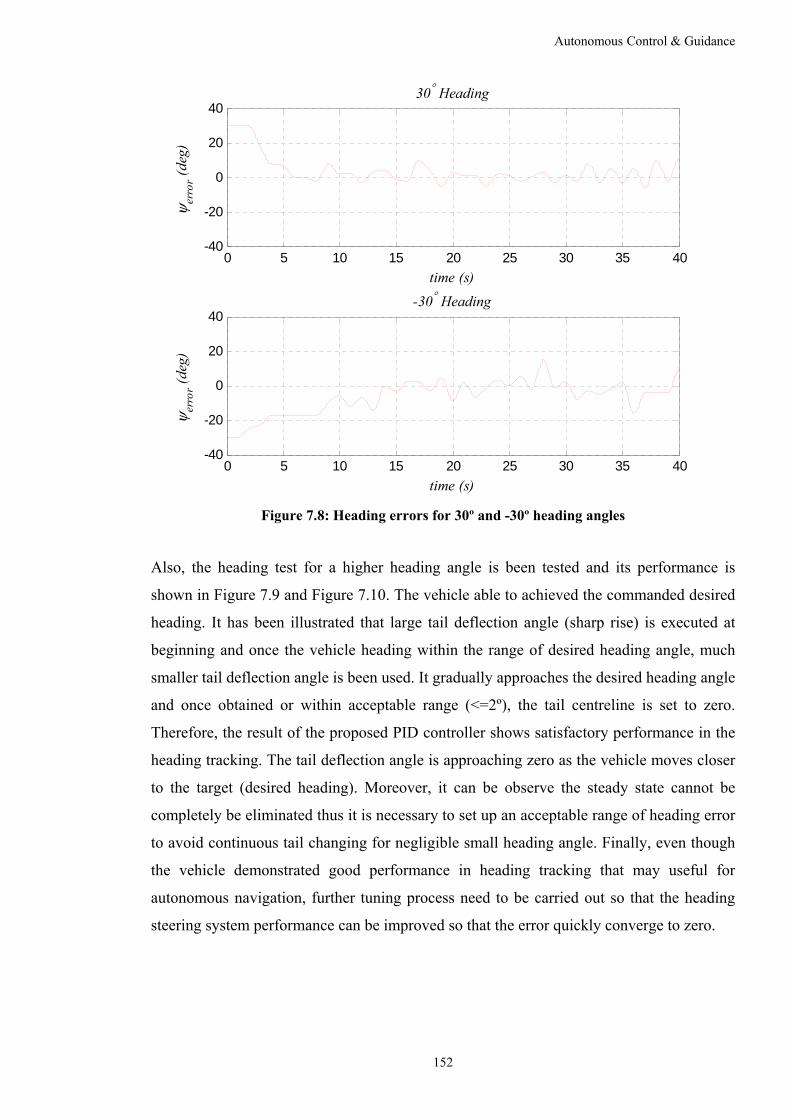
Autonomous Control & Guidance
152
Figure 7.8: Heading errors for 30º and -30º heading angles
Also, the heading test for a higher heading angle is been tested and its performance is
shown in Figure 7.9 and Figure 7.10. The vehicle able to achieved the commanded desired
heading. It has been illustrated that large tail deflection angle (sharp rise) is executed at
beginning and once the vehicle heading within the range of desired heading angle, much
smaller tail deflection angle is been used. It gradually approaches the desired heading angle
and once obtained or within acceptable range (<=2º), the tail centreline is set to zero.
Therefore, the result of the proposed PID controller shows satisfactory performance in the
heading tracking. The tail deflection angle is approaching zero as the vehicle moves closer
to the target (desired heading). Moreover, it can be observe the steady state cannot be
completely be eliminated thus it is necessary to set up an acceptable range of heading error
to avoid continuous tail changing for negligible small heading angle. Finally, even though
the vehicle demonstrated good performance in heading tracking that may useful for
autonomous navigation, further tuning process need to be carried out so that the heading
steering system performance can be improved so that the error quickly converge to zero.
0 5 10 15 20 25 30 35 40-40
-20
0
20
40
time (s)
er
ror (
deg)
30 Heading
0 5 10 15 20 25 30 35 40-40
-20
0
20
40
time (s)
er
ror (
deg)
-30 Heading

Autonomous Control & Guidance
153
Figure 7.9: The Vehicle performance in terms of heading and tail deflection angle with
desired heading of -60º (Experiment)
Figure 7.10: Heading errors for -60º heading angles
PID Simulation Results 7.5.1.2
The PID heading control system performance is illustrated in Figure 7.11 where the vehicle
is commanded to execute several heading course change. The vehicle is required to steer
into 60º, 0º, -60º and 0º heading. It can be seen the satisfactory of vehicle heading
controller performance where it able to track heading throughout the course changing. It
0 5 10 15 20 25 30 35 40 45-60
-40
-20
0
time (s)
T (
deg)
0 5 10 15 20 25 30 35 40 45
-60
-40
-20
0
time (s)
(
deg)
desired
0 5 10 15 20 25 30 35 40 45-60
-40
-20
0
20
40
time (s)
er
ror (
deg)

Autonomous Control & Guidance
154
can be noticed that the low values in tail deflection angle affected by the by the low
heading tracking error. The tracking errors converge to zero and the tail centreline revert to
its initial position for straight swimming as the desired heading is attained. Moreover, it
also demonstrated the symmetrical in controlled manoeuvre when the vehicle is directing
from 60º to 0º and -60º to 0º.
Figure 7.11: Vehicle heading motion based on change in tail centreline for PID controller.
The vehicle is commanded to 60º, 0º and 60º headings
Comparing the results of PID heading control performance for -60º heading angle between
experiment and simulation, it can be clearly seen the difference in the requirement of the
tail centreline need to achieved the desired heading. This is because the second order
reference model has been implemented in the simulation environment meanwhile in the
actual environment, it acts as a linear reference model which result a large tracking error.
As consequence, a sharp rise instead of gradually increases in tail deflection angle is
demanded by the system.
Sliding Mode Heading Controller 7.6
The sliding mode (McGookin, et al., 2000b; Fossen, 2011) is designed as an alternative
heading control system for the RoboSalmon. According to Utkin (2008) and Fossen (2011),
0 20 40 60 80 100 120-80
-40
0
40
80
time (s)
(
deg)
desired T
0 20 40 60 80 100 120-20
-10
0
10
20
time (s)
er
ror (
deg)

Autonomous Control & Guidance
155
the sliding mode can be considered as a robust nonlinear technique that is suitable for a
model that is operating under uncertainty conditions. It is found that the sliding mode
technique does not required the exact modelling (i.e. complex) since it is insensitive to the
unmodelled dynamics and external disturbance (McGookin, et al., 2000b; Utkin, 2008).
Healey & Lienard (1993) and McGookin, et al. (2000a) studies highlighted the advantages
of this technique to marine craft applications.
In this study, the controller purpose is to control the vehicle heading by providing the
required tail deflection angle, δT to the RoboSalmon model. Generally, the controller is
designed to make the state of the system follow some desired state response where the
difference (i.e. state error) can be quantified using Equation (7.4)
dx x x (7.4)
A single input, multistate (SIMS) (Healey & Lienard, 1993) system is designed for this
controller. The proposed sliding mode controller is realized by the decoupled three states
which are sway linear velocity, yaw angular velocity and yaw angular position from
equation of motion into the following single input state space equation.
h h h h Tx A x b (7.5)
Where xh is the state vector Ah, is the corresponding system matrix, bh is the input matrix and
δT is the tail deflection angle. This linearization of the vehicle equation is obtained through
small reference input. The δT is the control signal that will be provide to model where in
sliding mode control, the δT will consists of two components which are the nominal
equivalent control, δT_eq and the switching term δT_sw.
T T _eq T _sw (7.6)
These two component serve for the different purpose where the equivalent control used to
kept system states on the sliding mode meanwhile the switching control is used to drive the
system state reaching the sliding surface (Liu & Wang, 2011). The equivalent control (i.e.
linear controller) is designed about an equilibrium point for the system where it is chosen
as a state feedback gain controller (Healey & Lienard, 1993; McGookin, 1997; Fossen,

Autonomous Control & Guidance
156
2011) as shown in Equation (7.7) with k is the feedback gain obtained from pole placement
theory.
TT _ eq h hk x (7.7)
It is found that there is limitation on the effective operating condition of the controller,
outcome from the designed around a nominal linear plant (McGookin, et al., 2000b;
McGookin, et al., 2000a). Thus, a nonlinear switching term derived from a state hyperplane
(i.e. sliding surface, σh) has been introduced to compensate for variation in the vehicle
operating condition (McGookin, 1997). The sliding surface equation can be expressed as
follow:
Th h h h hdx h x x (7.8)
Differentiating with time
Th h h h hdx h x x (7.9)
Substituting Equations (7.5) ,(7.6) and (7.7) into Equation (7.9)
Th h h h h h T _ eq T _ sw hd
T Th h h h h h h T _ sw hd
T Th h h h h h h T _ sw hd
T Th h h h h h T _ sw hd
Th ch h h T _ sw hd
x h A x b x
h A x b k x b x
h A x b k x b x
h A b k x b x
h A x b x
(7.10)
It is simplified with a closed loop system matrix created by feedback gain, Ach.
Tch h h hA A b k (7.11)

Autonomous Control & Guidance
157
Rearranging Equation (7.10) with 0Th chh A
1
Th h h ch h h T _ sw hd
T T Th h h ch h h h T _ sw h hd
T T Th h T _ sw h ch h h hd h h
TT _ sw h chT
h h
x h A x b x
x h A x h b h x
h b h A x h x x
h Ah b
1
Th h hd h h
TT _ sw h hd h hT
h h
x h x x
h x xh b
(7.12)
Moreover, the term h (Healey & Lienard, 1993; Fossen, 2011) is given by
h h h h hx sgn x (7.13)
Therefore, the nonlinear control law be represent as
1 TT _ sw h hd h h hT
h h
h x sgn xh b
(7.14)
The switching gain ηh is used to determine the magnitude of this switching action while the
sgn (signum) function (McGookin, et al., 2000b; Fossen, 2011) provide the switching
action where it is used to indicate the direction of the sliding surface to the controller so
that Δxh can be drive to zero.
1 if 0
0 if 0
1 if 0
h
h h h
h
x
(7.15)
Healey & Lienard (1993) and Fossen (1994, 2011) found that the sgn can lead to chattering
where this effect needs to be eliminate for the controller to work properly. However, it is
found that it is better to replace the sgn by a continuous function tanh (the hyperbolic
tangent function) (Healey & Lienard, 1993; Akcakaya, et al., 2009; Fossen, 2011) where
the switching gain, ηh and boundary layer thickness, ϕh is selected to eliminate control
chattering (oscillation phenomenon).

Autonomous Control & Guidance
158
1 h hTT _ sw h hd hT
hh h
xh x tanh
h b
(7.16)
The total controller equation becomes
1 h hT TT h h h hd hT
hh h
xk x h x tanh
h b
(7.17)
The proposed sliding mode controller is realized by linearizing the equations system. As
been mentioned previously, the linearized equations will consist of three states which are
sway linear velocity, yaw angular velocity and yaw angular position. This linearization of
the vehicle equations are obtained through small reference input and can be rearranged into
single input space form equation as in Equation (7.5).
t d u
v
t d u v
z r
Y Y X ur murv
m Y
N N X uv Y uvr
I N
r
(7.18)
Table 7.1 listed the heading parameters that consist of closed loop poles, switching gain
and boundary layer that been chosen to determine the performance of sliding mode
heading controller. The poles represent the three states (i.e. v ,r , ) where two of the poles
need to be select while the third one is set zero (McGookin, et al., 2000a; Fossen, 2011).
The require feedback gain, k is obtained from pole placement theory. Then, h can be
measured as it is the right eigenvector of Ac (see Equation (7.5)) (McGookin, et al., 2000a;
Fossen, 2011). For the Matlab computation, referred to Fossen (2011)
Table 7.1: Sliding Mode heading controller parameters
Heading parameters
Closed loop poles, ph [ -0.31, -0.32, 0 ]
Switching gain, ηh 1.8
Boundary layer, ϕh 0.2

Autonomous Control & Guidance
159
The heading control law for tail centreline become
0 3238 0 0759 1 2796 0 3145T t . v t . r t . tanh . t (7.19)
It can be observed that the nonlinear switching term will consist only heading error, Δψ
while Δv(t) and Δr(t) are set to zero. This is due to the aim in this study that is to control
only the vehicle heading. The linear feedback of v(t) and r(t) terms are included for the
purpose to stabilize the sway or yaw dynamics (Healey & Lienard, 1993).
Sliding Mode Heading Controller Performance 7.6.1
The RoboSalmon is tested for heading tracking where the vehicle is commanded to steer
into 60º, 0º, -60º and 0º heading as previously done by the PID controller. Comparing
Figure 7.11 and Figure 7.12, similar vehicle responses have been observed for the sliding
mode heading controller where it is able to achieve the desired heading with reasonable
accuracy and the symmetrical vehicle response when operates on both heading direction.
The heading errors converge to zero as the vehicle approaching the desired heading. It also
has been noticed that the heading errors are corrected more quickly for the sliding mode
than the PID controller. Moreover, the tail deflection angle required for the sliding mode is
lower than the PID controller in order to acquire the same desired heading. Thus, it
suggests that the Sliding Mode controller perform better and efficiently than the PID for
the heading tracking manoeuvre.

Autonomous Control & Guidance
160
Figure 7.12: Vehicle heading motion based on change in tail centreline for sliding mode
controller. The vehicle is commanded to 60º, 0º and 60º headings
Line of Sight (LOS) 7.7
One of the objectives in this study is to design an autonomous biomimetic underwater
vehicle. In order to achieve this it is essential to have an efficient guidance system to guide
the vehicle along a predetermined path. Several guidance regimes that been applied to
AUVs have been reviewed by Naeem, et al. (2003) such as waypoint guidance using line
of sight (LOS) principles, vision-based guidance, Lyapunov based guidance and guidance
using chemical signals (e.g. sense chemical signal to locate the source of a chemical
discharge (Consi, et al., 1994)), proportional navigation guidance and electro-magnetic
guidance. It is found that the LOS guidance system is a popular choice for AUVs due to its
simple and effective implementation (Healey & Lienard, 1993; McGookin, et al., 2000a;
Fossen, et al., 2003).
0 20 40 60 80 100 120-80
-40
0
40
80
time (s)
(
deg)
desired T
0 20 40 60 80 100 120-40
-20
0
20
40
time (s)
er
ror (
deg)

Autonomous Control & Guidance
161
Figure 7.13. Autonomous guidance and heading control system
The LOS guidance system provides a heading command for the controller to follow, which
in turn provides the centreline steering signal for the vehicle to follow. The figure above
shows that the LOS guidance system is applied in series with the PID control system for
navigation along the predetermined course which is set out prior to autopilot activation
(McGookin, 1997). This course is made up of points known as waypoints. The vehicle is
guided from one waypoint to another by calculating the reference heading angle between
the vehicle current position and the waypoint position (Healey & Lienard, 1993; Fossen,
1994, 2011; Mazlan & McGookin, 2012) as shown in Figure 7.14 where Equation (7.20) is
used to measure the heading angle, ψref .
Figure 7.14: Waypoint and acceptance radius
1 where wp pref ref
wp p
y ytan
x x
(7.20)

Autonomous Control & Guidance
162
It is noted that the ψref range lies between –π and π where there is a discontinuity at the
-π/π. This could create a calculating error when measuring ψref such as changing from
negative to positive or positive to negative heading. This rapid change can be prevent by
introducing reference heading so that ψref can be varies from –∞ to +∞ (Breivik, 2003;
Fossen, et al., 2003). This heading angle, ψref is then compared to the current vehicle
heading, ψ and serves as input for the steering controller. The controller used the difference
to compute the required tail centreline deflection. The tail centreline signal steers the
vehicle towards the specific target waypoint until it comes within range of the waypoint
coordinates (xwp, ywp). This range, Rk, is called the radius of acceptance and it forms a circle
of acceptance around the waypoint. Equation (7.21) shows the expression used to calculate
the acquisition of a waypoint (Fossen, et al., 2003).
2 2 2wp p wp p kx x y y R (7.21)
The (xwp , ywp) is waypoint stored in waypoint table, (xp , yp) is the current position of the
vehicle and the radius for the circle of acceptance, Rk is defined as n times of vehicle
length where typically, it is selected between one and three vehicle lengths (McGookin, et
al., 2000b). In this study, the radius for the circle of acceptance is chosen to be equal to one
vehicle length. Once the vehicle’s position is within the circle of acceptance of the current
waypoint, the next waypoint in the list is acquired and the vehicle starts to navigate
towards it.
Table 7.2: Waypoints
Waypoint No. Coordinate (x, y)
1 ( 3 , 3)
2 (-3 , 3)
3 ( 3 , -3)
4 (-3 , -3)
The PID controller applied in series with the LOS guidance system has been carried out in
simulation where the vehicle is instructed to navigate through 4 waypoints in a 2D plane
are listed in Table 7.2 with the radius of acceptance for all waypoints is set to one vehicle
length (i.e. 0.90 m). These waypoints have been arranged in that manner so that the vehicle

Autonomous Control & Guidance
163
path trajectory will resemble ‘∞’ shape while the distance between each waypoint is set
approximately 6 m which appropriate to the RoboSalmon turning ability (i.e. over half of
its body length) that has been analysed in Chapter 6.
The vehicle trajectory is shown in Figure 7.15 where it shows good performance of the
PID heading controller and LOS guidance system. The controller has successfully
demonstrated that it can guide the vehicle from one waypoint to another based on the LOS
heading measurement. Once the vehicle within the circle of acceptance of the current
desired waypoint, it updates to the next desired waypoint. This process is repeated until all
waypoints are achieved. It took less than 300 seconds for vehicle to complete the
navigation throughout the waypoints with the average surge velocity is measured at 0.0846
m/s.
Figure 7.15: Line of sight guidance system for waypoint tracking with PID controller
-6 -5 -4 -3 -2 -1 0 1 2 3 4 5 6-5
-4
-3
-2
-1
0
1
2
3
4
5
y (m)
x (m
)
waypoint 3 waypoint 1
waypoint 2waypoint 4

Autonomous Control & Guidance
164
Figure 7.16: PID controller performance on vehicle tracking angle and tail centreline
Figure 7.17 illustrates the relationship between the change in tail centreline and motor (i.e.
tail undulation) current. It can be seen that the change in tail centreline will results higher
current demand by the motor in order to produce the require tail deflection angle. As
consequence, it contributes to higher power consumption with an average power consumed
by the vehicle is measured at 7.58 W.
0 50 100 150 200 250 300-200
0
200
400
time (s)
(
deg)
desired T
0 50 100 150 200 250 300-100
-50
0
50
100
time (s)
er
ror (
deg)

Autonomous Control & Guidance
165
Figure 7.17: PID controller performance on the tail centreline relates to motor current
Next, the sliding mode controller was tested is series with the LOS guidance system and
Figure 7.18 shows the vehicle path trajectory throughout the 4 waypoints. It has
demonstrated that the sliding mode perform well with the LOS guidance. A similar
analysis of PID controller performance can be made to the sliding mode controller such as
the heading tracking error converges to zero as the vehicle approaches the waypoint (see
Figure 7.19) and high current is consumed when altering the tail centreline (see Figure
7.20). The vehicle implemented with sliding mode controller has an average surge velocity
of 0.0867 m/s and average power consumption of 7.57 W.
0 50 100 150 200 250 300-50
-25
0
25
50
time (s)
T
0 50 100 150 200 250 300-2
-1
0
1
time (s)
Cur
rent
(A
)

Autonomous Control & Guidance
166
Figure 7.18: Line of sight guidance system for waypoint tracking with sliding mode controller
Figure 7.19: Sliding mode controller performance on vehicle tracking angle and tail
centreline
-6 -5 -4 -3 -2 -1 0 1 2 3 4 5 6-5
-4
-3
-2
-1
0
1
2
3
4
5
y (m)
x (m
)
Waypoint 3 Waypoint 1
Waypoint 4 Waypoint 2
0 50 100 150 200 250 300-200
0
200
400
time (s)
(
deg)
desired T
0 50 100 150 200 250 300-100
-50
0
50
100
time (s)
er
ror (
deg)

Autonomous Control & Guidance
167
The performance of these controllers are been compared and analysed, it can be observed
the path trajectory generate by this two controllers are different (see Figure 7.15 and Figure
7.18). This is due to the difference alteration angle of vehicle tail centreline. The amplitude
of tail deflection angle measured by the PID controller is higher than sliding mode
controller (see Figure 7.16 and Figure 7.19). Therefore, the bigger tail deflection angle
requires the vehicle to bend its body which then produce higher turning angle (i.e. sharp
turning). This action decreases the vehicle surge velocity as most of generated thrust turn
into sway velocity. Furthermore, much higher current and power is consumed to execute
bigger tail deflection angle. Therefore, it can be conclude that the sliding mode perform
slightly better than PID controller since it can efficiently guide the vehicle to manoeuvre
throughout the waypoints without forcing bigger tail deflection angle and high current
consumed.
Figure 7.20: Sliding mode controller performance on the tail centreline relates to motor
current
Summary 7.8
This chapter highlights a RoboSalmon navigation system that consists of a heading control
system and a guidance system. Two sets of heading controller have been designed based
on PID and sliding mode control theory. The heading controller has been implemented on
0 50 100 150 200 250 300-40
-20
0
20
40
time (s)
T
0 50 100 150 200 250 300-1.5
-1
-0.5
0
0.5
1
time (s)
Cur
rent
(A
)

Autonomous Control & Guidance
168
the RoboSalmon to track the vehicle heading where the heading can be adjusted by
manipulating the tail centreline. Both controller performances have been analysed and it
can observed that both able to guide the vehicle to achieve the desired heading with
reasonable accuracy with the heading errors converge to zero. Furthermore, it also can be
seen that the symmetrical vehicle response when operates on both heading direction. From
the results obtained, the sliding mode heading controller performed better and efficiently
than the PID for the heading tracking manoeuvre since the heading errors are corrected
more quickly. Moreover, the requirement of altering tail deflection angle is lower for the
sliding mode than the PID controller in order to gain the same vehicle desired heading.
Finally, a line of sight has been implemented where it used to guide the RoboSalmon
through certain path made from several waypoints.

Discussion, Conclusions & Further Work
169
8
Discussion, Conclusions
& Further Work
Discussion and Conclusions 8.1
The modelling, simulation, control and construction of a biomimetic underwater vehicle
known as RoboSalmon have been presented in this thesis. The design of this vehicle is
based on the physiology of an adult Atlantic salmon where approximately half of its body
(i.e. the tail) performs an undulation motion in order to propel it forward. It has been
designed with a multiple jointed fully actuated tail that is used to replicate the undulation
tail gait of a real fish. The complexity of the design has been described in detailed in
Chapter 3 which also includes the component configurations that are involved in the
motion control of the multiple actuator motors, the motion detection by sensors, power
system and data collection.
Chapter 4 discusses the development of a multi-variable mathematical model that describes
the dynamics and electro-mechanics of this biomimetic underwater vehicle. This
mathematical model is used to estimate the kinematic relationships for the tail, the
vehicle’s static hull and its head. In addition, the model contains expressions describing the
rigid body dynamics and associated hydrodynamics of the vehicle. These aspects are
modelled using conventional marine vessel techniques with several modifications made to
incorporate the thrust production from the tail. In the model this is achieved by considering
the undulatory motion of real fish tail as a travelling wave. Thus a simple gait has been
developed to represent this undulation motion and the model of the tail itself is based on a
multi-jointed robotic manipulator arm. The fusion of these modelled elements provides a
very complex model that accurately represents the swimming performance for this
biomimetic underwater vehicle.

Discussion, Conclusions & Further Work
170
In Chapter 5 experiments concerning the vehicle’s forward swimming are presented.
These involve the analysis of varying several tail beat parameters, amplitude and
frequency. The results obtained showed the linear increase in the surge velocity related to
these parameters. Even though actuator saturation occurred, it was observed the effect of
increasing the tail beat frequency and keeping the amplitude constant at a value of 0.05 m
where the vehicle’s surge velocity is increasing. Similar observations have been made
when varying the tail beat amplitude while maintaining a constant frequency. The highest
surge velocity measured during these experiments was 0.143 ms-1 when the tail beat
frequency and amplitude are set at 1 Hz and 0.15 m respectively.
Numbers of computer simulation studies have been carried out based on the mathematical
model developed in Chapter 4. These computer simulations have been a powerful tool for
predicting the vehicle performance when actuator saturation and other physical limitations
prevented true experimental analysis to be performed. The result obtained from simulation
model agreed with the experimental observation where the vehicle surge velocity increases
based on the increase in tail beat amplitude and frequency. However, the ranges of forward
speeds achieved by the physical vehicle are much lower than the estimated values for real
salmon. This disparity is due to the mechanical limitations imposed by the tail actuators.
Thus, an improvement in the operational specification of the motors used to actuate the tail
sections would provide an increased range of achievable velocities. The required motor
speed specification is suggested to be at least 160 rpm to meet the design of tail beat
amplitude (i.e. 0.05 - 0.20 m) and frequency (i.e. 0.5 - 3.0 Hz).
In addition to swimming performance, the vehicle propulsion efficiency has been
investigated and analysed. It has been found that the efficiency increased linearly with
swimming speed up to a maximum measured efficiency value of 2.14%. Moreover, it is
suggested that the efficiency improved when vehicle is operate at higher and larger tail
beat frequency and amplitude. The reason for low efficiency values is due to the recoil
motion experienced by the vehicle. This adverse motion is the reaction force from the tail
which causes the vehicle to roll and pitch during each undulation cycle. The utilisation of
an actuated head during forward swimming to counteract the recoil of the has been tested
but the results indicated that it produces an even larger recoil motion, which in turn
contributed to the decrease in the magnitude of the vehicle’s surge velocity.
The manoeuvring experimentation and simulation studies were next analysed where the
vehicle has been tested with cruise in turning and zig-zag swimming patterns. This

Discussion, Conclusions & Further Work
171
involved varying the same tail parameters used for forward swimming (i.e. tail beat
frequency f and tail beat amplitude A) with the addition of tail deflection angle, δT. This
tail deflection angle is used to change the vehicle heading. The cruise in turn manoeuvring
pattern is designed where the vehicle tail centreline is deflected to a predefined angle and
holding it constant until circular path is obtained. Several sets of tail beat configurations
have been tested with different values of tail deflection angle. Here, one of characteristics
been measured is the vehicle turning radius. It has been observed that when the tail beat
amplitude and frequency are keep constant, increases in tail deflection angle produces
increase in vehicle roll and yaw angular velocities which in turn results in a decrease in the
vehicle turning radius. The similar pattern has been observed when the tail beat frequency
is set to increase but when the vehicle turning radius vehicle act oppositely when it is
applied with larger tail beat amplitude. During manoeuvring, it can be noticed that the
vehicle surge velocity decreases compared to surge velocity for forward motion. This is
expected since some of the thrust propulsion is used to generate the turning motion and
becomes sway velocity.
The smallest turning radius that the vehicle able to attain is 0.58 m which is just over half
of its body length when operated at the largest tail deflection angle. This also demonstrated
it has smaller turning radius than the conventional underwater vehicles that in general tend
to have an average turn radius of 3 -15 times of the body length. The vehicle experimental
manoeuvring performance also has been compared to the results obtained using computer
simulation. It has been found that the simulation model is reasonably accurate to represent
the actual system. Thus, it proves useful where this model can be used to estimate the
vehicle performance for the tail deflection angles that have not been tested experimentally.
The RoboSalmon has been simulated to turn in both directions (i.e. left/right) for varies tail
deflection angles. The vehicle shows a symmetrical path trajectory and smaller tuning
radius able to be produced when larger tail deflection angle been applied. The zig-zag
manoeuvre is another pattern that been simulated to evaluate the vehicle manoeuvring
capability. The vehicle tail deflection angle is commanded to be 20º from an initially
straight course and this heading is maintained until the vehicle heading reached the desired
heading. Then the tail centreline is deflected to the opposite direction. The vehicle exhibits
a high manoeuvrability performance with the time to change its heading from the time tail
centre being execute depends on the tail beat parameters. It was found that the time
duration to complete one cycle is shorter when operated at larger tail beat amplitude and
higher frequency.

Discussion, Conclusions & Further Work
172
Finally, RoboSalmon heading and guidance control system have been discussed in order to
enable it to navigate without human intervention. Two types of heading controller have
been designed based on PID and sliding mode control theory. These heading controllers
were used to track the vehicle heading where the heading can be adjusted by altering the
tail centreline. The results obtained from both controllers show satisfactory performance in
the heading tracking. Both controllers were able to guide the vehicle to achieve the desired
heading with reasonable accuracy and shown that the heading errors converge to zero.
Moreover, it was suggested that the sliding mode heading controller performed better and
efficiently than the PID heading the controller for the heading tracking manoeuvre. It can
be observed that the heading error in sliding mode controller is corrected more quickly
than in the PID controller. Furthermore, it required lower tail deflection angle to achieve
the same vehicle desired heading.
A line of sight guidance system was introduced where it used to guide the RoboSalmon
through certain path made by several waypoints. The vehicle will move from one waypoint
to another once it reaches within the radius of acceptance acceptable that is situated around
the waypoint. The results show that the vehicle capable to navigate through set of
waypoints to form ‘∞’ shape. It took less than 300 seconds simulation time for the vehicle
to complete the shape. The PID controller measured an average surge velocity of 0.0846
m/s and average power consumption of 7.58 W while the sliding mode controller has an
average surge velocity of 0.0867 m/s and average power consumption of 7.57 W.
In conclusion, the design work and control of an autonomous underwater vehicle that
mimics a fish tail propulsion system has been investigated in this research. The work was
to determine whether this system can be considered as an alternative option to the current
AUV design. The approach of using multiple jointed fully actuated tail allows the
replication of the undulation swimming gait of the real fish. The vehicle has exhibits
experimentally that it capable to swim and perform basic manoeuvres. This work also
involved developing a mathematical model which was used to validate the vehicle
performance. The simulation data show that it reasonably agreed with the data obtainable
from experimentation. Thus, it proved to be useful tool as it can also be used to predict the
vehicle performance for several manoeuvres that been able to be tested experimentally that
includes the autonomous navigation through waypoints. Another conclusion can be made
is that the sinusoidal shape of undulation movement helps to reduce vehicle recoil motion
when compared to the tendon drive system in Watts (2009) research. As consequences, this
should contribute to a higher vehicle surge velocity. However due to under specified

Discussion, Conclusions & Further Work
173
actuator selection, the vehicle surge velocity cannot be tested for a higher and larger tail
beat frequency and amplitude respectively. Even at low speed, the vehicle tends to have a
higher propulsion efficiency compared to propeller based model when operate at the same
condition. According to the results obtained from the simulation model, there is potential
for the vehicle’s swimming speeds to be improved if the actuators are better specified.
This vehicle also demonstrates a higher manoeuvrability corresponding to the flexibility in
multilink tail manipulation and the vehicle able to perform 180º turn with less than one
body length. This proposes that the RoboSalmon has superior turning ability than
conventional underwater vehicles. Although the experimental stage of this study
encountered actuator limitation, it can be deduced that the RoboSalmon forward and
manoeuvring capability may have advantages over the conventional AUVs. Thus, it
suggests that the biomimetic fish tail system can be considered as a suitable alternative to
the current AUVs propulsion system that generally based on propeller.
Further Work 8.2
It is very apparent that the design and construction of this biomimetic underwater vehicle
incorporates multi-disciplinary subject areas such as naval, mechanical, computer,
electrical and electronics engineering. Many lessons have been learned throughout this
study and the work presented has the potential to be expanded further in order to improve
the vehicle performance. Some ideas for further work to expand the scope of this research
are outlined in the sections below.
Modelling and Simulation 8.2.1
The mathematical model has been validated in this research and it can be observed that it
sufficiently represent the actual vehicle performance. Thus in the future, a control law can
be introduced for vehicle speed and diving control. This includes diving and climbing
manoeuvres where a 3D simulation can be generated. This computer simulation can also be
extended in order to produce more realistic conditions. These include the presence of
disturbance in physical environment such as ocean current and sensor noise. In addition,
the vehicle navigation performance can be improved by implementing an obstacle
avoidance algorithm into the simulation.

Discussion, Conclusions & Further Work
174
RoboSalmon System Improvement 8.2.2
As been mentioned in Chapter 3, a latex skin has been developed to contain the electronic
components and one of the problems encountered during experimentation concern
waterproofing the tail undulation part. There are cases that water flooding the undulation
part due to improper seal and the degrading of latex skin condition over time. Even though
the circuit board is well protected, the water still can cause damage to the actuator part and
disturb the vehicle buoyancy force where the vehicle starts to sink. Thus, in order to
prevent future electrical problem, individual actuator housing can be implemented in
addition to provide extra precaution when reapplying seal toward the latex skin.
The design of printed circuit board (PCB) also can be improved where currently, all PCB
are designed only for double sided layers. If a multilayer option is available, it can be a
useful addition especially for the tail part controller since it will take less space and reduce
wiring connections. This will also help to reduce the complexity in case of system
troubleshooting and allow for additional sensors to be placed.
The mathematical model of vehicle with the fish like propulsion system has been designed
in 6 degree of freedom, though only 5 parameters are available to be validated which are
surge, sway, roll, pitch and yaw. Unfortunately, heave dynamics cannot be validated since
the current prototype does not have the capability of changing its operational depth. A pair
of pectoral fins is designed and mounted on each side of the body in order to allow vehicle
depth control. However, the offset in pectoral fin alone not sufficient to cause the vehicle
to dive. An alternative method needs to be introduced and it is known that fish are able to
dive up and down as part of their routine of feeding and avoiding predators by changing
the volume of the swim bladder (Bone, et al., 1995). Thus, a similar concept can be used
for the underwater vehicle by employing artificial bladder or ballast tank. The vehicle
vertical movement can then be control by alternately filled with water or air where filling it
with air in order to float or water in order to submerge. Other further possible areas that
can be expanded from this research include multiple vehicle coordination, implementing
other types of control and guidance methodologies for autonomous swimming and
integration of sensors for the purpose of obstacle avoidance.

175
References Afolayan, M. O., Yawas, D. S., Folayan, C. O., & Aku, S. Y. (2012). Mechanical
Description of a Hyper-Redundant Robot Joint Mechanism Used for a Design of a
Biomimetic Robotic Fish. Journal of Robotics, 2012, 16.
Akcakaya, H., Yildiz, H. A., Saglam, G., & Gurleyen, F. (2009). Sliding Mode Control of
Autonomous Underwater Vehicle. Proceedings of the International Conference on
Electrical and Electronics Engineering, ELECO 2009, Bursa, Turkey, 332-336.
Allegro MicroSystems. (n.d.). Fully Integrated, Hall Effect-Based Linear Current Sensor
IC with 2.1kVRMS Isolation and a Low-Resistance Current Conductor (pp. 15).
Allen, B., Vorus, W. S., & Prestero, T. (2000). Propulsion System Performance
Enhancements on REMUS AUVs. Proceedings of the MTS/IEEE Conference and
Exhibition, OCEANS 2000 Rhode Island, 1869-1873.
American Bureau of Shipping. (2006). Guide for Vessel Maneuverability (pp. 124).
Houston, TX.
Analog Devices. (2013). ADXL345: 3-Axis, ±2 g/±4 g/±8 g/±16 g Digital Accelerometer
Data Sheet (pp. 40). Norwood, MA, USA.
Anderson, J. M., & Chhabra, N. K. (2002). Maneuvering and Stability Performance of a
Robotic Tuna. Integr. Comp. Biol., 42(1), 118-126.
Anderson, J. M., & Kerrebrock, P. A. (2002). Biomimetics in Action: Design and
Performance of an Autonomous Robotic Fish. In J. Ayers, J. L. Davis & A. Rudolph
(Eds.), Neurotechnology for Biomimetic Robots (pp. 297-308). London, England: MIT
Press.
Apalkov, A., Fernández, R., Fontaine, J. G., Akinfiev, T., & Armada, M. (2012).
Mechanical Actuator for Biomimetic Propulsion and the Effect of the Caudal Fin Elasticity
on the Swimming Performance. Sensors and Actuators A: Physical, 178(0), 164-174.

176
Araujo, J., Sandberg, H., & Johansson, K. H. (2009). Experimental Validation of a
Localization System Based on a Heterogeneous Sensor Network. Proceedings of the 7th
Asian Control Conference Hong Kong, China, 465-470.
Arnold, M. (2007). Multi-Rate Time Integration for Large Scale Multibody System
Models. In P. Eberhard (Ed.), Proceedings of the IUTAM Symposium on Multiscale
Problems in Multibody System Contacts (Vol. 1, pp. 1-10): Springer Netherlands.
Åström, K. J. (2002). PID Control. Control System Design (pp. 36).
Atlas Elektronik GmbH. (2013). Atlas SeaOtter. AUV for Multi-Purpose Underwater
Operations (pp. 1-4 ). Bremen, Germany.
Attaway, S. (2013). Sights and Sounds. In S. Attaway (Ed.), Matlab (3rd ed., pp. 419-460).
Boston: Butterworth-Heinemann.
Bainbridge, R. (1957). The Speed of Swimming of Fish as Related to the Size and to the
Frequency and Amplitude of Tail Beat. Journal of Experimental Biology, 35, 109-133.
Balci, O. (1994). Validation, Verification, and Testing Techniques Throughout the Life
Cycle of a Simulation Study. Proceedings of the Winter Simulation Conference,
Piscataway, New Jersey, 215-220.
Ballard, R. D. (1993). The JASON Remotely Operated Vehicle System: Woods Hole
Oceanographic Institution
Bandyopadhyay, P. R. (2004). Guest Editorial: Biology-Inspired Science and Technology
for Autonomous Underwater Vehicles. IEEE Journal of Oceanic Engineering, 29(3), 542-
546.
Bandyopadhyay, P. R. (2005). Trends in Biorobotic Autonomous Undersea Vehicles. IEEE
Journal of Oceanic Engineering, 30(1), 109-139.
Bar-Cohen, Y. (2006). Biomimetics - Using Nature to Inspire Human Innovation.
Bioinspiration & Biomimetics, 1, 12.
Barrett, D., Grosenbaugh, M., & Triantafyllou, M. (1996). The Optimal Control of a
Flexible Hull Robotic Undersea Vehicle Propelled by an Oscillating Foil. Proceedings of

177
the 1996 Symposium on Autonomous Underwater Vehicle Technology. AUV '96,
Monterey, CA, 1-9.
Barrett, D. (2002). Optimization of Swimming Locomotion by Genetic Algorithm. In J.
Ayers, J. L. Davis & A. Rudolph (Eds.), Neurotechnology for Biomimetic Robots (pp. 207-
221). London, England: MIT Press.
Barton, M. (2007). Bond's Biology of Fishes (3rd ed.). Belmont, CA: Thomas Brooks/Cole.
Bednar, R., & Crosbie, R. E. (2007). Stability of Multi-rate Simulation Algorithms. Paper
presented at the 2007 Summer Computer Simulation Conference, San Diego, California.
Beem, H. R., & Triantafyllou, M. (2012). Biomimetic Design of an Undulatory Stingray
AUV Fin. Proceedings of the International Society of Offshore and Polar Engineers
(ISOPE), Rhodes, Greece, 1 - 5.
Bellingham, J. (2001). Autonomous Underwater Vehicles (AUVs). Academic Press, 212-
216.
Bellingham, J. G., Goudey, C. A., Consi, T. R., Bales, J. W., Atwood, D. K., Leonard, J. J.,
& Chryssostomidis, C. (1994). A Second Generation Survey AUV. Proceedings of the 1994
Symposium on Autonomous Underwater Vehicle Technology, Cambridge, MA, 148-155.
Bende, V., Pathak, P. M., Dixit, K. S., & Harsha, S. (2012). Energy Optimal Trajectory
Planning of an Underwater Robot using a Genetic Algorithm. Proceedings of the
Institution of Mechanical Engineers, Part I: Journal of Systems and Control Engineering,
226(8), 1077-1087.
Bhandari, S. A., Rana, A. D., Bhandari, S. Z., Kalange, V. A., & Sanghvi, M. R. (2012).
Mathematical Model for Digital Video Watermarking based on 3D Wavelet Transform.
Proceedings of the International Conference in Computational Intelligence (ICCIA2012)
New York, USA.
Blake, R. W. (1983). Fish Locomotion. New York: Cambridge University Press.
Blake, R. W. (2004). Fish Functional Design and Swimming Performance. Journal of Fish
Biology, 65(5), 1193-1222.

178
Blidberg, D. R. (2001). The Development of Autonomous Underwater Vehicles (AUV); A
Brief Summary. Proceedings of the IEEE International Conference on Robotics and
Automation, Seoul, Korea.
Bluefin Robotics. (2014). Propulsion Retrieved Oct 7 2014, from
http://www.bluefinrobotics.com/technology/propulsion/
Bohn, C., & Atherton, D. P. (1995). An Analysis Package Comparing PID Anti Windup
Strategies. IEEE Control Systems, 15(2), 34-40.
Bolton, W. (2008). Mechatronics: Electronic Control systems in Mechanical and
Electrical Engineering (4th ed.). Essex, England: Prentice Hall.
Bone, Q., Marshall, N. B., & Blaxter, J. H. S. (1995). Biology of Fishes: Chapman & Hall.
Bowen, A. D., Yoerger, D. R., Taylor, C., McCabe, R., Howland, J., Gomez-Ibanez, D.,
Kinsey, J. C., Heintz, M., McDonald, G., Peters, D. B., Fletcher, B., Young, C., Buescher,
J., Whitcomb, L. L., Martin, S. C., Webster, S. E., & Jakuba, M. V. (2008). The Nereus
Hybrid Underwater Robotic Vehicle for Global Ocean Science Operations to 11,000 m
Depth. Proceedings of the OCEANS 2008, Quebec, 1-10.
Brege, E. D. (2011). Design and Construction of a Low Cost, Modular Autonomous
Underwater Vehicle. Naval Engineer and Master of Science in Mechanical Engineering,
Massachusetts Institute of Technology, USA.
Breivik, M. (2003). Nonlinear Maneuvering Control of Underactuated Ships. MSc,
Norwegian University of Science and Technology, Trondheim, Norway.
Brun, L. (2012). ROV/AUV Trends. Market and Technology. Marine Technology
Reporter, 55, 48 - 51.
Budiyono, A. (2009). Advances in Unmanned Underwater Vehicles Technologies:
Modeling, Control and Guidance Perspectives Indian Journal of Marine Sciences, 38(3),
282-295.
Cau, A., Concas, G., Melis, M., & Turnu, I. (2005). Evaluate XP Effectiveness Using
Simulation Modeling. In H. Baumeister, M. Marchesi & M. Holcombe (Eds.), Extreme
Programming and Agile Processes in Software Engineering (Vol. 3556, pp. 48-56):
Springer Berlin Heidelberg.

179
Cen, L., & Erturk, A. (2013). Bio-inspired Aquatic Robotics by Untethered
Piezohydroelastic Actuation. Bioinspiration & Biomimetics, 8(1), 13.
Chadwick, B. (2010). Remotely Operated Vehicles (ROVs) and Autonomous Underwater
Vehicles (AUVs) Retrieved 15th August, 2014, from
http://oceanexplorer.noaa.gov/explorations/02fire/background/rovs_auvs/rov_auv.html
Chapra, S. C., & Canale, R. P. (2003). Numerical Methods for Engineers with Software
and Programming Applications (4th ed.): McGraw-Hill.
Chen, Z., Shatara, S., & Tan, X. (2010). Modeling of Biomimetic Robotic Fish Propelled
by An Ionic Polymer–Metal Composite Caudal Fin. IEEE/ASME Transactions on
Mechatronics, 15(3), 448-459.
Chopra, M. G. (1976). Large Amplitude Lunate-tail Theory of Fish Locomotion. Journal
of Fluid Mechanics, 74(01), 161-182.
Christ, R. D., & Wernli Sr, R. L. (2014). The ROV Business. In R. D. Christ & R. L.
Wernli (Eds.), The ROV Manual (2nd ed., pp. 3-20). Oxford: Butterworth-Heinemann.
Chu, W.-S., Lee, K.-T., Song, S.-H., Han, M.-W., Lee, J.-Y., Kim, H.-S., Kim, M.-S.,
Park, Y.-J., Cho, K.-J., & Ahn, S.-H. (2012). Review of Biomimetic Underwater Robots
using Smart Actuators. International Journal of Precision Engineering and
Manufacturing, 13(7), 1281-1292.
Colgate, J. E., & Lynch, K. M. (2004). Mechanics and Control of Swimming: A Review.
IEEE Journal of Oceanic Engineering, 29(3), 660-673.
Conry, M., Keefe, A., Ober, W., Rufo, M., & Shane, D. (2013). BIOSwimmer: Enabling
Technology for Port Security. Proceedings of the IEEE International Conference on
Technologies for Homeland Security (HST), 2013, Waltham, Massachusetts, USA, 364-
368.
Conservation of Atlantic Salmon in Scotland Project. (2010). The Atlantic Salmon (Salmo
Salar L) Retrieved 1st May, 2011, from http://www.snh.org.uk/salmonlifeproject
Consi, T. R., Atema, J., Goudey, C. A., Cho, J., & Chryssostomidis, C. (1994). AUV
Guidance with Chemical Signals. Proceedings of the 1994 Symposium on Autonomous
Underwater Vehicle Technology, Piscataway, New Jersey, USA, 450-455.

180
Corfield, S., & Hillenbrand, C. (2002). Defence Applications for Unmanned Underwater
Vehicles. In G. Griffiths (Ed.), Technology and Applications of Autonomous Underwater
Vehicles (pp. 161-178): CRC Press.
Danson, E. F. S. (2002). AUV Tasks in the Offshore Industry. In G. Griffiths (Ed.),
Technology and Applications of Autonomous Underwater Vehicles (pp. 127-138): CRC
Press.
Dart, F. (2009). Interfacing a USB Flash Drive to a PIC Microcontroller. Retrieved from
http://www.newelectronics.co.uk/embedded-electronics-technology/interfacing-a-usb-
flash-drive-to-a-pic-microcontroller/17222/
Davies, J. H. (2011, 6th October). A Basic Introduction to Cadence OrCAD PCB Designer
Version 16.3 [unpublished lecture notes]. Glasgow University, 70.
DELTRON Enclosures. (n.d.). Aluminium Enclosure IP68 Plain, from http://www.dem-
uk.com/deltron-enclosures/products/ip68_enclosures/aluminium_enclosure_ip68_plain/
Domenici, P., & Blake, R. W. (1997). The Kinematics and Performance of Fish Fast-Start
Swimming. Journal of Experimental Biology, 200, 1165–1178.
Donley, J. M., Sepulveda, C. A., Konstantinidis, P., Gemballa, S., & Shadwick, R. E.
(2004). Convergent Evolution in Mechanical Design of Lamnid Sharks and Tunas.
[10.1038/nature02435]. Nature, 429(6987), 61-65.
Edwards, C., & Postlethwaite, I. (1999). An Anti-windup Scheme with Closed-loop
Stability Considerations. Automatica, 35(4), 761-765.
Ellerby, D. J. (2010). How Efficient is a Fish? Journal of Experimental Biology, 213(22),
3765-3767.
Eloy, C. (2012). Optimal Strouhal Number for Swimming Animals. Journal of Fluids and
Structures, 30(0), 205-218.
Elvander, J., & Hawkes, G. (2012). ROVs and AUVs in Support of Marine Renewable
Technologies. Proceedings of the Oceans 2012, Hampton Roads, Virginia, 1-6.
Eng You, H., Hong Geok, S., & Chitre, M. (2010). Depth Control of an Autonomous
Underwater Vehicle, STARFISH. Proceedings of the IEEE OCEANS 2010, Sydney, 1-6.

181
Engelhardtsen, Ø. (2007). 3D AUV Collision Avoidance. MSc, Norwegian University of
Science and Technology, Trondheim, Norway. Retrieved from
http://urn.kb.se/resolve?urn=urn:nbn:no:ntnu:diva-9534
Eskesen, J., Owens, D., Soroka, M., Morash, J., Hover, F. S., & Chrysosstomidis, C.
(2009). Design and Performance of ODYSSEY IV: A Deep Ocean Hover-Capable AUV
(pp. 10). Cambridge, Massachusetts: MIT Sea Grant College Program.
Faltinsen, O. M. (2006). Maneuvering Hydrodynamics of High-Speed Marine Vehicles (pp.
390-434): Cambridge University Press.
Fiazza, C., Salumae, T., Listak, M., Kulikovskis, G., Templeton, R., Akanyeti, O., Megill,
W., Fiorini, P., & Kruusmaa, M. (2010). Biomimetic Mechanical Design for Soft-Bodied
Underwater Vehicles. Proceedings of the OCEANS 2010 IEEE, Sydney, 1-7.
Finnish Game and Fisheries Research Institute. (2008). Atlantic salmon (Salmo salar),
from http://www.rktl.fi/english/fish/fish_atlas/atlantic_salmon/
Fish, F. E. (1997). Biological Designs for Enhanced Maneuverability: Analysis of Marine
Mammal Performance. Proceedings of the 10th International Symposium on Unmanned
Untethered Submersible Technology, Special Session on Bio-Engineering Research
Related to Autonomous Underwater Vehicles, Durham, NH, 109 -117.
Fossen, T. I. (1994). Guidance and Control of Ocean Vehicles: John Wiley & Son, Ltd.
Fossen, T. I., Breivik, M., & Skjetne, R. (2003). Line-Of-Sight Path Following Of
Underactuated Marine Craft. Proceedings of the 6th IFAC MCMC, Girona, Spain, 244-
249.
Fossen, T. I., & Johansen, T. A. (2006). A Survey of Control Allocation Methods for Ships
and Underwater Vehicles. Proceedings of the 14th Mediterranean Conference on Control
and Automation, MED '06, Ancona, Italy, 1-6.
Fossen, T. I. (2011). Handbook of Marine Craft Hydrodynamics and Motion Control: John
Wiley & Son, Ltd.
Fountain, H. (2010). ABE, Pioneering Robotic Undersea Explorer, Is Dead at 16.
Retrieved Oct 7, 2014. Retrieved from
http://www.nytimes.com/2010/03/16/science/16sub.html?_r=0

182
Freitag, L., Grund, M., von Alt, C., Stokey, R., & Austin, T. (2005). A Shallow Water
Acoustic Network for Mine Countermeasures Operations with Autonomous Underwater
Vehicles. Proceedings of the Underwater Defense Technology (UDT), Amsterdam,
Netherlands.
From, P., Gravdahl, J., & Pettersen, K. (2014). Underwater Robotic Systems Vehicle-
Manipulator Systems (pp. 307-324): Springer London.
Fukuda, T., Kawamoto, A., Arai, F., & Matsuura, H. (1994). Mechanism and Swimming
Experiment of Micro Mobile Robot in Water. Proceedings of the 1994 IEEE Workshop on
Micro Electro Mechanical Systems, MEMS '94, Oiso, Japan, 273-278.
Future Developments. (2002). Aqua Stop Technical Information.
Future Technology Devices International Limited (FTDI). (2010). VNC2-32Q
Development Module Datasheet.
Geder, J. D., Ramamurti, R., Pruessner, M., & Palmisano, J. S. (2013). Maneuvering
Performance of a Four-Fin Bio-Inspired UUV. Proceedings of the OCEANS '13, San
Diego, CA.
German, C. R., Yoerger, D. R., Jakuba, M., Shank, T. M., Langmuir, C. H., & Nakamura,
K.-i. (2008). Hydrothermal Exploration with the Autonomous Benthic Explorer. Deep Sea
Research Part I: Oceanographic Research Papers, 55(2), 203-219.
Gockenbach, M. S. (1999). A Practical Introduction to MATLAB, from
http://www.math.mtu.edu/~msgocken/intro/intro.html
Goldberg, D. (2011). Huxley: A Flexible Robot Control Architecture for Autonomous
Underwater Vehicles. Proceedings of the IEEE OCEANS 2011, Spain, 1-10.
Gonzalez, R. C., Woods, R. E., & Eddins, S. L. (2004). Digital Image Processing using
MATLAB (1st ed.): Prentice Hall.
Gray, G. J. (1992). Development and Validation of Nonlinear Models for Helicopter
Dynamics. PhD, University of Glasgow.

183
Gray, G. J., Murray-Smith, D. J., Li, Y., Sharman, K. C., & Weinbrenner, T. (1998).
Nonlinear Model Structure Identification using Genetic Programming. Control
Engineering Practice, 6(11), 1341-1352.
Gray, J. (1968). Animal locomotion. London: Weidenfeld and Nicolson.
Griffiths, G. (1999). Technological Needs for Autonomous Underwater Vehicles. A
Requirements Driven Approach. Proceedings of the EUROMAR Workshop: Technologies
for Ocean and Coastal Survey, Brussels, Belgium.
Guo, C., & Wang, Z. (2008). Design and Simulations of a Virtual Fishlike Robot Actuated
by a Muscle Model. In N. Kato & S. Kamimura (Eds.), Bio-mechanisms of Swimming and
Flying (pp. 221-232): Springer Japan.
Guo, S., Fukuda, T., Kato, N., & Oguro, K. (1998). Development of Underwater
Microrobot using ICPF Actuator. Proceedings of the 1998 IEEE International Conference
on Robotics and Automation, Leuven, Belgium, 1829-1834.
Guo, S., Ge, Y., Li, L., & Liu, S. (2006). Underwater Swimming Micro Robot Using IPMC
Actuator. Proceedings of the 2006 IEEE International Conference on Mechatronics and
Automation, Luoyang, Henan, 249-254.
Hasvold, Ø., Størkersen, N. J., Forseth, S., & Lian, T. (2006). Power Sources for
Autonomous Underwater Vehicles. Journal of Power Sources, 162(2), 935-942.
Healey, A. J., & Lienard, D. (1993). Multivariable Sliding-Mode Control for Autonomous
Diving and Steering of Unmanned Underwater Vehicles. IEEE Journal of Oceanic
Engineering, 18(3), 327-339.
Hirata, K. (2000). Development of Experimental Fish Robot. Proceedings of the 6th
International Symposium on Marine Engineering, 711 -714.
Hirata, K., Takimoto, T., & Tamura, K. (2000). Study on Turning Performance of a Fish
Robot. Proceedings of the 1st International Symposium on Aqua Bio-Mechanisms,
ISABM, 287 -292.
Hirata, K. (2001, April 25, 2001). Prototype Fish Robot, PF-700, National Maritime
Research Institute Retrieved May, 2012, from
http://www.nmri.go.jp/eng/khirata/fish/experiment/pf700/pf700e.htm

184
Hirata, K., & Kawai, S. (2001, November 9, 2001). Prototype Fish Robot, UPF-2001,
National Maritime Research Institute Retrieved June, 2013, from
http://www.nmri.go.jp/eng/khirata/fish/experiment/upf2001/index_e.html
Hirata, K., & Aoki, D. (2003). Prototype Fish Robot, PF-200, National Maritime Research
Institute Retrieved May, 2012, from
http://www.nmri.go.jp/eng/khirata/fish/experiment/pf200/index_e.html
Hirata, K., & Sakurai, K. (2003). Prototype Fish Robot, PF-550, National Maritime
Research Institute Retrieved Jan, 2013, from
http://www.nmri.go.jp/eng/khirata/fish/experiment/pf550/index_e.html
Hoar, W. S., & Randall, D. J. (Eds.). (1970). The Nervous System, Circulation, and
Respiration (Vol. IV). New York: Academic Press.
Hoar, W. S., & Randall, D. J. (Eds.). (1978). Form, Function and Locomotory Habits in
Fish (Vol. VII). New York: Academic Press.
Hoerner, S. F. (1965). Fluid-Dynamic Drag: Practical Information on Aerodynamic Drag
and Hydrodynamic Resistance. New Jersey.
Horner, D. P., Healey, A. J., & Kragelund, S. P. (2005). AUV Experiments in Obstacle
Avoidance. Proceedings of the MTS/IEEE OCEANS, 2005, Washington, 1464-1470 Vol.
1462.
Hu, H. (2006). Biologically Inspired Design of Autonomous Robotic Fish at Essex.
Proceedings of the IEEE SMC UK-RI Chapter Conference 2006 on Advances in
Cybernetic Systems, Sheffield.
Hu, H., Liu, J., Dukes, I., & Francis, G. (2006). Design of 3D Swim Patterns for
Autonomous Robotic Fish. Proceedings of the 2006 IEEE/RSJ International Conference on
Intelligent Robots and Systems, Beijing, China, 2406-2411.
Ibrahim, D. (2008). Microcontroller and SD-Card based Multichannel Data Logger. DATA
LOGGER/MCU. Retrieved from Electronics World website: www.electronicsworld.co.uk
Imlay, F. H. (1961). The Complete Expressions for Added Mass of a Rigid Body Moving
in an Ideal Fluid (pp. 31). Washington DC: Department of the Navy David Taylor Model
Basin.

185
InvenSense. (2010). ITG-3200 Product Specification Revision 1.4 (pp. 39). Sunnyvale,
CA, USA.
Iosilevskii, G., & Weihs, D. (2008). Speed limits on Swimming of Fishes and Cetaceans.
Journal of The Royal Society Interface, 5(20), 329-338.
Issac, M. T., Adams, S., Moqin, H., Bose, N., Williams, C. D., Bachmayer, R., & Crees, T.
(2007). Manoeuvring Experiments Using the MUN Explorer AUV. Proceedings of the
International Symposium on Underwater Technology, Tokyo, Japan, 256-262.
Jayne, B. C., & Lauder, G. V. (1994). How Swimming Fish Use Slow and Fast Muscle
Fibers: Implications for Models of Vertebrate Muscle Recruitment. Journal of
Comparative Physiology A, 175(1), 123-131.
Jobling, M. (1995). Environmental Biology of Fishes. London, UK: Chapman & Hall.
Journée, J. M. J., & Pinkster, J. (2002). Introduction in Ship Hydromechanics. MT519.
Delft University of Technology.
Kang, D. S., Anderson, J. M., & Debitetto, P. A. (2000). Draper Unmanned Vehicle
Systems. Robotica, 18(3), 263-272.
Kemp, M., Hobson, B., & Long, J. H. (2005). MADELEINE: An Agile AUV Propelled by
Flexible Fins. Proceedings of the 14th International Symposium on Unmanned Untethered
Submersible Technology (UUST). New Hampshire, USA, 1-6.
Kenaley, C. (2009). Function: Locomotory Mechanisms, Modes of Swimming,
Anguilliform Versus Carangiform Swimming, Undulation Versus Oscillation, and the
Functions of Fins [unpublished lecture Notes]. FISH/BIOL 311, Biology of Fishes.
University of Washington.
Killingsworth, N. J., & Krstic, M. (2006). PID Tuning using Extremum Seeking: Online,
Model-free Performance Optimization. IEEE Control Systems, 26(1), 70-79.
Korsmeyer, K. E., Steffensen, J. F., & Herskin, J. (2002). Energetics of Median and Paired
Fin Swimming, Body and Caudal Fin Swimming, and Gait Transition in Parrotfish (Scarus
Schlegeli) and Triggerfish (Rhinecanthus Aculeatus). Journal of Experimental Biology,
205(9), 1253-1263.

186
Kreith, F. (1999). Fluid Mechanics: CRC Press.
Kuhn, V. N., Drews, P. L. J. J., Gomes, S. C. P., Cunha, M. A. B., & Botelho, S. S. d. C.
(2014). Automatic Control of a ROV for Inspection of Underwater Structures using a Low-
cost Sensing. Journal of the Brazilian Society of Mechanical Sciences and Engineering, 1-
14.
Kumph, J. M. (2000). Maneuvering Robotic Pike. MSc, Massachussetts Institute of
Technology, USA.
Langdon, M. (2010). Huge Growth for AUV Technology. 5(7), Retrieved Oct 26, 2014.
Retrieved from http://eandt.theiet.org/magazine/2010/07/auv-market-growth.cfm
Lauder, G. V., & Tytell, E. D. (2005). Hydrodynamics of Undulatory Propulsion. In R. E.
Shadwick & G. V. Lauder (Eds.), Fish Biomechanics (Vol. 23, pp. 425-468). Amsterdam:
Elsevier, Inc.
Lauder, G. V., & Madden, P. G. A. (2006). Learning from Fish. Kinematics and
Experimental Hydrodynamics for Roboticists. International Journal of Automation and
Computing, 3(4), 325-335.
Lauder, G. V., Anderson, E. J., Tangorra, J., & Madden, P. G. A. (2007). Fish Biorobotics
Kinematics and Hydrodynamics of Self Propulsion. Journal of Experimental Biology,
210(16), 2767-2780.
Lautrup, B. (2011). Physics of Continuous Matter, Second Edition: Exotic and Everyday
Phenomena in the Macroscopic World (Vol. 2): CRC Press.
Law, A. M. (2009). How to Build Valid and Credible Simulation Models. Proceedings of
the Winter Simulation Conference (WSC), Austin, TX, 24-33.
Lee, J. J. (2014). Deep-Sea Vehicle Nereus Lost 6 Miles Down. Retrieved Oct 5, 2014.
Retrieved from http://news.nationalgeographic.com/news/2014/05/140512-nereus-deep-
sea-vehicle-lost-ocean-technology-science/
Leonard, N. E. (1997). Stability of a Bottom-Heavy Underwater Vehicle. Automatica,
33(3), 331-346.

187
Leyendecker, S., & Ober-Blöbaum, S. (2013). A Variational Approach to Multirate
Integration for Constrained Systems. In J.-C. Samin & P. Fisette (Eds.), Multibody
Dynamics (Vol. 28, pp. 97-121): Springer Netherlands.
Liang, J., Wang, T., Wang, S., Zou, D., & Sun, J. (2005). Experiment of Robofish Aided
Underwater Archaeology. Proceedings of the 2005 IEEE International Conference on
Robotics and Biomimetics (ROBIO), Shatin, N.T., China, 499-504.
Liang, J., Wei, H., Wang, T., Wen, L., Wang, S., & Liu, M. (2009). Experimental Research
on Biorobotic Autonomous Undersea Vehicle. In A. V. Inzartsev (Ed.), Underwater
Vehicles (pp. 173-194). Vienna, Austria: In-Tech. Retrieved from
http://www.intechopen.com/books/underwater_vehicles/experimental_research_on_biorob
otic_autonomous_undersea_vehicle.
Liang, J., Wang, T., & Wen, L. (2011). Development of a Two-Joint Robotic Fish for
Real-World Exploration. Journal of Field Robotics, 28(1), 70-79.
Licht, S. C., Polidoro, V., Flores, M., Hover, F. S., & Triantafyllou, M. S. (2004). Design
and Projected Performance of a Flapping Foil AUV. IEEE Journal of Oceanic
Engineering, 29(3), 786-794.
Licht, S. C. (2012). Biomimetic Robots for Environmental Monitoring in the Surf Zone and
in Very Shallow Water. Proceedings of the IEEE/RSJ International Conference on
Intelligent Robots and Systems (IROS), Vilamoura, Algarve, Portugal.
Lienard, D. E. (1990). Autopilot Design for Autonomous Underwater Vehicles Based on
Sliding Mode Control. MSc, Naval Postgraduate School, Monterey, California.
Lighthill, M. J. (1960). Note on the Swimming of Slender Fish. Journal of Fluid
Mechanics, 1, 305 - 317.
Lighthill, M. J. (1970). Aquatic Animal Propulsion of High Hydromechanical Efficiency.
Journal of Fluid Mechanics, 44(02), 265-301.
Lighthill, M. J. (1971). Large-Amplitude Elongated-Body Theory of Fish Locomotion.
Proceedings of the Royal Society B: Biological Sciences, 179(1055), 125-138.

188
Liu, H., Tang, Y., Zhu, Q., & Xie, G. (2014). Present Research Situations and Future
Prospects on Biomimetic Robot Fish. International Journal on Smart Sensing and
Intelligent Systems, 7(2).
Liu, J., & Hu, H. (2003). Simulator Building and Parameter Optimization of an
Autonomous Robotic Fish. Proceedings of the Chinese Automation & Computing Society,
CACSCUK, Luton, England, 317-322.
Liu, J., & Hu, H. (2004). A 3D Simulator for Autonomous Robotic Fish. International
Journal of Automation and Computing, 1(1), 42-50.
Liu, J., Dukes, I., & Hu, H. (2005). Novel Mechatronics Design for a Robotic Fish.
Proceedings of the 2005 IEEE/RSJ International Conference on Intelligent Robots and
Systems (IROS 2005). , Edmonton, Alberta, Canada, 807-812.
Liu, J., & Hu, H. (2005). Mimicry of Sharp Turning Behaviours in a Robotic Fish.
Proceedings of the 2005 IEEE International Conference on Robotics and Automation,
Barcelona, Spain, 6.
Liu, J., & Hu, H. (2010). Biological Inspiration: From Carangiform Fish to Multi-Joint
Robotic Fish. Journal of Bionic Engineering, 7(1), 35-48.
Liu, J., & Wang, X. (2011). Fuzzy Sliding Mode Control Advanced Sliding Mode Control
for Mechanical Systems (pp. 233-279): Springer Berlin Heidelberg.
Loueipour, M., & Hadian, H. (2011). Effect of Considering Sensors and Actuators
Modeling on the Design of PID Controllers for an Autonomous Underwater Vehicle.
Proceedings of the 2nd International Conference on Control, Instrumentation and
Automation (ICCIA), 2011, Shiraz, Iran, 582-587.
Low, K. H., Zhou, C., & Zhong, Y. (2009). Gait Planning for Steady Swimming Control of
Biomimetic Fish Robots. Advanced Robotics, 23(7-8), 805-829.
Low, K. H., Chong, C. W., & Zhou, C. (2010 ). Performance Study of a Fish Robot
Propelled by a Flexible Caudal Fin. Proceedings of the IEEE International Conference on
Robotics and Automation, Alaska, USA.

189
Low, K. H. (2011). Current and Future Trends of Biologically Inspired Underwater
Vehicles. Proceedings of the Defense Science Research Conference and Expo (DSR),
Singapore 1-8.
Mandujano, R. A. (2002). Design Study of Flapping Foil Propulsion for an Odysey Class
Autonomous Underwater Vehicle. BSc, Massachusetts Institute of Technology, USA.
Maria, A. (1997). Introduction to Modeling and Simulation. Proceedings of the 1997
Winter Simulation Conference, Atlanta, Georgia, USA.
Marthiniussen, R., Vestgard, K., Klepaker, R. A., & Storkersen, N. (2004). HUGIN-AUV
Concept and Operational Experiences to Date. Proceedings of the MTTS/IEEE TECHNO-
OCEAN '04, Kobe, Japan, 846-850.
Martono, W. (2006). DC Servo Motor with PID Controller. MCT 3210 Control Systems.
Laboratory Manual. Department of Mechatronics Engineering. International Islamic
University Malaysia.
Matko, D., Zupancic, B., & Karba, R. (1992). Simulation and Modelling of Continuous
Systems : A Case Study Approach. New York: Prentice Hall.
Mazlan, A. N. A., & McGookin, E. W. (2012). Modelling and Control of a Biomimetic
Autonomous Underwater Vehicle. Proceedings of the 12th International Conference on
Control Automation Robotics & Vision (ICARCV), Guangzhou, China, 88-93.
McGookin, E. W. (1997). Optimisation of Sliding Mode Controllers for Marine
Applications: A Study of Method and Implementation Issues. PhD, University of Glasgow.
McGookin, E. W., Murray-Smith, D. J., Li, Y., & Fossen, T. I. (2000a). Ship Steering
Control System Optimisation using Genetic Algorithms. Control Engineering Practice,
8(4), 429-443.
McGookin, E. W., Murray-Smith, D. J., Li, Y., & Fossen, T. I. (2000b). The Optimization
of a Tanker Autopilot Control System using Genetic Algorithms. Transactions of the
Institute of Measurement and Control, 22(2), 141-178.
Melsaac, K. A., & Ostrowski, J. P. (1999). A Geometric Approach to Anguilliform
Locomotion: Modelling of an Underwater Eel Robot. Proceedings of the 1999 IEEE
International Conference on Robotics and Automation Detroit, MI 2843-2848.

190
Menciassi, A., Valdastri, P., Harada, K., & Dario, P. (2011). Single and Multiple Robotic
Capsules for Endoluminal Diagnosis and Surgery. In J. Rosen, B. Hannaford & R. M.
Satava (Eds.), Surgical Robotics (pp. 313-354): Springer US.
Microchip Technology Inc. (2009). Microchip PIC16F87/88 Data Sheet: 18/20/28-Pin
Enhanced Flash Microcontrollers with nanoWatt Technology.
Microchip Technology Inc. (2010). Microchip dsPIC30F3014/4013 Data Sheet: High-
Performance, 16-bit Digital Signal Controllers.
Millard, N., McPhail, S., Pebody, M., Perrett, J., Stevenson, P., & Webb, A. (1997).
Autosub-1. From Test-tank to Autonomy and the Science Beyond. Proceedings of the 7th
International Conference on Electronic Engineering in Oceanography, Southampton, UK,
1-8.
Mohd Aras, M. S. b., Abdullah, S. S. b., Shafei, S. S. b., Rashid, M. Z. A., & Jamali, A.
(2012). Investigation and Evaluation of Low Cost Depth Sensor System Using Pressure
Sensor for Unmanned Underwater Vehicle. Majlesi Journal of Electrical Engineering,
6(2), 1-12.
Molnar, L., Omerdic, E., & Toal, D. (2007). Guidance, Navigation and Control System for
the Tethra Unmanned Underwater Vehicle. International Journal of Control, 80(7), 1050-
1076.
Mora, C., Menozzi, D., & Merigo, A. (2011). Exploring the Potential Competition in the
Salmon Industry: A Scenario Analysis of Genetically Modified Fish Marketing.
Proceedings of the EAAE 2011 Congress Change and Uncertainty. Challenges for
Agriculture, Food and Natural Resources, Zurich, Switzerland.
Morgansen, K. A., Triplett, B. I., & Klein, D. J. (2007). Geometric Methods for Modeling
and Control of Free-Swimming Fin-Actuated Underwater Vehicles. IEEE Transactions on
Robotics, 23(6), 1184-1199.
Moyle, P. B., & Cech Jr, J. J. (2004). Fishes: An Introduction to Ichthyology (5th ed.):
Prentice Hall.
Murray-Smith, D. J. (1995). Continuous System Simulation: Chapman & Hall.

191
Naeem, W., Sutton, R., Ahmad, S. M., & Burns, R. S. (2003). A Review of Guidance Laws
Applicable to Unmanned Underwater Vehicles. Journal of Navigation, 56(1), 15-29.
Navarro-Serment, L. E., Grabowski, v., Paredis, C. J. J., & Khosla, P. K. (1999).
Modularity in Small Distributed Robots. Proceedings of the SPIE conference on Sensor
Fusion and Decentralized Control in Robotic Systems II, 297--306.
Nguyen, B., Hopkin, D., & Yip, H. (2008). Autonomous Underwater Vehicles: A
Transformation in Mine Counter-Measure Operations. Defense & Security Analysis, 24(3),
247-266.
Nguyen, P. L., Do, V. P., & Lee, B. R. (2013). Dynamic Modeling and Experiment of a
Fish Robot with a Flexible Tail Fin. Journal of Bionic Engineering, 10(1), 39-45.
Nguyen, T. T., Nguyen, N. P., & Dang, M. N. (2011). Swimming of Robotic Fish based
Biologically-Inspired Approach. Proceedings of the 11th International Conference on
Control, Automation and Systems (ICCAS), 2011, 625-630.
Niku, S. B. (2001). Introduction to Robotics: Analysis, Systems, Applications: Prentice
Hall.
Niku, S. B. (2011). Introduction to Robotics: Analysis, Systems, Applications (2nd ed.).
Hoboken, NJ: Wiley.
Oberschelp, O., & Vocking, H. (2004). Multirate Simulation of Mechatronics Systems.
Proceedings of the IEEE International Conference on Mechatronics, ICM '04, Istanbul,
Turkey, 404-409.
Otten, K. (2008). AN1145 Using a USB Flash Drive with an Embedded Host (pp. 14):
Microchip Technology Inc.
Palmer, A., Hearn, G. E., & Stevenson, P. (2009 ). A Theoretical Approach to Facilitating
Transition Phase Motion in a Positively Buoyant Autonomous Underwater Vehicle.
Transactions of RINA, Part A - International Journal of Maritime Engineering (IJME),
151.
Panish, R. (2009). Dynamic Control Capabilities and Developments of the Bluefin
Robotics AUV Fleet. Proceedings of the 16th International Symposium Unmanned
Untethered Submersible Technology, Durham, NH.

192
Pascoal, A., Oliveira, P., Silvestre, C., Bjerrum, A., Ishoy, A., Pignon, J. P., Ayela, G., &
Petzelt, C. (1997). MARIUS: An Autonomous Underwater Vehicle for Coastal
Oceanography. IEEE Robotics & Automation Magazine, 4(4), 46-59.
Pearce, J. G., Crosbie, R. E., Zenor, J. J., Bednar, R., Word, D., & Hingorani, N. G. (2009).
Developments and Applications of Multi-rate Simulation. Proceedings of the 11th
International Conference on Computer Modelling and Simulation, UKSIM '09. ,
Cambridge, UK, 129-133.
Pekarek, S. D., Wasynczuk, O., Walters, E. A., Jatskevich, J. V., Lucas, C. E., Ning, W., &
Lamm, P. T. (2004). An Efficient Multirate Simulation Technique for Power-Electronic-
based Systems. IEEE Transactions on Power Systems, 19(1), 399-409.
Petersen, J. K. (2007). Sonar.Understanding Surveillance Technologies: Spy Devices,
Privacy, History & Applications (2nd ed., pp. 223-294): CRC Press.
Pettersen, K. Y., & Egeland, O. (1999). Time-Varying Exponential Stabilization of the
Position and Attitude of an Underactuated Autonomous Underwater Vehicle. IEEE
Transactions on Automatic Control, 44(1), 112-115.
Pololu. (2005). Micro Serial Servo Controller User Guide.
Precision Microdrives. (n.d.). Precision Microdrives Technical Datasheet for 212-404,
from https://catalog.precisionmicrodrives.com/order-parts/product/212-404-12mm-dc-
gearmotor-24mm-type
Purcell, M., Gallo, D., Packard, G., Dennett, M., Rothenbeck, M., Sherrell, A., & Pascaud,
S. (2011). Use of REMUS 6000 AUVs in the search for the Air France Flight 447.
Proceedings of the OCEANS 2011, Waikoloa, HI, 1-7.
Robinson, S. (1997). Simulation Model Verification and Validation: Increasing the Users'
Confidence. Proceedings of the 29th conference on Winter simulation, Atlanta, Georgia,
USA, 53-59.
Rohr, J. J., & Fish, F. E. (2004). Strouhal Numbers and Optimization of Swimming by
Odontocete Cetaceans. Journal of Experimental Biology, 207(Pt 10), 1633-1642.
Rome, L., Swank, D., & Corda, D. (1993). How Fish Power Swimming. Science,
261(5119), 340-343.

193
Roper, D. T., Sharma, S., Sutton, R., & Culverhouse, P. (2011). A Review of
Developments Towards Biologically Inspired Propulsion Systems for Autonomous
Underwater Vehicles. Proceedings of the Institution of Mechanical Engineers, Part M:
Journal of Engineering for the Maritime Environment, 225(2), 77-96.
Rossi, C., Colorado, J., Coral, W., & Barrientos, A. (2011a). Bending Continuous
Structures with SMAs: a Novel Robotic Fish Design. Bioinspiration & Biomimetics, 6(4),
045005.
Rossi, C., Coral, W., Colorado, J., & Barrientos, A. (2011b). A Motor-less and Gear-less
Bio-mimetic Robotic Fish Design. Proceedings of the 2011 IEEE International Conference
on Robotics and Automation (ICRA), Shanghai, China, 3646-3651.
Rowell, D. (2002). State-Space Representation of LTI Systems. 2.14 Analysis and Design
of Feedback Control Systems. Massachusetts Institute of Technology, 1-18.
Rufo, M., & Smithers, M. (2011). GhostSwimmer™ AUV: Applying Biomimetics to
Underwater Robotics for Achievement of Tactical Relevance. Biomimetics and Marine
Technology, 45, 24-30.
Sanchez, H. A. (2014). The Search for the Flight MH370 Goes to the Next Stage: A
Monumental Task. Retrieved Oct 6, 2014. Retrieved from
http://gulfnews.com/multimedia/graphics/the-search-for-mh370-goes-to-next-stage-
1.1329687
Sargent, R. G. (2010). Verification and Validation of Simulation Models. Proceedings of
the 2010 Winter Simulation Conference (WSC), Baltimore, MD, 166-183.
Saunders, A., & Nahon, M. (2002). The Effect of Forward Vehicle Velocity on Through-
Body AUV Tunnel Thruster Performance. Proceedings of the MTS/IEEE OCEANS '02,
250-259.
Sazawa, M., Yamada, T., Ohishi, K., & Katsura, S. (2010). Anti-Windup Algorithm with
Priority to Proportional Control Output of Speed PI Controller for Precision Servo System.
Electrical Engineering in Japan, 170(3), 57-64.

194
Schnoor, R. T. (2003). Modularized Unmanned Vehicle Packages for the Littoral Combat
Ship Mine Countermeasures Missions. Proceedings of the OCEANS 2003, San Diego, CA,
USA, 1437-1439.
Schultz, W. W., & Webb, P. W. (2002). Power Requirements of Swimming: Do New
Methods Resolve Old Questions? Integrative and Comparative Biology, 42(5), 1018-1025.
Scottish Salmon Producers' Organisation. (2012). Salmon Facts. Retrieved Dec 1, 2014,
from http://scottishsalmon.co.uk/facts-figures/
Sellers, W. (2010). A Titanic Tale: A Former Alvin Pilot Recalls His 1986 Dives on the
Shipwreck. Oceanus Magazine Retrieved Sept 26, 2014, from
http://www.whoi.edu/oceanus/feature/a-titanic-tale
Seto, M. L., Paull, L., & Saeedi, S. (2013). Introduction to Autonomy for Marine Robots.
In M. L. Seto (Ed.), Marine Robot Autonomy (pp. 1-46): Springer New York.
Sfakiotakis, M., Lane, D. M., & Davies, J. B. C. (1999). Review of Fish Swimming Modes
for Aquatic Locomotion. IEEE Journal of Oceanic Engineering, 24(2), 237-252.
Shatara, S. W. (2011). Development of Small Biomimetic Robotic Fish with Onboard
Fine-Grained Localization
Shi, L., Guo, S., Mao, S., Li, M., & Asaka, K. (2013). Development of a Lobster-Inspired
Underwater Microrobot. International Journal of Advanced Robotic Systems, 10(44).
Silva, J., & Sousa, J. (2008). Models for Simulation and Control of Underwater Vehicles
H. Aschemann (Ed.) New Approaches in Automation and Robotics Retrieved from
http://www.intechopen.com/books/new_approaches_in_automation_and_robotics/models_
for_simulation_and_control_of_underwater_vehicles doi:10.5772/5395
Silva, J. d., Terra, B., Martins, R., & Sousa, J. a. B. d. (2007). Modeling and Simulation of
the LAUV Autonomous Underwater Vehicle. Proceedings of the 13th IEEE IFAC
International Conference on Methods and Models in Automation and Robotics
(MMAR'07), Szczecin, Poland, 1-6.
Singh, H., Yoerger, D., & Bradley, A. (1997). Issues in AUV Design and Deployment for
Oceanographic Research. Proceedings of the 1997 IEEE International Conference on
Robotics and Automation Albuquerque, New Mexico, 1857-1862.

195
Smith, W. H. F., & Marks, K. M. (2014). Seafloor in the Malaysia Airlines Flight MH370
Search Area. Eos, Transactions American Geophysical Union, 95(21), 173-174.
Sonardyne. (2014). Exceptional Imagery Bluefin Robotics AUV with Sonardyne Solstice.
Marine Technology Reporter, 57, 42 - 43.
Sparkfun Electronics. (n.d.). 9 Degrees of Freedom - Sensor Stick from
http://www.sparkfun.com/products/10724
Standen, E. M., & Lauder, G. V. (2005). Dorsal and Anal Fin Function in Bluegill Sunfish
Lepomis Macrochirus: Three-Dimensional Kinematics during Propulsion and
Maneuvering. Journal of Experimental Biology, 208(14), 2753-2763.
Stead, S. M., & Laird, L. (2002). The Handbook of Salmon Farming: Praxis Publishing.
Steenson, L., Phillips, A., Rogers, E., Furlong, M., & Turnock, S. R. (2011). The
Performance of Vertical Tunnel Thrusters on an Autonomous Underwater Vehicle
Operating Near the Free Surface in Waves. Proceedings of the 2nd International
Symposium on Marine Propulsors, SMP.
Steenson, L. V. (2011). Preliminary Results of a Hover Capable AUV Attempting
Transitional Flight. Proceedings of the 17th International Unmanned Untethered
Submersible Technology Conference, USA.
Stevenson, P., Furlong, M., & Dormer, D. (2007). AUV Shapes - Combining the Practical
and Hydrodynamic Considerations. Proceedings of the OCEANS 2007, 1-6.
Stevenson, P., Furlong, M., & Dormer, D. (2009). AUV Design: Shape, Drag and
Practical Issues. Proceedings of the Oceans '07, Piscataway, NJ, USA, 41–44.
Størkersen, N. J., & Hasvold, Ø. (2004). Power sources for AUVs. Proceedings of the
Science and Defence Conference, Brest, France.
Strutt, J. E. (2006). Report of the Inquiry into the Loss of Autosub2 under the Fimbulisen.
Tech. Rep., (12). National Oceanography Centre Southampton, Southampton, UK, 39.
Tan, C. S., Sutton, R., & Chudley, J. (2007). An Integrated Collision Avoidance System
for Autonomous Underwater Vehicles. International Journal of Control, 80(7), 1027-1049.

196
Tang, J., & Wardle, C. S. (1992). Power Output of Two Sizes of Atlantic Salmon (Salmo
Salar) at Their Maximum Sustained Swimming Speeds. Journal of Experimental Biology,
166(33-46).
Tao, T., Liang, Y.-C., & Taya, M. (2006). Bio-inspired Actuating System for Swimming
using Shape Memory Alloy Composites. International Journal of Automation and
Computing, 3(4), 366-373.
Techet, A., Hover, F., & Triantafyllou, M. (2003). Separation and Turbulence Control in
Biomimetic Flows. Flow, Turbulence and Combustion, 71(1-4), 105-118.
Techet, A. H. (2008). Propulsive Performance of Biologically Inspired Flapping Foils at
High Reynolds Numbers. Journal of Experimental Biology, 211(Pt 2), 274-279.
Texas Instruments. (1995). SN754410 Quadruple Half-H Driver.
The Mathworks Inc. (2014). Image Processing Toolbox Retrieved 2nd February, 2014,
from http://uk.mathworks.com/help/images/functionlist.html
Tipsuwan, Y., & Mo-Yuen, C. (1999). Fuzzy Logic Microcontroller Implementation for
DC Motor Speed Control. Proceedings of the 25th Annual Conference of the IEEE
Industrial Electronics Society, San Jose, California, USA 1271-1276.
Triantafyllou, G. S., Triantafyllou, M. S., & Grosenbaugh, M. A. (1993). Optimal Thrust
Development in Oscillating Foils with Application to Fish Propulsion. Journal of Fluids
and Structures, 7(2), 205-224.
Triantafyllou, G. S., & Triantafyllou, M. S. (1995). An Efficient Swimming Machine.
Scientific American, 272(3), 64.
Triantafyllou, M. S., Triantafyllou, G. S., & Yue, D. K. P. (2000). Hydrodynamics of
Fishlike Swimming. Annual Review of Fluid Mechanics, 32, 33 – 53.
Triantafyllou, M. S., & Hover, F. S. (2003). Maneuvering and Control of Marine Vehicles
Retrieved from http://ocw.mit.edu/courses/mechanical-engineering/2-154-maneuvering-
and-control-of-surface-and-underwater-vehicles-13-49-fall-2004/lecture-
notes/1349_notes.pdf

197
Triplett, B. (2008). Multiple Vehicle Coordination and Cooperative Estimation for Target
Tracking with Applications to Autonomous Underwater Vehicle Systems. PhD, University
of Washington, Ann Arbor. ProQuest Dissertations & Theses A&I database.
Tytell, E. D., & Lauder, G. V. (2004). The Hydrodynamics of Eel Swimming: I. Wake
Structure. Journal of Experimental Biology, 207(Pt 11), 1825-1841.
Tytell, E. D. (2010). Do Trout Swim Better than Eels Challenges for Estimating
Performance based on the Wake of Self-Propelled Bodies. In G. Taylor, M. S.
Triantafyllou & C. Tropea (Eds.), Animal Locomotion (pp. 63-74): Springer.
Utkin, V. (2008). Sliding Mode Control: Mathematical Tools, Design and Applications. In
P. Nistri & G. Stefani (Eds.), Nonlinear and Optimal Control Theory (Vol. 1932, pp. 289-
347): Springer Berlin Heidelberg.
Verspoor, E., Stradmeyer, L., & Nielsen, J. L. (2007). The Atlantic Salmon: Genetics,
Conservation and Management. Oxford: Blackwell Publishing Ltd.
Videler, J. J., & Weihs, D. (1982). Energetic Advantages of Burst-And-Coast Swimming
of Fish at High Speeds. Journal of Experimental Biology, 97, 169-178.
Videler, J. J. (1993). Fish Swimming. London: Chapman & Hall.
von Alt, C., Allen, B., Austin, T., & Stokey, R. (1994). Remote Environmental Measuring
Units. Proceedings of the 1994 Symposium on Autonomous Underwater Vehicle
Technology, Cambridge, MA, 13-19.
von Alt, C., Allen, B., Austin, T., Forrester, N., Goldsborough, R., Purcell, M., & Stokey,
R. (2001). Hunting for Mines with REMUS: A High Performance, Affordable, Free
Swimming Underwater Robot. Proceedings of the MTS/IEEE Conference and Exhibition
OCEANS, 2001, Honolulu, HI, 117-122.
von Alt, C. (2003). REMUS 100 Transportable Mine Countermeasure Package.
Proceedings of the OCEANS 2003, San Diego, CA, USA, 1925-1930.
Waldron, K., & Schmiedeler, J. (2008). Kinematics. In B. Siciliano & O. Khatib (Eds.),
Springer Handbook of Robotics (pp. 9-33): Springer Berlin Heidelberg.

198
Wang, J., Alequin-Ramos, F., & Xiaobo, T. (2011). Dynamic Modeling of Robotic Fish
and Its Experimental Validation. Proceedings of the 2011 IEEE/RSJ International
Conference on Intelligent Robots and Systems (IROS), San Francisco, CA, 588-594.
Wang, J., McKinley, P. K., & Tan, X. (2012). Dynamic Modeling of Robotic Fish With a
Flexible Caudal Fin. Proceedings of the ASME 2012 5th Annual Dynamic Systems and
Control Conference joint with the JSME 2012 11th Motion and Vibration Conference, Fort
Lauderdale, Florida, USA, 203-212.
Wang, P., Song, B., Wang, Y., & Zhang, L. (2007). Application of Concurrent Subspace
Design to Shape Design of Autonomous Underwater Vehicle. Proceedings of the 8th ACIS
International Conference on Software Engineering, Artificial Intelligence, Networking, and
Parallel/Distributed Computing, 2007, Qingdao, China, 1068-1071.
Wang, T., Liang, J., Shen, G., & Tan, G. (2005). Stabilization Based Design and
Experimental Research of a Fish Robot. Proceedings of the 2005 IEEE/RSJ International
Conference on Intelligent Robots and Systems, IROS, Edmonton, Alberta, Canada, 954-
959.
Wang, W. H., Chen, X. Q., Marburg, A., Chase, J. G., & Hann, C. E. (2008a). A Low-Cost
Unmanned Underwater Vehicle Prototype for Shallow Water Tasks. Proceedings of the
IEEE/ASME International Conference on Mechtronic and Embedded Systems and
Applications, MESA 2008, Beijing, China, 204-209.
Wang, Z., Hang, G., Li, J., Wang, Y., & Xiao, K. (2008b). A Micro-Robot Fish with
Embedded SMA Wire Actuated Flexible Biomimetic Fin. Sensors and Actuators A:
Physical, 144(2), 354-360.
Watts, C. M., McGookin, E. W., & Macauley, M. (2007). Modelling and Control of a
Biomimetic Underwater Vehicle with a Tendon Drive Propulsion System. Proceedings of
the OCEANS 2007, Aberdeen, UK, 1-6.
Watts, C. M., & McGookin, E. W. (2008). Modeling and Simulation of a Biomimetic
Underwater. Proceedings of the Summer Simulation Multi-Conference 2008 - Grand
Challenges in Modelling and Simulation, Edinburgh, UK.
Watts, C. M. (2009). A Comparison Study of Biologically Inspired Propulsion Systems for
an Autonomous Underwater Vehicle. PhD, Glasgow University.

199
Watts, C. M., & McGookin, E. W. (2013). Surge Performance of an Underwater Vehicle
with a Biomimetic Tendon Drive Propulsion System. Proceedings of the Institution of
Mechanical Engineers, Part M: Journal of Engineering for the Maritime Environment.
Webb, A. P., Phillips, C. W. G., Hudson, D. A., & Turnock, S. R. (2012). Can Lighthill's
Elongated Body Theory Predict Hydrodynamic Forces in Underwater Undulatory
Swimming? Proceedings of the 9th Conference of the International Sports Engineering
Association (ISEA), Lowell, Massachusetts, USA, 724-729.
Webb, P. W. (1984). Body Form, Locomotion and Foraging in Aquatic Vertebrates.
American Zoologist, 24(1), 107-120.
Webb, P. W. (1988). ‘Steady’ Swimming Kinematics of Tiger Musky, an Esociform
Accelerator, and Rainbow Trout, a Generalist Cruiser. Journal of Experimental Biology,
138, 51-69.
Webster, C. (2012). Action Analysis for Animators (pp. 408): Focal Press.
Weihs, D. (1993). Stability of Aquatic Animal Locomotion. Contemporary Mathematics,
141, 443–461.
Weihs, D. (2002). Stability Versus Maneuverability in Aquatic Locomotion. Integr. Comp.
Biol., 42, 127–134.
Whitcomb, L. L., Jakuba, M. V., Kinsey, J. C., Martin, S. C., Webster, S. E., Howland, J.
C., Taylor, C. L., Gomez-Ibanez, D., & Yoerger, D. R. (2010). Navigation and Control of
the Nereus Hybrid Underwater Vehicle for Global Ocean Science to 10,903 m Depth:
Preliminary results. Proceedings of the 2010 IEEE International Conference on Robotics
and Automation (ICRA) Anchorage, Alaska, USA, 594-600.
Whitehead, P. J. P., Bauchot, M.-L., Hureau, J.-C., Nielsen, J., & Tortonese, E. (Eds.).
(1989). Fishes of the North-eastern Atlantic and the Mediterranean (Vol. 1): Unesco.
Wise, J. (2011). How Air France 447's Missing Wreckage Was Found—and Why It Took
So Long. Retrieved Sept 30, 2014. Retrieved from Popular Mechanics website:
http://www.popularmechanics.com/technology/engineering/robots/how-air-france-447s-
missing-wreckage-was-found-5583302

200
Witten, P. E., Gil-Martens, L., Hall, B. K., Huysseune, A., & Obach, A. (2005).
Compressed Vertebrae in Atlantic Salmon Salmo Salar: Evidence for Metaplastic
Chondrogenesis as a Skeletogenic Response Late in Ontogeny. Diseases of Aquatic
Organisms, 64, 237–246.
Worrall, K. J. (2008). Guidance and Search Algorithms for Mobile Robots: Application
and Analysis within the Context of Urban Search and Rescue. PhD, University of Glasgow.
Xu, J.-X., Ren, Q., Gao, W., & Niu, X.-L. (2012). Mimicry of Fish Swimming Patterns in a
Robotic Fish. Proceedings of the IEEE International Symposium on Industrial Electronics
(ISIE), 2012 1274-1279.
Yamamoto, I., Terada, Y., Nagamatu, T., & Imaizumi, Y. (1995). Propulsion System with
Flexible Rigid Oscillating Fin. IEEE Journal of Oceanic Engineering, 20(1), 23-30.
Yoerger, D. R., & Slotine, J. J. E. (1991). Adaptive Sliding Control of an Experimental
Underwater Vehicle. Proceedings of the 1991 IEEE International Conference on Robotics
and Automation, Sacramento, California, 2746-2751 vol.2743.
Young, D. F., Munson, B. R., Okiishi, T. H., & Huebsch, W. W. (2007). A Brief
Introduction To Fluid Mechanics (Vol. 4th): John Wiley & Sons.
Young, J. Z. (1962). The Life of Vertebrates (2nd ed.). New York: Oxford University
Press.
Yu, J., Wang, L., & Tan, M. (2005a). A Framework for Biomimetic Robot Fish's Design
and its Realization. Proceedings of the American Control Conference, Portland, Oregon,
1593-1598.
Yu, J., Wang, S., & Tan, M. (2005b). A Simplified Propulsive Model of Bio-mimetic
Robot Fish and its Realization. Robotica, 23(1), 101-107.
Yu, J., Wang, L., & Tan, M. (2007). Geometric Optimization of Relative Link Lengths for
Biomimetic Robotic Fish. IEEE Transactions on Robotics, 23(2), 382-386.
Yu, J., Liu, L., Wang, L., Tan, M., & Xu, D. (2008). Turning Control of a Multilink
Biomimetic Robotic Fish. IEEE Transactions on Robotics, 24(1), 201-206.

201
Yu, J., Tan, M., & Zhang, J. (2010). Fish-Inspired Swimming Simulation and Robotic
Implementation. Proceedings of the 41st International Symposium on Robotics (ISR) and
2010 6th German Conference on Robotics (ROBOTIK), Munich, Germany, 1-6.
Yuh, J. (2000). Design and Control of Autonomous Underwater Robots: A Survey.
Autonomous Robots, 8(1), 7-24.
Yuh, J., Marani, G., & Blidberg, D. R. (2011). Applications of Marine Robotic Vehicles.
Intelligent Service Robotics, 4(4), 221-231.
Zhu, D., & Sun, B. (2013). The Bio-Inspired Model Based Hybrid Sliding-Mode Tracking
Control for Unmanned Underwater Vehicles. Engineering Applications of Artificial
Intelligence, 26(10), 2260-2269.

202
Appendix A
RoboSalmon Circuit Schematics
Appendix A presents the circuit schematics for all electronic system within RoboSalmon
vehicle. As been mentioned in Chapter 3, the body section contains 2 watertight enclosures
(i.e. upper and lower) which are intended to be used for housing the electronic systems
circuit board for the vehicle. In addition, the tail enclosure will consists of layers of circuit
boards that responsible to generate the fish like undulation motion.
Upper enclosure
The RoboSalmon main microcontroller, dsPIC30F4013 is situated inside the upper
enclosure among others electrical components such as current sensor, data logger and
inertial measurement unit. This microcontroller is used to send commands to the
microcontrollers placed in other enclosures via CAN bus. In other hand, it collects all
sensors data via varies of communication modules and stores the date into USB drive by
using vinculum device. The 12 V battery pack also has been positioned in this enclosure
where it has been used to regulate to three different voltage level (3.3/5/12 V) to power
RoboSalmon electrical components.

203
Figure A.1: Upper enclosure circuit schematic
Lower enclosure
The lower enclosure circuit schematic shown in Figure A.2 comprises of PIC18F2480
microcontroller, current and pressure sensor and servo controller. These components are
powered by the battery in the upper enclosure. The current consumed by the components in
the tail part is measured using the current sensor and RoboSalmon vehicle depth is
calculated using the pressure sensor. This lower enclosure microcontroller received
commands from the upper enclosure thru the CAN bus and send it to the servo controller
where it is used to control the head and pectoral fins angles independently.

204
Figure A.2: Lower enclosure circuit schematic
Tail Enclosure
The tail design circuit schematics are divided into five layers due to size constraint (see
Table 3.2) where the microcontrollers communicate thru RS485 serial interface. All
circuits in tail enclosure are powered by the battery in the upper enclosure where two
different voltage levels (5/12 V) are used to operate the electrical components and motors.
The first layer known as tail main circuit schematic is shown in Figure A.3 consists of
PIC18F25K80, CAN and RS485 transceiver. This circuit receives commands (i.e. tail beat
amplitude, tail beat frequency and tail deflection angle) from the circuit in the upper
enclosure thru the CAN bus.

205
Figure A.3: Tail main circuit schematic
Then, it passed this information to microcontrollers in in the other layers illustrated in
Figure A.4 and Figure A.5 thru the RS485 communication. The circuit schematic in Figure
A.4 has been designed for layer 2, 3 and 4 while circuit schematic in Figure A.5 has been
designed for layer 5. The difference between these two circuit schematic is the termination
resistor at the end node. The microcontrollers in layer 2, 3, 4 and 5 are used to drive the
motor to perform the undulation motion

206
Figure A.4: Tail layer 1, 2, 3 circuit schematic
Figure A.5: Tail layer 4 circuit schematic

207
Appendix B RoboSalmon dimensions and specifications
Figure B.1: RoboSalmon Dimensions
Table B.1: RoboSalmon Specifications
Vehicle specification
Total Mass 4.3 Kg
Tail Mass 1.66 Kg
Body Mass 2.64 Kg
Power Source 12V 2600 mAh NiMH battery pack

208
Appendix C Mathematical Model Equations
This appendix includes the equations used within the mathematical model of the
RoboSalmon. The state equation for each of the 6 degrees of freedom is shown in
Equations (C.1) to (C.6).
Surge: t d v w
u
mvr mwq X X Y vr Z wqu
m X
(C.1)
Sway: t d u w
v
mur mwp Y Y X ur Z pwv
m Y
(C.2)
Heave: d u v
w
muq mvp Z X uq Y vpw
m Z
(C.3)
Roll: t d z y v w q r
x p
K K I qr I qr Y vw Z vw M qr N qrp
I K
(C.4)
Pitch: t d x z w u p r
y q
M M I rp I rp Z wu X wu K rp N rpq
I M
(C.5)
Yaw: t d y x u v p q
z r
N N I pq I pq X uv Y uv K pq M pqr
I N
(C.6)
The kinematic relationships used to translate these body-fixed linear and angular velocities
to linear and angular velocities in the Earth-fixed frame were shown in matrix form in
Equations 4.5 and 4.6 in Chapter 4. Expanding this relationship for each degree of freedom
produces Equations (C.7) to (C.12).
EX u cos cos v cos sin sin sin cos
w sin sin cos cos sin
(C.7)
EY u sin cos v cos cos sin sin sin
w sin sin cos cos sin
(C.8)
EZ u sin vcos sin wcos cos (C.9)
p q sin tan r cos tan (C.10)

209
q cos r sin (C.11)
90osin cos
q r ,cos cos
(C.12)
From Section 4.3, the mathematical model can be written in the form
x Ax Bu
Where x is the state vector, u is the control vector, A is the system matrix, and B is the
control matrix. In this case, the state vector is given by
TE E Eu v w p q r X Y Z x
The first six terms represent surge, sway, heave, roll, pitch, yaw velocities expressed in
body fixed reference while the other six terms describe the vehicle position and orientation
expressed in Earth-fixed reference. Here the control vector is given by τ.
, ; , , ; , ,
, ; ,Y , ; , ,
T T TT T
T T TT TE E E
u v w p q r
X Z
1 2
1 1 1
1 2
1 2 1 2
M C ν D ν g η νν ν M
η η 0J η
The constants used within the model are defined as follow:
Mass m 4.3 Kg
Length l 0.90 m
Semi axis of prolate ellipsoid
a 0.45 m
b 0.08 m
c 0.07 m
Caudal fin height h 0.15 m
Caudal fin length lFin 0.10 m

210
Moments of inertia
Ix 0.0097 kgm3
Iy 0.1784 kgm3
Iz 0.1797 kgm3
Added mass derivatives
uX -0.3495
vY -3.5554
wZ -3.7321
pK 0
qM -0.1123
rN -0.1123

211
Appendix D
Model Validation
The mathematical model need to be evaluate to determine whether it represent the real
system. This process is known as validation where the analogue matching and integral least
squares method which have previously discussed in Chapter 4 are used in this research.
The validation results for several configuration and types of swimming are shown in this
section. These consist of forward and turning manoeuvring swimming where two types of
graph are plotted for each configuration; simulation model denotes by red colour and the
experiment data denotes by blue colour.
Eight variables consist of surge, sway, roll, pitch, yaw, tail current, x and y position are
used for comparison. These variables have been chosen based on the data availability
collected from experiment and produced from simulation model. Figure D.1 indicates the
vehicle sensor orientation relates to body fixed frame.
Figure D.1: vehicle sensor orientation

212
Forwardswimmingvalidation(1)
The forward swimming validation is been carried out for four configuration. The first
configuration with the tail beat amplitude and frequency set at 0.05 m and 0.5 Hz
respectively. The analogue matching results are shown in Figure D.2.
Figure D.2: Analogue matching validation for forward swimming (0.05 m, 0.5 Hz). Blue indicates experiment data and red for simulation data
Table D.1: Integral Least Square Method for forward swimming with tail beat amplitude and frequency of 0.05 m and 0.5 Hz
Variable Integral Least Square
u (m/s) 0.23
v (m/s) 0.17
p (deg/s) 55757.23
q (deg/s) 854.13
r (deg/s) 16647.58
x (m) 19.14
y (m) 4.42
Tail Current (A) 79.96
0 10 20 30 400
0.05
0.1
time (s)
u (m
/s)
0 10 20 30 40-0.05
0
0.05
time (s)
v (m
/s)
0 10 20 30 40-50
0
50
time (s)
p (d
eg/s
)
0 10 20 30 40-10
0
10
time (s)
q (d
eg/s
)
0 10 20 30 40-50
0
50
time (s)
r (d
eg/s
)
0 10 20 30 400
1
2
time (s)
x (m
)
0 10 20 30 40-0.2
0
0.2
time (s)
y (m
)
0 10 20 30 400
1
2
time (s)
Tai
l Cur
rent
(A
)

213
Forwardswimmingvalidation(2)
In this experiment, the tail beat amplitude and frequency is set at 0.05 m and 1.0 Hz. The
analogue matching results are shown in Figure D.3.
Figure D.3: Analogue matching validation for forward swimming (0.05 m, 1 Hz). Blue indicates experiment data and red for simulation data
Table D.2: Integral Least Square Method for forward swimming with tail beat amplitude and frequency of 0.05 m and 1.0 Hz
Variable Integral Least Square
u (m/s) 0.23
v (m/s) 0.15
p (deg/s) 60092.35
q (deg/s) 3909.18
r (deg/s) 4785.18
x (m) 28.34
y (m) 0.25
Tail Current (A) 88.24
0 10 20 300
0.1
0.2
time (s)
u (m
/s)
0 10 20 30-0.05
0
0.05
time (s)
v (m
/s)
0 10 20 30-50
0
50
time (s)
p (d
eg/s
)
0 10 20 30-20
0
20
time (s)
q (d
eg/s
)0 10 20 30
-20
0
20
time (s)
r (d
eg/s
)0 10 20 30
0
2
4
time (s)
x (m
)
0 10 20 30-0.05
0
0.05
time (s)
y (m
)
0 10 20 300
1
2
time (s)
Tai
l Cur
rent
(A
)

214
Forwardswimmingvalidation(3)
Next, the tail beat amplitude and frequency is set at 0.10 m and 1.0 Hz. The analogue
matching results are shown in Figure D.4.
Figure D.4: Analogue matching validation for forward swimming (0.10 m, 1 Hz). Blue indicates experiment data and red for simulation data
Table D.3: Integral Least Square Method for forward swimming with tail beat amplitude and frequency of 0.10 m and 1.0 Hz
Variable Integral Least Square
u (m/s) 1.01
v (m/s) 0.74
p (deg/s) 55507.82
q (deg/s) 1459.25
r (deg/s) 11475.44
x (m) 3.04
y (m) 5.87
Tail Current (A) 119.87
0 10 20 300
0.1
0.2
time (s)
u (m
/s)
0 10 20 30-0.1
0
0.1
time (s)
v (m
/s)
0 10 20 30-50
0
50
time (s)
p (d
eg/s
)
0 10 20 30-10
0
10
time (s)
q (d
eg/s
)
0 10 20 30-20
0
20
time (s)
r (d
eg/s
)
0 10 20 300
2
4
time (s)
x (m
)
0 10 20 30-0.2
0
0.2
time (s)
y (m
)
0 10 20 300
1
2
time (s)
Tai
l Cur
rent
(A
)

215
Forwardswimmingvalidation(4)
Finally, the tail beat amplitude and frequency is set at 0.15 m and 1.0 Hz. The analogue
matching results are shown in Figure D.5.
Figure D.5: Analogue matching validation for forward swimming (0.15 m, 1 Hz). Blue
indicates experiment data and red for simulation data
Table D.4: Integral Least Square Method for forward swimming with tail beat amplitude and frequency of 0.15 m and 1.0 Hz
Variable Integral Least Square
u (m/s) 3.48
v (m/s) 1.37
p (deg/s) 22796.06
q (deg/s) 1424.99
r (deg/s) 8634.28
x (m) 1.17
y (m) 11.15
Tail Current (A) 91.80
0 5 10 15 200
0.2
0.4
time (s)
u (m
/s)
0 5 10 15 20-0.2
0
0.2
time (s)
v (m
/s)
0 5 10 15 20-50
0
50
time (s)
p (d
eg/s
)
0 5 10 15 20-10
0
10
time (s)
q (d
eg/s
)
0 5 10 15 20-50
0
50
time (s)
r (d
eg/s
)
0 5 10 15 200
2
4
time (s)
x (m
)
0 5 10 15 20-0.5
0
0.5
time (s)
y (m
)
0 5 10 15 200
1
2
time (s)
Tai
l Cur
rent
(A
)

216
Manoeuvringswimmingvalidation(1)
The tail beat amplitude and frequency is set at 0.10 m and 1.0 Hz with 10º tail deflection
angle. The analogue matching results are shown in Figure D.6.
Figure D.6: Analogue matching validation for manoeuvring swimming (0.10 m, 1 Hz, 10º tail
deflection angle). Blue indicates experiment data and red for simulation data
Table D.5: Integral Least Square Method for manoeuvring with 10º tail deflection angle
Variable Integral Least Square
u (m/s) 1.71
v (m/s) 20.66
p (deg/s) 213748.60
q (deg/s) 718.43
r (deg/s) 15793.30
x (m) 2924.28
y (m) 5505.12
Tail Current (A) 113.42
0 10 200
0.10.2
time (s)
u (m
/s)
0 10 20-0.3
0
0.3
time (s)
v (m
/s)
0 10 20-100
0
100
time (s)
p (d
eg/s
)
0 10 20-8-4048
time (s)
q (d
eg/s
)0 10 20
-30
0
30
time (s)
r (d
eg/s
)
0 10 20-3
0
3
time (s)
x (m
)
0 10 20-5
0
5
time (s)
y (m
)
0 10 200
0.51
1.5
time (s)
Tai
l Cur
rent
(A
)

217
Manoeuvringswimmingvalidation(2)
The tail beat amplitude and frequency is set at 0.10 m and 1.0 Hz with 50º tail deflection
angle. The analogue matching results are shown in Figure D.7.
Figure D.7: Analogue matching validation for manoeuvring swimming (0.10 m, 1 Hz, 50º tail
deflection angle). Blue indicates experiment data and red for simulation data
Table D.6: Integral Least Square Method for manoeuvring with 50º tail deflection angle
Variable Integral Least Square
u (m/s) 1.85
v (m/s) 21.93
p (deg/s) 110411.82
q (deg/s) 1366.03
r (deg/s) 13652.50
x (m) 5173.86
y (m) 3631.64
Tail Current (A) 176.97
0 10 20
0
0.20.4
time (s)
u (m
/s)
0 10 20-0.8-0.4
00.2
time (s)
v (m
/s)
0 10 20-100
0
100
time (s)
p (d
eg/s
)
0 10 20-10
0
10
time (s)
q (d
eg/s
)
0 10 20-80
-40
0
time (s)
r (d
eg/s
)
0 10 20-5
0
5
time (s)
x (m
)
0 10 20-5
0
5
time (s)
y (m
)
0 10 200123
time (s)
Tai
l Cur
rent
(A
)

218
Manoeuvringswimmingvalidation(3)
The tail beat amplitude and frequency is set at 0.10 m and 1.0 Hz with 90º tail deflection
angle. The analogue matching results are shown in Figure D.8.
Figure D.8: Analogue matching validation for manoeuvring swimming (0.10 m, 1 Hz, 90º tail deflection angle). Blue indicates experiment data and red for simulation data
Table D.7: Integral Least Square Method for manoeuvring with 90º tail deflection angle
Variable Integral Least Square
u (m/s) 3.32
v (m/s) 9.30
p (deg/s) 159445.25
q (deg/s) 1343.05
r (deg/s) 9563.17
x (m) 285.77
y (m) 1428.83
Tail Current (A) 424.44
0 50 100
00.20.4
time (s)
u (m
/s)
0 50 100
-0.4-0.2
0
time (s)
v (m
/s)
0 50 100-50
0
50
time (s)
p (d
eg/s
)
0 50 100-10
0
10
time (s)
q (d
eg/s
)
0 50 100-20
0
20
time (s)
r (d
eg/s
)
0 50 100-2
0
2
time (s)
x (m
)
0 50 100-1
0
1
time (s)
y (m
)
0 50 1000123
time (s)
Tai
l Cur
rent
(A
)