A General Mathematics of Names

Murdoch J. Gabbay

Heriot-Watt University, Edinburgh

Abstract

We introduce FMG (Fraenkel-Mostowski Generalised) set theory, a generalisationof FM set theory which allows binding of infinitely many names instead of justfinitely many names. We apply this generalisation to show how three presentationsof syntax — de Bruijn indices, FM sets, and name-carrying syntax — have a relationgeneralising to all sets and not only sets of syntax trees. We also give syntax-free accounts of Barendregt representatives, scope extrusion, and other phenomenaassociated to α-equivalence.

Our presentation uses a novel presentation based not on a theory but on a concretemodel U .

Key words: Set theory, Fraenkel-Mostowski set theory, NEW quantifier, nominaltechniques, alpha-conversion, names.

Contents

1 Introduction 2

1.1 Overview 2

1.2 Method of presentation 4

1.3 Mathematical overview of FMG vs FM 5

2 The universe U 5

2.1 We build U 5

2.2 Support and permutation acting on elements of U 7

2.3 More complex elements of U 9

Email address: murdoch.gabbay@gmail.com (Murdoch J. Gabbay).1 I would like to thank Henk Barendregt, Antonino Salibra, and an anonymousreferee. This work was done while at the Ecole Polytechnique and INRIA in Paris,France.

Preprint submitted to Elsevier 18 February 2007

2.4 The Nquantifier, properties of L, abstraction and concretion 12

3 Inductive datatypes 14

4 The relation between name-carrying-, FM-, and de Bruijn syntax 17

5 α-equivalence as a mathematical notion 21

5.1 Equivariance 21

5.2 A word on support 23

5.3 Abstractive functions or, syntax-free “quotient by α-equivalence” 24

5.4 Generalised Nand Barendregt representatives 27

5.5 Freshness 29

5.6 Scope extrusion for N 31

6 The underlying theory of sets 33

6.1 Axioms 33

6.2 Lifting constructions in U to the set theory 37

6.3 Abstractions commute with pairsets, powersets, and more 41

6.4 An algebraic version 42

7 Future work 43

References 44

1 Introduction

1.1 Overview

This paper is about names and binding in infinitary syntax as an abstractset-theoretic notion.

In previous work [1,2] the author and Pitts introduced Fraenkel-Mostowskiset theory (FM sets). This is a set theory in the style of Zermelo-Fraenkelsets (ZF sets [3,4]) in which we can build abstract syntax as inductivelydefined sets of abstract syntax trees. It is shown how in FM, a set-operation

2

corresponding to quotienting by α-equivalence (in case the set is of abstractsyntax trees — identical to quotienting by α-equivalence) can be defined onthe entire set-universe.

Call a variable-symbol in object-level syntax (that’s the sets of abstract syntaxtrees we build in, say, a set theory), an atom. This is consistent with theoriginal works [1,2].

Just like syntax has a notion of ‘variables occurring in’ and ‘variables occurringfree in’, so FM sets has a notion of ‘atoms occurring in’ and ‘atoms occurringfree in’, which is valid for all sets, not just those which happen to be inductivelydefined. We call the ‘free atoms’ of a set x its support and write it Sx.

In the FM theory literature we have so far concentrated on support, swapping(a b) · x (a notion of ‘rename a as b and vice versa’ in the support), andabstractions [a]x (a set-theoretic notion of α-equivalence). These definitionsare abstract, that is they apply to all sets, and this opened up the path notonly to the algebraic structure of Nominal Sets, but also Nominal Domains 2

and much other work. We give a Nominal version of FMG sets in §6.4.

In FM Sx is always finite; a Fraenkel-Mostowski set has a finite supportingset. In fact, this is an axiom of the theory (axiom (Fresh) [2]). This madeFM a semantics of finitary syntax — but without the syntax.

This is (at least in the opinion of the author) a fascinating and uniquelycharacteristic idea with rich structure. However, it does invite the question

“but what about infinitary syntax, which can mention infinitely many dif-ferent atoms?”.

So read this paper, and enjoy our answer.

While we are at it, we take a step back from the original presentation ofα-equivalence in set theory and give a much more general treatment of themathematics, even in the case of FM (finitary syntax). Notably, we generalisethe Gabbay-Pitts Nquantifier, prove an important basic correctness result (aform of set-theoretic scope extrusion), and exploit our possibly infinite numberof atoms to give interesting characterisation of ‘name-carrying’ and ‘de Bruijn’syntax [6]. We discover that, while FM is based on atoms, FMG is based onwell-orderable streams of distinct atoms. And last but not least, we propose aslogan ‘small=well-orderable’ which generalises the ‘small=finite’ of FM sets.

2 Published since this paper was submitted for publication [5].

3

1.2 Method of presentation

Presenting this work poses some unique problems. The mathematics is notsimple (i.e. it is technical, in the way that any set-theory can be), and whilewe would maintain that FM techniques are no harder than anything else inmodern theoretical computer science, this work will not be familiar to thereader unless they have studied previous work on FM ([1,2], and other publi-cations).

Since we cannot be simple nor familiar, we do at least try to be concrete. Thus,we do not dive straight in to the language of FMG sets 3 and its axioms.

Instead, we start with U a simple but (almost) completely sufficiently expres-sive fragment of the cumulative hierarchy model ([3,4]) of FMG sets. Thisallows us to:

• Construct U and explain FMG ideas in a concrete structure, using naturallanguage.

• Build U directly in standard ZF (we use any sufficiently large set to interpretA).

In this paper, we begin by investigating all our significant constructions in aparticular cumulative hierarchy U , and then we generalise by stages until weare in full FMG.

The technical content of this paper, section by section, is as follows:

• §2: We define U as a cumulative hierarchy and investigate its basic prop-erties.

• §3: We construct sets describing name-carrying, de Bruijn [6], and FMsyntax (that is, syntax-up-to-alpha-equivalence, in a sense which has beenmade formal [2] and will be made formal later in this paper) over a fixedbut arbitrary signature E.

• §4: We show they are all isomorphic.• §5: We show that the isomorphisms generalise to all elements of U (not

just those which happen to represent abstract syntax trees for E).• §6: We replace U with full FMG sets. The constructions of the concrete

model U generalise and we show how.

Our voyage is therefore from what the reader most probably knows very well,namely operations on concrete syntax trees as occurs everywhere in the liter-ature, to logical properties of a concrete cumulative set hierarchy, to logical

3 First-order logic [7,8] extended with a constant symbol A called the set of atomsand a binary relation ∈ called set inclusion.

4

provability in a first-order theory of FMG sets.

1.3 Mathematical overview of FMG vs FM

So just how does FMG differ from FM sets?

An axiom of FM states that every set has finite support, so in a suitableformal sense, we can say that a set of atoms is ‘small’ when it is finite. If φ is apredicate on atoms, we write Na.φ(a) for ‘φ is true for all but a small (finite)set of atoms’.

The slogan of FMG sets is ‘small’=‘well-orderable’. Thus in FMG sets a setof atoms is ‘small’ when there is a set which is a well-ordering of that set ofatoms. If φ is a predicate Na.φ(a) means ‘there exists a set of atoms S and aset which is a well-ordering of S, such that for all a 6∈ S, φ(a) holds’.

FMG in its ‘vanilla’ form makes no committment to just how large the largestwell-orderable set of atoms is; but we can add an axiom saying ‘well-orderable’means ‘finite’, or ‘countably infinite’, or whatever we please. Thus, an obser-vation of this paper is that the only property of finite sets which we reallyneeded in FM, was that they are well-orderable.

The technical reason well-orderability is so useful, is simply that it is a conve-nient way of guaranteeing that for any two small sets of atoms, one of theminjects into the other (from the property of ordinals that for any two ordinalstreated as ordered structures, one of them is an initial segment of the other [4,Lemma 6.3]). This guarantees that there are enough functions between smallsets of atoms that we can always rename them to be fresh, and as we shall seethis will be very useful.

U the concrete model where we start, takes ‘small’ to equal ‘countable’ (and‘large’ to equal ‘uncountable’).

2 The universe U

2.1 We build U

Fix an uncountable set of atoms a, b, c, . . . ∈ A.

5

Call a permutation π a bijection on A. Define

Sπdef=

{a ∈ A

∣∣∣ π(a) 6= a}

. (1)

Say π has countable support when Sπ is countable. Write PA for the setof permutations π with countable support, which is a group under functionalcomposition ◦. Write Id for the identity element which is the identity functionon atoms.

If S ⊆ A write

Fix(S)def=

{π ∈ PA

∣∣∣ ∀a ∈ S. π(a) = a}

.

We may drop the brackets and write FixS for Fix(S) without comment. Sayπ ∈ FixS fixes S pointwise.

Lemma 1 (1) Sπ is the least S such that π ∈ Fix(A \ S).(2) π ∈ FixS if and only if Sπ ∩ S = ∅.(3) FixS is a group.

The proofs are by basic group-theoretic calculations.

Write P≤ω(X) for the set of countable subsets of X.

We inductively define U a set of elements u, v, . . ., a permutation actionPA → U → U which we write π · u, and a function support U → P≤ω(A)which we write Su. (The notation clash with Sπ is deliberate; the values ofthe two functions will turn out to be identical.)

(1) a ∈ A is an element.

π · a def= π(a) and Sa

def= {a}.

(2) U ∈ P≤ω(U) is an element.

π · U def=

{π · u

∣∣∣ u ∈ U}

and SUdef=

⋃ {Su

∣∣∣ u ∈ U}

.

Note that U can encode tuples as 〈x, y〉 = {{x, y}, {x}} (this is thestandard set-theoretic encoding [4]).

(3) If x and y are elements then the abstraction

[x]ydef=

{〈π · x, π · y〉

∣∣∣ π ∈ Fix(Sy \ Sx)}

(2)

is an element.

π · [x]ydef= [π · x]π · y and S[x]y

def= Sy \ Sx.

6

Write arbitrary elements of U as u, v, arbitrary atoms a, b, c, arbitrary count-able sets U, V, S and arbitrary abstractions u, v.

In summary, any element of U has precisely one of the following three forms:

• an atom a,• a countable collection U , or• an abstraction [x]y.

Write

(1) x#y when Sx ∩ Sy = ∅.(2) π#x when Sπ ∩ Sx = ∅. Unfolding definitions, this is equivalent to π ∈

Fix(Sx).

For two distinct atoms a and b write (a b) for the permutation mapping a tob, b to a, and n 6= a, b to n. This is a swapping.

Then (a b)#a is false and (a b)#c is true, (a b)#〈a, c〉 is false (we assumea, b, c are all distinct). (a b)#[a]a is true, but (a b)#[a]b is false. a#[a]a anda#[a]b are both true; b#〈[a]a, [a]b〉 is false.

2.2 Support and permutation acting on elements of U

We prove some simple lemmas:

Lemma 2 Suppose S is a countable set of atoms. Then:

(1) π · S = {π · a | a ∈ S}.(2) SS = S.

Proof.

(1) S is a countable set, and the permutation action is defined to be pointwise.(2) S is a countable set, so SS =

⋃{Sa | a ∈ S}. We now observe that bydefinition Sa = {a}.

2

Lemma 3 (1) If x ∈ U then Sx ∈ U .(2) π · (Sx) = S(π · x).(3) x#[x]y.(4) If π#x then π · x = x (π#x is logically equivalent to π ∈ FixSx).

7

(5) If π(a) = π′(a) for all a ∈ Sx then π · x = π′ · x.

Proof.

(1) Proof by induction on x; since a ∈ U always it suffices to show that Sxis countable.• {a} is countable.• Any countable union of countable sets is necessarily countable.• Any subset of a countable set is necessarily countable.

(2) Proof by induction on x.• π · {a} = {π(a)}.• π ·⋃ {

Su∣∣∣ u ∈ U

}=

⋃ {π · Su

∣∣∣ u ∈ U}

and we can use the inductivehypothesis.

• π ·(Sy\Sx) = (π ·Sy)\(π ·Sx) and again we use the inductive hypothesis.(3) Unpacking definitions.(4) By induction on x.

• π#a when π(a) = a and we recall that π · a = π(a).• π#U when π#u for each u ∈ U and we use the inductive hypothesis.• We observe that π · [x]y = [π · x]π · y by definition. Now suppose π ∈

Fix(Sy \ Sx).We note that S(π · y) \ S(π · x) = π · (Sy \ Sx) = Sy \ Sx, and also

recall that Fix(Sy \ Sx) is a group. By group-theoretic calculations itfollows that:

π · [x]y ={〈π′ · (π · x), π′ · (π · y)〉

∣∣∣ π′ ∈ Fix(S(π · y) \ S(π · x))}

={〈π′′ · x, π′′ · y〉

∣∣∣ π′′ ∈ Fix(Sy \ Sx)}

= [x]y.

Here π′′ is ‘morally’ π′ ◦ π.(5) This is a corollary of the last part, observing that π(a) = π′(a) for all

a ∈ Sx precisely when π−1 ◦ π′ ∈ Fix(Sx), and this is logically equivalentto asserting π−1 ◦ π′#x.

2

Note that π · x = x does not imply π#x. For example S(a b) = {a, b} andπ · {a, b} = {a, b} ((a b) is a swapping, defined at the end of §2.1).

π·([x]y) is defined componentwise as [π·x]π·y. Also, π·U is defined pointwise. Isit possible for the componentwise action on [x]y to conflict with the pointwiseaction on it as some U?

In fact this question does not arise since [x]y is uncountable and according toour definitions U ∈ U must be countable.

8

However, it is easy to prove that the two collections are equal anyway:

Lemma 4 The componentwise and pointwise actions agree for abstractions:

[π · x]π · y ={〈π · π′ · x, π · π′ · y〉

∣∣∣ π′ ∈ Fix(Sy \ Sx)}

.

Proof. We must show that for any π,{〈π′ · π · x, π′ · π · y〉

∣∣∣ π′ ∈ Fix(Sπ · y \ Sπ · x)}

={〈π · π′ · x, π · π′ · y〉

∣∣∣ π′ ∈ Fix(Sy \ Sx)}

.

We use the notation below and observe that π′ · π = π · π′π−1

, and

π′ ∈ Fix(Sπ · y \ Sπ · x) if and only if π′π−1

∈ Fix(Sy \ Sx). Finally we note, aswe noted before, that π′ ∈ Fix(Sy \ Sx) is a group. The result now follows bygroup-theoretic calculations. 2

As a matter of notation write π′π = π ◦ π′ ◦ π−1 (the conjugation of π′

by π [9]). It is easy to calculate that π′ maps a to b if and only if π′π mapsπ(a) to π(b); in particular, π′ ∈ FixS if and only if π′π ∈ Fix(π · S).

For example, if a, b, c are distinct atoms then [a]a = [b]b, [a]c = [b]c and[a][b]〈a, b〉 = [b][a]〈b, a〉. These reprise well-known α-equivalences in (say) theλ-calculus and logic (but without the λ-calculus and logic; equality on abstrac-tions is precisely α-equivalence, in a suitable formal sense which we analyse indepth in the rest of this paper).

2.3 More complex elements of U

Just that U is closed under countable subsets already gives it considerablepower. For example it contains:

(1) The natural numbers N encoded as 0def= ∅, and i + 1

def= {i, {i}}.

(2) A two-element set B encoded as {0, 1}.(3) Ordered pairs (as we already noted)

〈x, y〉 def= {{x}, {x, y}}.

Given X, Y ⊆ U (X and Y need not necessarily be countable, and notnecessarily be elements of U) write

X × Ydef= {〈x, y〉 | x ∈ X, y ∈ Y }.

This is of course the standard notion of cartesian product.

9

(4) Disjoint sums

Inl(x)def= 〈0, x〉 and Inr(y)

def= 〈1, y〉.

Given X, Y ⊆ U write

X + Ydef= {Inl(x) | x ∈ X} ∪ {Inr(y) | y ∈ Y }.

(5) Finite lists [u1, . . . , un] encoded as nested pairs. Given X ⊆ U write X-listfor the set of lists with elements in X.

(6) Countable streams p = [p1, p2, . . .] encoded as countable sets of finitelists of initial segments. Given X ⊆ U write X-stream for the collectionof countable streams of elements in X.

The details of the encodings are irrelevant; it is only important that they exist.

Call an arbitrary subset W ⊆ U a class or a collection (as we did above).This need not be an element of U , and if we know for a fact that it is not,call it a proper class. By construction of U , a class is a proper class preciselywhen it is uncountable and not equal to [x]y for some x, y ∈ U .

If u is a finite list or a stream, we may write hd(u) for u1 and tl(u) for[u2, u3, . . .], where these are defined. (We mostly use this notation much lateron in this paper, to the particular case of a stream of distinct atoms p ∈ Lwhich we define below.)

We briefly consider the permutation action and support of these constructs:

Lemma 5 For all the constructs above, permutation acts componentwise andthe support of the whole is the set union of the supports of the components.For example, π · i = i always and Si = ∅, and

π · [u1, u2, . . .] = [π · u1, π · u2, . . .] and S[u1, u2, . . .] =⋃

Sui,

and similarly for pairs and finite lists.

Proof. For numbers, we work by induction on their construction, recallingthat π acts pointwise on sets (so π · ∅ = ∅, for example) and SU takes theunion of Su for all u ∈ U . These observations, along with some concretecalculations, prove the rest of the result for tuples, finite lists, and finally forstreams. 2

Proper classes with respect to U which are of particular interest are

(1) A the set of atoms.

10

(2) L, which we now define.

Write p, q ∈ L for the set of countable streams of distinct atoms, that is,streams p = [p1, p2, . . .] such that pi = pj implies i = j and pi ∈ A for all i.

Lemma 6 Suppose p = [p1, p2, . . .] ∈ L. Then:

(1) p ∈ U .(2) The permutation action is pointwise on the pi, that is, π · p = [π · p1, π ·

p2, . . .].(3) Sp = {p1, p2, . . .}.

Also, L is a proper class (L 6∈ U).

Proof. For the first parts, the proofs are as for Lemma 5. L is a proper classsince it is uncountable (and, we can check it is not an abstraction [x]y for anyelements x and y). 2

Note that for p ∈ L, Sp is infinite but countable. 4 Two uses of p are: to helpmodel infinite behaviour in the presence of name-generation (so p might be acountable list of ‘generated’ names); and to help model of infinitary syntax.

p ∈ L behaves like a ‘big atom’. For example L has a kind of permutationaction:

Lemma 7 (1) Given p = [p1, . . .], q = [q1, . . .] ∈ L, if p#q then (p q) is well-defined, where (p q)(pi) = qi and (p q)(qi) = pi and otherwise (p q)(c) = c.

(2) For p and q as in the first part, if p#q does not hold then (p q) is notnecessarily well-defined.

Proof.

(1) We just defined it.(2) Consider p and q = tl(p). Then p1 maps to p2, and p2 maps to both p1

and p3.

2

4 . . . so it can never exist in FM sets, where everything has finite support.

11

2.4 The Nquantifier, properties of L, abstraction and concretion

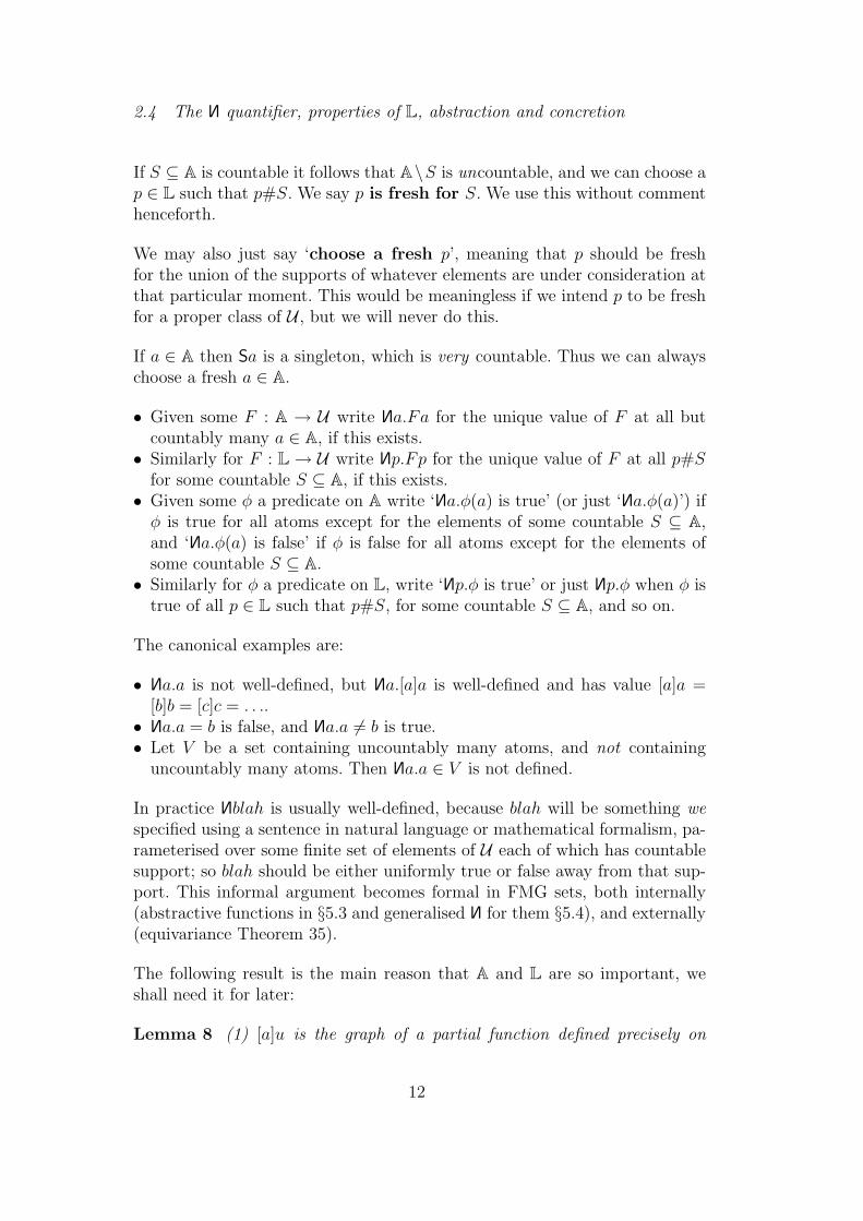
If S ⊆ A is countable it follows that A\S is uncountable, and we can choose ap ∈ L such that p#S. We say p is fresh for S. We use this without commenthenceforth.

We may also just say ‘choose a fresh p’, meaning that p should be freshfor the union of the supports of whatever elements are under consideration atthat particular moment. This would be meaningless if we intend p to be freshfor a proper class of U , but we will never do this.

If a ∈ A then Sa is a singleton, which is very countable. Thus we can alwayschoose a fresh a ∈ A.

• Given some F : A → U write Na.Fa for the unique value of F at all butcountably many a ∈ A, if this exists.

• Similarly for F : L → U write Np.Fp for the unique value of F at all p#Sfor some countable S ⊆ A, if this exists.

• Given some φ a predicate on A write ‘ Na.φ(a) is true’ (or just ‘ Na.φ(a)’) ifφ is true for all atoms except for the elements of some countable S ⊆ A,and ‘ Na.φ(a) is false’ if φ is false for all atoms except for the elements ofsome countable S ⊆ A.

• Similarly for φ a predicate on L, write ‘ Np.φ is true’ or just Np.φ when φ istrue of all p ∈ L such that p#S, for some countable S ⊆ A, and so on.

The canonical examples are:

• Na.a is not well-defined, but Na.[a]a is well-defined and has value [a]a =[b]b = [c]c = . . ..

• Na.a = b is false, and Na.a 6= b is true.• Let V be a set containing uncountably many atoms, and not containing

uncountably many atoms. Then Na.a ∈ V is not defined.

In practice Nblah is usually well-defined, because blah will be something wespecified using a sentence in natural language or mathematical formalism, pa-rameterised over some finite set of elements of U each of which has countablesupport; so blah should be either uniformly true or false away from that sup-port. This informal argument becomes formal in FMG sets, both internally(abstractive functions in §5.3 and generalised Nfor them §5.4), and externally(equivariance Theorem 35).

The following result is the main reason that A and L are so important, weshall need it for later:

Lemma 8 (1) [a]u is the graph of a partial function defined precisely on

12

those c such that c = a or c#u (or equivalently; such that c#[a]u), withvalue (c a) · u where defined.

(2) [p]u is the graph of a partial function defined precisely on q#Su \ Sp (orequivalently; such that q#[p]u), with value Nr.(q r) ◦ (r p) · u.

Proof. We note that by definition, c#[a]u when c#u or c = a, and similarlyq#[p]u when q#Su \ Sp.

(1) Expanding definitions,

[a]u ={〈π(a), π · u〉

∣∣∣ π ∈ Fix(Su \ {a})}

.

The first component π(a) can assume any c#u or c = a, since (c a) ∈Fix(Su \ {a}) for these c.

It remains to show this is functional, i.e. π · u = π′ · u if π(a) = π′(a)and π, π′ ∈ Fix(Su \ {a}). But then π and π′ agree on Su and the resultfollows from the last part of Lemma 3.

(2) Expanding definitions,

[p]u ={〈π · p, π · u〉

∣∣∣ π ∈ Fix(Su \ Sp)}

.

First we show this is functional: suppose π, π′ ∈ Fix(Su \ Sp) and π · p =π′ ·p. By the technical lemma below and Lemma 6, π(c) = π′(c) for everyc ∈ Su. Functionality follows.

We now just need to show that for every q#Su \ Sp, there is someπ ∈ Fix(Su\Sp) such that π ·p = q. Choose some fresh r (taking r#p, q, usuffices) and set π = (q r) ◦ (r p).

2

Lemma 9 (Technical Lemma) Suppose p = [p1, . . .] ∈ L. If π · p = π′ · pthen π(pi) = π′(pi) for every i.

Proof. Lemma 6 proves the permutation action is pointwise. The result isimmediate. 2

We shall write abstractions as u, v. We write the value or concretionof u at some c or q, when this is defined, as u@c or u@q respectively.

The terminology ‘concretion’ is consistent with existing terminology in theFM literature [2, Definition 5.3].

13

Concretion is very useful for specifying functions, since it allows us to ‘choosethe name of the bound variable’. We will use it heavily later.

Lemma 10 (1) [c](u@c) = u when u is an abstraction by an atom and u@cis defined, and ([a]u)@a = u.

(2) [p](u@p) = u when u is an abstraction by an element of L and u@p isdefined, and ([p]u)@p = u.

Proof.

(1) Suppose u = [a]u. By Lemma 8, u@c = (c a) · u and it must be the casethat c#u. By definition

[c](u@c) = [c](c a) · u = (c a) · ([c]u).

We then use the fourth part of Lemma 3, recalling that by definitiona#[a]u and that c#[a]u.

We also observe that (a a) · u = u, so using the previous result([a]u)@a = u follows.

(2) Suppose u = [p]u. By Lemma 8, u@q = (q a) · u and it must be the casethat q#u. By definitions

[q](u@q) = Nr.[q](q r) ◦ (r p) · u = Nr.(q r) ◦ (r p) · ([p]u).

We then use the fourth part of Lemma 3.

2

3 Inductive datatypes

Recall from §2.3 the definitions of cartesian products X × Y , disjoint sumsX + Y , lists X-list, the set of natural numbers N, the classes of atoms andcountable streams of distinct atoms A and L, and so on (for any classes X, Y ⊆U).

Also write

[X]Y for {[x]y | x ∈ X, y ∈ y}.Fix a countably infinite collection of class variable symbols V , V ′, X, andso on. Then expressions of a simple class specification grammar are definedby:

E ::= X, V, V ′ . . . | E × E | [E]E | N | A | E + E | E-list | . . . (3)

14

Say E is closed when it has no class variables. A closed E denotes an actualclass [[E]] ⊆ U in a natural way. For example:

• [[A]] = A.• [[N]] = N, where N is defined in §2.3.• [[E + E ′]] = [[E]] + [[E ′]], where + is defined in §2.3.• [[[E]E ′]] = [[[E]]] [[E ′]] (in this paper we shall only really consider E ∈ {A, L}).• and so on.

Say E is a signature in X when it mentions at most one class variable, andthat variable is X. We abuse notation and write EX for a signature in X.Given EX and E ′X write EE ′X for a signature obtained by substituting E ′Xfor X in EX. For example, (X ×X)(X-list)X = (X-list)× (X-list).

Say permutation acts trivially on u ∈ U when π · u = u for all π. Given aclass X ⊆ U , which may be countable and thus itself an element of U , sayX has a trivial permutation action when permutation acts trivially on everyelement of X.

Lemma 11 If X ⊆ U has a trivial permutation action then [A]X ∼= X and[L]X ∼= X is a canonical way.

Proof. We consider just [A]X; the case of [L]X is similar. Map x to x@a forany a, and x to [a]x for any a. This is well-defined by Lemma 10 and the factthat permutation acts trivially on x and x@a. 2

We need some notation: if S ⊆ U say S is equivariant when

∀x ∈ U , π ∈ PA. x ∈ S ⇔ π · x ∈ S.

Much more on this later in §5.1.

Lemma 12 (1) A and N are equivariant.(2) If X and Y are equivariant, so are X×Y , X +Y , [X]Y , and X-list (and

so on).

Proof.

(1) If a ∈ A then π · a ∈ A, since a permutation π ∈ PA does map atomsto atoms. The result follows since PA is also a group. If n ∈ N then thepermutation action is trivial (that is, π · n = n for all π) and the resultis easy to prove.

(2) All results are by simple calculations. We only give one. Suppose x ∈ Xand y ∈ Y . Then π · [x]y = [π · x]π · y by Lemma 4 and since π · x ∈ Xand π · y ∈ Y , we are done.

15

2

Equivariant classes are easier to work with — we know we can rename atomswithout moving out of the class, see also Lemma 14 below — and sufficientto model syntax-with-binding as we are in the process of demonstrating. Allclasses are assumed equivariant unless stated otherwise.

For some equivariant S ⊆ U write ES for the class denoted by EX interpretedaccording to the list above, where we additionally take X to denote S.

Lemma 13 A signature induces a class ιE (ι for ‘initial’) which is the leastclass such that E(ιE) ⊆ ιE.

Proof. Write E0Xdef= X and Ei+1X

def= E(EX). ιE can be constructed as⋃

i EiX in a standard way (see [10] or [1, Section 10]). We briefly look at the

only unusual aspect of this construction, which is FM(G) abstraction (it turnsout to be quite easy):

Suppose X0 ⊆ X1 ⊆ X2 ⊆ . . . ⊆ U . Then:

(1) [⋃

i Xi]Y =⋃

[Xi]Y : Suppose [x]y ∈ [⋃

i Xi]Y . Then x ∈ Xi for some iand y ∈ Y , so x ∈ [Xi]Y . Conversely if [x]y ∈ ⋃

[Xi]Y then [x]y ∈ [Xi]Yfor some i so x ∈ Xi and [x]y ∈ [

⋃i Xi]Y .

(2) [Y ]⋃

i Xi =⋃

i[Y ]Xi: Similarly.

2

Call ιE an inductively defined datatype. The expression determines itsconstructors.

Three signatures are of particular interest to us by way of prototypical exam-ples:

LncXdef= A + X ×X + A×X LX

def= A + X ×X + [A]X

LdbXdef= N + A + X ×X + X

(4)

ιLnc is an inductive datatype of terms of the λ-calculus without α-equivalence.ιL is an FM datatype of terms up to α-equivalence =α; the lemma

ιL ∼= ιLnc/=α

is easy to prove by induction, but we leave that for α which we construct inthe next section. ιLdb is a de Bruijn datatype for λ-terms in the style of theseminal implementation of abstract syntax up to α-equivalence in Automath[6] by de Bruijn and others.

16

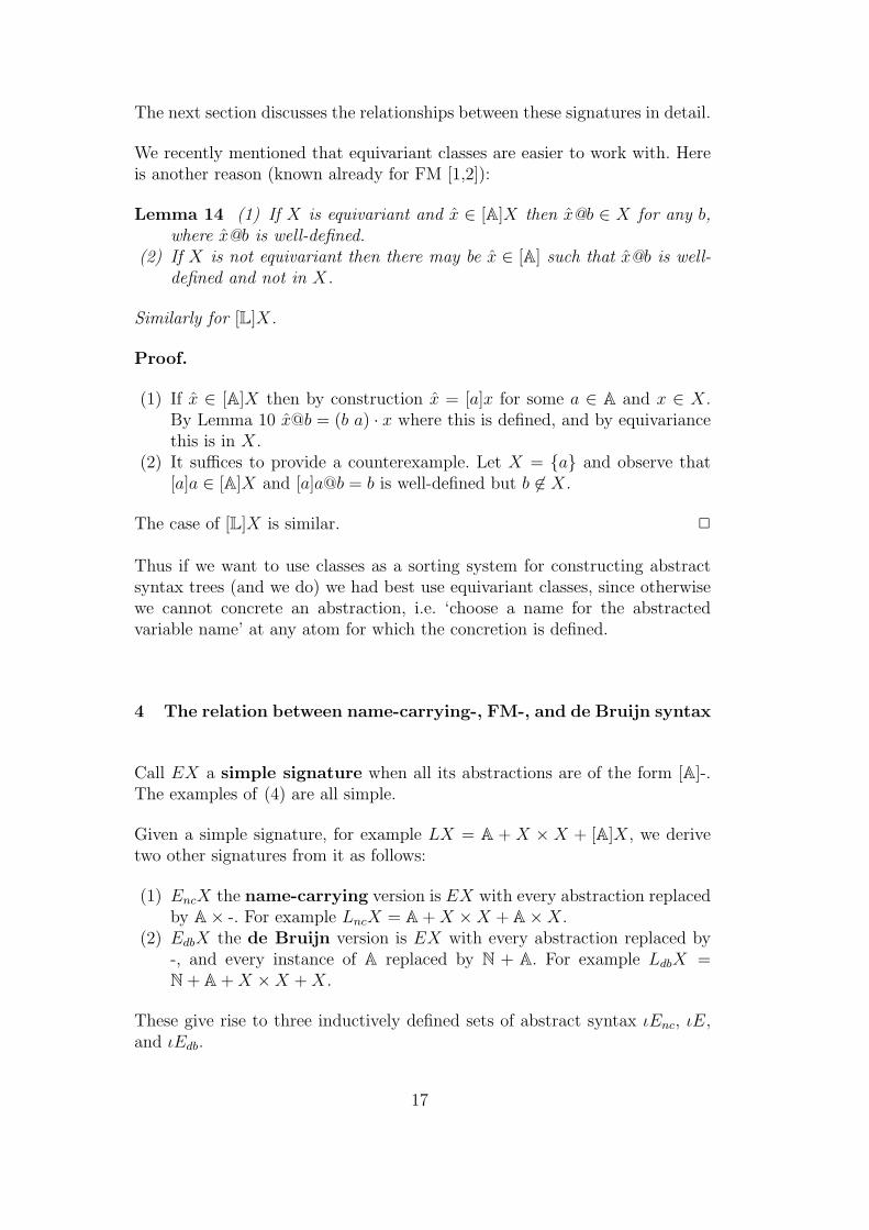
The next section discusses the relationships between these signatures in detail.

We recently mentioned that equivariant classes are easier to work with. Hereis another reason (known already for FM [1,2]):

Lemma 14 (1) If X is equivariant and x ∈ [A]X then x@b ∈ X for any b,where x@b is well-defined.

(2) If X is not equivariant then there may be x ∈ [A] such that x@b is well-defined and not in X.

Similarly for [L]X.

Proof.

(1) If x ∈ [A]X then by construction x = [a]x for some a ∈ A and x ∈ X.By Lemma 10 x@b = (b a) · x where this is defined, and by equivariancethis is in X.

(2) It suffices to provide a counterexample. Let X = {a} and observe that[a]a ∈ [A]X and [a]a@b = b is well-defined but b 6∈ X.

The case of [L]X is similar. 2

Thus if we want to use classes as a sorting system for constructing abstractsyntax trees (and we do) we had best use equivariant classes, since otherwisewe cannot concrete an abstraction, i.e. ‘choose a name for the abstractedvariable name’ at any atom for which the concretion is defined.

4 The relation between name-carrying-, FM-, and de Bruijn syntax

Call EX a simple signature when all its abstractions are of the form [A]-.The examples of (4) are all simple.

Given a simple signature, for example LX = A + X × X + [A]X, we derivetwo other signatures from it as follows:

(1) EncX the name-carrying version is EX with every abstraction replacedby A× -. For example LncX = A + X ×X + A×X.

(2) EdbX the de Bruijn version is EX with every abstraction replaced by-, and every instance of A replaced by N + A. For example LdbX =N + A + X ×X + X.

These give rise to three inductively defined sets of abstract syntax ιEnc, ιE,and ιEdb.

17

We now define functions α and β

ιEncα−→ ιE [L]ιE

β−→ ιEdb (5)

as follows:

To define α, which is out of an inductively defined set, it suffices to define theaction of α on its components. We let α be the identity except on componentswhere EX has [A]X (so that Enc has A×X), in which case α is the abstractionfunction λa, x.[a]x.

For example α : ιLnc → ιL is defined as follows:

• α(a)def= a.

• α(tt′)def= α(t)α(t′).

• α(λa.t)def= λ[a]α(t) (of course the leftmost λ is a term-former of Lnc and

the rightmost λ is a term-former of L).

We define

βtdef= Nl.β′(l, t)

where β′ is defined on L× ιE as follows:

• β′(l, a)def= i if a = li, and β′(l, a)

def= a otherwise.

• β′(l, tt′)def= β′(l, t)β′(l, t′)

• β′(l, λt)def= Na.β′(a :: l, t@a).

It is easy to inductively characterise the kernel ∼ of α on ιLnc:

(1) a∼a.(2) s∼t and s′∼t′ implies ss′∼tt′.(3) Nc.(c a) · t = Nc.(c a′) · t′ implies λa.t∼λa′.t′.

A few examples suffice to convince us that the kernel of α is the relation whichwe would naturally call α-equivalence.

βx is defined as Nl.β′(l, x) where β′ is defined as before. We also state whatto do with countable powersets:

β′(l, U ∈ P≤ω(U))def=

{β′(l, u)

∣∣∣ u ∈ U}

. (6)

Theorem 15 β : ιE → ιEdb described above is an isomorphism.

Proof. It suffices to exhibit the following isomorphisms and observe that β is

18

obtained by applying them repeatedly left-to-right. We only do the first part:

[L](X × Y ) ∼= [L]X × [L]Y [L](X + Y ) ∼= [L]X + [L]Y

[L]N ∼= N [L]B ∼= B[L]P≤ω(X) ∼= P≤ω([L]X) [L]P<ω(X) ∼= P<ω([L]X)

[L](X-list) ∼= ([L]X)-list [L]A ∼= N + A[L][A]X ∼= [L]X

(7)

So β distributes the abstraction [L]- down until it reaches A, at which pointwe obtain N + A.

We consider a selection of cases:

(1) The case X × Y .

u : [L](X × Y ) 7−→ Nl.〈[l]π1(u@l), [l]π2(u@l)〉〈u, u′〉 : ([L]X)× ([L]Y ) 7−→ Nl.[l]〈u@l, u′@l〉

The functions could also be written informally as [l]〈u, u′〉 7→ 〈[l]u, [l′]u〉and 〈[l]u, [l]u′〉 7→ [l]〈u, u′〉. This makes it intuitively obvious that theyare well-defined and mutually inverse.

However, proving this now would be hard; best to wait for later whenin FMG sets we will have powerful results about N(Corollary 39 andTheorem 35). For full proofs, see Theorem 42.

(2) The case N. The functions are given by λn. Nl.(n@l) and λn. Nl.[l]n. SeeLemma 11.

(Note that n ={〈l, n〉

∣∣∣ l ∈ L}

for some n, so n@l = n@l′ for any l

and l′ and Nl.(n@l) is well-defined.)(3) The case of B is similar; indeed, the result holds for any set all of whose

elements have the trivial permutation action.(4) The case P≤ω(X).

U : [L]P≤ω(X) 7−→ Nl.{[l]u

∣∣∣ u ∈ U@l}

U : P≤ω([L]X)) 7−→ Nl.[l]{u@l

∣∣∣ u ∈ U}

It is worth discussing this in a little detail.Suppose we have U : [L]P≤ω(X). Choose l#U ; we know U@l is well-

defined and is a countable set of elements of U . We also know that l#[l]u

for any u ∈ U@l and so that l#{[l]u

∣∣∣ u ∈ U@l}. So the map above is

well-defined (it does not depend on which l#U we choose).Now suppose we have U : P≤ω([L]X). This is a countable collection of

elements so the support of U is the union of the support of its elements;choose some l such that l#u for all u ∈ U ; in particular u@l is well-defined for all u ∈ U . We know that l#[l]

{u@l

∣∣∣ u ∈ U}, so the map

above is well-defined (it does not depend on which l we choose).

19

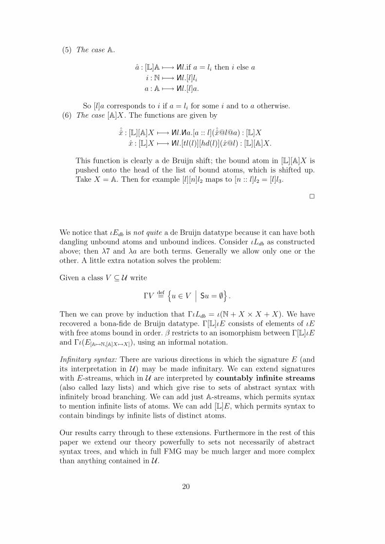
(5) The case A.

a : [L]A 7−→ Nl.if a = li then i else a

i : N 7−→ Nl.[l]lia : A 7−→ Nl.[l]a.

So [l]a corresponds to i if a = li for some i and to a otherwise.(6) The case [A]X. The functions are given by

ˆx : [L][A]X 7−→ Nl. Na.[a :: l](ˆx@l@a) : [L]X

x : [L]X 7−→ Nl.[tl(l)][hd(l)](x@l) : [L][A]X.

This function is clearly a de Bruijn shift; the bound atom in [L][A]X ispushed onto the head of the list of bound atoms, which is shifted up.Take X = A. Then for example [l][n]l2 maps to [n :: l]l2 = [l]l3.

2

We notice that ιEdb is not quite a de Bruijn datatype because it can have bothdangling unbound atoms and unbound indices. Consider ιLdb as constructedabove; then λ7 and λa are both terms. Generally we allow only one or theother. A little extra notation solves the problem:

Given a class V ⊆ U write

ΓVdef=

{u ∈ V

∣∣∣ Su = ∅}

.

Then we can prove by induction that ΓιLdb = ι(N + X × X + X). We haverecovered a bona-fide de Bruijn datatype. Γ[L]ιE consists of elements of ιEwith free atoms bound in order. β restricts to an isomorphism between Γ[L]ιEand Γι(E[A 7→N,[A]X 7→X]), using an informal notation.

Infinitary syntax: There are various directions in which the signature E (andits interpretation in U) may be made infinitary. We can extend signatureswith E-streams, which in U are interpreted by countably infinite streams(also called lazy lists) and which give rise to sets of abstract syntax withinfinitely broad branching. We can add just A-streams, which permits syntaxto mention infinite lists of atoms. We can add [L]E, which permits syntax tocontain bindings by infinite lists of distinct atoms.

Our results carry through to these extensions. Furthermore in the rest of thispaper we extend our theory powerfully to sets not necessarily of abstractsyntax trees, and which in full FMG may be much larger and more complexthan anything contained in U .

20

5 α-equivalence as a mathematical notion

We have related different kinds of inductive datatype for syntax, usingdatatypes of abstract syntax constructed in U by means of proofs based oninduction on the signatures defining the datatypes. This made things nice andconcrete, but it ties us to a concrete notion of signature and to working onlyon sets which happen to be abstract syntax trees.

We can do better: we can jettison both the signatures and their sets of abstractsyntax trees, and define useful functions on general elements u ∈ U with noassumption of inductive structure. We call this type of reasoning ‘syntax-free’.

5.1 Equivariance

Recall that U was defined with an inherently ‘syntax-free’ notion of ‘free namesof u’ given by Su. When Su = ∅, u ‘mentions no names’.

Because this is an important property we give it a fancy name: say u is equiv-ariant when Su = ∅.

We introduced a notion of ‘equivariance’ in §3, for classes (not elements) ofU . The two notions coincide in a suitable sense:

Lemma 16 (1) u is equivariant precisely when ∀π. π · u = u.(2) u is equivariant precisely when ∀y, π. y ∈ u ⇒ π · y ∈ u.

Proof. The second part follows from the first, for suppose π · u = u alwaysand y ∈ u. Recall that π · u = {π · y | y ∈ u}. Then obviously π · y ∈ u.Suppose conversely y ∈ u implies π · y ∈ u. Then π · u ⊆ u. But note that PAis a group, so that y = π−1 · (π · y) ∈ u and u ⊆ π · u.

Now we prove the first part. Suppose u is equivariant. Then π#u always, andby the fourth part of Lemma 3, π · u = u. Now suppose π · u = u always.Then by the second part of Lemma 3, π · Su = Su always, and the only waythis can happen is if Su = ∅. 2

Call a function f equivariant when for all π and x, fπ · x is defined and

π · fx = fπ · x. (8)

Lemma 17 Suppose f ∈ U is the graph of a function. Then Sf = ∅ if andonly if π · fx = fπ · x always — that is, the two notions of equivariance just

21

described, agree where they overlap.

Proof. Suppose f = {〈x, fx〉 | x ∈ dom(f)}. Then

π · f = {〈π · x, π · fx〉 | x ∈ dom(f)}.

Suppose π · f = f . Then we read f(π · x) = π · fx directly off the equationabove. Conversely suppose fπ ·x is always defined and π · fx = f(π ·x). Then〈π · x, π · fx〉 ∈ f . Thus f is defined at π · x, and f(π · x) = π · fx as required.

2

Lemma 18 If f is injective (and thus bijective between imgf and domf) thenf is equivariant if and only if f−1 is equivariant.

Proof. Choose some y = fx. Then π·y = fπ·x and (f−1π·y) = π·x = π·f−1y.2

How does the support of fx relate to the support of x?

Lemma 19 (1) If f is equivariant then Sfx ⊆ Sx and Fix(Sx) ⊆ Fix(Sfx)always.

(2) If f is equivariant and injective then Sfx = Sx.(3) If f(x, y) is equivariant and injective, then Sf(x, y) = Sx ∪ Sy.

Proof.

(1) Suppose f is equivariant, so π · fx = f(π · x) always. Using Lemma 3it is also the case that π · Sfx = Sf(π · x). Now if π#Sx (that is, ifπ ∈ Fix(Sx)) then π · x = x so π · Sfx = Sfx. Since this is valid for anyπ#Sx, it must be that Sfx ⊆ Sx.

(2) Direct from the first part of this lemma, and by the previous result.(3) Suppose π · f(x, y) = f(x, y). By the various properties we assumed, this

happens precisely when π · x = x and π · y = y. The result follows.

2

It is generally useful to assume a function is equivariant: if not we parameteriseuntil we obtain one that is.

A fundamental theorem of model theory is that if we systematically permutethe underlying sets of a model, we obtain a new model in a natural way. Thus

22

we know from very general principles [11] that all functions, if sufficientlyparameterised, must be equivariant.

5.2 A word on support

The reader familiar with FM theory will no doubt recall that support hasanother characterisation in terms of freshness and N. This is indeed the casehere:

Lemma 20 (1) a#x if and only if Nb.(b a) · x = x (‘a is not in x preciselywhen if we rename it to be a fresh b, nothing happens’).

(2) p#x if and only if Nq.(q p) · x = x (‘p is not in x precisely when if werename it to be a fresh q, nothing happens’). .

(3) As a corollary of part 1, x is equivariant precisely when ∀a. a#x.(4) As a corollary of part 2, x is equivariant precisely when ∀p. p#x.

Proof.

(1) Suppose Nb.(b a) · x = x. By part 2 of Lemma 3, also Nb.(b a) · Sx = Sx.Since Sx is countable and all but countably many b satisfy b 6∈ Sx, itfollows by elementary properties of sets and part 1 of Lemma 2 thata 6∈ Sx.

Conversely suppose a 6∈ Sx. Then for each b 6∈ Sx it is the case that(b a) · x = x by part 4 of Lemma 3. The result follows.

(2) Suppose Nq.(q p) · x = x. That means that there is some countable setS such that for all q#S, (q p) · x = x. By part 2 of Lemma 6 we knowSq = {q1, q2, . . .}, and by part 2 of Lemma 2 SS = S. Since all setsconcerned are countable and A is uncountable, there is one (actuallyuncountably many) q#S, p, x such that (q p)·x = x. By part 2 of Lemma 3also (q p) · Sx = Sx and it follows by part 1 of Lemma 2 that p#x.

Conversely suppose p#Sx. By part 3 of Lemma 6, {p1, p2, . . .}∩Sx = ∅and we can use that part again along with part 4 of Lemma 3 to verifythat for any other q#Sx we have (q p) · x = x. The result follows.

(3,4) Left-to-right is immediate since it follows that Sx = ∅. Right-to-left fol-lows since the intersection of any set with the empty set, is empty.

2

Strictly as an aside for the reader who is not surprised by part 3 of the resultabove, because they have seen it in FM, we now show that U is in fact ratherspecial and that in full FMG we cannot take this result for granted.

23

Define an elementwise permutation action on uncountable sets C ⊆ U asπ · C = {π · u | u ∈ C} and let a#C be defined as above by Nb.(b a) · C = C(as is the case in FM). Then we semi-formally (because we have not definedFMG) state:

Lemma 21 Part 3 of Lemma 20 fails in full FMG; there exist C and π suchthat ∀a. a#C is true, but π · C = C is false.

(Of course we have not yet defined FMG set theory, but being a set theory ofsignificant expressive power, it includes uncountable sets and in particular theones we construct in the proof below.) Proof. Choose any p ∈ L and define

Cdef= {π · p | Sπ is finite}.

(Recall that Sπ being finite is equivalent to π(a) = a holding for all but finitelymany atoms. The canonical example of such a π is (a b), and the canonicalexample of a π which is not so is (q p) for some q#p.)

We can easily verify that a#C for any a, but also for any fresh q#p it is thecase that (q p) · C 6= C. 2

In fact, on of our reasons for considering U is that we can build and in-vestigate L and Nin it, and still have part 1 of Lemma 20. We return to thisissue later in §6.2 (fuzzy support in FMG sets); a suitable version of part 4 ofLemma 20 remains valid, see Lemma 43.

First, we return to U because even without fuzzy support, it is by no meanswithout novelty. . .

5.3 Abstractive functions or, syntax-free “quotient by α-equivalence”

Call an equivariant function f purely abstractive when

∀x, x′ ∈ dom(f). fx = fx′ ⇒ ∃π ∈ Fix(Sfx). x′ = π · x.

Write Id :U → U for the identity function mapping u to itself. Later it willbe useful to write IdX for Id restricted to being a partial function on someX ⊆ U .

Lemma 22 (1) Id is abstractive.(2) The abstraction function λa, x.[a]x : A×U → U is purely abstractive.(3) The unique function ! from A to the unit set 1 = {∗} is purely abstractive.(4) The tail-of and head-of functions tl : L → L and hd : L → A are purely

abstractive.

24

(5) The ‘remove atom’ function λU, a.U \ {a} defined for U ∈ P≤ω(A), ispurely abstractive.

(6) The tail-of and head-of functions tl : A-stream → A-stream and hd :A-stream → A are not purely abstractive.

Proof.

(1) If Idx = Idy then x = y and we take π equal to Id (the identity permu-tation; we shall always make it clear which Id we mean).

(2) Suppose [a]x = [a′]x′. Choose some fresh c#a, x, a′, x′. Then [a]x@c =(c a) · x = (c a′) · x′ = [a′]x′ by Lemma 8. It follows using Lemma 3that (a, x) = (a c) ◦ (c a′) · (a′, x′), and we observe by calculations that(a c) ◦ (c a′) ∈ FixS([a]x).

(3) Suppose !a =!b. Well, that always happens, and S∗ = ∅ so it suffices toobserve that (b a) · a = b.

(4) Suppose tl(p) = tl(q). By definitions we know that hd(p)#tl(p) andhd(q)#tl(q), so (hd(p) hd(q)) ∈ Stl(p). Now observe that (hd(p) hd(q)) ·p = q.

Suppose hd(p) = hd(q). Choose some r#p, q. Then observe that(r tl(p)) · p = (r tl(q)) · q. It follows by calculations that p = (r tl(p)) ◦(r tl(q)) · q, and (r tl(p)) ◦ (r tl(q))#hd(p), hd(q).

(5) Suppose U\{a} = U ′\{a′}. Choose some fresh c#a, U, a′, U ′ and observethat (c a) · (U\{a}) = (c a′) · (U ′\{a′}). The result follows similarly tothe case for abstractions.

(6) It suffices to provide a counterexample. Consider s = [a, a, a, a, a, . . .] ands′ = [b, a, a, a, a, . . .]. Then tl(s) = tl(s′) but there is no π such that π ·s′ =s. Similarly consider s and s′′ = [a, b, b, b, b, . . .]. Then hd(s) = hd(s′′) butthere is no π such that π · s = s′′.

2

We shall assume basic properties of permutations, freshness, and support(most notably Lemma 3) without comment henceforth.

α from (5) is not purely abstractive in general. For the example of L and Lnc,observe that α(λa.λb.b) = α(λa.λa.a) but no π exists to make them equal.

This example motivates the following definition:

Call f Barendregt abstractive when for every y in img(f) there is a uniqueFix(Sy)-orbit in f−1y whose support has maximal cardinality. Call an elementof this orbit a Barendregt representative.

Lemma 23 (1) A×A → 1 is Barendregt abstractive with a Barendregt rep-resentative 〈a, b〉 for (any) a 6= b.

(2) A + A → 1 is not Barendregt abstractive because Inl(a) and Inr(a) both

25

map to ∗ and are not related by a permutation π.(3) α from §4 is Barendregt abstractive. A Barendregt representative of

λ[a]λ[a]a is λa.λb.b.

Proof. By simple calculations. A λ-term satisfying the Barendregt variableconvention [12] (that all bound variable names be distinct from each otherand from the free variable names) is precisely what we here call a Barendregtrepresentative. 2

It may be useful to recall that λ[a]λ[b]b = λ[a′]λ[b′]b′ = λ[a]λ[a]a ∈ ιL. How-ever λa.λb.b 6= λa′.λb′.b′ 6= λa.λa.a ∈ ιLnc — all these expressions map to thesame element under α.

Given classes X, X ′, Y, Y ′ ⊆ U and f : X → X ′ and g : Y → Y ′, writef × g : X × Y → X ′ × Y ′ and f + g : X + Y → X ′ + Y ′ for the obviousfunctions on products and sums. For convenience, write Inl(X) ⊆ X + Y forthe left-hand component of the disjoint sum, and similarly for Inr(Y ).

Theorem 24 Continue the notation just established. Then:

(1) If f and g are purely/Barendregt abstractive then f + g mapping Inl(x)to Inl(fx) and Inr(y) to Inr(gy) is purely/Barendregt abstractive.

(2) If f and g are purely/Barendregt abstractive then f × g mapping 〈x, y〉 ∈dom(f)× dom(g) to 〈fx, gy〉 is Barendregt abstractive.

(3) The map λx, y.[x]y is Barendregt abstractive.

As a corollary, the usual α-equivalence quotient on inductive syntax is Baren-dregt abstractive.

Proof.

(1) The Barendregt representative of fx ∈ Inl(X ′) is x, similarly for fy.(2) We consider just the case of products. Given z = 〈zx, zy〉 ∈ X ′× Y ′ let x

and y be Barendregt representatives. Let πx be a permutation in FixSzx

mapping any difference between Sx and Szx to some fresh set of atoms,and similarly let πy ∈ FixSzy map Sy \ Szy to some other fresh set ofatoms. The Barendregt representative of z is 〈πx · x, πy · y〉.

If we accept that the usual α-equivalence quotient on inductive syntax is theidentity on most components, and the abstraction function λa, x.[a]x on A×Xwhere appropriate, then the result follows by induction on the datatype. 2

26

Corollary 25 Second projection on a pair whose first element is in A, writethis π2 = λa, x.x, is Barendregt abstractive. Similarly for second projection ona pair whose first element is in L.

Proof. Combining the previous theorem with the observations about ! whichprecede it. The Barendregt representatives are tuples 〈a, z〉 such that a#z. 2

(Recall that a#z means a 6∈ Sz.)

There is a simple connection between Barendregt abstractive and purely ab-stractive functions:

Lemma 26 A Barendregt abstractive map gives rise to a purely abstractivemap on the subset of its domain consisting of elements with support of maximalcardinality.

Proof. By unpacking definitions. 2

So results of purely abstractive functions can usually be extended to onesof Barendregt abstractive functions, modulo the ‘junk’ of non-Barendregtrepresentatives. Purely abstractive functions are a little easier to work with,so we may prefer to consider them, but this is just for convenience unlessstated otherwise.

Something quite similar to all this is discussed (in the framework of ZF sets) inwell-known work by McKinna and Pollack [13]. The apparatus of abstractivefunctions can be viewed as an abstract account of a phenomenon of which aninstance is treated in [13] as a concrete methodology.

We have defined a new abstract class of functions and shown that a concreteclass of functions are a subset of them. Barendregt abstraction corresponds to‘quotient by α-equivalence’.

For this to be most useful, we need a notion of ‘pick a representative’.

5.4 Generalised Nand Barendregt representatives

Suppose f is a purely abstractive equivariant function and suppose F is an-other equivariant function with dom(F ) = dom(f). Write

F <ab f when for all x ∈ dom(f), SFx ⊆ Sfx.

We argued in the previous subsection that f is a general α-equivalence quotient

27

map. We shall now show that F <ab f is the condition ‘F respects (f)-α-equivalence’.

Theorem 27 For fixed f there is a one-to-one correspondence between F <ab

f and equivariant h such that dom(h) = img(f) and img(h) = img(F ). WriteNfF for the unique h corresponding to F :

• F<abf //

f

��

•

•

Nf F

??��������������

(9)

(If f is Barendregt abstractive, the result still holds, modulo the ‘junk’ ofnon-Barendregt representatives in dom(f).) Proof. Suppose we have F as inthe statement of the theorem. We now define NfF : choose any y ∈ img(f)and pick a representative of y, that is, some x ∈ dom(f) such that fx = y.

Let NfF (y)def= Fx.

We must show this is well-defined. So suppose x′ is any other element suchthat fx′ = y. By the purely abstractive property there exists π ∈ FixSy suchthat x′ = π · x. By equivariance of F we know Fx′ = Fπ · x = π ·Fx. Also byF <ab f we know SFx ⊆ Sfx = Sy and so FixSy ⊆ FixSFx. So π ∈ FixSFx soby Lemma 19 we know Fx′ = π · Fx = Fx as required.

The reverse map is given by composition: given h such that dom(h) = img(f)the corresponding F is h ◦ f .

It remains to show that these maps are inverse, that is

( NfF ) ◦ f = F and Nf (h ◦ f) = h. (10)

(1) For any x, by definition ( NfF )(fx) = F (x′) for some x′ such that fx′ =(fx). Since f is assumed purely abstractive, there is some π#fx suchthat x′ = π · x. But since F <ab f also π#Fx. So Fx′ = π · Fx = Fx.

(2) For any y, by definition Nf (h ◦ f)(y) = (h ◦ f)(x) for some x such thatfx = y. So this is just hy.

2

If img(f) is a two-element set we can interpret it as truth values. We may usethis result for predicates without comment.

For example:

• There is a 1-1 correspondence between maps f out of A × X such that

28

a#f(a, x) always, and maps out of [A]X. This is a known principle of FMtechniques [2, Lemma 6.3].

• If F = λa, z.a#z (restricted to those a and z such that a#z) and f = π2 =λa, z.z then h is the (always true) function λz. Na.a#z. This is the knownaxiom (Fresh) [2, page 8].

• There is a 1-1 correspondence between maps f out of L × X such thatp#f(p, x), and maps out of [L]X.

• . . . and so on.

The construction above is useful because it systematises the treatment ofchoosing representatives and calculating on them, also for sets which may bemuch more complicated than products and projections.

We made a simplifying assumption that f , F , and h be all equivariant. Thisbecomes false the moment they are parameterised over z′, which may containatoms. Those parameters can simply be incorprated into the arguments, or (ifthe reader likes) they can verify that the proofs above do generalise to thismore general situation.

5.5 Freshness

We observed in the last subsection that:

(1) ! : A → 1 is purely abstractive and(2) π2 : A× Z → Z is Barendregt abstractive.

The corresponding generalised Nquantifier N!F and Nπ2F are the well-knownFM N-quantifier, choosing a fresh atom (for a parameter z ∈ Z).

In the rest of this section we concentrate on !:X → 1. In fact π2 : X×Z → Z ismore useful in practice because there the atom is chosen fresh for a parameter ;the arguments below will (obviously) work for π2 as well, just with a smalloverhead of writing ‘Z’ everywhere which we prefer to avoid.

For what sets of X does Nx ∈ X.φ(x) have proper meaning?

Theorem 28 ! : X → 1 is purely abstractive if and only if for all x, x′ ∈ Xthere exists π such that x′ = π · x.

Proof. Suppose ! is purely abstractive. S∗ ∈ 1 = ∅ and Fix∅ = PA. Also!(x) =!(x′) always. Unpacking definitions, for all x and x′ there is some π suchthat π · x = x′.

29

Conversely suppose for all x and x′ that there is some π such that π · x = x′.Clearly this validates the condition for ! to be purely abstractive. 2

Thus ! above is purely abstractive when X consists of a single orbit under PA.

We shall write Nx ∈ X.F (x, z) for Nπ2F , and we say that X has a N-quantifier.In fact it suffices for ! : X → 1 to be Barendregt abstractive (e.g. X = Aω),but then we can restrict attention to the elements of maximal support in X(e.g. L ⊆ X, see below) from which generalised Nchooses its representative.On this subset ! is purely abstractive, thus the situation of the theorem aboveis indeed canonical and useful.

We now show that L satisfies this condition. Recall that p ∈ L is a countablyinfinite stream of distinct atoms.

Lemma 29 For all l, l′ ∈ L there is a π such that l′ = π · l.

Proof. π is given by (l r) ◦ (r l′) for any r#l, l′. 2

(Recall r#l, l′ means ri 6= lj and ri 6= l′j′ for all i, j, j′. Recall from Lemma 7cannot just use (l′ l).)

A and L are minimal and maximal sets for which a N-quantifier exists, in thefollowing sense:

Lemma 30 If X is equivariant and such that for x, x′ ∈ X there always existssome π with π · x = x′, then X is a quotient of L under some subgroup of PA.

Proof. Pick any x ∈ X. This has countable support, so put the atoms in thatsupport in some order and, if the set is finite, pad it with countably manydistinct fresh atoms. Write this stream p ∈ L and declare φ(π · p) = π · x. It isnot hard to verify that provided X is equivariant then φ is well-defined andsurjective, and that its kernel is a subgroup of PA. 2

(Recall we stated we would only be concerned with equivariant classes, in§3.)

We used this technology to study the π-calculus [14] and models of processcalculi with dynamic allocation [15]. FreshML is based on a universe withfinite support, so L does not appear; in a lazy programming version based ona language such as Haskell, L might be useful for foundations.

A benefit of these FM(G) techniques is that they not only account for bindingin the syntax, but also in the semantics, which may very well include functionsand consider infinite behaviour with infinite allocation of names and thus

30

binding by L or variants of it. 5

5.6 Scope extrusion for N

Generalised Nexhibits generalised scope-extrusion. This is the character-istic property of most notions of freshness, that if we choose a fresh name insome context, we can also choose ‘fresher’ for a wider context.

Theorem 31 Suppose f , F , and G are equivariant. Suppose f is abstractive,that domF = domf = X, that imgf = X ′, that imgF = Y , that domG =Z × Y , and that imgG = U .

Suppose F <ab f . Then λz, x.G(z, Fx) <ab IdZ×f , NfF and Nf (λz, x.G(z, Fx))are both well-defined, and

G(z, NfFx) = NIdZ×fG(z, Fx). (11)

In pictures, the left-hand diagram commutes if and only if the right-hand dia-gram commutes:

Z ×XG◦(Z×F ) //

Z×f

��

U

Z ×X ′

G◦(Z×( Nf F ))

=={{{{{{{{{{{{{{{{{{{{{{{{

⇔

Z ×XG◦(Z×F ) //

Z×f

��

U

Z ×X ′

NZ×f (G◦(Z×F ))

=={{{{{{{{{{{{{{{{{{{{{{{{

(12)

Here the Z annotating the arrows actually are the identity IdZ . We use thisnotation without comment henceforth. ◦, as before, denotes function compo-sition. Proof. The proof is just by unpacking definitions. Since these haveaccumulated we give the process in a little detail.

The conditions on domains and images just ensure that all functions are well-defined.

λz, x.G(z, Fx) <ab IdZ × f when for all z and x, SG(z, Fx) ⊆ S〈z, fx〉. ByLemma 19 we know S〈z, fx〉 = Sz ∪ Sfx. Since G is equivariant we knowby Lemma 19 that SG(z, Fx) ⊆ Sz ∪ SFx, and we are done. Therefore thefunctions in question are well-defined.

5 A variant of this not using L was developed and applied by Shinwell and Pitts togive semantics to FreshML, see [5].

31

Now G(z, NfFy) is the value G(z, Fx) at any x such that fx = y and x hasmaximal support. Nfλz, x.G(z, Fx)(z, y) is the value of G(z, Fx′) at any x′

such that fx′ = y and x′ has maximal support and such that Sx′ ∩ Sz isminimal. In particular Fx = Fx′ and we are done. 2

When we work with representatives we do not worry about generating namesfresh for all possible contexts: this is impossible since we do not know a prioriwhat atoms those contexts may contain.

So the above tells us what we always knew; that it does not matter becausewe can always extrude the scope of our choice of fresh name ad hoc. It is notunusual to see results of the form “(ν[a]P ) | Z and ν[a](P | Z) are equivalentup to bisimilarity” (this example is of course taken from the π-calculus and wehave written Z instead of Q to connect the notation to the theorem above).Usually such results are proved on a case-by-case equivalence-by-equivalencebasis, perhaps one day they might be stated as ‘general nonsense’ consequencesof theorems like the ones above.

The following lemma is useful in Theorem 42, and we also used it ‘secretly’when we informally wrote some isomorphisms in Theorem 15.

Lemma 32 Suppose F , and G are equivariant. Suppose that domF = L×X,imgF = Y , domG = L×Y , and imgG = U . Suppose further that F, G <ab π2

(that is if l#x and l#y then l#F (l, x) and l#G(l, y)).

Then λl, x.G(l, F (l, x)) <ab π2 and Nl.G(l, Nl.F (l, x)) = Nl.G(l, F (l, x)) (andthis is all well-defined).

In pictures, the left-hand diagram commutes if and only if the right-hand dia-gram commutes:

L× L×XG◦(L×F ) //

π2◦π2

��

U

X

Nπ2G◦(L× Nπ2F )

<<xxxxxxxxxxxxxxxxxxxxxxx

⇔

L×Xλl,x.G(l,F (l,x)) //

π2

��

U

X

Nπ2λl,x.G(l,F (l,x))

=={{{{{{{{{{{{{{{{{{{{{

(13)

Proof. By the properties of Nwe know it does not matter which Barendregtrepresentatives we use. So suppose we used the representative (l, x) to cal-culate F (l, x) = y so that l#x. Then l#y and we can use (l, y) to calculateG(l, y). The result follows. 2

32

∀x, y. x ∈ y ⇒ y 6∈ A (Sets)

∀x, y 6∈ A. (∀z. z ∈ x ⇔ z ∈ y) ⇒ x = y (Extensionality)

∀x. ∃y 6∈ A. ∀z. z ∈ y ⇒ (z ∈ x ∧ φ) (y not free in φ) (Collection)

(∀x. (∀y ∈ x. [y/x]φ) ⇒ φ) ⇒ ∀x. φ (∈-Induction)

∀x. ∃z. ∀y. y ∈ z ⇒ ∃x′. (x′ ∈ x ∧ y = F (x′)) (Replacement)

∀x, y. ∃z. x ∈ z ∧ y ∈ z (Pairset)

∀x. ∃y. ∀z. z ∈ y ⇒ (∃w ∈ x. z ∈ w) (Union)

∀x. ∃y. ∀z. z ∈ y ⇒ ∀w ∈ z. w ∈ x (Powerset)

∃x. ∃y. y ∈ x ∧ ∀y ∈ x. ∃w ∈ x. y ∈ w (Infinity)

¬wo(A) (AtmLrg)

∀x. ∃S ∈ P(A). wo(S) ∧ S supports x (Fresh)

F any function-class, φ any predicate defined in the logic of FMG. wo(x) is apredicate expressing that there exists a set which is a well-ordering of x.

Fig. 1. Axioms of FMG

6 The underlying theory of sets

6.1 Axioms

FMG sets is a set theory similar to the original FM sets [1], but considerablymore general. So far we have worked in U , a concrete model which is an initialfragment of a standard cumulative hierarchy model of FMG. We now definethe theory.

The logic of FMG sets is First-Order Logic [7,8] with a constant symbol A theset of atoms and a binary predicate ∈ set inclusion.

The axioms of FMG sets are given in Figure 1.

First we make some comments on notation and our choice of axioms:

• We write P(x) for the powerset of x and wo(x) for the predicate “thereexists a set which is a well-ordering of the elements of x”.

• A well-ordering is a well-founded trichotomous relation. A relation R ⊆ x×xis trichotomous when for all z, z′ ∈ x, precisely one of zRz′, z = z′, orz′Rz holds. A relation is well-founded when there exist no infinite strictlydescending chains. The canonical example of a well-ordering is the numerical‘less than or equal’ relation on natural numbers 0, 1, . . .. This ceases to be

33

well-founded if we add negative numbers, and is not trichotomous if wemove to the complex integers a + ib, ordered by the size of their modulous.

• In (Extensionality), (Union), and (Powerset) we could use ⇔ in the axioms,but the system is equivalent.

In the case of (Extensionality) this is by the rules of equality in first-orderlogic.

In the cases of (Union) and (Powerset) we can use the axioms as statedto deduce that some set containing the union or powerset, and then use(Collection) to deduce that the collection which is the union or powerset,is a set.

It is a general fact about this style of axiomatisation of set theory that theimpact of most axioms is just to ensure that there are enough sets around;(Collection) then puts on the final touches, so to speak.

Where does FMG stand with respect to FM sets?

FM sets has a notion of a ‘small set of atoms’. The Nquantifier means precisely‘for all but a small set of atoms, . . . ’.

Originally [1,16] ‘small’ was equal to ‘finite’. We also took A to be countablyinfinite, so the Na.φ(a) means ‘for countably many a, φ(a)’. It was folklorethat we could just have well have taken A to be uncountable; the importantpoint was what we might call the ‘size of small’.

U took ‘small’ to mean ‘countably infinite’. Of course we also insist A beuncountable, so that Nis not degenerate.

FMG set theory generalises this further to:

‘small’ means ‘internally well-orderable’.

This is very nice because (rather unexpectedly, perhaps) it makes no commit-ment to actual size; FMG sets is consistent with any of the following axioms:“Small is finite”, “small is countable”, and “small is ωω” (here ω is the firstuncountable ordinal).

If we add the first as an axiom in FMG sets we recover FM sets. The secondpossibility gives a set theory suitable for containing U in its standard cumula-tive hierarchy model. Further possibilities give theories with increasingly largesmall sets of atoms. Or, we can add no extra axiom and consider FMG withno further assumptions.

As we mentioned in the Introduction, ‘small equals well-orderable’ seems theright choice, because it gives enough isomorphisms to rename atoms:

Lemma 33 For any two well-orderable sets α and β, one is in bijection with

34

a subset of the other.

Proof. See [4, Lemma 6.3]. 2

We obtain permutations from these injections and we can use them to renameatoms to be fresh. This turns out in practice to be the property we need asmall set to satisfy: that the set can always be renamed to be fresh (and theproperty of a large set is that this is not the case).

Write ZF for Zermelo-Fraenkel set theory (a classic mathematical foundation[3,4]).

Theorem 34 FMG set theory is consistent relative to ZF. In addition, for anyordinal α FMG set theory with an additional axiom ‘small is α’ is consistentrelative to ZF.

Proof. The first part is a corollary of the second, so we concentrate on thesecond part.

FMG is just a theory in first-order logic (whose axioms are presented for thedelectation of future generations in Figure 1). To prove consistency of anytheory in first-order logic it suffices to exhibit a model. Because of fundamen-tal limits to logic [17, Proposition VI] a model, i.e. consistency, cannot beexhibited in any absolute sense, but only relative to assuming the consistency,i.e. the existence of a model, of another theory.

So suppose we have a model of Zermelo-Fraenkel set theory. We construct acumulative hierarchy model of FMG set theory (with ‘small = countable’; thegeneralisation to any α is very easy) as a subclass of the elements of that model.This suffices to prove relative consistency. We only sketch the construction,since this is an entirely standard method found often in the literature [18,19].

Choose any uncountable ZF set for A. Define a hierarchy of increasing sub-classes by:

(1) V0 = A.(2) Vα+1 is the set of subsets of Vα with small support, union with Vα.

A set x has small support when there exists a countable set of atoms S suchthat if π ∈ FixS then π · x = x.

Then the model of FMG is V =⋃

i Vi, the union of the Vi. Set-membership inthe model is interpreted by set-membership in V .

The proof that this is a model of the axioms of FMG sets given in Figure 1 is

35

long but routine. We only sketch it here:

(1) (Sets) is valid by construction; everything in V is an atom or a set of(sets of (sets of . . . )) sets of atoms.

(2) (Extensionality) is inherited from ZF.(3) (Collection) is proved by induction on the size of φ, a formula in the logic

of FMG (the same logic in which the axioms are expressed).(4) (∈-Induction) is by the inductive nature of the construction.(5) (Replacement) is inherited from ZF.(6) (Pairset) and (Union) likewise.(7) (Powerset) is inherited from ZF, bearing in mind that we only take the

sets with countable support.(8) (Infinity) is inherited from ZF.(9) (AtmLrg) is by the fact that any set encoding a well-ordering of A is

invariant only under the identity permutation on A.(10) (Fresh) by the construction of the cumulative hierarchy, which only takes

sets with small support.

2

In the presence of an axiom that ‘small’ is (at least) ‘countable’ we can inter-pret U in this cumulative hierarchy and abstractions, as promised, are imple-mentable as the collection defined in §2.1, which is now also a set.

The permutation action π · x is defined by ε-induction starting at atoms andpointwise on sets, thus:

π · a = π(a) π · x = {π · x′ | x′ ∈ x}

The following result corresponds in FMG to the same result in FM (see forexample [2, Lemma 4.7] and [20, Proposition 2]):

Theorem 35 (Equivariance) (1) If φ(x1, . . . , xn) is a predicate in FMGthen

φ(x1, . . . , xn) ⇔ φ(π · x1, . . . , π · xn)

is always provable.(2) If f(x1, . . . , xn) is a function-class specified in FMG then

π · f(x1, . . . , xn) = f(π · x1, . . . , π · xn).

Proof.

36

(1) By induction on the language of FMG (just like the similar result for FM[1,2]). The important base cases are π · A = A and x ∈ y if and only ifπ · x ∈ π · y by the pointwise definition of permutation.

(2) A function-class is merely a predicate specifying its graph. We use thefirst part to deduce

φ(x1, . . . , xn, z) ⇔ φ(π · x1, . . . , π · xn, π · z)

and the result follows immediately.

2

In words:

Any predicate specified in (the logic of) FMG sets is equivariant over itsarguments, and so is any function-class.

FMG set theory is a set theory so models of FMG sets are closed underpowersets, not just countable powersets as U was (nota bene: FMG powersetsdo not take all the subsets of the ambient foundation, only those with smallsupport). FMG sets displays a richness of structure far exceeding U .

6.2 Lifting constructions in U to the set theory

A is a set in FMG, identified by the predicate - ∈ A. So are the naturalnumbers, pairs, cartesian products, disjoint sums, lists, streams, and theirconstructors such as 〈x, y〉, Inl(x), Inr(x), and so on; the constructions arejust as in §2.3.

In particular we recall that 〈x, y〉 can be implemented in sets as {{x}, {x, y}}.

L and A are now sets. Function-sets are built as their graphs as is standard.PA is identified by:

PAdef=

{f : A → A

∣∣∣ f bijective}

.

Lemma 36 (1) π′ · π = ππ′.(2) Any permutation π ∈ PA is the identity off some well-orderable set of

atoms.

In the first part, π′ ·π denotes π′ (the permutation) acting on π (the function-set). ππ′ denotes the function-set expressing the graph of the permutationπ′ ◦ π ◦ π′−1. Proof.

37

(1) We observe that π′ acts on the graph of π by acting on the atoms withinit; it is a fact of group theory that conjugation does the same.

(2) If S supports π then S contains every atom such that π(a) 6= a (sinceotherwise we could permute π(a) to something else). Since π is a set, ithas well-orderable support. The result follows.

2

If S ⊆ A write

Fix(S) for {π ∈ PA | ∀a ∈ S. π(a) = a}.

We say

S supports x when ∀π ∈ PA. π ∈ Fix(S) ⇒ π · x = x.

Finally define

Sx by⋂ {

S ⊆ A∣∣∣ ∀π. π ∈ Fix(S) ⇒ π · x = x

},

(though the next result shows this is not as useful as we might imagine).

Lemma 37 (1) If S and T support x and are well-orderable, then so is S∩T .(2) Sx does not necessarily support x.

Proof.

(1) Suppose S and T support x and suppose π′ fixes just S∩T . Let U = S\T .By (AtmLrg) A is not well-orderable and since U certainly is, we canchoose some U ′ disjoint from S, T , U , and a supporting set for π′.

Since U and U ′ are well-orderable and the same size, there is an idem-potent permutation π = π−1 bijecting U with U ′ and fixing all otheratoms (swap the ith elements of U and U ′, for arbitrary but fixed well-orderings). Now π fixes T so π · x = x. Now π′ fixes S ∩ T and also U ′ soπ ◦ π′ ◦ π which is equal to π′π (since π = π−1) fixes π · (S ∩ T ) ∪ π · U ′

which includes S. Therefore π ◦ π′ ◦ π · x = x. Applying π to both sidesand simplifying we deduce that π′ · x = x as required.

(2) It suffices to consider the example of Lemma 21.

2

So here, at least, FMG is not as tractable as FM (or U)! The notion of asupporting set is still valid and useful, and we may still intersect supportingsets to obtain smaller supporting sets — but if we do this infinitely often wemay ‘miss an infinitesimal bit of support’.

When Sx does not support x, say x has fuzzy support. When Sx does

38

support x, say it has sharp support.

U identifies a convenient subset of the FMG universe which exhibits induc-tive datatypes of abstract syntax with infinitary binding, but still has sharpsupport.

Lemma 38 (1) Permutations have sharp support, and Sπ = {a | π(a) 6= a}.(2) a ∈ A and p ∈ L have sharp support, and Sa = {a} and Sp = {p1, p2, . . .}.

(As before) π · p = [π · p1, . . .].(3) If x has sharp support, then so does π · x.(4) If S supports x then π · S supports π · x. As a corollary, Sπ · x = π · Sx.

Proof.

(1) A permutation is represented as a set by its graph; e.g. (a b) ={〈a, b〉, 〈b, a〉, 〈c, c〉, 〈d, d〉, . . .}. It is not hard to verify the requisite proper-ties, recalling that π acts pointwise on sets and 〈x, y〉 is just {{x}, {x, y}}.

(2) By concrete calculations.(3) The property of being a supporting set can be expressed by a predicate φ

in FMG. The result follows by part 1 of Theorem 35 (a proof by concretecalculations is also possible). The second part follows by calculations, ordirectly by part 2 of Theorem 35.

2

As a matter of notation write

x#y when ∃S, T. S supports x ∧ T supports y ∧ S ∩ T = ∅.

The reader may like to compare this with the corresponding definition from§2.1, which was x#y when Sx∩ Sy = ∅. The difference is of course due to thepossibility of fuzzy support; if x and y have sharp support the two versionsbecome equivalent.

The following result is a useful corollary of Equivariance (it also generalisesLemma 19, which there was proved for U by concrete calculation):

Corollary 39 (1) If S supports x1, . . . , xn and f is a function-class specifiedin the language of FMG with parameters amongst the xi, then S supportsf(x1, . . . , xn).

(2) As a corollary, if f(x1, . . . , xn) is a function-class in FMG with parame-ters x1,. . .xn, then if p#x1, . . . , xn then p#f(x1, . . . , xn).

Proof. It suffices to apply the second part of Theorem 35. 2

In words:

39

Any function-class specified in (the logic of) FMG sets, does not createsupport.

We verify that a suitable version of Lemma 3 is still valid:

Lemma 40 (1) If S supports x then π · S supports π · x. Also, π · (Sx) =S(π · x).

(2) x#[x]y.(3) If π#x then π · x = x.(4) If π(a) = π′(a) for all a ∈ S for some S supporting x, then π · x = π′ · x.

Proof.

(1) Direct from Theorem 35 for the predicate ‘supports’ and the function ‘S’.(2) From Lemma 41.(3) π#x when π fixes a set supporting x. The result follows.(4) By definition of supporting set.

2

Abstractions [x]y are defined much as in §2.1, but we must assume x has sharpsupport, and protect against the possibility that y has fuzzy support by notusing Sy:

[x]ydef= {〈π · x, π · y〉 | ∃S. S supports y ∧ π#S\Sx}.

Lemma 41 (1) π · ([x]y) = [π · x](π · y) holds.(2) If x has sharp support then S supports y if and only if S\Sx supports

[x]y.

Proof.

(1) By part 2 of Theorem 35.(2) In essence identical to the proof of the case for abstractions of part 4 of

Lemma 3, we sketch half of it in full:We can prove by calculation that {π | ∃S. S supports y ∧ π#S\Sx} is

a group.Suppose x has sharp support and S supports y. Suppose π ∈ Fix(S\Sx).

Then

π·[x]y ={〈π′ · (π · x), π′ · (π · y)〉

∣∣∣ ∃S ′, π′. S ′ supports π · y ∧ π′ ∈ Fix(S ′\π · Sx)}

={〈π′′ · x, π′′ · y〉

∣∣∣ ∃S ′, π′′. S ′ supports y ∧ π′′ ∈ Fix(S ′ \ Sx)}

= [x]y.

Now suppose S supports [x]y and suppose π ∈ Fix(S ∪ S(x)). Then

40

(πx, πy) ∈ [x]y. The result follows from the fact that {π | ∃S. S supports y∧π#S\S(x)} is a group.

2

(It does not seem fruitful to consider [x]y when x does not have sharpsupport.)

The maps between ιE, ιEnc, and ιEdb, can also be constructed as before.

It is not hard to verify that Lemma 10 transfers unchanged to FMG. Thediscussions of purely abstractive and Barendregt abstractive functions, N, andfreshness, transfer almost word-for-word.

6.3 Abstractions commute with pairsets, powersets, and more

Theorem 15 generalises beautifully in FMG. We give just the case for cartesianproduct, and also full function spaces and powersets (not just countable ones,as we did in Theorem 15).

Theorem 42 (1) [L](X × Y ) ∼= [L]X × [L]Y .(2) [L](Y X) ∼= [L]Y [L]X .(3) [L]P(X) ∼= P([L]X).

Similarly for A, e.g. [A](Y X) ∼= [A]Y [A]X .

Proof. We consider just the cases for L; the cases of A is simpler.

(1) We map

u ∈ [L](X × Y ) to Nl.〈[l]π1(u@l), [l]π2(u@l)〉〈u1, u2〉 ∈ ([L]X)× ([L]Y ) to Nl.[l]〈u1@l, u2@l〉

These maps are well-defined since it is easy to use Corollary 39 and part 2of Lemma 40 to deduce l#〈[l]π1(u@l), [l]π2(u@l)〉 and l#[l]〈u1@l, u2@l〉.

We now verify that these maps are self-inverse. By Lemma 32 it sufficesto check that (for one suitably fresh l)

u = [l]〈([l]π1u@l)@l, ([l]π2u@l)@l〉〈u1, u2〉 = 〈[l]π1

([l]〈u1@l, u2@l〉

)@l, [l]π2

([l]〈u1@l, u2@l〉

)@l〉.

This follows easily, using Lemma 10.

41

(2) We map

f ∈ [L](Y X) to λx. Nl.[l]((f@l)(x@l))

f ∈ ([L]Y )[L]X to Nl.[l](λx.f([l]x)@l)

We must check these maps are well-defined. Suppose f and x aregiven. Choose some l#f , x. Then f@l and x@l are well-defined andl#[l](f@l)(x@l). Conversely suppose f is given. Choose some l#f . Thenl#f([l]x) so f([l]x)@l is well-defined and l#[l]λx.f([l]x)@l.

We now verify that these maps are self-inverse. By Lemma 32 it sufficesto check that (for one suitably fresh l)

(f@l)x =([l](f@l)(([l]x)@l)

)@l f x = [l]([l](λx.f([l]x)@l)@l)(x@l)

This follows easily, making heavy use of Lemma 10.(3) This is a corollary of the previous lemma, taking Y = B and observing

that [L]B is naturally isomorphic to B, see Theorem 15.In full, the maps are given by:

U ∈ [L]P(X) to U ′ def= Np.

{[p]u

∣∣∣ u ∈ U@p}

U ⊆ [L]X to U ′ def= Np.[p]

{u@p

∣∣∣ u ∈ U ∧ p#u}

.

2

This result is important because it enables us to drop the condition im-plicit in the construction of U of considering just countable powersets. SinceP(X) is strictly larger than X, and similarly Y X is strictly larger than Y andX (provided Y and X have more than two elements), and they not inheritany inductive structure, this theorem is one way of making formal that ourtreatment of names and bindings in FMG is strictly more general than thestandard model given by abstract syntax trees.

This extension to function-sets is also useful, e.g. for the existence of a monadin the semantics of FreshML used to prove the language correct, and for equal-ities used in understanding models of behaviour [21,15].

6.4 An algebraic version

We give an alternative presentation of U and FMG in algebraic style. Fix aparticular uncountable set A. Let PA be permutations of A with countablesupport. Then a Nominal FMG set (where small=countable) is:

∀x. Id · x = x ∀π, π′, x. π · π′ · x = π ◦ π′ · x∀x. Np. Nq.(p q) · x = x ∀x. Na. Nb.(a b) · x = x.

(14)

42

Here Na.φ means that φ holds of all but a countable set of atoms, and Np.φmeans that φ holds of countable lists of distinct atoms whose atoms may beall but a countable set of atoms.

It is easy to verify that an equivariant FMG set (for any given model of FMGsets), or an equivariant subclass of U , is a Nominal FMG set. If we need moreatoms we just take A to be larger and π ∈ PA to have any support strictlysmaller than the size of A.

Lemma 43 (1) L is a nominal FMG set with small=countable.(2) If x ∈ X is such that l#x for all l ∈ L then π · x = x always.

Proof.

(1) By part 2 of Lemma 38.(2) By part 1 of Lemma 38 we know that π permutes only countably many

atoms. Let S support x (we use it in a moment). We choose some l′

suitably fresh for π, S and deduce that π · (l′ l) · x = π · x. By part 3 ofLemma 38 we conclude that π · (l′ l) · x = x.

2

It is now easy to see that if we know that small=X where X is some cardinal-ity, then similar results hold for streams of distinct atoms of length an ordinalwith cardinality X. This is the correct generalisation of the FM principle that∀a. a#x implies x is equivariant.

7 Future work

Infinite binding arises in behavioural models of reactions: for example, if

Pdef= ν[a]aa then the π-calculus process !P is behaviourally equivalent to the

‘infinitary’ process P | P | . . . [22]. Also, if ω3def= λx.xxx then the λ-calculus

process ω3ω3 is αβ-equivalent to the ‘infinitary’ process (((. . . ω3)ω3)ω3)ω3.This equivalence can be made formal by considering a behavioural notion ofmodel, which can display infinite structure even though the trace of any par-ticular behaviour may be finite. One such structure is considered by Montanariet al [23] which we can view as a de Bruijn-based model of behaviour whichmay generate fresh names, whose main interest is in powerful optimisationswhich merge nodes identical except for permutations of names.

If name-binding is modelled by FM-style abstractions, there is a need for infi-nite FM-style abstraction in the model of behaviour. 6 We have proposed one

6 Since this paper was submitted for publication, a paper has been published de-

43

method of obtaining this effect. We have examined the proof-principles whichseem useful on these objects, and by progressive abstraction we have formalisedand generalised them to obtain notions such as ‘abstraction and concretion byinfinitely many atoms’, ‘abstractive functions’, ‘Barendregt representatives’,‘generalised N’, and we have described some nice results describing their prop-erties.

U has an interesting capture-avoiding substitution action given as follows:

a{a 7→u} = u b{a7→u} = b V {a7→u} ={v{a7→u}

∣∣∣ v ∈ V}

([v′]v){a7→u} = [v′](v{a7→u}) Sv′ ∩ Su = ∅(15)

(Recall that an element of U is either an atom a, a countable set V , or anabstraction [v′]v, and that for any abstraction there is a choice of v′ and vforming that abstraction such that Sv′ ∩Su = ∅; thus this is a total function.)

Since β-reduction is given in the λ-calculus, this suggests that we might usethe FM model of abstraction to obtain models of the λ-calculus that are notScott domains, and with a set-theoretic flavour. The obstacle to this idea isthat we do not know what application is. This is current work.

References

[1] M. J. Gabbay, A theory of inductive definitions with alpha-equivalence, Ph.D.thesis, Cambridge, UK (2000).

[2] M. J. Gabbay, A. M. Pitts, A new approach to abstract syntax with variablebinding, Formal Aspects of Computing 13 (2001) 341–363.

[3] J. Bell, M. Machover, A course in mathematical logic, North-Holland, 1977.

[4] P. T. Johnstone, Notes on logic and set theory, Cambridge University Press,1987.

[5] M. R. Shinwell, A. M. Pitts, On a monadic semantics for freshness, TheoreticalComputer Science 342 (2005) 28–55.

[6] N. G. de Bruijn, Lambda calculus notation with nameless dummies, a tool forautomatic formula manipulation, with application to the church-rosser theorem,Indagationes Mathematicae 5 (34) (1972) 381–392.

[7] J. Barwise, An introduction to first-order logic, in: J. Barwise (Ed.), Handbookof Mathematical Logic, North Holland, 1977, pp. 5–46.

scribing a semantics for FreshML which approximates this in a category with aFM-style monad representing finitely but unboundedly many abstractions [5].

44

[8] D. van Dalen, Intuitionistic logic, in: D. Gabbay, F. Guenthner (Eds.),Handbook of Philosophical Logic, 2nd Edition, Volume 5, Kluwer, 2002, pp.1–114.

[9] J. B. Fraleigh, A First Course in Abstract Algebra, Addison-Wesley, 1994.

[10] L. C. Paulson, A fixedpoint approach to implementing (co)inductive definitions,in: CADE-12: Proceedings of the 12th International Conference on AutomatedDeduction, Springer-Verlag, London, UK, 1994, pp. 148–161.

[11] J. Truss, Permutations and the axiom of choice, in: H. R.Kaye (Ed.),Automorphisms of first order structures, OUP, 1994, pp. 131–152.

[12] H. P. Barendregt, The Lambda Calculus: its Syntax and Semantics (reviseded.), Vol. 103 of Studies in Logic and the Foundations of Mathematics, North-Holland, 1984.URL http://www.andrew.cmu.edu/user/cebrown/notes/barendregt.html

[13] J. McKinna, R. Pollack, Some lambda calculus and type theory formalized,Journal of Automated Reasoning 23 (3-4) (1999) 373–409.

[14] M. J. Gabbay, The π-calculus in FM, in: F. Kamareddine (Ed.), Thirty-fiveyears of Automath, Kluwer, 2003, pp. 80–149.

[15] M. J. Gabbay, Fresh graphs, submitted (November 2003).

[16] M. J. Gabbay, A. M. Pitts, A new approach to abstract syntax involving binders,in: 14th Annual Symposium on Logic in Computer Science, IEEE ComputerSociety Press, Washington, 1999, pp. 214–224.

[17] K. Godel, On formally undecidable propositions in principia mathematica andrelated systems i, available online in translation by Martin Hirzel (1931).

[18] N. Brunner, 75 years of independence proofs by fraenkel-mostowski permutationmodels (1996).

[19] K. Kunen, Set Theory: An Introduction to Independence Proofs (Studies inLogic and the Foundations of Mathematics), Elsevier, 1980.

[20] A. M. Pitts, Nominal logic, a first order theory of names and binding,Information and Computation 186 (2003) 165–193.

[21] M. R. Shinwell, A. M. Pitts, M. J. Gabbay, FreshML: Programming withbinders made simple, in: Eighth ACM SIGPLAN International Conference onFunctional Programming (ICFP 2003), Uppsala, Sweden, ACM Press, 2003, pp.263–274.

[22] R. Milner, J. Parrow, D. Walker, A calculus of mobile processes, II, Informationand Computation 100 (1) (1992) 41–77.

[23] U. Montanari, M. Pistore, History-dependent automata, Tech. Rep. TR-98-11,University of Pisa (5, 1998).

45