A General Methodology to Predict the Linear Rheology of BranchedPolymers

E. van Ruymbeke,*,† C. Bailly,‡ R. Keunings,§ and D. Vlassopoulos†,|

FORTH, Institute of Electronic Structure & Laser, Heraklion, Crete, Greece, Unite de Physique etChimie des Hauts Polyme`res, UniVersitecatholique de LouVain, LouVain-la-NeuVe, Belgium, CESAME,UniVersitecatholique de LouVain, LouVain-la-NeuVe, Belgium, and Department of Materials Science &Technology, UniVersity of Crete, Heraklion, Crete, Greece

ReceiVed February 28, 2006; ReVised Manuscript ReceiVed July 7, 2006

ABSTRACT: We present a general coarse-grained model for predicting the linear viscoelasic properties of branchedpolymers from the knowledge of their molecular structure and three viscoelastic parameters, i.e., the Rouse timeof an entanglement segment, the plateau modulus, and the entanglement molecular weight. The model uses theingredients of the tube-based theories of McLeish and co-workers, and its implementation is based on a time-marching algorithm; this conceptual approach was already successfully applied to linear and star polymers, andit is appropriately modified here to account for more complex branched architectures, within the framework ofdynamic tube dilation (using the criteria of Graessley). Whereas the molecular physics behind this model is thewell-established hierarchical tube-based motion, the new element is a different macromolecular coordinate systemand account of the branch points diffusion. With proper account of polydispersity, successful description of awide range of rheological data of H and pompom polymers is obtained, with the use of the dilution exponentR) 1 and the parameterp2 ) 1. The proposed methodology thus represents a generic approach for predicting thelinear rheology of branched polymers.

I. Introduction

Branched polymer rheology represents a very active field ofresearch with important challenges, both from the scientific andtechnological viewpoints. Recent progress in this field wastriggered by the advances in the tube-model theories1-7 and theavailability of well-defined model polymers.8-12 It is now knownthat branched polymers relax hierarchically.13-18 In other words,entanglements belonging to topologically different parts of themacromolecule (branches or backbone or different layers) relaxin a certain sequence, obeying seniority rules according to whichthe outermost parts of the molecule (those with free danglingends) relax first and the innermost ones last; the stress is fullyrelaxed only after the slowest segments have lost the memoryof their initial orientation. For example, for the case of anH-polymers,14,19 the simplest hierarchical branched structurewith a linear connector chain linking two grafted linear chains,the relaxation sequence is as follows: the end-grafted chainsrelax first (via starlike relaxation, as described by the Milner-McLeish model20,21) while the backbone remains frozen, andeventually the backbone relaxes by reptation. The analysis iscarried out in the context of dynamic tube dilation (DTD),20-23

according to which the relaxed branches act as solvent for theyet-unrelaxed backbone. However, the relaxed branches repre-sent an extra friction for the branch point; the effect on theoverall relaxation process is accounted for by the branch pointdiffusion, which has to precede the backbone reptation. Theincorporation of the branch point diffusivity includes anunknown parameter,p2.24-26

Recently, a time-marching algorithm was developed to pre-dict the linear viscoelastic properties of mixtures of linear and

star polymers, as well as asymmetric star polymers.27 It isbased on the tube model predictions of the fluctuations andreptation processes, which proceed simultaneously, but withdifferent probabilities, without any imposed time scale sep-aration; the solvent effect due to relaxed segments is treatedas a constraint release effect based on the approach ofGraessley.28-30 The model provides excellent predictions of thelinear rheology for a wide range of linear polymer mixturesand asymmetric stars.27 More importantly, in the latter case thereis no need to invoke thep2 parameter (as there is no artificiallyimposed time scale separation), thus avoiding the relatedcontroversy.24-26,31,32

On the basis of this recent success, and keeping in mind theongoing concerns about the value of thep2 parameter for dif-ferent branched polymers,24-26,31,32as well as on the availabilityof accurate data sets with a variety of model branched polymers,we decided to expand this time-marching methodology toarchitecturally complex macromolecules. This is the scope ofthe present contribution, which focuses on the prediction of thelinear rheology of pompom and (their special case) H-polymers,and compares with existing relevant experimental data.

The paper is organized as follows: After this introduction,we present in section II the main ingredients of the theoreticalmodeling, including the macromolecular coordinates, relaxationmodes, dilution and polydispersity effects. Then, in section IIIwe present and discuss the predictions of the model, and inparticular we compare them against published experimental datafor model H and pompom polymers. Finally, the main conclu-sions and consequences from this work are summarized insection IV.

II. Theoretical Modeling

II.1. Equilibrium State and Equilibrium Lengths. Asalready mentioned, he treatment of the friction around a branchpoint, due to the relaxed branches, is very important for thecalculation of the fluctuations times of the backbone segments.

* Corresponding author. E-mail: evelynvr@iesl.forth.gr.† FORTH, Institute of Electronic Structure & Laser.‡ Unite de Physique et Chimie des Hauts Polyme`res, Universite´ catholique

de Louvain.§ CESAME, Universite´ catholique de Louvain.| Department of Materials Science & Technology, University of Crete.

6248 Macromolecules2006,39, 6248-6259

10.1021/ma0604385 CCC: $33.50 © 2006 American Chemical SocietyPublished on Web 08/10/2006

Dow

nloa

ded

by U

NIV

CA

TH

OL

IQU

E D

E L

OU

VA

IN o

n O

ctob

er 1

5, 2

009

| http

://pu

bs.a

cs.o

rg

Pub

licat

ion

Dat

e (W

eb):

Aug

ust 1

0, 2

006

| doi

: 10.

1021

/ma0

6043

85

Likewise, defining the effective backbone equilibrium length(after the relaxation of the branches), about which the real lengthof the backbone fluctuates, is also of great significance for theproper analysis of branched polymer relaxation. As alreadymentioned, DTD suggests that the polymer fraction alreadyrelaxed will act as a solvent for the relaxation of the remainingoriented part of the polymer. Therefore, the equilibrium stateof the polymer evolves in time as a function of the unrelaxedpart of the polymer,Φ(t):20,21,23

whereR is the dilution exponent,Me(t), the effective molecularweight between two entanglements,a(t), the effective tubediameter andLeq(t), the effective equilibrium length of asubchain at timet if its length is equal toLeq(0) at timet ) 0.According to these equations, after the branches of a pompommolecule have relaxed, their effective equilibrium length isreduced in exactly the same way as the effective equilibriumlength of the backbone or of the inner part of the backbone.This is a consequence of the fact that both branches andbackbone are assumed to “see” the same environment:

whereLeq,branchandLeq,inner backboneare the equilibrium length ofone branch and of the half-inner part of the backbone, andΦ(t)is the unrelaxed fraction of the polymer at timet.

According to these eqs, the equilibrium length of the branchesjust after their relaxation is nonzero (Φ(τbranch) ≈ Φinner backbone).Therefore, the equilibrium location of the real end of thebackbone chain after the relaxation of the branches is not atthe actual branching point. It is defined by the equilibrium lengthof half-backbone,Leq,total backbone, which is the most probablelength of the half-molecule, not necessarily the shorter lengththat the half-molecule has taken (first passage problem). Anotherway to consider the situation is to say that, after the relax-ation of the branches, the chain ends will not fluctuate aroundthe branching points but around the relaxed branch endsinstead.

In the conventional molecular coordinate system used in theliterature,13-19 a backbone segment is defined by the normalizedvariablexb,inner ranging from 0 at the branching point to 1 atthe middle of the molecule. This means that, after the relaxationof the branches, the most stable configuration of a pompommolecule is obtained when the chain ends reach their branchingpoint, about which they fluctuate. However, this definitioncontradicts that of the equilibrium length. A related problem isthe fluctuations process of the backbone, where we need toconsider that the fluctuations time of a molecular segment closeto the branching point but inside the backbone (between the

two branching points) will be shorter than the respective timeof another segment equally close to the branching point but onthe branch side (see Figure 1 below). Therefore, in the following,we will use another way to define a backbone segment.

II.2. Time Marching Algorithm and Relaxation Moduli.The polymers analyzed in this work have H or pompomarchitecture. As illustrated in Figure 1, they consist of abackbone andq branches at each of their ends. The inner partof the backbone has a molecular weight ofMb and each branchhas a molecular weight ofMbranch. We consider here onlymolecules with branches of the same length. Note that forq )2 we have an H-polymer.

Each molecular segment is defined by the normalized variablex. For a branch segment, the variablexbranchgoes from 0 at thefree end of the branch to 1 at the branching point. The choiceof the starting point of the backbone is very important and canhave a strong impact on the predictions (via the potential). Here,to be consistent with the definition of the equilibrium length ofthe backbone, we chose the branch free-end as the starting pointfor the definition ofxb ) 0 (see Figure 1), and the middle ofthe molecule as the ending point,xb ) 1. Therefore, the(effective) backbone is defined as the longest way from an endto another end of the molecule, on which 2(q - 1) branchesare fixed (at distancesxbranch from the free ends), and theirrespective volumetric fractions,æb andæbranch, are

The relaxation functionG(t) of the polymer is determined byusing the time-marching algorithm, which sums up all contribu-tions over all branches and positions along the branches.27 Thisis explained in some detail in Appendix I. In a similar way, toinclude the contribution of the (relaxed) polymer solvent to thereptation and fluctuations processes (see the next sectionsbelow), we determine the unrelaxed fraction of the polymerΦ(tk) at each time steptk as

wherep(xi,tk) is the survival probability of a segmentxi (byreptation or by fluctuations) at timetk.

II.3. Tube Length Fluctuations and Branching PointDiffusion. Branch Fluctuations. The branch fluctuations fora pompom molecule follow exactly the same rules as thefluctuations of the arms of a star polymer, which has beenalready addressed.27 The particular details for the pompom caseare presented in Appendix II.

Me(t) )Me(0)

Φ(t)R (1)

Leq(t) ) Leq(0)(Φ(t))R/2 (2)

a(t) )a(0)

(Φ(t))R/2(3)

Leq,branch(t) ) Leq,branch(0)(Φ(t))R/2 ) (Mbranch

Me(0)a0)(Φ(t))R/2

(4)

Leq,inner backbone(t) ) Leq,inner backbone(0)(Φ(t))R/2 )

(Minner backbone/2

Me(0)a0)(Φ(t))R/2 (5)

Leq,total backbone(t) ) Leq,inner backbone(t) + Lbranch(t) (6)

Figure 1. Macromolecular coordinates and definitions for a pompommolecule.

æb )Mb + 2Mbranch

Mb + 2qMbranch(7)

æbranch)2(q - 1)Mbranch

Mb + 2qMbranch(8)

Φ(tk) ) æb∫0

1(prept(xb,tk)pfluc(xb,tk)) dxb +

æbranch∫0

1(pfluc(xbranch,tk)) dxbranch (9)

Macromolecules, Vol. 39, No. 18, 2006 Linear Rheology of Branched Polymers6249

Dow

nloa

ded

by U

NIV

CA

TH

OL

IQU

E D

E L

OU

VA

IN o

n O

ctob

er 1

5, 2

009

| http

://pu

bs.a

cs.o

rg

Pub

licat

ion

Dat

e (W

eb):

Aug

ust 1

0, 2

006

| doi

: 10.

1021

/ma0

6043

85

Backbone Fluctuations: The Two Fluctuations Modes.Segments along the (entire) backbone of a pompom moleculecan relax according two different modes: one is with respectto the branching point, which involves the normal segmentalfriction, and one with respect to the middle of the molecule,which takes into account the extra friction due to the relaxingbranches, and thus hinders the branching point motion.

The former mode describes fluctuations of the equilibriumlength of the outer part of the backbone with respect to thebranching point. It considers only segmentsxb localized beyondthe branching point (in the branch region), i.e., those between0 andxbr.point (see Figure 1). These fluctuations are describedexactly as those of a star arm and are calculated by using eqsII-3 to II-9 (see Appendix II), after rescaling of the variablexb

into xbranch, going from 0 at the branch end to 1 at the branchingpoint:

The latter mode describes fluctuations of the equilibrium lengthof the half molecule, i.e., from the end of the extended backboneto the middle of the molecule (xb ranging from 0 to 1). Indeed,as already explained before section II.1, even if the branchesare relaxed, their equilibrium length is nonzero; it is thereforeimportant to consider the tube length fluctuations of the entirebackbone. This fluctuations mode requires the motion of thebranching point, where the branches are covalently bonded, andwhich is able to move only at the time scale of the fluctuationstime of the branches,τbranch(1). This effect must be included inthe total friction coefficient,útot, felt by the backbone:24-26

wherea is the length of a segment between two entanglements,ú0 is the monomeric friction coefficient andm0 is the monomericmolecular weight. The first term is the friction contributionarising from the branches and the second term the friction arisingfrom the backbone itself. The latter contribution is usuallynegligible, unless the branches of the pompom molecules arevery short branches in comparison to the backbone.

Because of this additional friction coming from the branches,the early fluctuation times of the backbone segments areslowed.17,26 This is taken into account by adding an “delay”time, τdelay, to the Rouse time of the chain in eq II-7:

This delay time is easily determined from the fact that thebranches take a time proportional to (q - 1)τbranch(1) to retractand that each retraction allows the chain end to cover a distanceequal toa, the distance between two entanglements. Since tobe completely relaxed by the Rouse process, the chain end hasto cover a distance equal toLeq ()aZ), we have

From eqs 12 and 13, we obtain

On the other hand, the activated (late) fluctuations times of thebackbone are determined in the same way as for the branches(see Appendix II)

where the unrelaxed part of the polymerΦ(tk,xb), which doesnot act as a solvent for the relaxation of segmentxb is5,21

Because the reptation of the backbone takes place only at theend of the pompom polymer overall relaxation, we can neglectits effect on the fluctuations times andΦ(tk,xb) reflects onlythe fluctuations process. The transition between the two fluctua-tion processes occurs at a transition segment for which thepotential is equal tokT, and is described by eqs II-8 and II-9 inAppendix II.

Backbone Fluctuations: From the First to the SecondMode. While, in principle, segments localized beyond thebranching point can move according to the two fluctuationsmodes, the second one (with respect to the chain middle point)is so slow in comparison to the first one (with respect to thebranch point) that we can neglect it: backbone segmentslocalized beyond the branching point (outer part of backbone,branches region) will relax via the tube length fluctuations ofthe outer part of the molecule (branches), with respect to thebranching point. On the other hand, segments localized on theinner part of the backbone will relax according to the secondfluctuations process with respect to the middle point. However,the transition between the two modes leads to a discontinuityof the segments fluctuations times at the branching point, thesecond mode assuming a value ofτbackbone(xbr. point) > τbranch(1)(see Figure 3 below). To account for the fact that a chain endwill diffuse faster to its branching point than expected fromthe second fluctuations mode only, we defined an “equivalentpompom molecule” with shorter branch length, such as thesecond fluctuations mode predicts that the chain ends reach thebranching point after a time equal toτbranch(1). This is schemati-cally illustrated in Figure 2: the length of the equivalentbranches Mi is fixed so that the chain ends of the “equivalentpompom molecule” take a time equal toτbranch(1) to diffuse upto the branching point, while feeling the total frictionútot.Therefore, to calculate the fluctuations times of the segmentslocalized on the inner part of the backbone, i.e., the segmentsfrom xb ) xbr.point to xb ) 1, the backbone segments are describedby a new variable,xb,rescaled, ranging from 0 at the end of thebranches of the equivalent molecule to 1 at the middle of thebackbone. Therefore, in eqs 14 and 15, the molecular weight

xbranch)xb(Mbranch+ Mb/2)

Mbranch(10)

útot ) (q - 1)kT2τbranch(1)

a2+ ú0(Mb/2 + Mbranch

m0) (11)

τearly(xb) ) 9π3

16(Mb/2 + Mbranch

Me)2

(τR,chain+ τdelay)xb4 (12)

τdelay) 2

3π2(q - 1)τbranch(1)Z )

2

3π2(q - 1)τbranch(1)(Mb/2 + Mbranch

Me) (13)

τearly(xb) )3π(q - 1)

8 (Mb/2 + Mbranch

Me)3

τbranch(1)xb4 +

9π3

16

(Mb/2 + Mbranch)4

Me2

KRousexb4 (14)

∂ ln τlate(xb)

∂xb) 3(Mb/2 + Mbranch

Me(t) )xb )

3(Mb/2 + Mbranch

Me0)xbΦ(tk,xb)

R (15)

Φ(tk,xb) ) æb(1 - xb) +

æbranchmax(0,1- xMb/2 + Mbranch

Mbranchxb) (16)

6250 van Ruymbeke et al. Macromolecules, Vol. 39, No. 18, 2006

Dow

nloa

ded

by U

NIV

CA

TH

OL

IQU

E D

E L

OU

VA

IN o

n O

ctob

er 1

5, 2

009

| http

://pu

bs.a

cs.o

rg

Pub

licat

ion

Dat

e (W

eb):

Aug

ust 1

0, 2

006

| doi

: 10.

1021

/ma0

6043

85

of a branch,Mbranch, must be replaced byMi and the referencevariablexb, by the variablexb,rescaled:

We now obtain a continuous curve to describe the fluctuationstimes of the segments along the entire backbone, as shown inFigure 3.

II.4. Reptation of the Backbone. The probability that asegment of the backbone relaxes by reptation during a timeinterval ∆t has been described by Doi and Edwards.2 It is afunction of the reptation timeτrept of the molecule:

For a pompom molecule, the reptation time of the backbone isdetermined by taking into account the friction of the backboneitself as well as that due to the relaxed branches, in a waycomparable to that used for asymmetric star molecules27

whereτe is the Rouse time of an entanglement segment. Asexplained in ref 27, we consider that a chain is relaxed byreptation when its center of mass has diffused a distanceLeq.

along the tube, while most papers consider that the diffusion ofthe center of mass occur on a distanceLeq(1 - xd), wherexd isthe fractional distance of the deepest segment relaxed byfluctuations at that time. The fact that contour length fluctu-

ations speed up the total relaxation process of the polymer israther taken into account in separated term (see eq I.2) than inthe expression of the reptation time (eq 19). This way ofincluding contour length fluctuations and reptation in twoseparated terms is based on the fact that on the average, thecenter of mass of a molecule does not change its position, andthat the primitive path of each molecule has an average lengthequal to its equilibrium lengthLeq,molecule. Some segments canbe relaxed by both reptation and fluctuations. However, thesetwo relaxation mechanisms are not necessarily additive: iffluctuations occur toward deeper segments (that means that thereal length of the molecule is smaller thanLeq,molecule) duringthe reptation of the molecule can accelerate the reptation process(see Figure 4, left); on the other hand, fluctuations toward theother direction (that means that the real length of the moleculebecomes larger thanLeq,molecule), which happens with the sameprobability, will have the opposite effect (see Figure 4, right).Since fluctuations far from the equilibrium length (for example,fluctuations of the segmentxd (such asτfluc(xd) ) τrept)) cannotbe considered fast compared to the reptation time, we cannotassume that the chain will fluctuate again toward a real lengthof Leq.,molecule(1 - xd) during the reptation process. Therefore,it seems more reasonable to consider that the molecule reptatesalong its equilibrium length and not along the shorter lengththat it has taken at timet ) τrept (which is a first passageproblem).

When there is a large time scale separation between the twodifferent relaxation processes, the backbone feels the relaxedbranch fraction acting as a solvent during its reptation:13

The value ofΦactive(t) stems from the extended criteria ofGraessley,27,28 according to which a relaxed polymer fractionΦ(t) will act as a solvent for the remaining part of the(unrelaxed) polymer only if their relaxation processes are wellseparated in time. Indeed, the tube can be dilated by the slowremoval of entanglements, but reptation within the dilated tuberequires correlated release of entanglement constraints and canonly occur if constraint release is fast with respect to thereptation time of the test chain. This condition is verified if thereptation time of the backbone is larger than its constraintrelease-Rouse time associated with its partially relaxed statecorresponding to an unrelaxed proportionΦ(t); the ratio of thetwo times is called the Graessley number27,31-33 and is givenby

whereZb is the number of backbone segments andtΦ is thenecessary time for a segment to reach a probability of beingrelaxed by constraint release equal to (1- Φ(t)) (thus,tΦ ) t).

Figure 2. Definition of an “equivalent pompom molecule” used to calculate the fluctuations times of the segments localized in the inner part ofthe backbone.

Figure 3. Fluctuation times of the segments along the extendedbackbone, by consideringxb ) 0 at the branching point (- - -), or byconsideringxb ) 0 at the end of a branch, with (s) or without (‚‚‚)rescalingxb to calculate the fluctuations times of the inner part of thebackbone.

xb,rescaled)xb(Mbranch+ Mb/2) - Mbranch+ Mi

(Mi + Mb/2)(17)

p(xi,t) ) ∑n odd

4

pπsin (nπxi

2 ) exp(-n2∆t

τrept) (18)

τrept,0)

Leq,02

π2 ( 1Dbackbone

+2(q - 1)Dbranch

) ) 3τe(Mb + 2Mbranch

Me,0)3

+

2(q - 1)τbranch(1)

π2 (Mb + 2Mbranch

Me,0)2

) τrept,0,b+ τrept,0,a (19)

τrept(t) ) τrept,0,bΦactive(t) + τrept,0,branch(Φactive(t))2 (20)

Gr )τrept(t)

τCRRouse,backbone(Φ(t)))

τrept(t)

tΦZb2

> 1 (21)

Macromolecules, Vol. 39, No. 18, 2006 Linear Rheology of Branched Polymers6251

Dow

nloa

ded

by U

NIV

CA

TH

OL

IQU

E D

E L

OU

VA

IN o

n O

ctob

er 1

5, 2

009

| http

://pu

bs.a

cs.o

rg

Pub

licat

ion

Dat

e (W

eb):

Aug

ust 1

0, 2

006

| doi

: 10.

1021

/ma0

6043

85

Alternatively, at timet, the polymer fraction,Φactive(t), whichacts as a solvent in the reptation process of the backbone, isequal to the relaxed polymer fractionΦ(t/Zbac

2) (see eq 9).Because this later value evolves through time, the reptation timeof the backbone is not constant, and this is taken into accountby the time-marching algorithm.27

Consequently,Φactive(t) in eq 20 is equal to the unrelaxedpolymer fraction at timet/((Mb + 2Mbranch)/Me)2. As will beshown in section III below, this criterion influences thepredictions of the relaxation moduli a great deal. As alreadydiscussed in the context of linear polymer mixtures,27 thereptation time considered here is not proportional to (1- xrel(t)),wherexrel(t) is the deeper inner backbone segment which isrelaxed by fluctuations at timet, but instead it is consideredalong the equilibrium length of the backbone.

II.5. Constraint Release and Dynamic Tube Dilation.Theconstraint release effect is known to play an important role inthe relaxation of the polymer.20-23 Its influence can be accountedfor in two different ways: The first, which is a global effect, isbased on the fact that each entanglement is formed by twosegments and that the relaxation of one of these disentanglesthe other one, enabling its “early” relaxation.22,23,29,30 Thisconstraint release effect can be considered as “global” effect,as we can assume that each segment senses the same environ-ment and thus, has the same probability of relaxing in this way.This implies an increase of the effective molecular weightbetween two such entanglements (which have an effective rolein the orientation of the molecule), a decrease of the equilibriumlength of the molecules and a increase of the tube diameter (seeeqs 1-3). This is in fact the dynamic tube dilution, introducedby Marrucci22 and developed by Ball and McLeish.23 In thiswork, this important effect is taken into account in the termpenvir.(xi,t) of eq I.2.27 This term is nearly equal to the unre-laxed fraction of the polymer (see eq 9), and represents theconditional probability that any random segment in the poly-mer is still oriented, if we know that the segmentxi (see eq I-2)is not relaxed (either by reptation or by fluctuations):

The segmentsxequiv,b.(xi) and xequiv,branch(xi) are potentiallyequivalent to the probe segmentxi. If the branch is completelyrelaxed, thenxequiv,branch(xi) ) 1.

In addition, the constraint release mechanism influences thereptation and fluctuations times of the molecules, as alreadydescribed by the parameterΦ above. However, the disoriented(relaxed) part of the polymer cannot be immediately considered

as a solvent for these relaxation mechanisms: the “fast”segments act effectively as a solvent for the “slow” segmentsonly if the latter have had enough time to explore all theconformations in their dilated tube. This means that occu-pying this dilated tube without being able to move freely insideis not a sufficient condition to consider the (accelerated)relaxation of the “slow” segments within the dilated tube. Thisidea, introduced by Graessley28 for mixture of two linearchains and confirmed by McLeish,23 Watanabe,31,32 and Parkand Larson33 also works well for branched polymers.27 There-fore, in this work, we considerΦactive instead ofΦ to determinethe reptation time (see eq 20), in order to conform with thiscriterion. Since the initial fluctuations times of the segmentsare exponentially separated, we assume, in this work, that theyare not affected by this criterion. In the case of a pompom or Hmolecule considered here, only the deepest segments, near themiddle of the molecule, can be sensitive to this criterion.However, since this part of the molecule relaxes by reptation,this does not affect the predictions. In general, however, forother architectures such as treelike polymers, this criterion mustbe accounted for.

II.6. Polydispersity. The pompom and H-polymer samplesanalyzed in the next section are assumed to be monodisperse.This is based on the characterization34-36 of these samples andthe widely used hypothesis that samples withMw/Mn < 1.1 canbe treated as truly monodisperse ones.7,13,27Nevertheless, it hasbeen shown that in branched polymers, in particular, this is notnecessarily true, and polydispersities as low as 1.05 caninfluence the rheological predictions significantly.17,18 In thiswork, because of the latter, as well as our own observations ofthe high sensitivity of the fluctuations process to the molecularweight, we chose to include this effect in the model byconsidering a constant polydispersity of 1.05 in both thebranches and the backbone for each sample.

We used a Wesslau distribution37 for determining the mo-lecular weight of the branches and of the inner part of thebackbone (between the two branching points). As shown inFigure 5, we considered five molecular weights in a distribution,each of them representative of one-fifth of the overall distribu-tion. Assuming that all branches of the same molecule havethe same molecular weight, we thus worked with 25 differentmolecules in same proportion in the polymer. Next, we usedthe eqs described above to determine the relaxation times ofeach kind of molecules, with only a few modifications:

(i) The variableΦ(x,t) was determined for all the molecules.To define the part of each branch relaxed by fluctuations, weused the potential equivalence between the molecules, intro-duced in part II.3. For simplicity in the calculations ofΦ(t),we assumed that none of the backbone segments relaxes beforethe relaxation of the branches in all the molecules is completed.Since the polydispersity is very small, this approximation didnot affect the results.

Figure 4. Interaction between reptation and the contour length fluctuations; left: additive effect, right: nonadditive effect.

p(x,t) ) [æb(∫0

xequiv,b(xb)(prept(xb,t)pfluc(xb,t)) dxb +

∫xequiv b(xb)

1prept(xb,t) dxb) +

æbranch(∫0

xequi branch(xbranch)pfluc(xbranch,t) dxbranch+

∫xequiv branch(xbranch)

11 dxbranch)] (22)

6252 van Ruymbeke et al. Macromolecules, Vol. 39, No. 18, 2006

Dow

nloa

ded

by U

NIV

CA

TH

OL

IQU

E D

E L

OU

VA

IN o

n O

ctob

er 1

5, 2

009

| http

://pu

bs.a

cs.o

rg

Pub

licat

ion

Dat

e (W

eb):

Aug

ust 1

0, 2

006

| doi

: 10.

1021

/ma0

6043

85

(ii) Equations 9, 16, 22, I-2, I-6, and II-5 were extended toconsider every molecule.

Figure 6 depicts the effects of the polydispersity, first on thebackbone, next on the branches, then on both the backbone andthe branches. One can observe that polydispersity smears outthe relaxation peak, in the sense that it makes it weaker andmuch broader. Moreover, its effect is larger on the branchesthan on the backbone. This is due to the large influence of thebranch molecular weight on the motion of the branching point.Also, at high frequencies, where local motions are probed, thereare no effects of polydispersity.

III. Results and Discussion

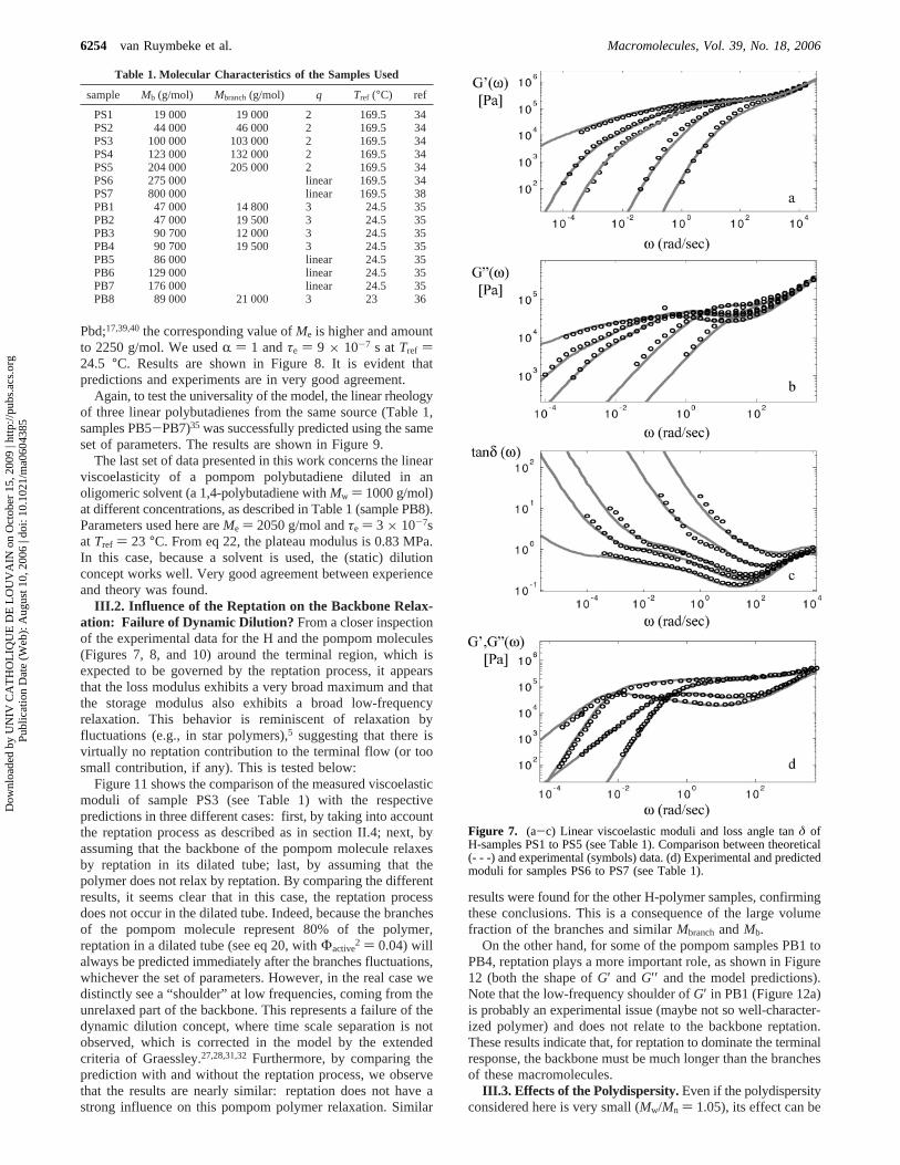
III.1. Parameters and Predictions. H-Polystyrene Melts.To assess the model in more detail, we compared predictionswith available experimental relaxation moduli from differentsets of polymers (H or pompom). The first set is composed ofseveral polystyrene H-polymers synthesized and measured byRoovers.34 Their average molecular weights are listed in Table1 (samples PS1-PS5).34-36,38

Backbone and branches of these samples have the samemolecular weight. The model has two parameters that need tobe defined: the entanglement molecular weight,Me, and theRouse time of a segmentτe. We used consistentlyτe ) 8 ×10-4 s, Me ) 16 000 g/mol (atTref ) 169.5°C). The value ofthe plateau modulus,GN

0, was 2.3× 105 Pa. Given that thedensity of the PS is 0.959 kg/m3, this value is consistentwith7,17,39,40 GN

0) (4/5)(FRT/Me) within 15%. Such a smalldeviation is acceptable and in line with what has been reportedin the literature when using similar modeling efforts to predictpolymer rheology.41 The origin of this small deviation remainsa puzzle at present, but two issues that should be consideredare the small experimental uncertainties in the high-frequencyrheometrical measurements and the fact that the couplingbetween the faster Rouse relaxation of an entanglement segmentand the branches relaxation (which can start before the formerrelaxes fully) are not taken into account. Furthermore, we fixedthe value of the dilution exponentR to 1.42 We decided to keepR constant for all the polymers analyzed in this work in orderto test the predictive capability of the model without having anadditional parameter. Since there is no real consensus on thevalue of this exponent, we fixed its value to 1 as proposed inrefs 13, 14, 17, 18, and 24. Results obtained with this set ofparameters are shown in Figure 7. Very good agreement betweenexperimental data and the model predictions was found for allsamples without any adjustable parameters. This is already adeparture from the earlier approaches which used a sensitiveadjustable parameter,p2. To ensure the universal validity of themodel, we also tested two linear PS samples, again synthesizedand measured by Roovers and co-workers,34,38 at the same

temperature (see Table 1, samples PS6 and PS7). Comparisonbetween model predictions and experimental data are shown inFigure 7d, with the same set of parameters. Note that a linearpolymer is a limiting case of this model, i.e., an H-moleculewith branches of zero length.

Pompom Polybutadiene Melts and Solutions.The particularmolecules have three branches on each side of the backbone (q) 3) and are described in Table 1 (see samples PB1-PB4).35

The rheological properties were measured at 24.5°C.33 Becausethey contain a large fraction of 1,2-microstructure (about 50%),the value of their plateau modulus (GN

0 ) 700 000 Pa) wasfound low compared to the typical value of 1 MPa for 1,4-

Figure 5. Normalized Wesslau molecular weight distribution. Theoverall distribution is divided to five equivalent surfaces (separated bythe black continuous lines). Each of the surfaces is represented by itsaverage molecular weight (- - -).

Figure 6. Model predictions of the relaxation moduli of samples PB4(see Table 1) for different values of polydispersity: 1, 1.05, 1.1, and1.2 (from black to light gray). Polydispersity is considered (a) for thebackbone molecular weight only; (b) for the branch molecular weightonly; (c and d) for both the backbone and the branch molecular weights.

Macromolecules, Vol. 39, No. 18, 2006 Linear Rheology of Branched Polymers6253

Dow

nloa

ded

by U

NIV

CA

TH

OL

IQU

E D

E L

OU

VA

IN o

n O

ctob

er 1

5, 2

009

| http

://pu

bs.a

cs.o

rg

Pub

licat

ion

Dat

e (W

eb):

Aug

ust 1

0, 2

006

| doi

: 10.

1021

/ma0

6043

85

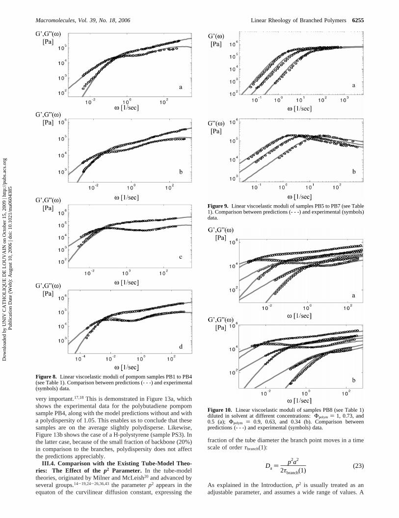
Pbd;17,39,40the corresponding value ofMe is higher and amountto 2250 g/mol. We usedR ) 1 andτe ) 9 × 10-7 s atTref )24.5 °C. Results are shown in Figure 8. It is evident thatpredictions and experiments are in very good agreement.

Again, to test the universality of the model, the linear rheologyof three linear polybutadienes from the same source (Table 1,samples PB5-PB7)35 was successfully predicted using the sameset of parameters. The results are shown in Figure 9.

The last set of data presented in this work concerns the linearviscoelasticity of a pompom polybutadiene diluted in anoligomeric solvent (a 1,4-polybutadiene withMw ) 1000 g/mol)at different concentrations, as described in Table 1 (sample PB8).Parameters used here areMe ) 2050 g/mol andτe ) 3 × 10-7sat Tref ) 23 °C. From eq 22, the plateau modulus is 0.83 MPa.In this case, because a solvent is used, the (static) dilutionconcept works well. Very good agreement between experienceand theory was found.

III.2. Influence of the Reptation on the Backbone Relax-ation: Failure of Dynamic Dilution? From a closer inspectionof the experimental data for the H and the pompom molecules(Figures 7, 8, and 10) around the terminal region, which isexpected to be governed by the reptation process, it appearsthat the loss modulus exhibits a very broad maximum and thatthe storage modulus also exhibits a broad low-frequencyrelaxation. This behavior is reminiscent of relaxation byfluctuations (e.g., in star polymers),5 suggesting that there isvirtually no reptation contribution to the terminal flow (or toosmall contribution, if any). This is tested below:

Figure 11 shows the comparison of the measured viscoelasticmoduli of sample PS3 (see Table 1) with the respectivepredictions in three different cases: first, by taking into accountthe reptation process as described as in section II.4; next, byassuming that the backbone of the pompom molecule relaxesby reptation in its dilated tube; last, by assuming that thepolymer does not relax by reptation. By comparing the differentresults, it seems clear that in this case, the reptation processdoes not occur in the dilated tube. Indeed, because the branchesof the pompom molecule represent 80% of the polymer,reptation in a dilated tube (see eq 20, withΦactive

2 ) 0.04) willalways be predicted immediately after the branches fluctuations,whichever the set of parameters. However, in the real case wedistinctly see a “shoulder” at low frequencies, coming from theunrelaxed part of the backbone. This represents a failure of thedynamic dilution concept, where time scale separation is notobserved, which is corrected in the model by the extendedcriteria of Graessley.27,28,31,32Furthermore, by comparing theprediction with and without the reptation process, we observethat the results are nearly similar: reptation does not have astrong influence on this pompom polymer relaxation. Similar

results were found for the other H-polymer samples, confirmingthese conclusions. This is a consequence of the large volumefraction of the branches and similarMbranchandMb.

On the other hand, for some of the pompom samples PB1 toPB4, reptation plays a more important role, as shown in Figure12 (both the shape ofG′ and G′′ and the model predictions).Note that the low-frequency shoulder ofG′ in PB1 (Figure 12a)is probably an experimental issue (maybe not so well-character-ized polymer) and does not relate to the backbone reptation.These results indicate that, for reptation to dominate the terminalresponse, the backbone must be much longer than the branchesof these macromolecules.

III.3. Effects of the Polydispersity.Even if the polydispersityconsidered here is very small (Mw/Mn ) 1.05), its effect can be

Table 1. Molecular Characteristics of the Samples Used

sample Mb (g/mol) Mbranch(g/mol) q Tref (°C) ref

PS1 19 000 19 000 2 169.5 34PS2 44 000 46 000 2 169.5 34PS3 100 000 103 000 2 169.5 34PS4 123 000 132 000 2 169.5 34PS5 204 000 205 000 2 169.5 34PS6 275 000 linear 169.5 34PS7 800 000 linear 169.5 38PB1 47 000 14 800 3 24.5 35PB2 47 000 19 500 3 24.5 35PB3 90 700 12 000 3 24.5 35PB4 90 700 19 500 3 24.5 35PB5 86 000 linear 24.5 35PB6 129 000 linear 24.5 35PB7 176 000 linear 24.5 35PB8 89 000 21 000 3 23 36

Figure 7. (a-c) Linear viscoelastic moduli and loss angle tanδ ofH-samples PS1 to PS5 (see Table 1). Comparison between theoretical(- - -) and experimental (symbols) data. (d) Experimental and predictedmoduli for samples PS6 to PS7 (see Table 1).

6254 van Ruymbeke et al. Macromolecules, Vol. 39, No. 18, 2006

Dow

nloa

ded

by U

NIV

CA

TH

OL

IQU

E D

E L

OU

VA

IN o

n O

ctob

er 1

5, 2

009

| http

://pu

bs.a

cs.o

rg

Pub

licat

ion

Dat

e (W

eb):

Aug

ust 1

0, 2

006

| doi

: 10.

1021

/ma0

6043

85

very important.17,18 This is demonstrated in Figure 13a, whichshows the experimental data for the polybutadiene pompomsample PB4, along with the model predictions without and witha polydispersity of 1.05. This enables us to conclude that thesesamples are on the average slightly polydisperse. Likewise,Figure 13b shows the case of a H-polystyrene (sample PS3). Inthe latter case, because of the small fraction of backbone (20%)in comparison to the branches, polydispersity does not affectthe predictions appreciably.

III.4. Comparison with the Existing Tube-Model Theo-ries: The Effect of the p2 Parameter. In the tube-modeltheories, originated by Milner and McLeish20 and advanced byseveral groups.14-19,24-26,36,43 the parameterp2 appears in theequaton of the curvilinear diffusion constant, expressing the

fraction of the tube diameter the branch point moves in a timescale of orderτbranch(1):

As explained in the Introduction,p2 is usually treated as anadjustable parameter, and assumes a wide range of values. A

Figure 8. Linear viscoelastic moduli of pompom samples PB1 to PB4(see Table 1). Comparison between predictions (- - -) and experimental(symbols) data.

Figure 9. Linear viscoelastic moduli of samples PB5 to PB7 (see Table1). Comparison between predictions (- - -) and experimental (symbols)data.

Figure 10. Linear viscoelastic moduli of samples PB8 (see Table 1)diluted in solvent at different concentrations:Φpolym ) 1, 0.73, and0.5 (a); Φpolym ) 0.9, 0.63, and 0.34 (b). Comparison betweenpredictions (- - -) and experimental (symbols) data.

Da ) p2a2

2τbranch(1)(23)

Macromolecules, Vol. 39, No. 18, 2006 Linear Rheology of Branched Polymers6255

Dow

nloa

ded

by U

NIV

CA

TH

OL

IQU

E D

E L

OU

VA

IN o

n O

ctob

er 1

5, 2

009

| http

://pu

bs.a

cs.o

rg

Pub

licat

ion

Dat

e (W

eb):

Aug

ust 1

0, 2

006

| doi

: 10.

1021

/ma0

6043

85

valuep2 < 1, typically used in most branched polymer studies,implies a slowing- down of the backbone relaxation.14-19,24-26,36,43

There are also situations where a value of 1 is used.14,24,25Ingeneral, this parameter is considered to depend on chemistryonly,14-19 although there are suggestions of possible dependenceon the macromolecular architecture as well.24-26 In the presentwork, we fix p2 ) 1 and there is no need to vary the value ofp2 across the different samples. This represents a distinctdifference that needs being elaborated. Thus, we briefly discussbelow the differences in the calculations of the differentcontributing relaxation processes.

The reptation time of the backbone is given by eqs 19 and20. Considering that reptation takes place in a (nearly) undi-luted tube, this already slows down the backbone relax-ation process. However, as shown in the literature, thismodification is not enough.24,27-30 The main contribution to theslower backbone relaxation, and key difference between thecurrent approach and the previous ones14,15,17,18,24,25,36-43 origi-nates from the factor (1- xd), which is used in the equation ofthe reptation time;xd represents the deeper inner backbonesegments relaxed by fluctuations before the reptation process.As already explained in section II.4, to analyze the backbonerelaxation by reptation, we consider that the backbone center-of-mass diffuses along its total average equilibrium length.Indeed, even if some segments are already relaxed by fluctua-tions, they still have a nonzero equilibrium length that weconsider here. In fact, the same conclusion was already drawnfrom the original time-marching model applied to highlyasymmetric stars.27 Last, the respective difference observed inthe calculation of the backbone fluctuations times, whichprecedes and slows down the backbone reptation process arisesprincipally from the rescaling of the variablexb, from the outerfree end of a branch to the middle of the molecule (see sectionsII.1 and II.3).

IV. Conclusions

We have developed a general coarse-grained model forpredicting the linear viscoelasic properties of branched polymersfrom the knowledge of their molecular structure and threeviscoelastic parameters, i.e., the Rouse time of an entanglementsegment, the plateau modulus and the entanglement molecularweight. This is an extension of earlier work using a time-marching algorithm to successfully predict the rheology of linearand star polymers. uses the physics of tube-based theories,originated by McLeish and co-workers. We have appropriatelymodified and extended this earlier model by proposing a newmacromolecular coordinate system and accounting for thediffusion of the branching points and the polydispersity, withinthe framework of dynamic tube dilation (using the citeria ofGraessley). We have obtained excellent predictions for the linearviscoelastic properties of different complex macromoleculararchitectures, such as H polymers and pompom polymers,without any adjustable parameters. It has been demonstratedthat polydispersity is very important, even when it amounts to5% only. There are still some issues at stake, such as the valueof the dilution exponent, the validity of the rubber elasticityrelation within 15%, and the coupling of the different relaxationmodes. Nevertheless, the successful and self-consistent applica-tion of the model to different chemistries and architectures givesus confidence that the proposed methodology represents a

Figure 11. Storage and loss moduli (a) and tanδ (b) of sample PS3calculated without reptation (light gray), by considering the “solvent”polymer fraction described by eqs 19 and 20 (dark gray) or byconsidering the unrelaxed fraction of the sample equal to the volumetricfraction of the (inner) backbone (black).

Figure 12. Storage and loss moduli of samples PB1 (a), PB2 (b), andPB4 (c), calculated without any reptation (×××), or with reptation,by considering that the “solvent” polymer fraction for the backbone isdescribed by eqs 19 and 20 (- - -); see text for details.

6256 van Ruymbeke et al. Macromolecules, Vol. 39, No. 18, 2006

Dow

nloa

ded

by U

NIV

CA

TH

OL

IQU

E D

E L

OU

VA

IN o

n O

ctob

er 1

5, 2

009

| http

://pu

bs.a

cs.o

rg

Pub

licat

ion

Dat

e (W

eb):

Aug

ust 1

0, 2

006

| doi

: 10.

1021

/ma0

6043

85

powerful generic approach for predicting the linear rheologyof branched polymers.

Acknowledgment. Helpful discussions with M. Kapnistosare gratefully acknowledged. This work has been supported bythe EU (NoE-Softcomp, Grant NMP3-CT-2004-502235; Indi-vidual Marie Curie fellowship- DYCOSYS to E.v.R., GrantMEF-CT-2005-024298).

Appendix I: Relaxation Modulus of a Pompom Molecule

The relaxation modulus of a monodisperse polymer melt ora concentrated solution is described in general by three terms:the first represents the relaxation of the polymer from itsequilibrium state (by reptation, fluctuations, or constraintrelease), the second is longitudinal modes relaxation, and thethird is fast Rouse motion inside the tube:4,7,44

The relaxation modulusF(t) of the polymer is calculated bysumming up all contributions from segments along the branchesand the backbone:

A given segment will contribute to the modulus if it has notbeen relaxed by any of the three possible relaxation mecha-nisms: prept, pfluc, andpenvir represent the probabilities that thesegment x remains oriented by reptation, fluctuations orconstraint release, respectively. These terms are described insections II.3, II.4 and II.5. Because the reptation and thefluctuations times of a segment are not necessary time-independent (for example they may decrease with increasing

the polymer fraction acting as a solvent), we use a time-marching algorithm,27 which determines the survival prob-abilities of each segment at a given timetk from the corre-sponding values at the previous timetk-1:

The survival probability attk is the product of the survival prob-ability at tk-1 and the survival probability during the time intervaltaken betweentk-1 andtk. The latter probabilities are calculatedfrom the values of the relaxation timesτrelax(xi,tk) calculated attime tk, after the update ofΦ(tk), the polymer fraction acting asa solvent in the reptation and fluctuation processes:

The time τrelax represents either the reptation time or thefluctuations time of the segmentxi. The second and third terms,calculated as in ref 7, are functions of the Rouse time of thebackbone and of the branches

whereZ is the number of entanglements andN, the number ofKhun segments, and

Me is the entanglement molecular weight andτe is its Rousetime of an entanglement segment:

where ú0 represents the monomeric friction coefficient. Thestorage and loss moduli are then calculated from the relaxationmodulusG(t) by using the Schwarzl relations, which are anapproximation of the Fourier transform.6,45

Appendix II: Branches Fluctuations

The branches of a pompom molecule relax exactly as thearms of a star molecule. As described by Milner and McLeish,20

each branch has an equilibrium length,Leq(Mbranch), coming fromthe balance between an entropic force which tends to reducethe distance between the end chain and the branching point,and a topological force, representing the effect of the environ-ment, which prevents this retraction. Because the real length ofthe branch fluctuates about this equilibrium length (which isthe most probable), the initial tube segments relax little by little,from the outer to the inner one. Their corresponding fluctuations

Figure 13. Storage and loss moduli of samples PB4 (a) and PS3 (b),calculated by considering a polydispersity of 1.05 (- - -), or byconsidering the samples as monodisperse (×××).

G(t) )

GN0F(t) + 1

4GN

0FRouse,longitudinal(t) + 54

GN0Ffast Rouse(t) (I-1)

F(t) ) æb∫0

1(prept(xb,t)pfluc(xb,t)penvir(xb,t)) dxb +

æbranch∫0

1(pfluc(xbranch,t)penvir(xbranch,t)) dxbranch (I-2)

pfluc(xi,tk) ) pfluc(xi,tk-1)pfluc(xi,[tk-1,tk]) (I-3)

prept(xi,tk) ) prept(xi,tk-1)prept(xi,[tk-1,tk]) (I-4)

psurvival(xi,[tk-1,tk]) ) exp( -(∆t)

τrelax(xi,tk,Φ(tk))) (I-5)

FRouse,longitudinal) (1

Zæb ∑

j)1

Z-1

exp(-j2t

τRouse(Mb + 2Mbranch)) +

1

Zæbranch∑

j)1

Z-1

exp(-j2t

τRouse(Mbranch))) (I-6)

Ffast Rouse) (1

Zæb ∑

j)Z

N

exp(-2j2t

τRouse(Mb + 2Mbranch)) +

1

Zæbranch∑

j)Z

N

exp(-2j2t

τRouse(Mbranch))) (I-7)

τRouse,Mi) τe(Mi

Me)2

, i ) branch,b (I-8)

τe )ú0b

2

3π2kT(Me

m0)2

(I-9)

Macromolecules, Vol. 39, No. 18, 2006 Linear Rheology of Branched Polymers6257

Dow

nloa

ded

by U

NIV

CA

TH

OL

IQU

E D

E L

OU

VA

IN o

n O

ctob

er 1

5, 2

009

| http

://pu

bs.a

cs.o

rg

Pub

licat

ion

Dat

e (W

eb):

Aug

ust 1

0, 2

006

| doi

: 10.

1021

/ma0

6043

85

time increases exponentially with the depth of the segment:

Since the fluctuations times of the segments are exponentiallydependent on their location on the branch, we consider that theexternal segments already relaxed act as a solvent for therelaxation of the inner segments. This is the idea of dynamicdilution:22,23 if a fraction (1- Φ(tk,xbranch)) of the polymer actsas a solvent, the molecular weight between two effectiveentanglements (which have an effective role in the orientationof the polymer),Me(tk,xbranch), increases

where Me,0 is the nominal entanglement molecular weight(before dilution) and the parameterR is the dilution exponent,usually between 1 and 4/3.42,46This effect must be included inthe expression II-2:

The functionΦ(tk,xbranch) represents the unrelaxed part of thepompom polymer, when the branches are relaxed until thesegment defined by the normalized variablexbranch, at time tk.In this particular case, because the reptation process occurs onlyafter the relaxation of the branches has been completed, no“dynamic reptation solvent” is taken into account inΦ(tk,xbranch).Therefore, this variable does not depend on the time:

In this expression, the value ofxb, which is defined as in Figure1, is directly calculated fromxbranch:

As introduced in ref 20, for segments having a potentialU(xa)< kT, their early fluctuations times do not follow eq II.4 butare described by a Rouse process:

where τR,branch is the Rouse time of the branch. No polymersolvent is considered in this equation. Indeed, to act as a solvent,the relaxed part of the polymer must be well-separated in timescale from the relaxing segments. This is not observed herebecause of the speed of the Rouse relaxation.

The transition between the two fluctuation processes happensat a transition segmentxtrans, for which the potentialU(xtrans) )kT, and it is described as

By using these expressions, we do not need to calculate anywaiting time τ0, contrary to the other approaches in theliterature.20

References and Notes

(1) de Gennes, P. G.J. Chem. Phys.1971, 55, 527.(2) Doi, M.; Edwards, S. F.The Theory of Polymer Dynamics; Oxford

University Press: New York, 1986.(3) Watanabe, H.Prog. Polym. Sci.1999, 24, 1253.(4) Marrucci, G.; Greco, F.; Ianniruberto, G.Curr. Opin. Colloid Interface

Sci. 1999, 4, 283. Evaraers, R.; Sukumaran, S. K.; Grest, G. S.;Svaneborg, C.; Sivasubramanian, A.; Kremer, K.Science2004, 303,823. Likhtman, A. E.Macromolecules2005, 38, 6128.

(5) McLeish, T. C. B.AdV. Phys.2002, 51, 1379.(6) van Ruymbeke, E.; Keunings, R.; Stephenne, V.; Hagenaars, A.; Bailly,

C. Macromolecules2002, 35, 2689.(7) Likhtman, A. E.; McLeish, T.Macromolecules2002, 35, 6332.(8) Hsieh, H. L.; Quirk, R. P.Anionic Polymerization: Principles and

Practical Applications; Marcel Dekker: New York, 1996.(9) Pitsikalis, M.; Pispas, S.; Mays, J. W.; Hadjichristidis, N.AdV. Polym.

Sci.1998, 135, 1.(10) Hadjichristidis, N.; Pitsikalis, M.; Pispas, S.; Iatrou, H.; Vlahos, C.

AdV. Polym. Sci.1999, 142, 71.(11) Roovers, J.; Graessley, W. W.Macromolecules1981, 14, 766. Roovers,

J.Polymer1979, 20, 843. Roovers, J.; Toporowski, P.Macromolecules1987, 20, 2300.

(12) Knauss, D. M.; Al-Muallem, H. A.; Huang, T.; Wu, D. T.Macro-molecules2000, 33, 3557.

(13) Larson, R. G.Macromolecules2001, 34, 4556.(14) McLeish, T. C. B.; Allgaier, J.; Bick, D. K.; Bishko, G.; Biswas, P.;

Blackwell, R.; Blottiere, B.; Clarke, N.; Gibbs, B.; Groves, D. J.;Hakiki, A.; Heenan, R. K.; Johnson, J. M.; Kant, R.; Read, D. J.;Young, R. N.Macromolecules1999, 32, 6734.

(15) Daniels, D. R.; McLeish, T. C. B.; Crosby, B. J.; Young, R. N.;Fernyhough, C. M.Macromolecules2001, 34, 7025.

(16) Blackwell, R. J.; Harlen, O. G.; McLeish, T. C. B.Macromolecules2001, 34, 2579.

(17) Kapnistos, M.; Vlassopoulos, D.; Roovers, J.; Leal, L. G.Macromol-ecules2005, 38, 7852.

(18) Kapnistos, M.; Koutalas, G.; Hadjichristidis, N.; Roovers, J.; Lohse,D. J.; Vlassopoulos, D.Rheol. Acta, submitted, 2006.

(19) McLeish, T. C. B.; Larson, R. G.J. Rheol.1998, 42, 81.(20) Milner, S. T.; McLeish, T. C. B.Macromolecules1997, 30, 2159.(21) Milner, S. T.; McLeish, T. C. B.Macromolecules1998, 31, 7479.(22) Marrucci, G.J. Polym. Sci., Polym. Phys. Ed.1985, 23, 159.(23) Ball, R. C.; McLeish, T. C. B.Macromolecules1989, 22, 1911.

McLeish, T. C. B.J. Rheol.2003, 47, 177.(24) Frischknecht, A. L.; Milner, S. T.; Pryke, A.; Young, R. N.; Hawkins,

R.; McLeish, T. C. B.Macromolecules2002, 35, 4801.(25) Lee, J. H.; Fetters, L. J.; Archer, L. A. Macromolecules2005, 38,

4484.(26) Lee, J. H.; Fetters, L. J.; Archer, L. A.Macromolecules2005, 38,

10763.(27) van Ruymbeke, E.; Keunings, R.; Bailly, C.J. Non-Newtonian Fluid

Mech.2005, 128, 7.(28) Struglinski, M. J.; Graessley, W. W.Macromolecules1985, 18, 2630.(29) Tsenoglou, C.ACS Polym. Prepr.1987, 28, 185. Tsenoglou, C.

Macromolecules1991, 24, 1762.(30) des Cloizeaux, J.J. Europhys. Lett.1988, 5, 437.(31) Watanabe, H.; Ishida, S.; Matsumiya, Y.; Inoue, T.Macromolecules

2004, 37, 1937.(32) Watanabe, H.; Ishida, S.; Matsumiya, Y.; Inoue, T.Macromolecules

2004, 37, 6619. Watanabe, H.; Matsumiya, Y.; Inoue, T.Macromol-ecules2002, 35, 2339.

(33) Park, S. J.; Larson, R. G.Macromolecules2004, 37, 597.(34) Roovers, J.Macromolecules1984, 17, 1196.(35) Archer, L. A.; Varshney, S. K.Macromolecules1998, 31, 6348.(36) Juliani; Archer, L. A.Macromolecules2002, 35, 10048. Archer, L.

A.; Juliani Macromolecules2004, 37, 1076.(37) Wesslau, H.Makrom Chemie1956, 20, 111.(38) Graessley, W. W.; Roovers, J.Macromolecules1979, 12, 959.

U(xbranch) ) 3kT

2Nb2(Leqxbranch)

2 + const (II-1)

ln τlate(xbranch) )U(xbranch)

kT+ const (II-2)

Me(t,xbranch) )Me,0

Φ(tk,xbranch)R (II-3)

∂ ln τlate(xbranch)

∂xbranch) 3( Mbranch

Me(tk,xbranch))xbranch (II-4)

Φ(tk,xbranch) ) Φ(xbranch) ) æb(1 - xb) + æbranch(1 - xbranch)(II-5)

xb )xbranchMbranch

Mbranch+ Mb/2(II-6)

τearly(xbranch) ) 9π3

16(Mbranch

Me,0)2

τR,branchxbranch4 (II-7)

τfluc(xbranch) ) τearly(xbranch) for xbranch< xtrans (II-8)

τfluc(xbranch) ) τearly(xtrans) exp(∆U(xtransf xbranch)

kT )for xbranch> xtrans (II-9)

6258 van Ruymbeke et al. Macromolecules, Vol. 39, No. 18, 2006

Dow

nloa

ded

by U

NIV

CA

TH

OL

IQU

E D

E L

OU

VA

IN o

n O

ctob

er 1

5, 2

009

| http

://pu

bs.a

cs.o

rg

Pub

licat

ion

Dat

e (W

eb):

Aug

ust 1

0, 2

006

| doi

: 10.

1021

/ma0

6043

85

(39) Larson, R. G.; Sridhar, T.; Leal, L. G.; McKinley, G. H.; Likhtman,A. E.; McLeish, T. C. B.J. Rheol.2003, 47, 809. Fetters, L. J.; Lohse,D. J.; Richter, D.; Witten, T. A.; Zirkel, A.Macromolecules1994,27, 4639.

(40) Ferry, J. D.Viscoelastic Properties of Polymers, 3rd ed.; Wiley: NewYork, 1980.

(41) Liu, C. Y.; He, J.; Keunings, R.; Bailly, C. Do tube models yieldconsistent predictions for the relaxation time and apparent plateaumodulus of entangled linear polymers?Macromolecules2006, in press.

(42) Rubinstein, M.; Colby, R. H.Polymer Physics; Oxford UniversityPress: New York, 2003. Colby, R. H.; Rubinstein, M.Macromolecules1990, 23, 2753.

(43) Frischknecht, A. L.; Milner, S. T.Macromolecules2000, 33, 9764.(44) Miros, A.; Vlassopoulos, D.; Likthman, A. E.; Roovers, J.J. Rheol.

2003, 47, 163.(45) Schwarzl, F. R.Rheol. Acta1971, 10, 166.(46) Raju, V. R.; Menezes, E. V.; Marin. G.; Graessley, W. W.Macro-

molecules1981, 14, 1668. Daniels, D. R.; McLeish, T. C. B.; Kant,R.; Crosby, B. J.; Young, R. N.; Pryke, A.; Allgaier, J.; Groves, D.J.; Hawkins, R. J.Rheol. Acta2001, 40, 403. Tao, H.; Huang, C.;Lodge, T. P.Macromolecules1999, 32, 1212. Park, S. J.; Larson, R.G. J. Rheol.2003, 47, 199.

MA0604385

Macromolecules, Vol. 39, No. 18, 2006 Linear Rheology of Branched Polymers6259

Dow

nloa

ded

by U

NIV

CA

TH

OL

IQU

E D

E L

OU

VA

IN o

n O

ctob

er 1

5, 2

009

| http

://pu

bs.a

cs.o

rg

Pub

licat

ion

Dat

e (W

eb):

Aug

ust 1

0, 2

006

| doi

: 10.

1021

/ma0

6043

85