NBER WORKING PAPER SERIES

A GENERAL RATIONALE FOR A GOVERNMENTAL ROLE IN THE RELIEFOF LARGE RISKS

Steven Shavell

Working Paper 20192http://www.nber.org/papers/w20192

NATIONAL BUREAU OF ECONOMIC RESEARCH1050 Massachusetts Avenue

Cambridge, MA 02138June 2014

I thank Peter Diamond, Georges Dionne, Kenneth Froot, Louis Kaplow, and A. Mitchell Polinskyfor comments, Michael Belinsky and Jonathan Borowsky for research assistance, and the John M.Olin Center for Law, Economics, and Business at Harvard University for research support. The viewsexpressed herein are those of the author and do not necessarily reflect the views of the National Bureauof Economic Research.

NBER working papers are circulated for discussion and comment purposes. They have not been peer-reviewed or been subject to the review by the NBER Board of Directors that accompanies officialNBER publications.

© 2014 by Steven Shavell. All rights reserved. Short sections of text, not to exceed two paragraphs,may be quoted without explicit permission provided that full credit, including © notice, is given tothe source.

A General Rationale for a Governmental Role in the Relief of Large RisksSteven ShavellNBER Working Paper No. 20192June 2014JEL No. D6,D8,K2

ABSTRACT

The government often provides relief against large risks, such as disasters. A simple, general rationalefor this role of government is considered here that applies even when private contracting to share risksis not subject to market imperfections. Specifically, the optimal private sharing of risks will not resultin complete coverage against them when they are sufficiently large. Hence, when such risks eventuate,the marginal utility to individuals of governmental relief may exceed the marginal value of publicgoods. Consequently, social welfare may be raised if the government reduces public goods expendituresand directs these freed resources toward individuals who have suffered losses.

Steven ShavellHarvard Law School1575 Massachusetts AvenueHauser Hall 508Cambridge, MA 02138and NBERshavell@law.harvard.edu

An online appendix is available at:http://www.nber.org/data-appendix/w20192

1

A General Rationale for a Governmental Role in the Relief of Large Risks

Steven Shavell*

Forthcoming in the Journal of Risk and Uncertainty JEL classifications: D6, D8, K2

The government often provides relief against large risks, such as disasters.

A simple, general rationale for this role of government is considered here that

applies even when private contracting to share risks is not subject to market

imperfections. Specifically, the optimal private sharing of risks will not result in

complete coverage against them when they are sufficiently large. Hence, when

such risks eventuate, the marginal utility to individuals of governmental relief

may exceed the marginal value of public goods. Consequently, social welfare

may be raised if the government reduces public goods expenditures and directs

these freed resources toward individuals who have suffered losses.

1. Introduction

The government plays a well-recognized role in providing relief against

many large risks. Notably, the government traditionally furnishes disaster

assistance and subsidizes markets for flood and earthquake insurance.1

That the government is often observed to ameliorate substantial risks

naturally raises the question about the justification for that policy. I consider here

a general rationale for the government to relieve significant risks that applies even

* Samuel R. Rosenthal Professor of Law and Economics, Harvard Law School, and

Research Associate, National Bureau of Economic Research. I thank Peter Diamond, Georges Dionne, Kenneth Froot, Louis Kaplow, and A. Mitchell Polinsky for comments, Michael Belinsky and Jonathan Borowsky for research assistance, and the John M. Olin Center for Law, Economics, and Business at Harvard University for research support.

1 On the role of the government in disaster assistance, see generally the historical account of Moss (1999) and, for example, the website of the Federal Emergency Management Agency (FEMA), www.fema.gov; on government programs to foster flood and earthquake insurance, see FEMA (2002) and the website of the California Earthquake Authority, www.earthquakeauthority.com. The government also promotes and furnishes other types of insurance, such as disability and health insurance, of course, but the basis for these types of aid appears to be different from that discussed here.

2

when, as I will assume, private contracting to share risks is perfect (unimpeded by

transaction costs, asymmetric information, externalities, or other sources of

market failure). The rationale, in essence, is that the optimal private sharing of

very large risks will not result in complete coverage against them. Therefore,

when the risks eventuate, the marginal utility to individuals of relief from the

government will be high in a relative sense and may exceed the marginal value to

individuals of public goods. Consequently, social welfare may be raised if the

government reduces public goods expenditures and directs these freed resources

toward individuals who have suffered losses.

Although the foregoing argument is straightforward, it does not seem to

have been clearly articulated before. I develop it below employing a simple

model involving a population of identical individuals, a single consumption good,

a risk of loss of the consumption good—where this accident risk may be

correlated across individuals—frictionless joint contracting among all individuals

to share risk, and a government that produces a public good.

Two times are considered in the model: time 1, before risk resolves itself,

and time 2, after possible accident losses have occurred. At time 1, individuals

pay a tax to finance the public good and they contract in a privately-optimal way

to share risk. Their best risk-sharing contracts do not lead to full coverage against

loss. Indeed, in the extreme case of a single, economy-wide risk (a flood that

affects everyone), contracting would not result in any coverage; the

privately-optimal risk-sharing contract would be the null contract.

The main results shown are these. First, there exists a welfare-enhancing

policy under which the government grants relief to accident victims whenever the

number of accidents in the population is sufficiently high.2

2 The policy of government relief will, however, result in some crowding out of payments

made to accident victims under private risk-sharing contracts.

Welfare is enhanced

3

for the reason I noted above: when the number of accidents is high, the wealth of

accident victims after optimal risk-sharing is relatively low and their marginal

utility of income is relatively high, implying that they will be made better off if

resources are shifted from public goods to them by the making of relief payments.

Second, a policy of government relief exists that achieves the first-best outcome

in terms of both risk-sharing and provision of public goods. Third, a policy of

government subsidy of risk-sharing contracts (analogous to the subsidy of

insurance contracts) may provide social benefits similar to those of government

relief.3

The general justification for government aid in the event of large risks that

is examined in the model seems consistent with actual policy in at least an

approximate sense. On one hand, the important risks mentioned above that the

government helps to alleviate have the character that they may affect many

individuals simultaneously; this is frequently true of disasters. On the other hand,

private insurance coverage against these positively correlated risks tends to be

circumscribed,

And fourth, a policy under which taxes are lowered appropriately as the

number of accidents increases allows the first-best outcome to be achieved

without government relief or the subsidy of risk-sharing contracts.

4

The rationale for government help in the face of large, correlated risks

presented here is different from those discussed in prior writing to my

making it plausible that a shift of resources from the provision of

public goods to those who have suffered losses would often be socially desirable.

3 As will be seen, a well-designed ex post subsidy of coverage payments made to accident

victims will be socially beneficial, but an ex ante subsidy of risk-sharing contracts cannot improve social welfare because it does not make public goods expenditures depend on the occurrence of accidents.

4 Regarding the paucity (and high cost) of private insurance coverage against catastrophic

events, see generally Froot (1999, 2001), and also, for example, Jaffee and Russell (1997) and Cummins (2006). As Froot emphasizes, the scarcity of coverage due to these correlated losses is significant, even though one might have expected otherwise, given the existence of the reinsurance industry and the size of global capital markets.

4

knowledge. First, some authors who have stressed that insurance coverage

against disasters is limited suggest that this problem per se justifies government

relief.5 But that conclusion does not follow when the limited coverage is the

result of privately-optimal risk sharing—government relief is warranted only if

the government provides public goods. If the government has no need to provide

public goods, the government will not have command over resources to

advantageously draw upon to furnish relief when privately-optimal risk sharing

leaves individuals wanting.6

A second reason for government aid is premised on the assumption that

the government is uniquely able to distribute risk over the entire population

through the medium of the income tax system. Under this assumption, when the

government assumes a risk, like that of a natural disaster, the impact on the

individual taxpayer in a large population is small, making the government a

desirable bearer of risk.

7

The foregoing argument is different from the one I

consider because I assume that all individuals in the population are able to jointly

contract to share risk. Hence, in the model examined below, the government does

not enjoy any advantage over the private sector in the spreading of private risks

across the population.

5 See, for example, the discussion of the coverage of terrorism risk in Cummins (2006), p. 375.

6 The reader can verify that if there is no demand for public goods, the first-best outcome described in Proposition 1 is achieved under privately optimal risk-sharing described in Proposition 2.

7 This argument is developed by Arrow and Lind (1970), who show under certain assumptions not only that the risk-bearing cost per individual tends to zero with the population size, but also that the aggregate risk-bearing cost tends to zero.

5

A third justification for government relief is that individuals may

systematically underestimate risk, leading them to underinsure.8 A fourth

justification is adverse selection, for it can reduce or eliminate private coverage

even though coverage would be socially desirable.9

Finally, let me comment on writing that is skeptical of the basis for a

governmental role in relieving large risks. The most commonly made argument

against a governmental role is an expression of the general view that

governmental intervention in reasonably well-functioning markets—here

insurance markets—tends to be undesirable.

These two reasons for

government aid are obviously different from that advanced here.

10

More particular arguments are also made against government relief against

risk. One of note is that although problems of moral hazard (for example, an

insured person inefficiently building a house in an area vulnerable to floods) may

lead to limited coverage against risk, moral hazard is not a justification for

government relief. Moral hazard is in fact generally exacerbated by provision of

government relief.

This classic laissez-faire belief,

though, is not necessarily valid when applied to insurance markets. As I have

emphasized is the case in the model developed here, even if private markets for

risk-sharing function efficiently, the government should sometimes act to relieve

risk using funds that otherwise would finance public goods.

11

8 See, for example, Kunreuther, et al (1978).

Such problems are serious ones that should clearly be taken

into account in the design of policies for relief, but the model here abstracts from

them.

9 See, for example, Dionne, Doherty, and Fombaron (2000) for a survey on adverse

selection in insurance markets. 10 See, for example, Priest (1999); and see Cummins (2006), who also emphasizes the

point that government coverage can supplant private coverage. 11 See Kaplow (1991).

6

2. The Model

2.1 Basic assumptions. There is an economy of n individuals with

identical utility functions. Each individual derives utility from consumption of a

single good, wealth, with respect to which he is risk-averse, and also from a

public good. In particular, let i be the index of a person and define

yi = wealth of person i; yi ≥ 0;

u(yi) = utility of person i from wealth yi; u′(yi) > 0 and u′′(yi) < 0;

z = quantity of a public good; z ≥ 0; and

v(z) = utility of each person from the public good; v′(z) > 0 and v′′(z) < 0.

All individuals obtain utility simultaneously from z because it is a public good.

Let the total utility of an individual be given by

w(yi, z) = u(yi) + v(z).

The assumption that utility from wealth and from the public good are separable is

made mainly for convenience.12

yo = initial endowment of wealth of each person; yo > 0.

Now let me describe the amount of wealth in the

economy and the risks of accidents. Each person has identical initial wealth; let

Individuals face a risk of an accident, where

h = harm that is suffered by an individual if an accident occurs; 0 < h < yo.

The harm h is a diminution in wealth of fixed magnitude and is the same for all

individuals.13

si = 0 if person i does not have an accident;

Let

12 The importance of this assumption is that it implies that the socially optimal level of

individual consumption and of the public good are each rising in total wealth. 13 I do not consider non-monetary harm, such as due to pain and suffering from an injury.

In the central case of non-monetary harm—in which the harm is a decline in utility but does not involve any change in the utility from wealth—there is no demand for insurance. See Cook and Graham (1977). Hence, in that case, the issue studied in the model would be moot; and if harm were both a monetary loss and a utility loss, the results to be obtained here would be unaltered.

7

= 1 if person i does have an accident;

and call s = (s1, . . . , sn) a complete accident state. Let

p(s) = probability of s; and

pm = probability that exactly m accidents occur; m = 0, 1, . . . , n;

so that pm is the sum of p(s) over the s such that exactly m accidents occur. I will

call the event in which exactly m accidents occur an accident event m and will

assume that there are at least two accident events (including the no accident

event) that occur with positive probability (otherwise there would be no

uncertainty in the economy). In an accident event m, total wealth in the economy

will be nyo – mh since nyo is total initial wealth and mh is total accident losses.

I assume that wealth can be converted into the public good on a one-for-

one basis, so that if z units of wealth are allocated to provision of the public good,

then z will be the level of the public good.

To describe an allocation of total wealth given an accident event m, let

yi(m) = wealth allocated to person i in accident event m; yi(m) ≥ 0;

z(m) = quantity of the public good in accident event m; z(m) ≥ 0.

A feasible allocation given accident event m is any (y1(m), …, yn(m), z(m)) such

that14

(1) (∑iyi(m)) + z(m) = nyo – mh.

A feasible allocation scheme is a feasible allocation for each accident event m.

I make two additional assumptions (that will be seen to guarantee that the

best feasible allocation schemes involve positive levels of both consumption of

wealth and the public good). First,

(2) u′(0) > nv′(n(yo – h)),

14 In considering only the feasible allocations given by (1), I am making two harmless

simplifications: that total wealth is exhausted by an allocation; and that allocations do not depend on complete accident states (rather than only on accident events m).

8

that is, the marginal utility of consumption when no wealth is allocated to

consumption exceeds the marginal social utility of the public good when all

wealth is allocated to the public good (and n accidents occur). Second,

(3) u′(yo – h) < v′(0),

the marginal utility of the public good when no wealth is allocated to it exceeds

the marginal utility of consumption even when a person has suffered an accident

loss.

Finally, I assume that social welfare is the expected utility of the

representative individual, that is, the expected utility of an individual, assuming

that each of the identical individuals enjoys the same expected utility.

2.2 First-best solution. The social welfare-maximizing feasible allocation

scheme, under which each individual obtains the same expected utility, will be

denoted (y1*(m), …, yn*(m), z*(m)), m = 0,…, n. It is described as follows.

Proposition 1. Under the first-best allocation scheme,

(a) in any accident event m, each individual’s level of consumption yi*(m)

is the same, equal to a common level y*(m) = yo – z*(m)/n – (m/n)h;

(b) the level of each individual’s consumption y*(m) as well as the level of

the public good z*(m) is positive and they are strictly decreasing in the number of

accidents, as determined by (9) below.

Notes. The explanation for this result is, in essence, that since individuals

are risk averse and identical, it must be optimal for consumption levels to be equal

in any accident event. Further, because the total wealth available for consumption

in an accident event m is nyo – z*(m) – mh, the per capita amount available for

consumption is yo – z*(m)/n – (m/n)h. And since total available wealth falls as the

number of accidents rises, it is desirable for both the total allocation of wealth

toward consumption and that toward public goods to be lowered, in order to

maintain equality between the marginal social value of consumption and the

9

marginal social value of public goods (in effect, consumption and the public good

are both normal goods for the representative person).

Proof: The problem is to maximize the expected utility of an individual

subject to the feasibility constraints (1) and to the constraint that the expected

utility of each individual is the same. To this end, I will consider a related

problem: maximize the sum of the expected utilities of the n individuals subject

only to the feasibility constraints. I will show that the solution to this related

problem is such that each individual’s expected utility is the same. It will follow

that the solution to the related problem must be the solution to the given

problem.15

Turning therefore to the problem of maximizing the sum of the expected

utilities of individuals, note that the expected utility of person i under a feasible

allocation scheme is

(4) ∑mpmw(yi(m), z(m)) = ∑mpm[u(yi(m)) + v(z(m))].

The sum of expected utilities over the population is therefore

(5) ∑i∑mpm[u(yi(m)) + v(z(m))] = ∑mpm∑i[u(yi(m)) + v(z(m))].

Hence, to maximize the sum of expected utilities over feasible allocation schemes

it is necessary and sufficient for each accident event m to maximize

(6) ∑i[u(yi(m)) + v(z(m))] = [∑iu(yi(m))] + nv(z(m)),

subject to the feasibility constraints (1). Substituting for z(m) using (1), the

problem is to maximize

(7) [∑iu(yi(m))] + nv(nyo – mh – ∑iyi(m))

over yi(m). Since (7) is concave in yi(m), the optimum is uniquely determined by

(8) u′(yi(m)) = nv′(nyo – mh – ∑iyi(m))

15 In particular, let the feasible allocation scheme that maximizes the sum of expected utilities be denoted S, and let e be the expected utility of each person under this scheme, so that ne is the maximum sum of expected utilities. If S is not the scheme that maximizes the expected utility of each person subject to the constraint that each has the same expected utility, there must exist another scheme S′ under which each person obtains expected utility e′ > e. But then ne′ > ne, contradicting the assumption that S maximized the sum of expected utilities.

10

if there is an interior solution (which I will show to be so below). Because (8)

must hold for all i and the right side of (8) is independent of i, we know that

u′(yi(m)) = u′(yj(m)) and thus that yi(m) = yj(m) for any j ≠ i. Consequently, there

is a common value y(m) of the yi(m). Accordingly, (8) becomes

(9) u′(y(m)) = nv′(nyo – mh – ny(m));

it is this condition that determines y*(m) and thus (using (1)), we know that z*(m)

= nyo – mh – ny*(m) and that y*(m) = yo – z*(m)/n – (m/n)h. The interpretation of

(9) is that the marginal utility of consumption equals n times the marginal utility

of the public good; the factor n enters because if each individual changes his

consumption by one unit of wealth, the level of the public good must change by n

units. To show that a solution to (9) exists and that y*(m) and z*(m) are positive,

observe that when y(m) is 0, the left side of (9) is u′(0) and the right is nv′(nyo –

mh). Further, (2) implies that

(10) u′(0) > nv′(nyo – mh).

Observe as well that if z(m) is 0, the left side of (9) is u′(yo – (m/n)h) and the right

side is nv′(0). But (3) implies that

(11) u′(yo – (m/n)h) < nv′(0).

These two inequalities and the facts that u′(y(m)) is decreasing in y(m) and that

nv′(nyo – mh – ny(m)) is increasing in y(m) imply that the claims about the

solution to (9) must hold.

To determine how y*(m) and z*(m) depend on m, it will be convenient to

ask how they depend on total wealth, nyo – mh. To this end, in this paragraph

denote y*(m) simply by y*, z*(m) by z*, and total wealth by k. Then (9) can be

rewritten as u′(y*) = nv′(k – ny*). Implicitly differentiating this equation with

respect to k, we obtain

(12) u′′(y*)y*′(k) = n(1 – ny*′(k))v′′(k – ny*)

or

(13) y*′(k) = nv′′(k – ny*)/(n2v′′(k – ny*) + u′′(y*)).

11

Hence

(14) y*′(k) > 0.

and thus dy*(m)/dm < 0 as claimed.16

(15) z*′(k) = 1 – ny*′(k) > 0,

Furthermore, since z* = k – ny*,

where the inequality follows from (11). Thus, dz*(m)/dm < 0 as is also claimed.17

2.3 Outcome with private risk-sharing and taxation to provide the public

good. For the purposes of this and later sections, I will make an assumption about

the distribution of complete accident states s = (s1, . . . ,sn). (It was not necessary

to make assumptions about the distribution of s to characterize the first-best

solution.) Let

Q. E. D.

pi(0, j) = probability that person i does not suffer an accident loss but that

exactly j others do suffer an accident loss.

Thus pi(0, j) is the sum of p(s) over s such that si = 0 and there are exactly j sk

with sk = 1. Likewise, let

pi(1, j) = probability that person i suffers an accident loss and that exactly j

others also suffer an accident loss.

I make the following symmetry of risk assumption: For any two individuals i and

k, pi(0, j) = pk(0, j) and pi(1, j) = pk(1, j) for all j. Let, p(0, j) and p(1, j)

denote these common probabilities across individuals.

The symmetry assumption is satisfied by many types of distributions of

risks, notably risks that are correlated in different ways as well as independent

risks, as several examples will illustrate: (a) Suppose that there is perfect

correlation of risks in the entire population—that all n individuals will

16 This follows because dy*(m)/dm = (dy*(m)/dk)(dk/dm). But (dy*(m)/dk) > 0 by (13)

and dk/dm = –h < 0. 17 This follows by the logic of the previous note.

12

simultaneously suffer an accident loss with probability p; otherwise none will

suffer an accident loss. Then the symmetry assumption is satisfied since the

formulas for pi(1, j) and pi(0, j) do not depend on i.18 (b) Now suppose that there

is perfect correlation in a subgroup of the population—that some subgroup of m <

n individuals will simultaneously suffer an accident loss with probability p and

that each individual has an equal likelihood of being in such a subgroup of

accident victims; otherwise none will suffer an accident loss. It is easy to verify

here as well that the symmetry assumption is satisfied.19 (c) Last, suppose that

each individual has an independent probability p of being an accident victim.

Then again the symmetry assumption is satisfied.20

The symmetry assumption implies the following.

Remark. If the symmetry assumption holds, then conditional on the

occurrence of m accidents, the probability that any given person suffered an

accident loss is m/n.

To verify this claim, observe that the conditional probability in question

for any person i is pi(1, m – 1)/pm, which equals p(1, m – 1)/pm. Call this

common conditional probability q. The expected number of people who

experienced a loss must then be nq, but the actual number who suffer a loss is m.

Hence, nq = m, so that q = m/n as asserted.

The reason that I make the symmetry of risk assumption is that it implies

that the expected utility of all individuals will be the same. Therefore, social

18 In this case, for each i, pi(1, n – 1) = p and pi(1, j) = 0 for j < n – 1, and also pi(0, 0) =

1 – p and p(0, j) = 0 for j ≥ 1.

19 For each i, pi(1, m – 1) = (m/n)p and pi(1, j) = 0 for j ≠ m – 1, and also pi(0, 0) = 1 – p, pi(0, m) = (1 – m/n)p, and p(0, j) = 0 for j ≠ 0 or m. Similarly, the symmetry assumption could hold in a variation of this example, in which the possible subgroups of m individuals are neighbors or are in some other manner restricted.

20 For each i, pi(1, j) = pj+1(1 – p)n–j–1(n!/[(j + 1)!(n – j – 1)!]) and pi(0, j) = pj(1 – p)n–

j(n!/[j!(n – j)!]).

13

welfare in the model can be measured by the expected utility of the representative

individual.21

Now let me describe the assumptions about a regime in which the

government imposes a tax to finance the public good and in which individuals

make contracts to share risk.

Specifically, let

t = tax per person to finance the public good; t ≥ 0,

where t is imposed at time 1, before accidents might occur. The amount of the

public good is therefore nt. The expected utility of each individual in the absence

of any contracting is identical and given by

(16) ∑mpm[(1 – (m/n))u(yo – t) + (m/n)u(yo – t – h) + v(nt)].

The reason is that the symmetry assumption implies that conditional on the

accident event m, each person faces the same probability of suffering a loss, m/n.

I assume that individuals also make a risk-sharing contract at time 1.

Specifically, the contract involves all individuals and specifies an amount to be

paid at time 2 if an individual did not suffer an accident loss and an amount to be

received if an individual did suffer an accident loss, where these amounts may

depend on the total number of accidents that occur.22

21 Nevertheless, the lessons from the model would carry over to a general context in

which risks are not symmetric and differ across individuals. The reason is that the main argument to be developed depends on two factors that are unrelated to the symmetric risk assumption, namely, (a) the point that privately-optimal risk-sharing contracts do not lead to full coverage against large risks and (b) the assumption that the government provides public goods.

Define

22 Other types of private risk-sharing contracts could be considered, notably contracts

among only a subset of individuals, or contracts under which the payment received by an accident victim depends on the identity of other accident victims rather than just on their total number. However, examination of a different set of contracts would not alter the main qualitative conclusion to be reached—that the government can raise the expected utility of individuals by giving relief in certain circumstances. The reason, in essence, is that, whatever the nature of private contracting, it cannot control the expenditure of the government on public goods.

14

x(m) = amount paid by a person if he is not an accident victim and m

accidents occur;

r(m) = amount received by a person if he is an accident victim and m

accidents occur.

For the contract to be feasible, we must have, for each m,

(17) (n – m)x(m) = mr(m),

since (n – m) individuals will pay x(m) and m individuals will receive r(m). A

contract will result in the same expected utility for all individuals due to the

symmetry assumption, namely

(18) ∑mpm[(1 – (m/n))u(yo – t – x(m)) + (m/n)u(yo – t – h + r(m)) + v(nt)].

I assume that individuals choose the contract that maximizes (18) subject to (17),

which will be denoted by x*(m) and r*(m); I will call this the privately optimal

risk-sharing contract.

I also assume that the government chooses the tax to maximize social

welfare given that individuals choose the privately optimal risk-sharing contract

(taking the tax as given).

The next result describes the outcome under private contracting and

government taxation to finance the public good.

Proposition 2. Suppose that the government imposes the optimal tax to

finance the public good.

(a) Then under the privately optimal risk-sharing contract, accident

victims will receive r*(m) = (1 – m/n)h, so that they will absorb m/n of their

losses h, and individuals who are not accident victims will pay x*(m) = (m/n)h.

(b) Consequently, the final wealth of all individuals will be the same in

each accident event, namely, yo – t* – (m/n)h, and risk-sharing will be socially

optimal given the level of public expenditures.

(c) The optimal tax t* is determined by (24) below.

15

Notes. That the privately optimal risk-sharing contract results in

equalization of wealth across all individuals for each accident event m reflects the

assumption that individuals are identical and are risk-averse. That this outcome is

socially optimal given the level of expenditures on public goods is clear from the

discussion of the first-best outcome in Proposition 1 (see (8)).

The amount of wealth that individuals enjoy is their per capita share of

total wealth after subtraction of taxes collected and total accident losses. Note

that the fraction (1 – m/n) of his loss received in compensation by an accident

victim depends on the fraction m/n of individuals in the population that suffer

losses. Thus, in particular, if there is a catastrophic event in which a large fraction

of individuals suffer losses, the proportion of losses received by victims will be

small, and would be zero if all were victims (m/n would then equal 1). Note too

that in the standard case of independent risks where the individual accident

probability is p, we know by the law of large numbers that if n is sufficiently high,

then m/n is very likely to be within any specified small positive ε of p. Hence, the

amount received by victims is very likely to approximate (1 – p)h and the amount

paid by those who are not victims is very likely to approximate ph. Thus, the

outcome resembles that from the theory of insurance, for the premium for full

coverage is the actuarially fair amount ph and the net amount received by a victim

is h less his premium of ph or (1 – p)h.

Regarding the optimal tax, the condition (24) equates the marginal social

value of the public good to n times the expected marginal utility of wealth.

Proof. It is clear that, maximizing (18) subject to (17) is equivalent to

maximizing

(19) [(1 – (m/n))u(yo – t – x(m)) + (m/n)u(yo – t – h + r(m))

for each m subject to (17). Using (17), this problem reduces to maximizing

(20) [(1 – (m/n))u(yo – t – x(m)) + (m/n)u(yo – t – h + (n – m)x(m)/m)

over x(m) for each m. The first-order condition for the optimal x(m) reduces to

16

(21) u′(yo – t – x(m)) = u′(yo – t – h + (n – m)x(m)/m),

implying that yo – t – x(m) = yo – t – h + (n – m)x(m)/m, so that x*(m) = (m/n)h

and thus r*(m) = (1 – (m/n))h.

We therefore know that the expected utility of each person given optimal

contracting is, using (18) and what we have just shown about the optimal contract,

(22) ∑mpm[u(yo – t – (m/n)h) + v(nt)] = [∑mpmu(yo – t – (m/n)h)] + v(nt).

The optimal t maximizes (22), the derivative of which is

(23) –∑mpmu′(yo – t – (m/n)h) + nv′(nt).

At t = 0, (23) is –∑mpmu′(yo – (m/n)h) + nv′(0), which (3) implies is positive.

Hence, t* must be positive, so it is determined by

(24) ∑mpmu′(yo – t – (m/n)h) = nv′(nt);

this equation has a unique solution since (22) is concave in t. Q. E. D.

2.4 Government relief. Let me now discuss why the expected utility of all

individuals can be raised if the government gives financial relief to accident

victims. Under the policy of no government relief just considered, the amount of

the public good, and hence its marginal utility to an individual, is fixed. This

implies that there should be an opportunity for the government to raise

individuals’ welfare by shifting funds from public goods to relief for accident

victims when there have been sufficiently many accidents, for then after receiving

their payments under optimal risk-sharing contracts, their wealth will still be

relatively low.

To amplify, suppose that

g(m) = payment made by the government to each accident victim when m

is the total number of accident victims; g(m) ≥ 0;

and assume that this payment is made regardless of any risk-sharing contract that

the individual has concluded. Since g(m) is paid to m individuals, the total

expense to the government is mg(m), so that the level of public goods supplied

will be nt – mg(m) in accident event m. When individuals make a risk-sharing

17

contract, they are assumed to know the government policy of relief. We have the

following result.

Proposition 3. There exists a policy of government relief for accident

victims that results in higher expected utility for all individuals than they enjoy

under the policy of no relief described in Proposition 2. Specifically, suppose that

the tax is the optimal tax t* under the policy of no relief and that positive relief is

given to accident victims for all accident events m where m is sufficiently high,

determined by (25) below, and where the amount of relief g(m) satisfies (26)

below. Then under the privately optimal risk-sharing contract, accident victims

will receive r*(m) = (1 – m/n)(h – g(m)) and individuals who are not victims will

pay x*(m) = (m/n)(h – g(m)). In addition, for all high m such that relief is given,

the utility of each individual will be higher than under the policy of no relief;

otherwise the utility of each individual will be the same as under the policy of no

relief.

Notes. The condition (25) showing when it is beneficial for the

government to reduce the amount of the public good and give relief is that the

marginal utility of relief, u′(yo – t* – (m/n)h), exceeds the social marginal utility of

the public good, nv′(nt*). As will be seen, this condition must sometimes be

satisfied because the tax t* is optimal given the policy of no relief.

The policy of government relief reduces the payments made to accident

victims due to private risk-sharing contracts. In particular, in the absence of

relief, an accident victim receives (1 – m/n)h, but given the policy of relief, he

receives (1 – m/n)(h – g(m)); hence he receives (1 – m/n)g(m) less through private

risk-sharing. Still, the total compensation of an accident victim rises by

(m/n)g(m) on account of the policy of relief.

Proof. Consider m for which

(25) u′(yo – t* – (m/n)h) > nv′(nt*) = ∑mpmu′(yo – t* – (m/n)h);

18

this is a set of m above a threshold level since u′(yo – t* – (m/n)h) is increasing in

m. Call this set G, as it will be the accident events for which the government will

give relief. Note that the probability of G must be positive: it was assumed that at

least two different accident events m occur with positive probability, implying

that u′(yo – t* – (m/n)h) > ∑mpmu′(yo – t* – (m/n)h) must hold for at least one

accident event, namely, that with the highest m that has positive probability.

For each m in G, let g(m) be any positive g obeying

(26) u′(yo – t* – (m/n)h + (m/n)g) ≥ nv′(nt* – mg).

That there exist positive g obeying (26) follows from (25) and continuity of u′ and

v′ in their arguments. Under this policy in which, for m in G, g(m) > 0 obeys (26)

and g(m) = 0 for other m, I claim that individuals will be better off.

To establish this result, let us first solve for the optimal risk-sharing

contract given the government policy. Under a contract, the expected utility of

each person would be

(27) ∑mpm[(1 – (m/n))u(yo – t* – x(m)) + (m/n)u(yo – t* – h + g(m) + r(m)) +

v(nt* – mg(m))].

The optimal contract maximizes (27) over x(m) and r(m) subject to (17), which is

equivalent to maximizing

(28) (1 – (m/n))u(yo – t* – x(m)) + (m/n)u(yo – t* – h + g(m) + r(m))

for each m, subject to (17).23

(29) (1 – (m/n))u(yo – t* – x(m)) + (m/n)u(yo – t* – h + g(m) + (n – m)x(m)/m)

Substituting for (17), the problem is to maximize

over x(m) for each m. The first-order condition for the optimal x(m) is

(30) u′(yo – t* – x(m)) = u′(yo – t* – h + g(m) + (n – m)x(m)/m),

which implies that yo – t* – x(m) = yo – t* – h + g(m) + (n – m)x(m)/m, so that

x*(m) = (m/n)(h – g(m)) and thus that r*(m) = (1 – m/n)(h – g(m)). This also

implies that the final wealth of each individual will be yo – t* – (m/n)(h – g(m)).

23 Note that v(nt* – mg(m)) does not enter into (28) because the term does not depend on

the risk-sharing contract.

19

It follows from the above that the utility of each individual conditional on

the occurrence of an accident event m is

(31) u(yo – t* – (m/n)h + (m/n)g(m)) + v(nt* – mg(m)).

If m is not in G, then since g(m) = 0, (31) is u(yo – t* – (m/n)h) + v(nt*),

which is the utility in the absence of the policy of relief.

If m is in G, then since g(m) > 0, I claim that

(32) u(yo – t* – (m/n)h + (m/n)g(m)) + v(nt* – mg(m)) > u(yo – t* – (m/n)h) +

v(nt*),

meaning that utility is higher than in the absence of relief. This will prove the

claim that the policy of relief raises expected utility, for the probability of an m in

G is positive, as I showed above. Now to demonstrate (32), consider the function

(33) f(g) = u(yo – t* – (m/n)h + (m/n)g)) + v(nt* – mg).

We have

(34) f′(g) = (m/n)[u′(yo – t* – (m/n)h + (m/n)g)) – nv′(nt* – mg)],

which is positive at g = 0 by (25), greater or equal to zero at g(m) by (26), and

must be positive in [0, g(m)) since f′′(g) < 0. Since f′(g) is positive in [0, g(m)),

we know that f(g(m)) > f(0), but this inequality is equivalent to (32). Q. E. D.

Although the government can improve on the best policy of no relief by

giving positive relief to accident victims whenever the number of accidents is

relatively high, such an adjusted policy cannot result in the first-best outcome.

That is because the optimal level of taxes t* under the policy of no relief is set to

maximize social welfare over the entire range of possible accidents states (see

(24)). Therefore, t* is too low to finance the first-best level of public goods when

the number of accidents is low. It would be in the collective interest of

individuals to alter taxes to cure this problem, and they can do so: If taxes are set

equal to the highest level that could possibly be needed for public goods, then the

first best outcome can in principle be achieved under an appropriate policy of

relief. In particular, we have

20

Proposition 4. Suppose that the tax is z*(0)/n and that the government

gives positive relief to accident victims in all accident events m ≥ 1, where the

relief is g(m) = (z*(0) – z*(m))/m. Then the optimal risk-sharing contract will be

x(m) = (m/n)(h – g(m)) and r(m) = ((1 – (m/n))(h – g(m)), the wealth of each

individual in accident state m will be yo – z*(m)/n – (m/n)h, and the first-best

outcome will be achieved.

Notes. The explanation for this result is that the tax revenues are nz*(0)/n

= z*(0), so support the optimal level of public goods if there are no accidents. If

there are a positive number m of accidents, the first-best level of public goods can

be achieved if the government reduces expenditures on public goods suitably;

first-best risk-sharing will then occur when the government distributes the savings

from the reduction in public goods expenditures to accident victims and optimal

contracts for risk-sharing are made.

Proof. If the tax is z*(0)/n and g(m) = (z*(0) – z*(m))/m for m ≥ 1, then

the level of public goods will be first-best for every m, since expenditures on

public goods will be

(35) z*(0) – mg(m) = z*(0) – m(z*(0) – z*(m))/m = z*(m).

Risk-sharing contracts will be x(m) = (m/n)(h – g(m)) and r(m) = ((1 – (m/n))(h –

g(m)) by the argument given in the proof of Proposition 3. Hence, the wealth of

each person in accident event m will be

(36) yo – t – (m/n)( h – g(m)) = yo – z*(0)/n – (m/n)(h – (z*(0) – z*(m))/m)

= yo – (m/n)h – z*(m))/n = y*(m).

Accordingly, the first-best outcome is achieved. Q. E. D.

2.5 Subsidy of private risk-sharing contracts. I now consider government

subsidy of risk-sharing contracts. Subsidization can be accomplished ex ante—by

the government giving a subsidy amount to each individual in period 1 that is

based on his risk-sharing contract. Subsidization can also be made ex post—by

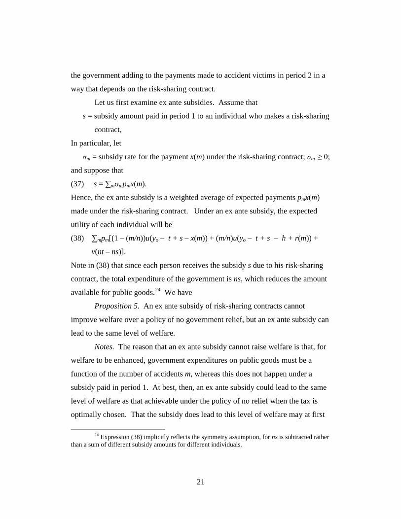
21

the government adding to the payments made to accident victims in period 2 in a

way that depends on the risk-sharing contract.

Let us first examine ex ante subsidies. Assume that

s = subsidy amount paid in period 1 to an individual who makes a risk-sharing

contract,

In particular, let

σm = subsidy rate for the payment x(m) under the risk-sharing contract; σm ≥ 0;

and suppose that

(37) s = ∑mσmpmx(m).

Hence, the ex ante subsidy is a weighted average of expected payments pmx(m)

made under the risk-sharing contract. Under an ex ante subsidy, the expected

utility of each individual will be

(38) ∑mpm[(1 – (m/n))u(yo – t + s – x(m)) + (m/n)u(yo – t + s – h + r(m)) +

v(nt – ns)].

Note in (38) that since each person receives the subsidy s due to his risk-sharing

contract, the total expenditure of the government is ns, which reduces the amount

available for public goods.24

Proposition 5. An ex ante subsidy of risk-sharing contracts cannot

improve welfare over a policy of no government relief, but an ex ante subsidy can

lead to the same level of welfare.

We have

Notes. The reason that an ex ante subsidy cannot raise welfare is that, for

welfare to be enhanced, government expenditures on public goods must be a

function of the number of accidents m, whereas this does not happen under a

subsidy paid in period 1. At best, then, an ex ante subsidy could lead to the same

level of welfare as that achievable under the policy of no relief when the tax is

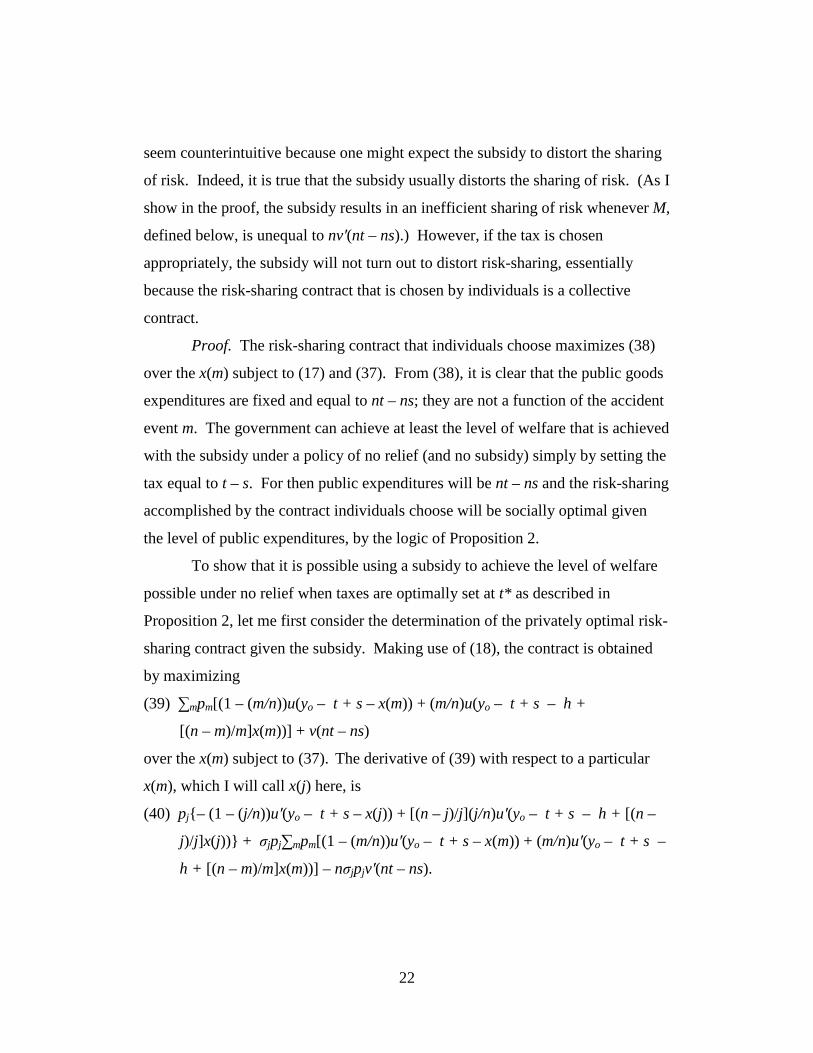
optimally chosen. That the subsidy does lead to this level of welfare may at first

24 Expression (38) implicitly reflects the symmetry assumption, for ns is subtracted rather

than a sum of different subsidy amounts for different individuals.

22

seem counterintuitive because one might expect the subsidy to distort the sharing

of risk. Indeed, it is true that the subsidy usually distorts the sharing of risk. (As I

show in the proof, the subsidy results in an inefficient sharing of risk whenever M,

defined below, is unequal to nv′(nt – ns).) However, if the tax is chosen

appropriately, the subsidy will not turn out to distort risk-sharing, essentially

because the risk-sharing contract that is chosen by individuals is a collective

contract.

Proof. The risk-sharing contract that individuals choose maximizes (38)

over the x(m) subject to (17) and (37). From (38), it is clear that the public goods

expenditures are fixed and equal to nt – ns; they are not a function of the accident

event m. The government can achieve at least the level of welfare that is achieved

with the subsidy under a policy of no relief (and no subsidy) simply by setting the

tax equal to t – s. For then public expenditures will be nt – ns and the risk-sharing

accomplished by the contract individuals choose will be socially optimal given

the level of public expenditures, by the logic of Proposition 2.

To show that it is possible using a subsidy to achieve the level of welfare

possible under no relief when taxes are optimally set at t* as described in

Proposition 2, let me first consider the determination of the privately optimal risk-

sharing contract given the subsidy. Making use of (18), the contract is obtained

by maximizing

(39) ∑mpm[(1 – (m/n))u(yo – t + s – x(m)) + (m/n)u(yo – t + s – h +

[(n – m)/m]x(m))] + v(nt – ns)

over the x(m) subject to (37). The derivative of (39) with respect to a particular

x(m), which I will call x(j) here, is

(40) pj{– (1 – (j/n))u′(yo – t + s – x(j)) + [(n – j)/j](j/n)u′(yo – t + s – h + [(n –

j)/j]x(j))} + σjpj∑mpm[(1 – (m/n))u′(yo – t + s – x(m)) + (m/n)u′(yo – t + s –

h + [(n – m)/m]x(m))] – nσjpjv′(nt – ns).

23

The first term in (40) is the direct effect of increasing x(j) on expected utility in

the accident event j; the second term is the income effect due to the increase in the

subsidy; and the third term is the reduction in public goods due to the expenditure

on the subsidy. Setting the expression in (40) equal to zero and dividing by pj

gives the first-order condition

(41) [(n – j)/j](j/n)u′(yo – t + s – h + [(n – j)/j]x(j)) + σj(M – nv′(nt – ns))

= (1 – (j/n))u′(yo – t + s – x(j)),

where M stands for ∑mpm[(1 – (m/n))u′(yo – t + s – x(m)) + (m/n)u′(yo – t + s –

h + [(n – m)/m]x(m))], the expected marginal utility of income. Condition (41)

simplifies to

(42) u′(yo – t + s – h + [(n – j)/j]x(j)) + σj[n/(n – j)](M – nv′(nt – ns)) = u′(yo – t

+ s – x(j)).

Note therefore the significance of the sign of (M – nv′(nt – ns)), the expected

marginal utility of income minus the social marginal utility from public goods. If

M > nv′(nt – ns), then u’(yo – t + s – h + [(n – j)/j]x(j)) < u’(yo – t + s – x(j)), so

that yo – t + s – h + [(n – j)/j]x(j) > yo – t + s – x(j); if M < nv′(nt – ns), then yo –

t + s – h + [(n – j)/j]x(j) < yo – t + s – x(j); and if M = nv′(nt – ns), then yo – t +

s – h + [(n – j)/j]x(j) = yo – t + s – x(j).

Now to demonstrate the claim, let

(43) s* = ∑mσmpm(m/n)h

for any subsidy scheme of the σm. This is the subsidy payment that a person would

receive if he made the optimal risk-sharing contract in the absence of relief, for

from Proposition 2 we know that x*(m) = (m/n)h. Let the tax be

(44) t** = t* + s*,

where t* is the optimal tax in Proposition 2. I assert that given t**, the same

outcome described in Proposition 2 will be implemented under the subsidy

scheme. This follows immediately from two observations: (i) If the risk-sharing

contract chosen by individuals is x*(m) = (m/n)h, then by (43) and (44), public

24

goods expenditures must be nt** – ns* = nt* and the outcome in Proposition 2

will thus be achieved. (ii) The risk-sharing contract chosen by individuals will be

x*(m), for when public goods expenditures are nt*, equation (24) must hold. In

particular, (24) states that ∑mpmu′(yo – t* – (m/n)h) = nv′(nt*). Accordingly, if

x(m) = (m/n)h, then the first-order condition (42) will be satisfied at x(m) =

(m/n)h, for then (24) means that M = nv′(nt** – ns*) = nv′(nt*). Q. E. D.

Next consider ex post subsidies of risk-sharing contracts. Under an ex

post subsidy, I assume that if m accidents occur, the government adds σm dollars

to each dollar paid under a risk-sharing contract by those who are not accident

victims. Hence, the extra amount received by each accident victim is

(45) σm(n – m)x(m)/m

and the expenditure of the government on the subsidy is

(46) σm(n – m)x(m).

Thus, an ex post subsidy resembles government relief to accident victims,

suggesting that such a subsidy can improve welfare over a policy of no relief.

The two propositions that follow validate this intuition.

Proposition 6. An ex post subsidy of risk-sharing contracts can improve

welfare over a policy of no government relief. In particular, suppose that the tax

is the optimal tax t* under the policy of no relief. Then a welfare-improving ex

post subsidy scheme exists involving a positive subsidy for accident events m

where m is sufficiently high, determined by (25), as in Proposition 3.

Notes. The logic underlying this conclusion is similar to that of

Proposition 3. Namely, when m obeys (25), the marginal utility of income

exceeds the social marginal utility of the public good, implying that a reduction in

public goods accomplished by a subsidy will be socially beneficial, other things

being equal. A complication arises, however, because subsidies tend to distort

risk-sharing. Nevertheless, as will be indicated, the first-order welfare loss due to

25

the subsidy-related distortion is zero when the subsidy begins to be applied, so

that a sufficiently small subsidy will raise welfare.

Proof. Given the definition of ex post subsidies, the expected utility of an

individual is

(47) ∑mpm[(1 – (m/n))u(yo – t – x(m)) + (m/n)u(yo – t – h + (1 + σm)[(n –

m)/m]x(m)) + v(nt – σm(n – m)x(m))],

The optimal contract maximizes (47) over the x(m). Since the choice of x(m)

affects only the mth term in (47), the problem of maximizing (47) over the x(m)

reduces to maximizing

(48) (1 – (m/n))u(yo – t – x(m)) + (m/n)u(yo – t – h + (1 + σm)[(n – m)/m]x(m)) +

v(nt – σm(n – m)x(m)).

over x(m) for each m individually. For convenience, let me write x(m) in (48) as x

and take its derivative with respect to x to obtain,

(49) –(1 – (m/n))u′(yo – t – x) + (1 + σm)[(n – m)/m](m/n)u′(yo – t – h + (1 +

σm)[(n – m)/m]x) – σm(n – m)v′(nt – σm(n – m)x).

The first-order condition determining x is thus

(50) (1 + σm)[(n – m)/m](m/n)u′(yo – t – h + (1 + σm)[(n – m)/m]x)

= (1 – (m/n))u′(yo – t – x) + σm(n – m)v′(nt – σm(n – m)x),

or, after simplification,

(51) u′(yo – t – h + (1 + σm)[(n – m)/m]x) = u′(yo – t – x)

+ σm[nv′(nt – σm(n – m)x) – u′(yo – t – h + (1 + σm)[(n – m)/m]x)].

Now suppose that t = t*, the optimal tax under the no relief policy, as

determined in Proposition 2. Choose an m sufficiently high that it is in the set G

described in Proposition 3; hence

(52) u′(yo – t* – (m/n)h) > nv′(nt*).

I claim that for this m, there exists a positive σm such that the subsidy policy with

this σm and all other σi equal to 0 results in higher welfare than the policy of no

relief. Showing this claim will obviously demonstrate that some ex post subsidy

26

policy dominates the policy of no relief. To prove the claim, it will suffice to

show that the derivative of (48) with respect to σm is positive when evaluated at σm

= 0, for all the terms in expected utility other than the mth are the same as those

under the policy of no relief since the σi are 0 for i ≠ m. Let me rewrite (48) as

follows.

(53) ω(x(σ), σ) = (1 – (m/n))u(yo – t* – x(σ)) + (m/n)u(yo – t* – h

+ (1 + σ)[(n – m)/m]x(σ)) + v(nt* – σ(n – m)x(σ)),

where ω stands for welfare when m accidents occur, σ stands for σm, and x(σ)

stands for x(m), which is a function of σm determined implicitly by (51). The

derivative of (53) with respect to σ is

(54) –x′(σ)(1 – (m/n))u′(yo – t* – x(σ))

+ (m/n)(1 + σ)[(n – m)/m]x′(σ)u′(yo – t* – h + (1 + σ)[(n – m)/m]x(σ))

+ (m/n)[(n – m)/m]x(σ)u′(yo – t* – h + (1 + σ)[(n – m)/m]x(σ))

–(n – m)x(σ)v′(nt* – σ(n – m)x(σ)) – σ(n – m)x′(σ)v′(nt* – σ(n – m)x(σ)).

Now at σ = 0, (54) is

(55) –x′(0)(1 – (m/n))u′(yo – t* – x(0))

+ (m/n)[(n – m)/m]x′(0)u′(yo – t* – h + [(n – m)/m]x(0))

+ (m/n)[(n – m)/m]x(0)u′(yo – t* – h + [(n – m)/m]x(0)) – (n – m)x(0)v′(nt*).

But at σ = 0, we know that since there is no subsidy, the risk-sharing contract is

such that x(m) = (m/n)h and the wealth of both those who suffer from accidents

and those who do not is yo – t* – (m/n)h. Hence (55) reduces to

(56) –x′(0)(1 – (m/n))u′(yo – t* – (m/n)h) + (m/n)[(n – m)/m]x′(0)u′(yo – t*

– (m/n)h) + (m/n)[(n – m)/m](m/n)hu′(yo – t* – (m/n)h) – (n – m)(m/n)hv′(nt*)

= [(n – m)/n](m/n)hu′(yo – t* – (m/n)h) – (n – m)(m/n)hv′(nt*)

= [(n - m)m/n]h[u′(yo – t* – (m/n)h)/n – v′(nt*)].

The last expression must be positive, due to (52), which completes the proof.

What was shown, that the derivative of ω(x(σ), σ) with respect to σ is positive

when evaluated at 0 may be understood as follows. The derivative equals ωx(x(σ),

27

σ)x′(σ) + ωσ(x(σ), σ). But ωx(x(σ), σ) must be zero: it is the effect on expected

utility given m of transferring wealth from nonvictims to victims starting from the

optimal contract when there is no subsidy; and under that optimal contract, wealth

for nonvictims and victims is the same, meaning that there is no first-order effect

from transferring additional wealth between them. Hence, the derivative reduces

to ωσ(x(σ), σ), the direct effect of the subsidy, which is to shift wealth from public

goods expenditures to individuals. Since m is high, in the set G guaranteeing

(52), this must be beneficial. Q. E. D.

Finally, let me show that the first-best outcome can be achieved under a

subsidy policy if the tax is raised from t*, the optimal tax under the policy of no

relief, to the level sufficiently high to allow the ideal level of public goods if there

are no accidents.

Proposition 7. Suppose that the tax is z*(0)/n. Then there exists an ex

post subsidy policy under which the first-best outcome will be achieved.

Notes. This explanation for this result is similar to that for Proposition 4.

If the tax is as stated, then tax revenues are z*(0), so the optimal level of public

goods will be supplied if there are no accidents. If there are a positive number m

of accidents, the first-best level of public goods will be achieved if the

government reduces expenditures on public goods appropriately, which will

happen if its positive subsidy rate is chosen to accomplish that objective.

However, when the subsidy rate is positive, one might expect risk-sharing to be

distorted, preventing achievement of the first-best outcome. As the proof shows,

though, risk-sharing turns out not to be distorted if the subsidy policy is chosen

optimally.

Proof. Assume that the tax t is z*(0)/n. Then when m = 0, the first-best

outcome will be achieved. Now suppose that, for any positive m, we have

(57) σm(n – m)x(m) = z*(0) – z*(m).

28

Then public goods will be first-best given m, since the left-hand side is

government expenditures on the subsidy, which will reduce government

expenditures on public goods from z*(0) to z*(m).

Suppose also that σm and x(m) are such that

(58) yo – z*(0)/n – x(m) = yo – z*(0)/n – h + [(n – m)/m](1 + σm)x(m).

This means that nonaccident victims have the same wealth as accident victims,

and thus that risk-sharing will also be first-best. Hence, if I can show that there

exist σm and x(m) satisfying (57) and (58) and that x(m) will also be chosen by

individuals—which is to say, that x(m) satisfies the first-order condition (51) —I

will have demonstrated that the first-best outcome can be achieved under an ex

post subsidy.

Note first that (57) and (58) imply that

(59) yo – z*(0)/n – x(m) = yo – z*(m)/n – (m/n)h.

This must be true, for (57) implies that the total wealth available for individuals to

consume is nyo – z*(m) – mh, which means that the per person wealth for

consumption is yo – z*(m)/n – (m/n)h, and (58) implies that each person must

consume this amount.

Now to show that (51), will be satisfied, observe that (57) and (59) imply

that (51) reduces to nv′(z*(m)) – u′(yo – z*(m)/n – (m/n)h) = 0, and this must hold

by (9).

It remains to show that there exist positive σm and x(m) obeying (57) and

(58). Solving them, we find that

(60) x(m) = (mh – (z*(0) – z*(m))/n,

(61) σm = n(z*(0) – z*(m))/[(n – m)(mh – (z*(0) – z*(m)).

These are both positive, for (15) implies that z*(0) – z*(m) < mh. Q. E. D.

2.6 Adjustment of taxes. To this point, I have discussed how government

relief for accident victims and subsidy of risk-sharing contracts can be employed

29

to raise social welfare. Another way for the government to raise social welfare is

to reduce the tax as the number of accidents increases.

Proposition 8. Suppose that the tax is imposed at time 2 and equals

z*(m)/n—or equivalently that the tax is imposed at time 1 but is adjusted at time

2, through a surtax or a credit, such that the final tax is z*(m)/n. Then the risk-

sharing contract will be x(m) = (m/n)h and r(m) = ((1 – (m/n))h, the wealth of each

individual in accident event m will be yo – z*(m)/n – (m/n)h, and the first-best

outcome will be achieved.

Notes. It is evident that there is no need for relief or subsidy of risk-

sharing if taxes depend on the number of accidents, for such adjustment of taxes

allows the level of wealth available for consumption to be a function of the

number of accidents, and privately-optimal risk sharing then results in the socially

best outcome.

Proof. The tax results in the first-best level of the public good in each

accident event m by assumption. That the risk-sharing contract is as claimed

follows essentially from the proof of Proposition 2. Hence, the first-best outcome

is achieved. Q. E. D.

3. Concluding Remarks

To recapitulate, it was shown in the world of a simple model that the

government can raise social welfare by giving aid when substantial, especially

correlated, adverse outcomes occur. The reason was that privately optimal risk-

sharing does not lead to full protection against large risks, whereas the

government can divert resources from provision of public goods to relief for

victims of adverse outcomes.

Three methods of government support were beneficial. One was direct

relief to accident victims. A second was ex post subsidy of risk-sharing

arrangements (such as federal participation in the coverage of flood insurance

30

claims25). Ex ante subsidy of risk-sharing agreements (illustrated by the

earthquake insurance program in California26), however, was not socially

advantageous because it does not lead to the shifting of government-controlled

resources to individuals as a function of the extent of accident losses. The third

type of beneficial aid was income tax adjustment in the light of accidents.27

However, these types of government aid would not be equivalent

These three forms of government help were equivalent in the sense that they

could each be employed to achieve first-best outcomes.

in the face of a number of factors that were not reflected in the model. For

example, the factor of moral hazard might be addressed better by a tailored

government-supported insurance program than by direct government relief or tax

adjustment. Conversely, problems stemming from the underestimation of risks

might be better met by direct relief or tax adjustment, as these forms of

government aid do not depend on the accuracy of individuals’ perceptions of risk.

25 The federal flood insurance program involves both ex post subsidy, in that it can resort

to borrowing from the Treasury, and ex ante subsidy of premiums. See FEMA (2002), pp. 22-28.

26 The insurance offered under the auspices of the California Earthquake Authority incorporates an implicit ex ante subsidy of premiums because the Authority does not pay taxes. However, the program of the Authority does not reflect an ex post subsidy in that it cannot draw on the state’s funds if its assets are not sufficient to pay the claims made in a large earthquake. See www.earthquakeauthority.com.

27 The income tax system in fact has a feature that gives relief from accident losses:

casualty losses may be deducted from taxable income. However, the casualty loss deduction is not conditioned on whether the losses are correlated (and thus not on the availability or price of insurance coverage).

31

References Arrow, Kenneth J., and Robert C. Lind. 1970. “Uncertainty and the Evaluation of

Public Investment Decisions.” American Economic Review, 60(3): 364-378.

Cook, Philip, and Donald Graham. 1977. “The Demand for Insurance and

Protection: The Case of Irreplaceable Commodities.” Quarterly Journal of Economics, 99(1): 143-156.

Cummins, J. David. 2006. “Should the Government Provide Insurance for

Catastrophes?” Federal Reserve Bank of St. Louis Review, 88(4): 337-379.

Dionne, Georges, Neil Doherty, and Nathalie Fombaron. 2000. “Adverse

Selection in Insurance Markets,” in Georges Dionne, ed., Handbook of Insurance. Boston: Kluwer, ch. 7.

Federal Emergency Management Agency. 2002. National Flood Insurance

Program. Program Description. http://www.fema.gov/about/programs/nfip/index.shtm.

Froot, Kenneth, ed. 1999. The Financing of Catastrophe Risk. Chicago:

University of Chicago Press. Froot, Kenneth A. 2001. “The Market for Catastrophe Risk: A Clinical

Examination.” Journal of Financial Economics, 60(2-3): 529-571. Jaffee, Dwight M., and Thomas Russell. 1997. “Catastrophe Insurance, Capital

Markets, and Uninsurable Risks.” Journal of Risk and Insurance, 64(2): 205-230.

Kaplow, Louis. 1991. “Incentives and Government Relief for Risk.” Journal of

Risk and Uncertainty, 4(2): 167-175. Kunreuther, Howard, Ginsburg, R., Miller, L., Sagi, P., Slovic, Paul, Borkin, B.,

Katz, N. 1978. Disaster Insurance Protection. New York: Wiley. Moss, David A. 1999. “Courting Disaster? The Transformation of Federal

Disaster Policy Since 1803,” in Kenneth Froot, ed., The Financing of Catastrophe Risk. Chicago: University of Chicago Press, ch. 8.

32

Priest, George L. 1996. “The Government, the Market, and the Problem of

Catastrophic Loss.” Journal of Risk and Uncertainty, 12(2-3): 219-237.