A Generalized Simulated-Annealing Optimization for Inversion of First-Arrival

Times Sathish K. Pullammanappallil and John N. Louie

Seismological Laboratory (174), Mackay School of Mines, University of Nevada, Reno

Published in Bulletin of the Seismological Society of America, Vol. 84, No. 5, pp. 1397-1409, October 1994

Abstract We employ a Monte Carlo-based optimization scheme called generalized simulated annealing to invert first-arrival times for velocities. We use "dense" common depth point (CDP) data having high multiplicity, as opposed to traditional refraction surveys with few shots. A fast finite-difference solution of the eikonal equation computes first arrival travel times through the velocity models. We test the performance of this optimization scheme on synthetic models and compare it with a linearized inversion. Our tests indicate that unlike the linear methods, the convergence of the simulated-annealing algorithm is independent of the initial model. In addition, this scheme produces a suite of "final" models having comparable least-square error. These allow us to choose a velocity model most in agreement with geological or other data. Exploiting this method's extensive sampling of the model space, we can determine the uncertainties associated with the velocities we obtain.

We use the optimization procedure on first-arrival times picked from two sets of field shot records. One is the data set from COCORP Death Valley Line 9, which traverses the central Basin and Range province in California and Nevada. The other data set is marine reflection data collected by the EDGE consortium across the Hosgri fault, offshore California. In both cases the velocities in the region undergo rapid lateral changes, and our technique images these variations with little a priori information.

Introduction We use first arrivals, including both direct and refracted phases recorded during surface seismic surveys, to obtain shallow velocity structure. By doing so, we exploit the increasing multiplicity of "refraction" surveys. Whereas early surveys were simply shot-reversed, we now have common depth point data with many shots and high multiplicity. This enables us to obtain high-resolution images of the shallow subsurface.

Determination of near-surface velocities is important for geological, geophysical, and engineering studies. The effect of the low-velocity weathering layer has to be accounted for in engineering site investigations (eg.: Hatherly and Neville, 1986). Lateral velocity variations in this layer contaminate stacked seismic sections and introduce apparent structure on deeper reflection events. These are removedby "statics'' corrections, which need accurate velocity

estimates (Farrell and Euwema, 1984; Russell, 1989). Shallow velocity structure determined from refraction times have been used for groundwater studies (eg.: Haeni, 1986). In addition, imaging near-surface crustal structure is important in neotectonic studies of a region (eg.: Geist and Brocher, 1987).

Various schemes are employed to determine refraction velocities. Layered velocity models can be obtained using, for example, the Herglotz-Wiechert formula (Gerver and Markushevitch, 1966), wavefront methods (Thornburgh, 1930; Rockwell, 1967), or the plus-minus method (Hagedoorn, 1959). Palmer (1981) and Jones and Jovanovich (1985) describe methods to derive the depth to an irregular refractor as well as lateral velocity changes along the refractor. Clayton and McMechan (1981) and McMechan et. al. (1982) use a wave field transformation approach, that avoids preprocessing of the data, to invert refraction data for a velocity profile. Several workers, for example, Hampson and Russell (1984), de Amorim et al. (1987), Olsen (1989), Docherty (1992), and Simmons and Backus (1992) employ linearized inversion schemes to invert first-arrival times for near-surface velocities. Travel time inversion is a nonlinear process because a perturbation in the velocity field results in changes in the ray paths through it. Linearized inversions involve local linearization of this nonlinear problem. This makes them initial-model dependent, and a poor choice of the starting model could cause the inversion to converge to an incorrect solution at a local minimum.

To circumvent this problem, we demonstrate the use of a nonlinear optimization technique, namely a generalized simulated annealing, to invert first-arrival times for shallow velocities. We rapidly compute travel times through models by a method avoiding ray tracing. It employs a fast finite-difference scheme based on a solution to the eikonal equation (Vidale, 1988). This accounts for curved rays and all types of primary arrivals, be they direct arrivals, refractions, or diffractions. We test the optimization process on synthetic models that mimic typical geological cross-sections encountered in the field. We compare its performance with a linearized inversion and demonstrate the initial-model dependence of the latter.

Velocities obtained from refraction studies find wide use in statics corrections (i.e., to remove near-surface effects interfering with deeper reflections). To test the utility of our method for statics correction we compute vertical travel times through the models obtained. This also serves to compare the robustness of the inversion results using the different methods. Another advantage of the simulated-annealing algorithm is that it produces a suite of final models having comparable least-square error. This enables us to choose models most likely to represent the geology of a region. We also use this property to determine the uncertainties associated with the model velocities obtained.

We use this technique on two different data sets to obtain velocity information of the crust at relatively shallow horizons. The first data set is COCORP Death Valley line 9, which traverses the central Basin and Range province. Accurate velocity models in this region are necessary to test models that can explain the observed extreme crustal extension. The second data set is shot gathers recorded by the EDGE consortium across the Hosgri fault (RU-3 line), offshore California. We use the nonlinear optimization technique to obtain a high-resolution velocity structure in this region, with minimum a priori constraints. The only constraints that go into our method are the size of the model and the minimum and maximum crustal velocities one is likely to encounter in the region. We then use it in a pre-stack Kirchhoff-sum migration that accounts for curved rays, to accurately image the Hosgri fault.

Simulated-Annealing Optimization The simulated annealing method of optimization has been used widely to tackle geophysical problems. It has been used in estimating residual statics corrections for seismic reflection surveys (Rothman, 1985; Vasudevan et al., 1991), coherency optimization for reflection problems (Landa et al., 1989), transmission tomography (Ammon and Vidale, 1993), and one-dimensional seismic waveform inversion (Sen and Stoffa, 1991), to name a few. Having data that leaves many parameters poorly determined in the models we construct motivates us to use an optimization by forward modeling. We will demonstrate that a modeling approach is much more robust than inversions.

Our implementation follows the method described by Bohachevsky et al. (1986), called generalized simulated annealing. Its basis is a Monte Carlo technique due to Metropolis et al. (1953). We detail our implementation below:

1. Compute travel times through an initial model. Determine the least-square error, E0. For any iteration i, we can define the least-square error, which is the objective function, as:

Ei = (1/n)(Σ(tjobs - tj cal)2), (1)

where n is the number of observations, j denotes each observation and tobs and tcal are the observed (data) and calculated traveltimes respectively. The summation goes from j=1 to j=n.

2. We perturb the velocity model by adding random constant-velocity boxes, followed by smoothing by averaging over each four adjacent cells, to avoid imposing any unjustified precision on our models. During the optimization, the added boxes can assume any velocity between two fixed values chosen by the user. The boxes can have any aspect ratio and vary between one cell size and the entire model size. Thus, we can easily adapt the process of guessing new models to fit any constraints or a priori information. The bounds we use in perturbing velocities constitute such a priori information that makes this optimization more stable and robust than many inversions. We demonstrate this later in our comparisons with an inversion scheme that uses smoothing as a damping factor.

We next compute the new least-square error E1.

3. The new model is unconditionally accepted if its error is smaller (E1 <= E0 ), and conditionally accepted with a probability:

Pc = exp{( Emin - E1 ) q ΔE / T} (2)

when E1 > E0 . In the above equation, ΔE = E0 - E1, T is called the temperature, q is an empirical parameter, and Emin is the value of the objective function at the global minimum (ideally, equal to zero). Conditional acceptance of models with larger least square error enables the algorithm to escape out of local minima in its search for the global minimum. The

factor ( Emin - E1 ) q makes the probability of accepting a detrimental step towards local minima tend to zero as the inversion approaches the global minimum.

4. We repeat steps 2 through 4 until the optimization converges. Our criterion for convergence requires the difference in least-square error between successive models and the probability of accepting new models having greater error to become very small. We discern the latter condition when there are a large number of iterations (50,000 or more, or an order of magnitude larger than the number of model parameters) over which no model is accepted.

From equation (2), we see that the convergence of the optimization scheme depends on two empirical parameters, namely q and T. Rothman (1986) and other workers have shown that the convergence of simulated annealing is sensitive to the rate of cooling, or in other words, the variation of T with iteration. The higher the temperature T, the greater the probability of accepting models with a positive ΔE , and vice-versa. So one has to design a cooling schedule to allow the algorithm to jump out of local minima during the initial stages of the optimization, yet let it converge to the global minimum during the final stages. Rapid cooling would trap the optimization in a local minimum (seen by setting T = 0 in equation (2)). Letting the temperature remain high for a large number of iterations slows the speed of convergence. To choose an optimal cooling schedule we use a procedure based on the one developed by Basu and Frazer (1990). This is described in detail in Pullammanappallil and Louie (1993). It essentially comprises numerous short runs of the algorithm for various fixed temperature values and computing the average least-square error for each run. This is then used to determine a critical temperature, Tc (Figure 1a). During the actual optimization we start at a high temperature, T, so that any bias in the initial model will be destroyed. The value of T is kept fixed for the next 1000 iterations, after which it is changed to T/10, i.e., Tnext = Tprevious/10 (Figure 1b). Keeping the temperature fixed for several iterations allows the system to reach a simulated thermal equilibrium. This facilitates better convergence. This procedure is followed until we reach the critical temperature, Tc. Then the rate at which the value of T is reduced is decreased, allowing the optimization to settle into a global minimum. Now, T is reduced only by a factor of 2 after every 10,000 iterations, i.e., Tnext = Tprevious/2 (Figure 1b).

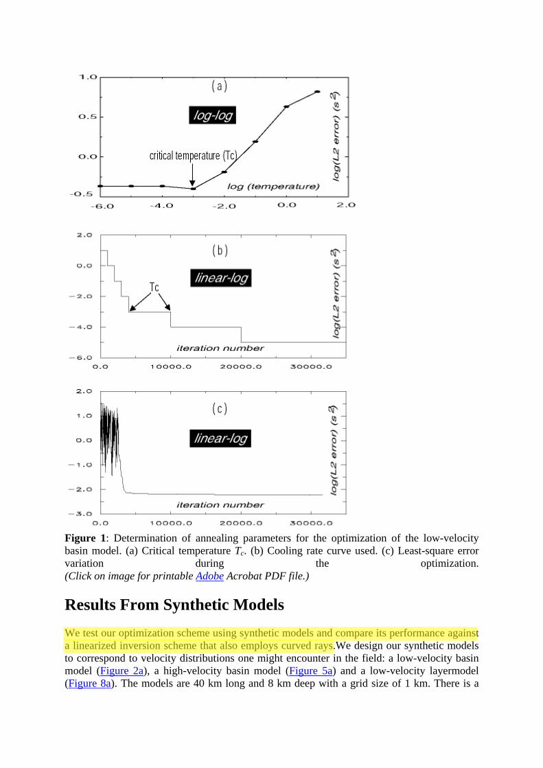
Figure 1: Determination of annealing parameters for the optimization of the low-velocity basin model. (a) Critical temperature Tc. (b) Cooling rate curve used. (c) Least-square error variation during the optimization. (Click on image for printable Adobe Acrobat PDF file.)

Results From Synthetic Models We test our optimization scheme using synthetic models and compare its performance against a linearized inversion scheme that also employs curved rays.We design our synthetic models to correspond to velocity distributions one might encounter in the field: a low-velocity basin model (Figure 2a), a high-velocity basin model (Figure 5a) and a low-velocity layermodel (Figure 8a). The models are 40 km long and 8 km deep with a grid size of 1 km. There is a

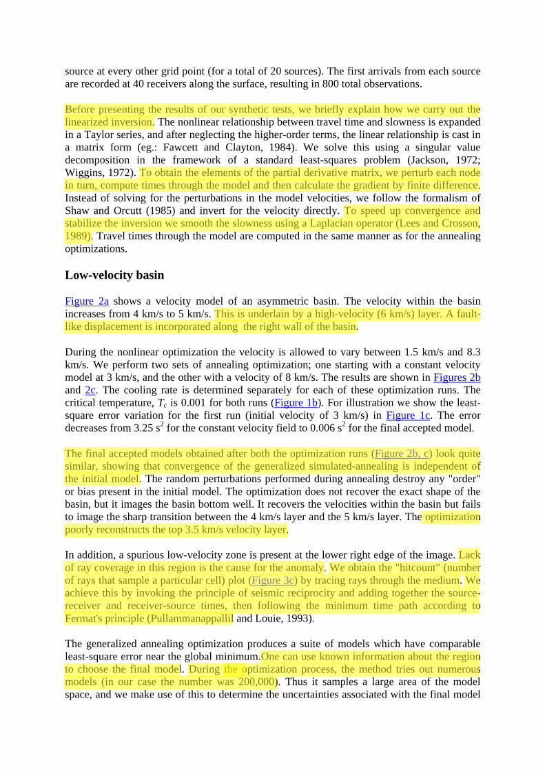
source at every other grid point (for a total of 20 sources). The first arrivals from each source are recorded at 40 receivers along the surface, resulting in 800 total observations.

Before presenting the results of our synthetic tests, we briefly explain how we carry out the linearized inversion. The nonlinear relationship between travel time and slowness is expanded in a Taylor series, and after neglecting the higher-order terms, the linear relationship is cast in a matrix form (eg.: Fawcett and Clayton, 1984). We solve this using a singular value decomposition in the framework of a standard least-squares problem (Jackson, 1972; Wiggins, 1972). To obtain the elements of the partial derivative matrix, we perturb each node in turn, compute times through the model and then calculate the gradient by finite difference. Instead of solving for the perturbations in the model velocities, we follow the formalism of Shaw and Orcutt (1985) and invert for the velocity directly. To speed up convergence and stabilize the inversion we smooth the slowness using a Laplacian operator (Lees and Crosson, 1989). Travel times through the model are computed in the same manner as for the annealing optimizations.

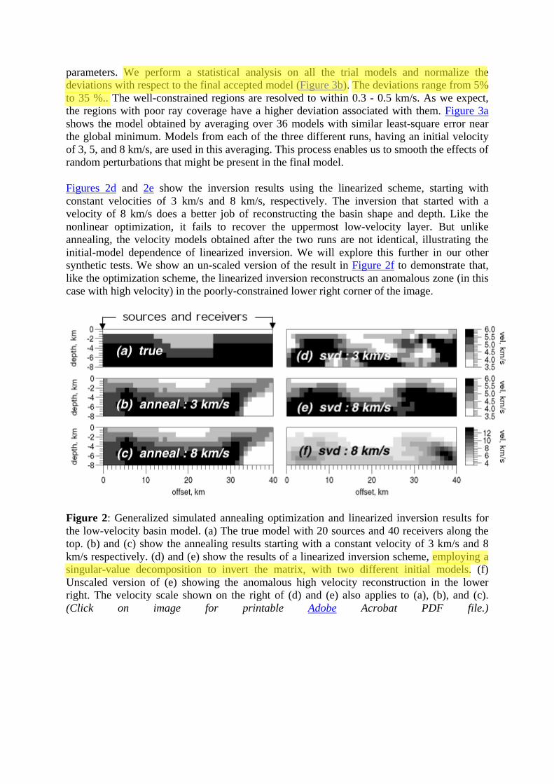
Low-velocity basin Figure 2a shows a velocity model of an asymmetric basin. The velocity within the basin increases from 4 km/s to 5 km/s. This is underlain by a high-velocity (6 km/s) layer. A fault-like displacement is incorporated along the right wall of the basin.

During the nonlinear optimization the velocity is allowed to vary between 1.5 km/s and 8.3 km/s. We perform two sets of annealing optimization; one starting with a constant velocity model at 3 km/s, and the other with a velocity of 8 km/s. The results are shown in Figures 2b and 2c. The cooling rate is determined separately for each of these optimization runs. The critical temperature, Tc is 0.001 for both runs (Figure 1b). For illustration we show the least-square error variation for the first run (initial velocity of 3 km/s) in Figure 1c. The error decreases from 3.25 s2 for the constant velocity field to 0.006 s2 for the final accepted model.

The final accepted models obtained after both the optimization runs (Figure 2b, c) look quite similar, showing that convergence of the generalized simulated-annealing is independent of the initial model. The random perturbations performed during annealing destroy any "order" or bias present in the initial model. The optimization does not recover the exact shape of the basin, but it images the basin bottom well. It recovers the velocities within the basin but fails to image the sharp transition between the 4 km/s layer and the 5 km/s layer. The optimization poorly reconstructs the top 3.5 km/s velocity layer.

In addition, a spurious low-velocity zone is present at the lower right edge of the image. Lack of ray coverage in this region is the cause for the anomaly. We obtain the "hitcount" (number of rays that sample a particular cell) plot (Figure 3c) by tracing rays through the medium. We achieve this by invoking the principle of seismic reciprocity and adding together the source-receiver and receiver-source times, then following the minimum time path according to Fermat's principle (Pullammanappallil and Louie, 1993).

The generalized annealing optimization produces a suite of models which have comparable least-square error near the global minimum.One can use known information about the region to choose the final model. During the optimization process, the method tries out numerous models (in our case the number was 200,000). Thus it samples a large area of the model space, and we make use of this to determine the uncertainties associated with the final model

parameters. We perform a statistical analysis on all the trial models and normalize the deviations with respect to the final accepted model (Figure 3b). The deviations range from 5% to 35 %.. The well-constrained regions are resolved to within 0.3 - 0.5 km/s. As we expect, the regions with poor ray coverage have a higher deviation associated with them. Figure 3a shows the model obtained by averaging over 36 models with similar least-square error near the global minimum. Models from each of the three different runs, having an initial velocity of 3, 5, and 8 km/s, are used in this averaging. This process enables us to smooth the effects of random perturbations that might be present in the final model.

Figures 2d and 2e show the inversion results using the linearized scheme, starting with constant velocities of 3 km/s and 8 km/s, respectively. The inversion that started with a velocity of 8 km/s does a better job of reconstructing the basin shape and depth. Like the nonlinear optimization, it fails to recover the uppermost low-velocity layer. But unlike annealing, the velocity models obtained after the two runs are not identical, illustrating the initial-model dependence of linearized inversion. We will explore this further in our other synthetic tests. We show an un-scaled version of the result in Figure 2f to demonstrate that, like the optimization scheme, the linearized inversion reconstructs an anomalous zone (in this case with high velocity) in the poorly-constrained lower right corner of the image.

Figure 2: Generalized simulated annealing optimization and linearized inversion results for the low-velocity basin model. (a) The true model with 20 sources and 40 receivers along the top. (b) and (c) show the annealing results starting with a constant velocity of 3 km/s and 8 km/s respectively. (d) and (e) show the results of a linearized inversion scheme, employing a singular-value decomposition to invert the matrix, with two different initial models. (f) Unscaled version of (e) showing the anomalous high velocity reconstruction in the lower right. The velocity scale shown on the right of (d) and (e) also applies to (a), (b), and (c). (Click on image for printable Adobe Acrobat PDF file.)

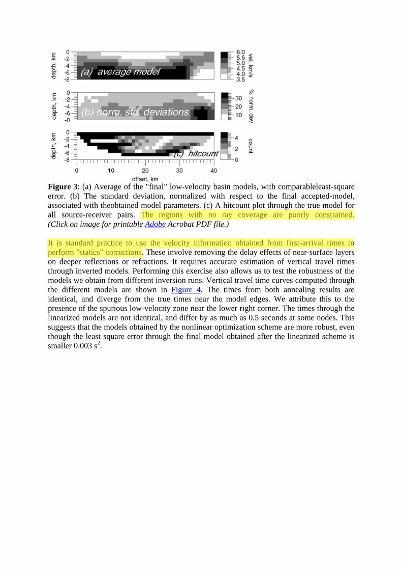
Figure 3: (a) Average of the "final" low-velocity basin models, with comparableleast-square error. (b) The standard deviation, normalized with respect to the final accepted-model, associated with theobtained model parameters. (c) A hitcount plot through the true model for all source-receiver pairs. The regions with no ray coverage are poorly constrained. (Click on image for printable Adobe Acrobat PDF file.)

It is standard practice to use the velocity information obtained from first-arrival times to perform "statics" corrections. These involve removing the delay effects of near-surface layers on deeper reflections or refractions. It requires accurate estimation of vertical travel times through inverted models. Performing this exercise also allows us to test the robustness of the models we obtain from different inversion runs. Vertical travel time curves computed through the different models are shown in Figure 4. The times from both annealing results are identical, and diverge from the true times near the model edges. We attribute this to the presence of the spurious low-velocity zone near the lower right corner. The times through the linearized models are not identical, and differ by as much as 0.5 seconds at some nodes. This suggests that the models obtained by the nonlinear optimization scheme are more robust, even though the least-square error through the final model obtained after the linearized scheme is smaller 0.003 s2.

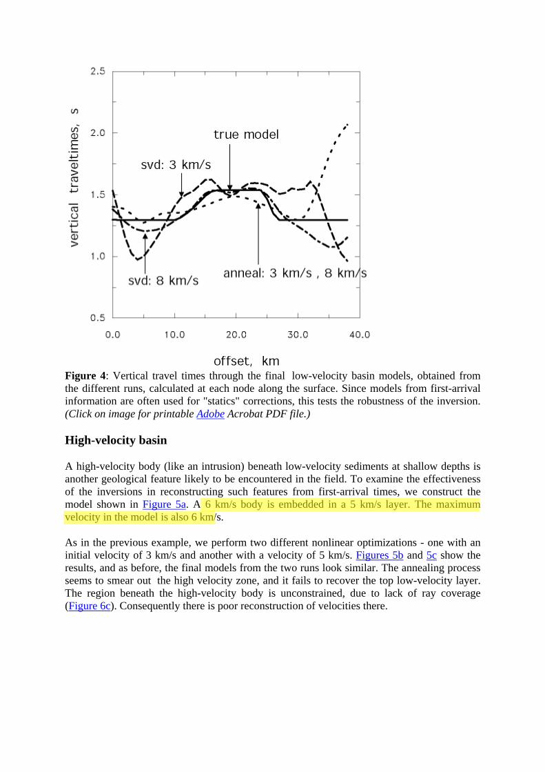
Figure 4: Vertical travel times through the final low-velocity basin models, obtained from the different runs, calculated at each node along the surface. Since models from first-arrival information are often used for "statics" corrections, this tests the robustness of the inversion. (Click on image for printable Adobe Acrobat PDF file.)

High-velocity basin

A high-velocity body (like an intrusion) beneath low-velocity sediments at shallow depths is another geological feature likely to be encountered in the field. To examine the effectiveness of the inversions in reconstructing such features from first-arrival times, we construct the model shown in Figure 5a. A 6 km/s body is embedded in a 5 km/s layer. The maximum velocity in the model is also 6 km/s.

As in the previous example, we perform two different nonlinear optimizations - one with an initial velocity of 3 km/s and another with a velocity of 5 km/s. Figures 5b and 5c show the results, and as before, the final models from the two runs look similar. The annealing process seems to smear out the high velocity zone, and it fails to recover the top low-velocity layer. The region beneath the high-velocity body is unconstrained, due to lack of ray coverage (Figure 6c). Consequently there is poor reconstruction of velocities there.

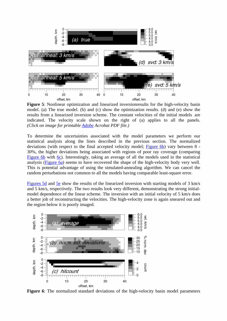
Figure 5: Nonlinear optimization and linearized inversionresults for the high-velocity basin model. (a) The true model. (b) and (c) show the optimization results. (d) and (e) show the results from a linearized inversion scheme. The constant velocities of the initial models are indicated. The velocity scale shown on the right of (a) applies to all the panels. (Click on image for printable Adobe Acrobat PDF file.)

To determine the uncertainties associated with the model parameters we perform our statistical analysis along the lines described in the previous section. The normalized deviations (with respect to the final accepted velocity model; Figure 6b) vary between 8 - 30%, the higher deviations being associated with regions of poor ray coverage (comparing Figure 6b with 6c). Interestingly, taking an average of all the models used in the statistical analysis (Figure 6a) seems to have recovered the shape of the high-velocity body very well. This is potential advantage of using the simulated-annealing algorithm. We can cancel the random perturbations not common to all the models having comparable least-square error.

Figures 5d and 5e show the results of the linearized inversion with starting models of 3 km/s and 5 km/s, respectively. The two results look very different, demonstrating the strong initial-model dependence of the linear scheme. The inversion with an initial velocity of 5 km/s does a better job of reconstructing the velocities. The high-velocity zone is again smeared out and the region below it is poorly imaged.

Figure 6: The normalized standard deviations of the high-velocity basin model parameters

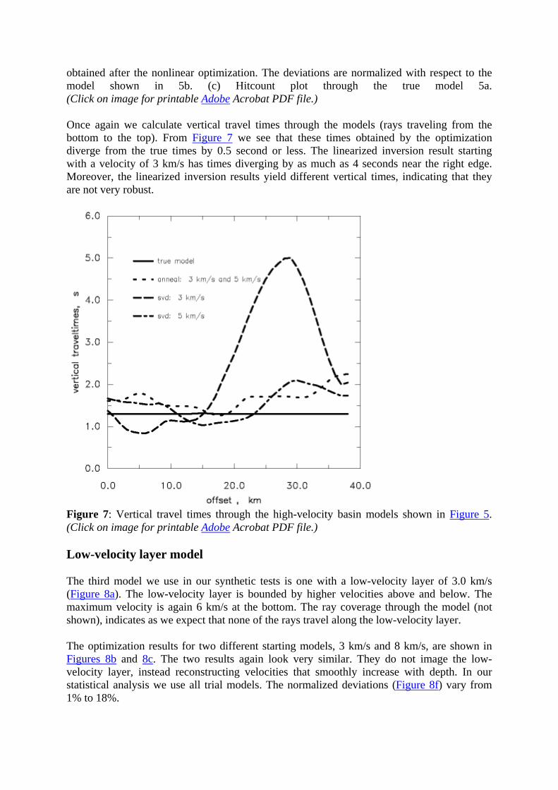
obtained after the nonlinear optimization. The deviations are normalized with respect to the model shown in 5b. (c) Hitcount plot through the true model 5a. (Click on image for printable Adobe Acrobat PDF file.)

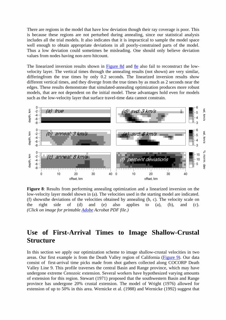
Once again we calculate vertical travel times through the models (rays traveling from the bottom to the top). From Figure 7 we see that these times obtained by the optimization diverge from the true times by 0.5 second or less. The linearized inversion result starting with a velocity of 3 km/s has times diverging by as much as 4 seconds near the right edge. Moreover, the linearized inversion results yield different vertical times, indicating that they are not very robust.

Figure 7: Vertical travel times through the high-velocity basin models shown in Figure 5. (Click on image for printable Adobe Acrobat PDF file.)

Low-velocity layer model

The third model we use in our synthetic tests is one with a low-velocity layer of 3.0 km/s (Figure 8a). The low-velocity layer is bounded by higher velocities above and below. The maximum velocity is again 6 km/s at the bottom. The ray coverage through the model (not shown), indicates as we expect that none of the rays travel along the low-velocity layer.

The optimization results for two different starting models, 3 km/s and 8 km/s, are shown in Figures 8b and 8c. The two results again look very similar. They do not image the low-velocity layer, instead reconstructing velocities that smoothly increase with depth. In our statistical analysis we use all trial models. The normalized deviations (Figure 8f) vary from 1% to 18%.

There are regions in the model that have low deviation though their ray coverage is poor. This is because these regions are not perturbed during annealing, since our statistical analysis includes all the trial models. It also indicates that it is impractical to sample the model space well enough to obtain appropriate deviations in all poorly-constrained parts of the model. Thus a low deviation could sometimes be misleading. One should only believe deviation values from nodes having non-zero hitcount.

The linearized inversion results shown in Figure 8d and 8e also fail to reconstruct the low-velocity layer. The vertical times through the annealing results (not shown) are very similar, differingfrom the true times by only 0.2 seconds. The linearized inversion results show different vertical times, and they diverge from the true times by as much as 2 seconds near the edges. These results demonstrate that simulated-annealing optimization produces more robust models, that are not dependent on the initial model. These advantages hold even for models such as the low-velocity layer that surface travel-time data cannot constrain.

Figure 8: Results from performing annealing optimization and a linearized inversion on the low-velocity layer model shown in (a). The velocities used in the starting model are indicated. (f) showsthe deviations of the velocities obtained by annealing (b, c). The velocity scale on the right side of (d) and (e) also applies to (a), (b), and (c). (Click on image for printable Adobe Acrobat PDF file.)

Use of First-Arrival Times to Image Shallow-Crustal Structure

In this section we apply our optimization scheme to image shallow-crustal velocities in two areas. Our first example is from the Death Valley region of California (Figure 9). Our data consist of first-arrival time picks made from shot gathers collected along COCORP Death Valley Line 9. This profile traverses the central Basin and Range province, which may have undergone extreme Cenozoic extension. Several workers have hypothesized varying amounts of extension for this region. Stewart (1971) proposed that the southwestern Basin and Range province has undergone 20% crustal extension. The model of Wright (1976) allowed for extension of up to 50% in this area. Wernicke et al. (1988) and Wernicke (1992) suggest that

the region must have undergone more than 100% east-west extension. Hence, imaging velocities and the shape of basins in the shallow crust is important to testing these extensional models. The velocity distribution could also offer clues on extensional mechanisms. In this paper we present only the velocity models obtained by our optimization scheme for Line 9, crossing central Death Valley. The geologic interpretation of the results and analysis of other COCORP Lines (10 and 11) in this region are the subjects of another manuscript (Pullammanappallil et al., 1993).

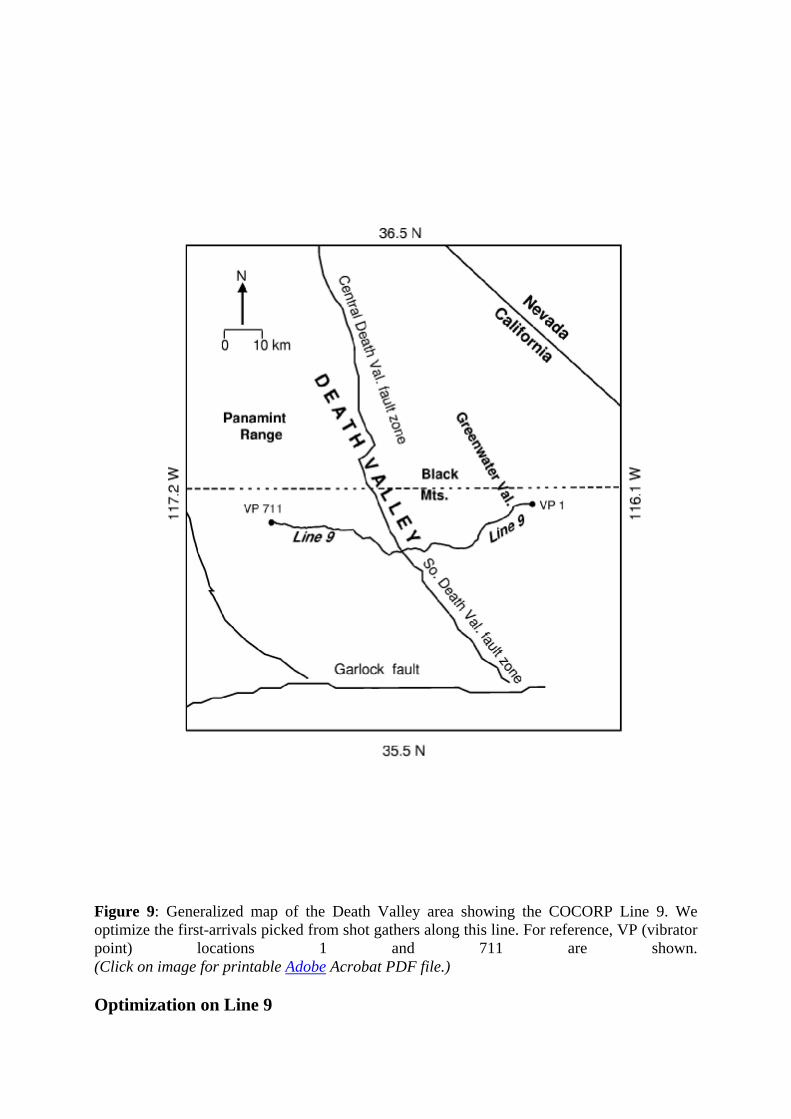
Figure 9: Generalized map of the Death Valley area showing the COCORP Line 9. We optimize the first-arrivals picked from shot gathers along this line. For reference, VP (vibrator point) locations 1 and 711 are shown. (Click on image for printable Adobe Acrobat PDF file.)

Optimization on Line 9

Line 9 traverses from the Dublin Hills in the east to the Panamint Mountains in the west (Figure 9) and cuts across several alluvial valleys. We use a total of 6213 first-arrival times picked from 281 shot gathers. To overcome the effect of bends in the profile, we project the source locations to a line while maintaining the true offsets of the source-receiver pairs. Thus the velocities we obtain from the optimization will show some lateral smearing. The maximum source-receiver offset of the survey is 10 km.

For our optimizations we use a model that is 62 km long and 5 km deep, with a grid spacing of 500 m. There is significant topography along the profile. We include elevation information by extrapolating the times to sources and receivers not on grid points. For this we assume plane-wave incidence at the receivers (pers. comm. with C. Ammon, 1991). The initial model has a constant velocity of 2 km/s. Velocity is allowed to vary between 1.5 and 8 km/s during the annealing procedure. We fix the empirical annealing constants by performing a series of short runs as described in the methods section. In this case we found the critical temperature to be 0.01.

Figure 10a shows the result of the optimization. The least-square error went from 1.51s2 for the constant velocity model to 0.007s2 for the final model. The low-velocity regions in the final model are associated with alluvial basins while the shallow high velocities show the basement rocks below mountain ranges. The prominent basin around VP 450 - 525 corresponds to central Death Valley. The Black Mountains and the Panamint Range have relatively higher velocities (4.5 - 5 km/s) beneath them.

These velocities compare very well with the forward modeling results of Geist and Brocher (1987, their Figure 4). As in the case of the synthetic examples, we obtain the model velocity uncertainties. The deviations range from 0 to 45% of the average model (Figure 10c). Figure 10b shows the average model. We plot the hitcount of the rays through the final model in Figure 10d to allow us to see that the regions with higher deviation also have poor ray coverage.

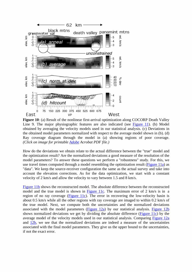
Figure 10: (a) Result of the nonlinear first-arrival optimization along COCORP Death Valley Line 9. The major physiographic features are also indicated (see Figure 11). (b) Model obtained by averaging the velocity models used in our statistical analysis. (c) Deviations in the obtained model parameters normalized with respect to the average model shown in (b). (d) Ray coverage diagram through the model in (a) showing regions of poor coverage. (Click on image for printable Adobe Acrobat PDF file.)

How do the deviations we obtain relate to the actual difference between the "true" model and the optimization result? Are the normalized deviations a good measure of the resolution of the model parameters? To answer these questions we perform a "robustness" study. For this, we use travel times computed through a model resembling the optimization result (Figure 11a) as "data". We keep the source-receiver configuration the same as the actual survey and take into account the elevation corrections. As for the data optimization, we start with a constant velocity of 2 km/s and allow the velocity to vary between 1.5 and 8 km/s.

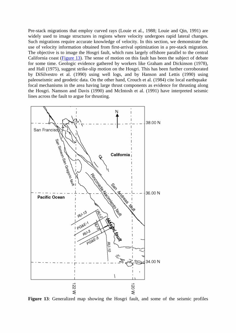
Figure 11b shows the reconstructed model. The absolute difference between the reconstructed model and the true model is shown in Figure 11c. The maximum error of 2 km/s is in a region of no ray coverage (Figure 11c). The error in recovering the low-velocity basin is about 0.5 km/s while all the other regions with ray coverage are imaged to within 0.2 km/s of the true model. Next, we compute both the uncertainties and the normalized deviations associated with the model parameters (Figure 12a) by our statistical analysis. Figure 12b shows normalized deviations we get by dividing the absolute difference (Figure 11c) by the average model of the velocity models used in our statistical analysis. Comparing Figure 12a and 12b, we see that the normalized deviations are indeed a measure of the uncertainties associated with the final model parameters. They give us the upper bound to the uncertainties, if not the exact error.

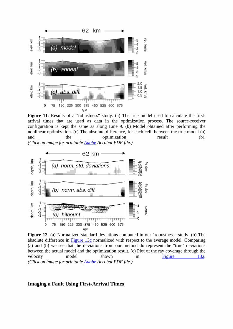
Figure 11: Results of a "robustness" study. (a) The true model used to calculate the first-arrival times that are used as data in the optimization process. The source-receiver configuration is kept the same as along Line 9. (b) Model obtained after performing the nonlinear optimization. (c) The absolute difference, for each cell, between the true model (a) and the optimization result (b). (Click on image for printable Adobe Acrobat PDF file.)

Figure 12: (a) Normalized standard deviations computed in our "robustness" study. (b) The absolute difference in Figure 13c normalized with respect to the average model. Comparing (a) and (b) we see that the deviations from our method do represent the "true" deviations between the actual model and the optimization result. (c) Plot of the ray coverage through the velocity model shown in Figure 13a. (Click on image for printable Adobe Acrobat PDF file.)

Imaging a Fault Using First-Arrival Times

Pre-stack migrations that employ curved rays (Louie et al., 1988; Louie and Qin, 1991) are widely used to image structures in regions where velocity undergoes rapid lateral changes. Such migrations require accurate knowledge of velocity. In this section, we demonstrate the use of velocity information obtained from first-arrival optimization in a pre-stack migration. The objective is to image the Hosgri fault, which runs largely offshore parallel to the central California coast (Figure 13). The sense of motion on this fault has been the subject of debate for some time. Geologic evidence gathered by workers like Graham and Dickinson (1978), and Hall (1975), suggest strike-slip motion on the Hosgri. This has been further corroborated by DiSilvestro et al. (1990) using well logs, and by Hanson and Lettis (1990) using paleoseismic and geodetic data. On the other hand, Crouch et al. (1984) cite local earthquake focal mechanisms in the area having large thrust components as evidence for thrusting along the Hosgri. Namson and Davis (1990) and McIntosh et al. (1991) have interpreted seismic lines across the fault to argue for thrusting.

Figure 13: Generalized map showing the Hosgri fault, and some of the seismic profiles

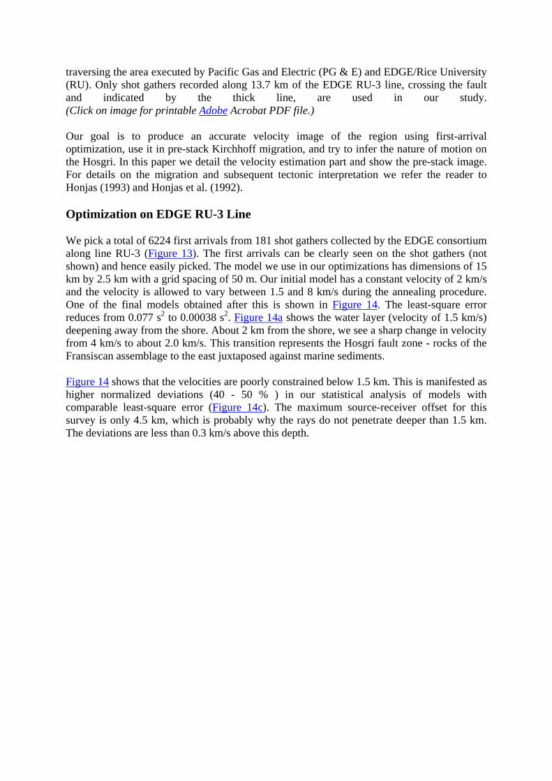
traversing the area executed by Pacific Gas and Electric (PG & E) and EDGE/Rice University (RU). Only shot gathers recorded along 13.7 km of the EDGE RU-3 line, crossing the fault and indicated by the thick line, are used in our study. (Click on image for printable Adobe Acrobat PDF file.)

Our goal is to produce an accurate velocity image of the region using first-arrival optimization, use it in pre-stack Kirchhoff migration, and try to infer the nature of motion on the Hosgri. In this paper we detail the velocity estimation part and show the pre-stack image. For details on the migration and subsequent tectonic interpretation we refer the reader to Honjas (1993) and Honjas et al. (1992).

Optimization on EDGE RU-3 Line

We pick a total of 6224 first arrivals from 181 shot gathers collected by the EDGE consortium along line RU-3 (Figure 13). The first arrivals can be clearly seen on the shot gathers (not shown) and hence easily picked. The model we use in our optimizations has dimensions of 15 km by 2.5 km with a grid spacing of 50 m. Our initial model has a constant velocity of 2 km/s and the velocity is allowed to vary between 1.5 and 8 km/s during the annealing procedure. One of the final models obtained after this is shown in Figure 14. The least-square error reduces from 0.077 s2 to 0.00038 s2. Figure 14a shows the water layer (velocity of 1.5 km/s) deepening away from the shore. About 2 km from the shore, we see a sharp change in velocity from 4 km/s to about 2.0 km/s. This transition represents the Hosgri fault zone - rocks of the Fransiscan assemblage to the east juxtaposed against marine sediments.

Figure 14 shows that the velocities are poorly constrained below 1.5 km. This is manifested as higher normalized deviations (40 - 50 % ) in our statistical analysis of models with comparable least-square error (Figure 14c). The maximum source-receiver offset for this survey is only 4.5 km, which is probably why the rays do not penetrate deeper than 1.5 km. The deviations are less than 0.3 km/s above this depth.

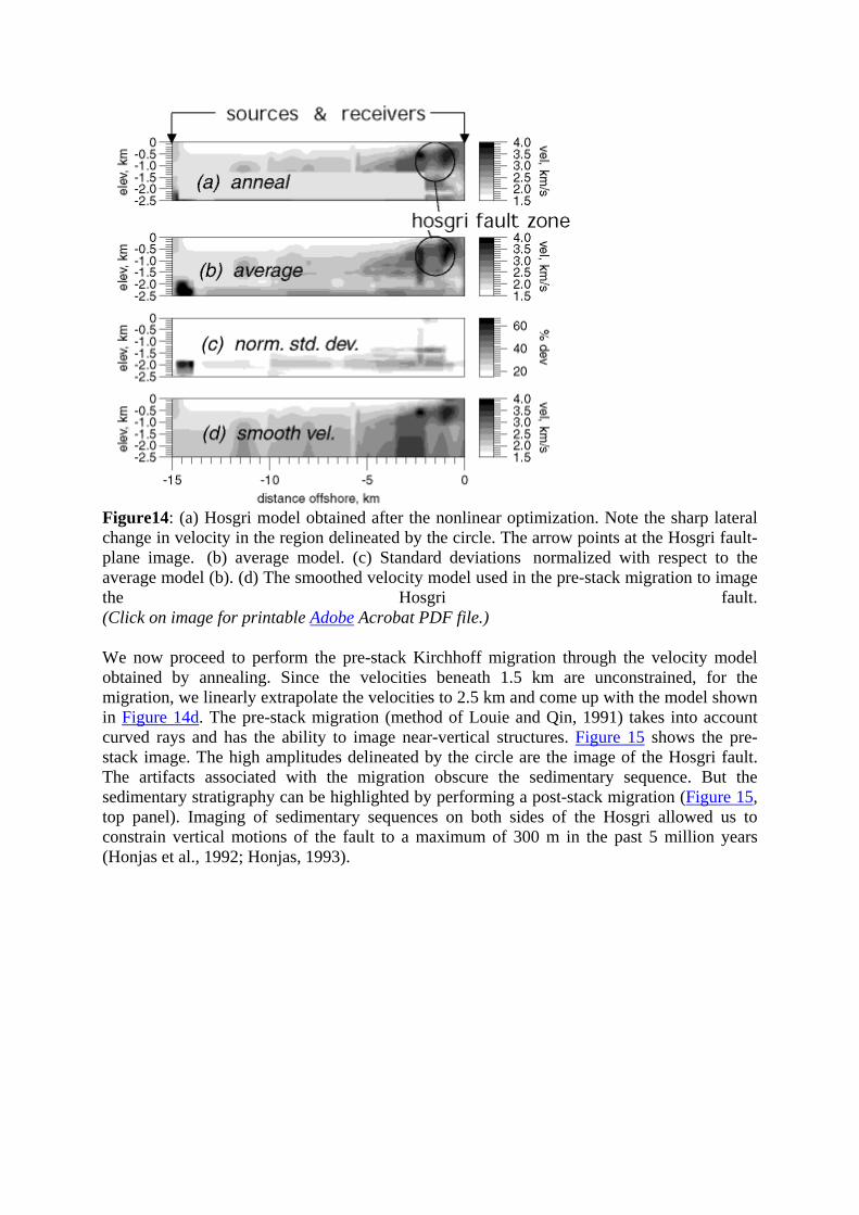
Figure14: (a) Hosgri model obtained after the nonlinear optimization. Note the sharp lateral change in velocity in the region delineated by the circle. The arrow points at the Hosgri fault-plane image. (b) average model. (c) Standard deviations normalized with respect to the average model (b). (d) The smoothed velocity model used in the pre-stack migration to image the Hosgri fault. (Click on image for printable Adobe Acrobat PDF file.)

We now proceed to perform the pre-stack Kirchhoff migration through the velocity model obtained by annealing. Since the velocities beneath 1.5 km are unconstrained, for the migration, we linearly extrapolate the velocities to 2.5 km and come up with the model shown in Figure 14d. The pre-stack migration (method of Louie and Qin, 1991) takes into account curved rays and has the ability to image near-vertical structures. Figure 15 shows the pre-stack image. The high amplitudes delineated by the circle are the image of the Hosgri fault. The artifacts associated with the migration obscure the sedimentary sequence. But the sedimentary stratigraphy can be highlighted by performing a post-stack migration (Figure 15, top panel). Imaging of sedimentary sequences on both sides of the Hosgri allowed us to constrain vertical motions of the fault to a maximum of 300 m in the past 5 million years (Honjas et al., 1992; Honjas, 1993).

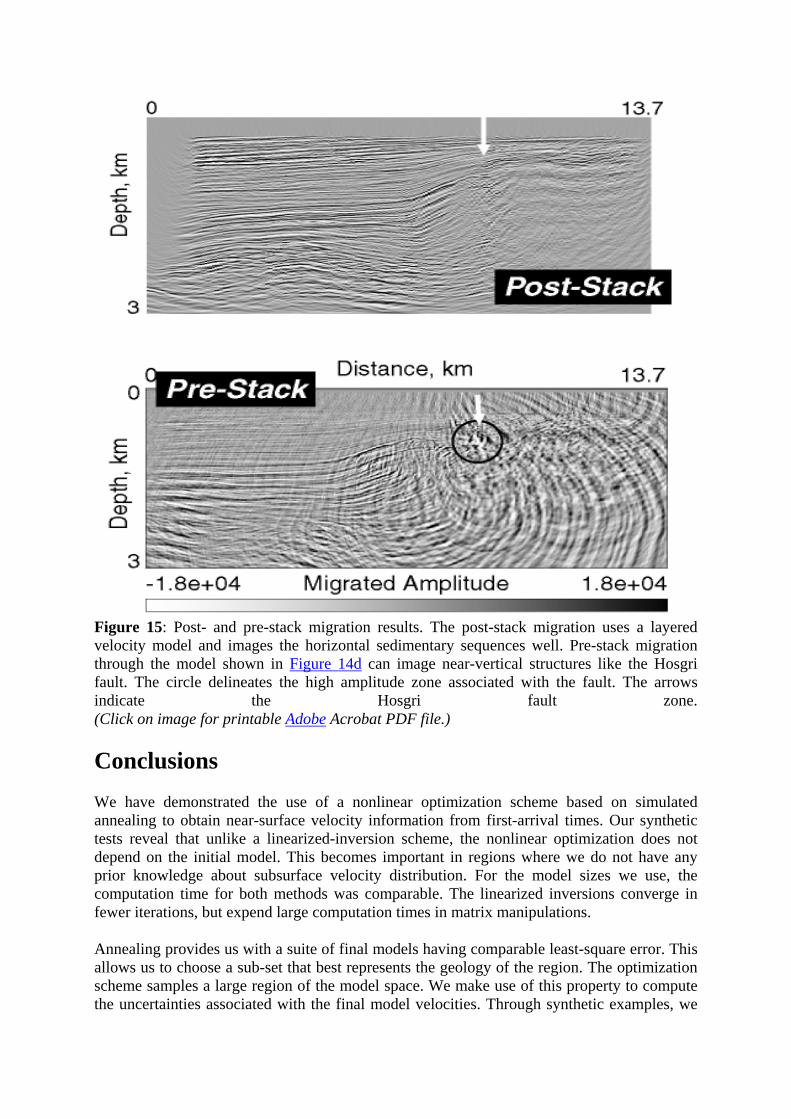
Figure 15: Post- and pre-stack migration results. The post-stack migration uses a layered velocity model and images the horizontal sedimentary sequences well. Pre-stack migration through the model shown in Figure 14d can image near-vertical structures like the Hosgri fault. The circle delineates the high amplitude zone associated with the fault. The arrows indicate the Hosgri fault zone. (Click on image for printable Adobe Acrobat PDF file.)

Conclusions

We have demonstrated the use of a nonlinear optimization scheme based on simulated annealing to obtain near-surface velocity information from first-arrival times. Our synthetic tests reveal that unlike a linearized-inversion scheme, the nonlinear optimization does not depend on the initial model. This becomes important in regions where we do not have any prior knowledge about subsurface velocity distribution. For the model sizes we use, the computation time for both methods was comparable. The linearized inversions converge in fewer iterations, but expend large computation times in matrix manipulations.

Annealing provides us with a suite of final models having comparable least-square error. This allows us to choose a sub-set that best represents the geology of the region. The optimization scheme samples a large region of the model space. We make use of this property to compute the uncertainties associated with the final model velocities. Through synthetic examples, we

show that the normalized deviations we obtain do indeed correspond to the normalized absolute difference between a ``true'' model and the optimization result. In addition we trace rays through our results to separate regions that are well constrained from regions that are not.

The first-arrival optimization has several applications. We present two such uses. Obtaining shallow-crustal velocities can be important for understanding the tectonic behavior of a region. We use data collected by COCORP to image the shallow-crustal velocities in the extended domain of the Death Valley region of California. Near-surface velocities are also important for doing residual statics corrections in reflection data processing. We show the robustness of the models obtained by annealing by computing vertical travel times through them. Finally, we use the velocity model obtained from first-arrival picks to carry out a pre-stack Kirchhoff migration. This is done to image in cross-section the Hosgri fault, which lies in a region of strong lateral velocity changes. The successful imaging of the fault demonstrates the ability of the generalized simulated annealing to produce accurate velocity images of the subsurface from first-arrival picks.

Acknowledgements

The COCORP Death Valley data were graciously provided by Sid Kauffman, Larry Brown and Steve Gallow of Cornell University. The data from the EDGE RU-3 line used in this study were provided by Anne Meltzer of Lehigh University and Don Reed of the Univ. ofCalifornia, Santa Cruz. This research was supported by the National Science Foundation under grant EAR-9296125 and by the U.S. Geological Survey under contract number 1434-92-6-2176. The authors would like to thank the Associate Editor John Vidale, and Mrinal Sen for their helpful reviews and suggestions.

References Ammon, C. J. and J. E. Vidale (1993). Tomography without rays, Bulletin of the Seismological Society of America, 83, 509-528.

Basu, A. and L. N. Frazer (1990). Rapid determination of critical temperature in simulated annealing inversion, Science, 249, 1409-1412.

Bohachevsky, I. O., M. E. Johnson, and M. L. Stein (1986). Generalized simulated annealing for function optimization, Technometrics, 28, 209-217.

Clayton, R. W. and G. A. McMechan (1981). Inversion of refraction data by wave field continuation, Geophysics, 46, 860-868.

Crouch, J. K., S. B. Bachman, and J. T. Shay (1984). Post-Miocene compressional tectonics along the central California margin, in Tectonics and Sedimentation Along the California Margin, J. K. Crouch and S. B. Bachman (Editors), Vol. 38, Pacific Section, Society of Economic Paleontologists and Mineralogists, San Diego, 37-54.

de Amorim, W. N., P. Hubral, and M. Tygel (1987). Computing field statics with the help of seismic tomography, Geophysical Prospecting, 35, 907-919.

DiSilvestro, L. A., K. H. Hanson, W. R. Lettis, and G. I. Shiller (1990). The San Simeon/Hosgri pull-apart basin, south-central coastal California (abstract), EOS Transactions of the American Geophysical Union, 71, 1632.

Docherty, P. (1992). Solving for the thickness and velocity of the weathering layer using a 2-D refraction tomography, Geophysics, 57, 1307-1318.

Farrell, R. C. and R. N. Euwema (1984). Refraction statics, Proceedings of IEEE, 72, 1316-1329.

Fawcett, J. A. and R. W. Clayton (1984). Tomographic reconstruction of velocity anomalies, Bulletin of the Seismological Society of America, 74, 2201-2219.

Geist, E. L. and T. M. Brocher (1987). Geometry and subsurface lithology of southern Death Valley basin, California, based on refraction analysis of multichannel seismic data, Geology, 15, 1159-1162.

Gerver, M. L. and V. Markushevitch (1966). Determination of a seismic wave velocity from the travel time curve, Geophysical Journal of the Royal Astronomical Society, 11, 165-173.

Graham, S. A. and W. R. Dickinson (1978). Evidence for 115 km of right slip on the San Gregorio - Hosgri fault trend, Science, 199, 179-181.

Haeni, F. P. (1986). Application of seismic refraction methods in groundwater modeling studies in New England, Geophysics, 51, 236-249.

Hagedoorn, J. G. (1959). The plus-minus method of interpreting seismic refraction sections, Geophysical Prospecting, 7, 158-182.

Hall, C. A. (1975). San Simeon - Hosgri fault system, coastal California: Economic and environmental implications, Science, 190, 1291-1294.

Hatherly, P. J. and M. J. Neville (1986). Experience with the generalized reciprocal method of seismic refraction interpretation for shallow engineering site investigation, Geophysics, 51, 255-265.

Hampson, D. and B. Russell (1984). First-break interpretation using generalized linear inversion, Journal of the Canadian Society of Exploration Geophysicisits, 20, 40-54.

Hanson, K. L. and W. R. Lettis (1990). Use of ratios of horizontal to vertical components of slip to asses style of faulting Hosgri fault zone, California (abstract), EOS Transactions of the American Geophysical Union, 71, 1632.

Honjas, William J. (1993). Results of post- and pre-stack migrations: imaging the Hosgri fault, offshore Santa Maria basin, CA, M.S. thesis, Univ. of Nevada-Reno, Reno.

Honjas, B., Louie, J., and Pullammanappallil, S., 1992, Results of post and pre-stack migrations imaging the Hosgri fault, offshore Santa Maria basin, CA (abstract), EOS Transctons of the American Geophysical Union, 73, supplement to no. 43 (Oct. 27), p. 390.

Jackson, D. D. (1972). Interpretation of inaccurate, insufficient, and inconsistent data, Geophysical Journal of the Royal Astronomical Society, 28, 97-109.

Jones, G. M. and D. B. Jovanovich (1985). A ray inversion method for refraction analysis, Geophysics, 50, 1701-1720.

Landa, E., W. Beydoun, and A. Tarantola (1989). Reference velocity model estimation from prestack waveforms: coherency optimization by simulated annealing, Geophysics, 54, 984-990.

Lees, J. M. and R. S. Crosson (1989). Tomographic inversion for three-dimensional velocity structure at Mount St. Helens using earthquake data, Journal of Geophysical Research, 94, 5716-5728.

Louie, J. N., R. W. Clayton, and R. J. LeBras (1988). Three-dimensional imaging of steeply dipping structure near the San Andreas fault, Parkfield, California, Geophysics, 53, no. 2, 176-185.

Louie, J. N. and J. Qin (1991). Structural imaging of the Garlock fault, Cantil Valley, California, Journal of Geophysical Research, 96, 14,461-14,479.

Louie, J. N., Pullammanappallil, S. K., and W. Honjas (1997). Velocity Models for the highly extended crust of Death Valley, California, Geophysical Research Letters, 24, 735-738.

McIntosh, K. D., D. L. Reed, E. A. Silver, and A. S. Meltzer (1991). Deep structure and structural inversion along the central California continental margin from EDGE seismic profile RU-3, Journal of Geophysical Research, 96, 6459-6473.

McMechan, G. A., R. W. Clayton, and W. D. Mooney (1982). Application of wave field continuation to the inversion of refraction data, Journal of Geophysical Research, 87, 927-935.

Metropolis, N., A. Rosenbluth, M. Rosenbluth, A. Teller, and E. Teller (1953). Equation of state calculations by fast computing machines, Journal of Chem. Phys., 21, 1087-1092.

Namson, J. and T. L. Davis (1990). Late Cenozoic fold and thrust belt of the southern Coast Ranges and Santa Maria Basin, California, Bulletin of the American Association of Petroleum Geologists, 74, 467-492.

Olsen, K. B. (1989). A stable and flexible procedure for the inverse modeling of seismic first arrivals, Geophysical Prospecting, 37, 455-465.

Palmer, D. (1981). An introduction to the generalized reciprocal method of seismic refraction interpretation, Geophysics, 46, 1508-1518.

Pullammanappallil, S. K. and J. N. Louie (1993). Inversion of seismic reflection traveltimes using a nonlinear optimization scheme, Geophysics, 58, 1607-1620.

Rockwell, D. W. (1967). A general wavefront method, in Seismic Refraction Prospecting, A. W. Musgrav (Editor), Society of Exploration Geophysicists, Tulsa, Oklahoma, 363-415.

Rothman, D. H. (1985). Non-linear inversion, statistical mechanics, and residual statics estimation, Geophysics, 50, 2797-2807.

Rothman, D. H. (1986). Automatic estimation of large residual statics corrections, Geophysics, 51, 332-346.

Russell, B. H. (1989). Statics corrections - a tutorial, Canadian Society of Exploration Geophysicsits Recorder, 16-30.

Sen, M. K. and P. L. Stoffa (1991). Nonlinear one-dimensional seismic waveform inversion using simulated annealing, Geophysics, 56, 1624-1638.

Shaw, P. R. and J. A. Orcutt (1985). Waveform inversion of seismic refraction data and applications to young Pacific crust, Geophysical Journal of the Royal Astronomical Society, 82, 375-414.

Simmons, Jr., J. L. and M. M. Backus (1992). Linearized tomographic inversion of first-arrival times, Geophysics, 57, 1482-1492.

Stewart, J. H. (1971). Basin and Range structure: a system of horsts and grabens produced by deep-seated extension, Geological Society of America Bulletin, 82, 1019-1044.

Thornburgh, H. R. (1930). Wavefront diagrams in seismic interpretation, Bulletin of the American Association of Petroleum Geologists, 14, 185-200.

Vasudevan, K., W. G. Wilson, and W. G. Laidlaw (1991). Simulated annealing static computation using an order-based energy function, Geophysics, 56, 1831-1839.

Vidale, J. E. (1988). Finite difference calculation of travel times, Bulletin of the Seismological Society of America, 78, 2062-2076.

Wernicke, B. (1992). Cenozoic extensional tectonics of the U.S. Cordillera, in The Cordilleran Orogen; Conterminous United States, B. C. Burchfield, P. W. Lipman, and M. L. Zoback (Editors), Geological Society of America, Boulder, 553-581.

Wernicke, B., G. J. Axen, and J. K. Snow (1988). Basin and range extensional tectonics at the latitude of Las Vegas, Nevada, Geological Society of America Bulletin, 100, 1738-1757.

Wiggins, R. (1972). The general inverse problem: implication of surface waves and free oscillations on Earth structure, Review of Geophysics and Space Physics, 10, 251-285.

Wright, L. A. (1976). Late Cenozoic fault patterns and stress fields in the Great Basin and westward displacement of the Sierra Nevada block, Geology, 4, 489-494.