a generative system for shape configuration - code...
TRANSCRIPT

ArchiDNA:
A Generative System for Shape Configuration
Doo Young Kwon
A thesis submitted in partial fulfillment of the requirements for the degree of
Master of Science in Architecture
University of Washington
2003
Program Authorized to Offer Degree: Architecture


University of Washington
Graduate School
This is to certify that I have examined this copy of a master’s thesis by
Doo Young Kwon
and have found that it is complete and satisfactory in all respects,
and that any and all revisions required by the final
examining committee have been made.


In presenting this thesis in partial fulfillment of the requirements for a Master’s degree
at the University of Washington, I agree that the Library shall make its copies freely
available for inspection. I further agree that extensive copying of this thesis is allowable
only for scholarly purposes, consistent with “fair use” as prescribed in the U.S.
Copyright Law. Any other reproduction for any purposes or by any means shall not be
allowed without my written permission.


University of Washington
Abstract
ArchiDNA:
A Generative System for Shape Configuration
Doo Young Kwon
Chair of the Supervisory Committee:
Professor Ellen Yi-Luen Do
Department of Architecture
This thesis concerns a new generation process for shape configurations using a set of operations.
The approach derives from analyzing a particular design style and programming them into a
computer. It discusses how generative CAD software can be developed that embodies a style
and how this software can serve in the architectural design process as a computational design
tool.
The thesis proposes a prototype software system, ArchiDNA, to demonstrate the use of
operations to generate drawings in a specific design style. ArchiDNA employs a set of
operations to produce design drawings of shape configuration in Peter Eisenman's style for the
Biocentrum building plan in Frankfurt, Germany. The principles of form generation are defined
as a set of operations. ArchiDNA generates 2D and 3D drawings similar to Eisenmans plan and
model for the Biocentrum building.
The extension system of ArchiDNA, called ArchiDNA++, supports designers in defining
operations and generating shape configurations. Designers can enter and edit their own shapes
for the generation process and also control the parameters and attributes for shape operations.
Thus, designers can manage the generation process and explore using ArchiDNA++, to generate
shape configurations that are consistent with their own drawing style.


Table of Contents
List of Figures .............................................................................................................................. iv
Chapter One: Architectural Drawing and Analysis of Style
1. Introduction ............................................................................................................................... 1
1.1. Role of Architectural Drawing........................................................................................... 1 1.1.1. A Generative Device to Find a Building Form........................................................... 1 1.1.2. Computer Generated Drawing.................................................................................... 2 1.1.3. Generative Drawing Machine..................................................................................... 3
1.2. Style Analysis .................................................................................................................... 5 1.2.1. What is Design Style?................................................................................................. 5 1.2.2. Style Analysis in a Drawing ....................................................................................... 5 1.2.3. Style Analysis with a Computer ................................................................................. 6
1.3. The Goal of the Thesis ....................................................................................................... 7
1.4. Outline of the Thesis .......................................................................................................... 8
Chapter Two: Analysis of Style and Generative Systems
2. Related Work............................................................................................................................. 9
2.1. Analysis of Style ................................................................................................................ 9 2.1.1. Shape Grammar .......................................................................................................... 9 2.1.2. Analysis and Generation of Style with Shape Grammar .......................................... 13 2.1.3. Analysis and Generation of Style with Other Algorithmic Approaches................... 21
2.2. Generative Applications................................................................................................... 23 2.2.1. Shape Grammar Interpreters..................................................................................... 23 2.2.2. Algorithmic Shape or Form Generation ................................................................... 26
2.3. Discussion ........................................................................................................................ 30
i
Chapter Three: An Eisenman Design Machine
3. ArchiDNA............................................................................................................................... 31
3.1. Eisenman’s Biocentrum Building Design ....................................................................... 31
3.2. 2-D Operations ................................................................................................................ 33 3.2.1. Primitive Operations in ArchiDNA.......................................................................... 33 3.2.2. Application Process: applier-shape and base-shape ................................................. 35
3.3. 2-D Generation ................................................................................................................ 37
3.4. 3-D Operatations.............................................................................................................. 39
3.5. 3-D Generation ................................................................................................................ 40
3.6. Summary.......................................................................................................................... 41
3.7. Discussion........................................................................................................................ 41
Chapter Four: An End-User Programming Environment For Shape Configuration
4. ArchiDNA ++ ......................................................................................................................... 43
4.1. ArchiDNA++ Environment ............................................................................................. 44 4.1.1. Tool Palette .............................................................................................................. 44 4.1.2. Drawing Window ..................................................................................................... 45 4.1.3. Four Control Palettes................................................................................................ 45
4.2. ArchiDNA++ in use ........................................................................................................ 46
4.3. Shape Preparation Phase.................................................................................................. 47 4.3.1. Shape Creation ......................................................................................................... 47 4.3.2. Shape Attribute Control ........................................................................................... 48
4.4. Shape Configuration Phase.............................................................................................. 51 4.4.1. Define applier-shape(s) ............................................................................................ 51 4.4.2. Select base-shape or Draw base-shape..................................................................... 51
4.5. 3-D Conversion................................................................................................................ 52 4.5.1. Threshold Setting ..................................................................................................... 53 4.5.2. 3D Mode Setting ...................................................................................................... 53
4.6. Example: Generation of a Sunflower Shape.................................................................... 54 4.6.1. Shape Preparation..................................................................................................... 55 4.6.2. Shape Configuration................................................................................................. 56
ii

Chapter Five: Implementation of ArchiDNA++
5. Implementation........................................................................................................................ 59
5.1. System Architecture......................................................................................................... 59
5.2. Shape Data Structure........................................................................................................ 60
5.3. Shape Configuration ........................................................................................................ 61
5.4. Exporting VRML Models ................................................................................................ 62
5.5. Discussion ........................................................................................................................ 63
Chapter Six: Future Work and Conclusion
6. Future Work and Conclusion .................................................................................................. 64
6.1. Future Work ..................................................................................................................... 64 6.1.1. Spatial Configurations .............................................................................................. 64 6.1.2. ArchiDNA as a Kind of Shape Grammar ................................................................. 66 6.1.3. 3D Form Configuration ............................................................................................ 67
6.2. Conclusion ....................................................................................................................... 68
Bibliography................................................................................................................................ 70
iii

List of Figures
Figure Number Page
1.1. Drawings for Peter Eisenman’s House Project (Eisenman, 1975).
Source: Eisenman, 1987 ......................................................................................................... 2
1.2. Computer generated drawings for Eisenman’s Groningen Video Pavilion Project
(Eisenman, 1990). Source: Eisenman, 1996........................................................................... 3
2.1. (a) Rules for a Standard Shape Grammar (b) A derivation of the rules
(c) A result generated by applying the rules repeatedly. Source: Stiny, 1985...................... 10
2.2. (a) Rules for a Parametric Shape Grammar (b) A derivation of the rules
(c) A result shapes generated by applying the rules. Source: Stiny, 1985............................ 11
2.3. Various 2D labeled rules for standard shape grammar and their derivations.
Source: Knight, 2001............................................................................................................ 12
2.4. Various 3D labeled rules for standard shape grammar and their derivations.
Source: Knight, 2001............................................................................................................ 12
2.5. (a) Some results of ice-ray grammar (b) Four rules for a shape grammar of an ice-ray
pattern. Source: Stiny, 1977 ................................................................................................. 14
2.6. A derivation using the third and fourth rule of ice-ray grammar. Source: Stiny, 1977 ....... 14
2.7. Possible Palladian villa plans with Palladian villas grammar.
Source: Stiny and Mitchell, 1978 ......................................................................................... 15
2.8. A derivation of Villa Malcontenta using Palladian viallas grammar.
Source: Mitchell, 1994 ......................................................................................................... 16
2.9. (a) A massing rule (b) Detailing rules for the prairie house grammar.
(c) A derivation of the rules. Source: Koning and Eizenberg, 1985..................................... 17
2.10. Various results of the prairie house grammar. Source: Koning and Eizenberg, 1985 ....... 18
2.11. A part of the rules for a Diebenkorn Ocean Park Grammar.
Source: Kirsch and Kirsch, 1986.......................................................................................... 19
2.12. Steps in the generation of Diebenkorn’s Ocean Park No. 111 from the grammar.
Source: Kirsch and Kirsch, 1986.......................................................................................... 19
2.13. (a) Generation rules for wall architecture (b) Configurations generated by these rules.
iv

Source: Flemming, 1990....................................................................................................... 20
2.14. (a) Snapshot of a program, “Make Anthropomorph Shape” (b) Various anthropomorphic
shapes generated by the program. Source: Kirsch and Kirsch, 1998.................................... 21
2.15. (a) Prepared shapes from analyzing Miro’s painting (b) A final Miro composition
generated by using the prepared shapes. Source: Kirsch and Kirsch, 1998.......................... 22
2.16. Generation of a Palladian villa in PlanMaker system
Source: Hersey and Freedman, 1992 .................................................................................... 23
2.17. Possible Palladian villa plans generated in PlanMaker system
Source: Hersey and Freedman, 1992 .................................................................................... 23
2.18. Screenshot of GEdit Interface. Source: Tapia, 1999 .......................................................... 24
2.19. Screenshot of Shaper 2D Interface. Source: Mcgill, 2000 ................................................. 24
2.20. Illustrations for using the result of Shaper2D in the design process (a) The generated
result in Shaper 2D (b) Site planning with the result (c) Plan designing with the result.
Source: Mcgill, 2000 ............................................................................................................ 25
2.21. (a) Screenshot of 3D Shaper Interface (b) Screenshot of SGI Open Inventor Viewer
to see the 3D result of 3D Shaper. Source: Wang, 1999....................................................... 25
2.22. The turtle commands to generate shape configuration in Logo Programming
Environment. Source: http://el.media.mit.edu/logo-foundation/ ......................................... 27
2.23. Snapshot of Design by Number Interface. Source: http://dbn.media.mit.edu/................... 27
2.24. Various Results of Design by Number. Source: http://dbn.media.mit.edu/ ....................... 28
2.25. Snapshot of FormWriter Interface. Source: Gross, 2001 ................................................... 28
2.26. Models of historic Islamic structures by students using the FormWriter
Source: Gross, 2001.............................................................................................................. 29
2.27. Snapshot of Processing Working Environment. Source: http://www.proce55ing.net/ ...... 30
3.1. (a) Biocentrum (Eisenman, 1996) (b) Diagram of DNA showing Amino Acids
(c) Four distinct shapes in Amino Acids. Source: Eisenman, 1999 ..................................... 32
3.2. Drawings for Biocentrum (Eisenman, 1996) (a) Plan (b) Axonometric View.
Source: Eisenman, 1999 ....................................................................................................... 33
3.3. Primitive Shape Operations.................................................................................................. 34
3.4. A square is attached to a line considering its location, angle, and size ................................ 34
3.5. Square is attached to four edges of the first square. ............................................................. 35
v

3.6. Four Shape Operations with applier-shape to base-shape.................................................... 36
3.7. Four shapes (A1-A2-A3-A4) applied sequentially to the edges of the base-shape B. Note
that shape A1 occurs twice because the application process repeats at the beginning once
the sequence is exhausted..................................................................................................... 36
3.8. Initial shape in ArchiDNA Interface.................................................................................... 37
3.9. (a) Application the applier-shape G (ribbon) to the base-shape C (pentagon)
(b) Application the applier-shape G to the base-shape A (arch) .......................................... 37
3.10. ArchiDNA Second Shape Generation................................................................................ 38
3.11. 2D Eisenman-like drawing generated in ArchiDNA ......................................................... 39
3.12. 3D form generation in ArchiDNA (a) Calculating the area of two applied shapes A1&A2
and assigning heights (b) Comparing areas with a threshold and deciding up and down (c)
Extrusion of small shape A1 upward and extrusion of large shape A2 downward (d)
Extrusion of shape B with a user-defined height.................................................................. 40
3.13. 3D Eisenman-like Model Generated in ArchiDNA........................................................... 40
3.14. Four steps of process to generate Eisenman-like drawing ................................................. 41
4.1. Snapshot of ArchiDNA++ Interface .................................................................................... 45
4.2. Four Control Palettes ........................................................................................................... 46
4.3. Overview of ArchiDNA++ Operation ................................................................................. 47
4.4. Created Shapes – left: attributes of a rectangle shape, and a small red-rectangle label
(¬) in the center of an edge marks an anchor-edge (for lines and poly-lines)...................... 48
4.5. Changing anchor-edge of applier-shape object (ribbon) and the result of applying it to a
base-shape object (pentagon); dotted lines illustrates the default configuration that uses
anchor-edge at the top of ribbon........................................................................................... 49
4.6. Change two attachable-edges of base-shape object (pentagon) to un-attachable edges
and its result with an applier-shape object (ribbon). ............................................................ 49
4.7. Fix three edges with angle (90°) and scale-factor (50%) and its result shows
three applier-shape objects are not matched to the base-shape object.................................. 50
4.8. (a) Counter-clockwise base-shape object (b) Clockwise base-shape object
with four applier-shape objects (A1-A2-A3-A4) ................................................................. 51
4.9. Various Shape Configurations in ArchiDNA++.................................................................. 52
4.10. 3D Mode: block-mode and wall-mode (a) 3D model generated in block-mode
vi

(b) 3D model generated in wall-mode. ................................................................................. 53
4.11. (a) ArchiDNA++ 3D Model in VRML Viewer, Cortona (b)ArchiDNA++ 3D Model
imported into formZ. ............................................................................................................ 54
4.12. (a) First sketch drawing for generating a sunf1ower shape (b) Second sketch drawing
for elaborating the first sunflower shape .............................................................................. 54
4.13. Create three shapes (ribbon, triangle, and hexagon) .......................................................... 55
4.14. Change shape attributes (attachable-edge and anchor-edge).............................................. 56
4.15. (a) First shape configuration for sunflower-like shape attaching ribbons to a pentagon (b)
Second shape configuration for sunflower-like shape attaching a triangle to the ribbon
base-shape objects ................................................................................................................ 54
5.1. ArchiDNA++ System Architecture. ..................................................................................... 59
5.2. Representation of a ribbon-like shape with points and edges (a) five points with 2D
coordinates (b) five edges with anchor-edge mark [*], attachable-edge mark [+], un-
attachable-edge mark [-], and operation values [angle and scale] (c) the final display
on the screen. ........................................................................................................................ 60
5.3. Data Structure for a ribbon-like shape in ArchiDNA........................................................... 61
5.4. A System Diagram for the Process of Shape Configuration ................................................ 62
5.5. Converting a 2D shape (ribbon) to 3D VRML objects. ....................................................... 63
6.1. Representation of a ribbon space.......................................................................................... 65
6.2. Data structure for a ribbon space.......................................................................................... 65
6.3. 3D conversion of a ribbon space .......................................................................................... 65
6.4. Rules for a grammar of ArchiDNA application process ...................................................... 66
6.5. Optional Rules for a grammar of ArchiDNA application process ....................................... 67
6.6. 3D form configuration of applying 3D applier-shape to 3D base-shape.............................. 68
vii

Acknowledgements
I am grateful to several people for their support and advice especially my three advisors,
professors Ellen Yi-Luen Do, Mark D. Gross and Brian R. Johnson. I am also thankful for the
thoughtful comments and suggestions of my colleagues in the Design Machine Group: Ken
Camarata, Karen Hanson, Mike Weller, Chen-Je Huang, Markus Eng, Yeon Joo Oh, and Eun
Soo Lee. I will never forget their energetic collaboration in Design Computing Research.
Especially, I thank Ken Camarata and Karen Hanson for their beautiful comments on my
English and my life in Seattle.
I also want to deeply thank my college professor, Jin Won Choi, for introducing me to the field
of Design Computing and the way to be a good programmer.
This wouldn’t have been possible without the love and support from my parents, Tae Eung
Kwon and Ho Nam Choi; my brother, Doo Hyoun Kwon; my sister, Nam Hee Kwon; and my
love, Moon Sun Jung.
An extra special thanks to Ellen Do and Mark Gross for their dedication and assistance in my
research life.
This research was supported in part by the National Science Foundation under CCLI-EMD
Grant DUE-0127579. The views and findings contained in this material are those of the author
and do not necessarily reflect the views of the National Science Foundation.
viii

1
Chapter One
Architectural Drawing and Analysis of Style
1. Introduction
1.1. ROLE OF ARCHITECTURAL DRAWING
1.1.1. A Generative Device to Find a Building Form
Designers often draw shapes to investigate building forms in the schematic design process.
Architectural educator, Herbert (1993) argues that “study drawings” is a medium for designers
to find formal design ideas. He states that the important characteristic of a study drawing is its
graphic ambiguity. Unlike final plan drawings with details and specifications, study drawings
provide a variety and fluid formal design ideas to the designer. Thus this kind of drawing is
useful for designers to explore a building form in a schematic design process. The ambiguity of
drawing may be obtained with irregular overlays of various colors, in shapes, spaces, lines, or in
images with any specified degree of irregularity. Fraser and Henmi (1993) also argue the
importance of ambiguity and irregularity in drawings. Architects use drawings to find design
ideas. They draw shapes from their minds’ eye or preconceived images. Then the designers
develop a drawing further by combining these previously generated shapes. This process is
repeated until the drawing becomes closer to the designer’s preconceived images. Through this
repetitive generation process, the designer finds or develops a formal design idea.
Peter Eisenman, a contemporary American architect made a specific statement about drawings
as a generative device. He stated that “What I do is set up a series of ideas or rules or strategies
and draw into those, trying to find some form in those ideas (quoted in Herbert, 1993).” He uses
drawing in his design process to find the relationship of the formal to the conceptual. He
intentionally manipulates and utilizes the effects of drawing to explore design problem

2
(Eisenman, 1999). Eisenman uses drawing to search for a form and idea and explains how the
form and idea can be manipulated. Figure 1.1 shows a set of drawings from Peter Eisenman’s
House project. He repeatedly adds lines to the previous drawings and develops a plan of the
house from left to right. He transforms portions of the design and draws more details. This
series of drawings illustrate how he uses drawings as a generative device to explore formal
design idea.
Figure 1.1: Drawings for Peter Eisenman’s House Project (Eisenman, 1975)
Source: Eisenman, 1987
1.1.2. Computer Generated Drawing
Architects are increasingly using computers to generate 2D and 3D drawings in the design
process. They use a computer not only to represent the final product but also to explore
architectural form during the schematic phase of design. Kolarevic (2000) surveys some
different approaches in which architects use the computer to find a building form in
contemporary architectural design. He called these approaches digital architectures (Kolarevic,
2000). Various computer software systems are used to manipulate or generate forms for
architectural design. For example, Greg Lynn (1999) uses animation software to generate
building form. He visualizes his design concept with animated 3D objects to develop an
architectural form.
Peter Eisenman is also widely considered as a designer of digital architecture (Kolarevic, 2000).
He believes the computer-generated drawings are useful for exploring building form

3
possibilities [Galofaro, 1999]. He uses computer algorithms to generate drawings for formal
design idea in design process. Figure 1.2 shows computer-generated drawings for Eisenman’s
Groningen Video Pavilion (Eisenman, 1996). Different from his House project drawings [Fig.
1.1], he uses simple CAD functions (copy, translation, and rotation) which manipulate shapes.
Instead of drawing with a pen, he used those operations using a mouse in a CAD system. This
computer drawing process is also repeated to generate a series of alternative drawings [Fig. 1.2].
Figure 1.2: Computer generated drawings for Eisenman’s Groningen Video Pavilion Project (Eisenman,
1990). Source: Eisenman, 1996
1.1.3. Generative Drawing Machine
We saw in the previous sections that architects generate drawings to explore design ideas about
form. They use a conventional drawing tool (pen and paper) or a CAD program. Regardless of
drawing medium, they represent and develop a visual idea repeatedly until they find a building
form. Therefore we believe that a design tool that allows designers to quickly create drawing
alternatives might be useful. Even though current CAD software supports the creation of basic
drawings, it is not easy to learn and control these operations. Even if a designer already knows
how to operate CAD system, it can be time consuming and labor-intensive to produce proposed
drawings that support a formal design idea. This is one reason why many designers use a
computer only to present a final product, but not in the early and creative phases of design.
Computers can be useful for a designer to get results in an effective way. A computer can be
programmed to generate various drawing results from a designer’s simple input. Therefore,
various research efforts such as shape grammars and algorithmic shape generation have

4
explored this approach (Flemming, 1990; Gross, 2001). They describe how a computer can
algorithmically generate multiple formal ideas in an early design phase.
These generative systems are based on the basic concept of computation: input information is
transformed or operated on in some functions to produce output. A computer follows an
algorithm produce with the input. Using the concept of computation, a generative drawing
machine can be developed with shape manipulation algorithms. When a designer inputs certain
shapes, the computer generates shape configurations following the algorithms defined by the
designer. A designer can then generate different shape configurations by repeating this
generation process. This generation process is similar to Eisenman’s drawing method, which
sets up “a series of ideas or rules or strategies” and draws from them, “to find some form in
those ideas. (Eisenman, 1999)”
The common goal of generative systems is to generate drawings using computer algorithms. In
other words, a designer uses this system to investigate formal design idea and explain the
generated form with the computer algorithms. The designer eventually uses the algorithms as a
design tool to create building form.
This thesis investigates two issues: to define algorithms for shape generation and to allow a
designer to easily control the generation process. Shape generation algorithms can be developed
for designers to create complicated shape patterns or to manipulate existing shapes. Moreover,
the algorithms can be embedded with a “design knowledge” that controls the shape generation
or manipulation. Drawing is a result of thinking in the design process. Therefore a drawing
machine should provide an interface for designers to think about design idea by controlling and
manipulating generation algorithms.

5
1.2. STYLE ANALYSIS
1.2.1. What is Design Style?
Style has been explained in several ways. Gombrich (1960) and Simon (1975) defined style as a
way of doing things. A style is produced when people select or produce a particular alternative
or process to find a solution. Style usually expresses characteristics of an individual or a group
of people for particular ways of thinking and doing things.
Design style is a kind of design knowledge that characterizes a particular artifact or a group of
design work (Shapiro, 1961). A design style can be described as consisting of certain elements
and ways to compose those elements. For example, when we look at architectural drawings or
buildings, we can recognize their forms and qualities as displaying a certain style such as the
pointed arch for Gothic and Islamic architecture, the round arch for Roman and Byzantine.
Formal properties such as shape, color, arrangement, texture, size, and orientation are visual
elements of a style. In another words, a design style means that the features of an object as well
as the relationships between the components of the object can be recognized explicitly.
Therefore a style can be described in terms of the common components of a design and how
they are arranged.
Many architecture schools teach various design styles in the design. Studio students develop
design knowledge by imitating other design styles. They learn to create and manipulate design
elements by studying the other designs. It can help a designer to understand the style.
Eventually, the designer can apply the understanding of the style to his or her own design.
1.2.2. Style Analysis in a Drawing
The design style of architectural drawings can be analyzed by the identifying drawing elements
and their relationships. Architectural drawings usually represent architectural components such
as walls, doors, columns, rooms, and so on. These components are used as formal elements to
6
analyze architectural drawings. For example, Stiny and Mitchell analyzed the plans of Palladian
villas to define how architectural components can be generated or arranged to create floor plans
in the style of the Palladian villas.
However, some drawing types (study drawings or design drawings) do not exactly represent
architectural components. Architects use these drawings as a visual tool to find a building form
in a schematic design process. These drawings might have form elements such as patterns and
shapes. Using the form elements, a style of the drawing can be analyzed and described. For
example, Stiny (1972) describes a stylistic pattern of the Chinese lattice window as a set of rules.
Kirsch and Kirsch (1986) analyzed and described a style for Richard Diebenkorn’s abstract
paintings. Even though these are not architectural drawings, they show that a style can be
defined as consisting of elements and spatial relationships. Likewise, style in architectural
drawings can be represented by a set of shapes and their relationships. The shapes can be
recognized visually from the drawing. The spatial relationships can be represented with basic
transformations (translation, rotation, and scaling) in a Cartesian coordinate system.
1.2.3. Style Analysis with a Computer
As explained in the previous section, a design style is a kind of design knowledge that can be
learned and then used in design process. We recognize a design style in the formal properties of
a drawing. The advance of computer technology helps us to analyze a design style in different
way. For example, a design style in a drawing is studied in the form of computer algorithms that
manipulate the design components (Kirsch, 1998). Char and Gero (1999) identified common
shapes in a set of architectural drawings that belongs to a design style. They used basic
transformations of computer graphics such as translation, rotation, scaling, and mirroring to
represent the shapes and the relations. The purpose of these studies is to support a designer to
understand and learn a design style and then develop his or her own style using a computer.
Since Stiny and Gips introduced shape grammar to explore the idea of using a set of rules to
represent a painting (Stiny & Gips, 1972), many shape grammar systems have demonstrated
how a computer can generate shapes with certain graphic or architectural styles. Much work in
7
shape grammar has analyzed specific design styles using a set of rules and then showed how
those rules can be used to generate new designs in that style (Knight, 2000). Separately from the
shape grammar have been the studies using computer graphic algorithms. For example, Kirsch
and Kirsch (1986) defined the style of the Spanish painter Joan Miro. They describe the
common shapes in Miros drawings with algorithms which can manipulate the shapes. Hersey
and Freedman (1992) also developed a ‘split’ algorithm that divide a square horizontally or
vertically for Palladian design style. This simple algorithm generates various building plans in
the Palladian style. These systems show how a design style can be defined in terms of a set of
algorithms and how a designer can develop a new design style or modify an existing style
systematically.
1.3. THE GOAL OF THE THESIS
This thesis examines how a generative CAD software program can be developed to embody a
style and how this program can serve as a computational tool in design. It discusses design style
in architectural drawing, a set of algorithms (or operations) to generate drawings in a design
style, and develop a generative system to exercise those algorithms. This thesis has two main
goals.
The first goal is to program a design style into a computer system. A design style is an
important kind of design knowledge. If a design style can be programmed, it can help a
designer to understand this particular design style with a generative system. It enables a
designer to easily investigate formal design idea by interacting with the system.
A design style can be defined in several ways. The thesis investigates a design style exhibited in
particular drawings. This thesis chose to start with a design style represented in Peter
Eisenman’s drawings for Biocentrum Building. The drawing is composed with common
drawing features of which the composition can be geometrically described. The idea is that if
we can develop an algorithmic process to generate the drawings, then we may conclude that the
algorithm is a description of the style and a computer enables designers to generate drawings of
the same style. This thesis proposes a generative system, ArchiDNA to generate drawings of

8
Eisenman’s style. This system demonstrates that Eisenman’s style can be programmed as a set
of operations and how a designer can use it to make Eisenman-like drawings.
The second goal of the thesis is to generalize the algorithms initially defined for Eisenman’s
design style, and develops a generative system that enables designers to use and control the
generation process for their own design styles. For this, this thesis explores the development of
a system for designers to adapt the generation process of Eisenman-like drawing to their own
purposes. This approach can be seen as extension of a CAD program. The thesis describes an
easy-to-use generative system, ArchiDNA++. There are currently many CAD software
programs. However, it is still difficult for designers to learn the systems and use in the
schematic design process. ArchiDNA++ is a working system in which a designer can specify a
design style by describing a set of elements and combination to generate new drawings for
design in this way. The system allows a designer to investigate formal design ideas.
1.4. OUTLINE OF THE THESIS
The rest of this document is divided into six parts. Chapter Two describes related work,
including example applications of style analysis and generative systems for design. Chapter
Three describes ArchiDNA to demonstrate how one defines a certain design style with a set of
operations and generate drawings. Chapter Four explains the ArchiDNA++ software that allows
a designer to control the operations and generate drawings. Chapter Five explains the
computational implementation of the ArchiDNA++. Finally, Chapter Six concludes with a
discussion and identifies topics for future work.

9
Chapter Two
Analysis of Style and Generative Systems
2. Related Work
This chapter establishes the background and underlying principles for this thesis. This chapter
has two main sections. The first section reviews some computational approaches to the analysis
of style. The second section describes several generative systems for design.
2.1. ANALYSIS OF STYLE
2.1.1. Shape Grammar
Stiny introduced an idea of shape grammars to describe visual shape compositions (Stiny, 1985).
A shape grammar has a set of rules to specify how one shape or part of a shape can be replaced
by another. This simple substitution process is used to describe a certain design style. In other
words, a shape grammar defines a design style in the form of algorithms that manipulate the
design components. Several computer systems have demonstrated shape grammars to generate
shapes with a certain graphic or architectural style. Much work in shape grammar has analyzed
an instance of design style with a set of rules and showed how the rules can be used to generate
new designs in that style (Knight, 2000).
Stiny introduced two types of shape grammars: standard (non-parametric, basic, or standard)
shape grammars and parametric shape grammars (Stiny, 1985). Both have a set of rules [Fig.
2.1a]. In each rule, shape on the left side of the arrow determines which part of the shape will be
replaced when the rule is applied. The shape on the right side of the arrow indicates the state
after the transformation. An initial shape can be applied by a sequence of rules. Figure 2.1 b
shows how applying the same simple rule (#2) repeatedly generates a complex pattern.

10
Variation of how many iterations of applying the rule to the initial shape can generate an
interesting drawing [Fig. 2.1c].
(a)
(c)
(b)
Figure 2.1: (a) Rules for a Standard Shape Grammar (b) A derivation of the rules (c) A result generated
by applying the rules repeatedly. Source: Stiny, 1985
Like a standard shape grammar, a parametric shape grammar also has a set of rules that specify
how shapes replace sub-shapes of a composition [Fig. 2.2a]. However, it uses parameters for
shape manipulation. Shapes have proportion parameters, and the values of the parameters can
be changed. This parametric shape grammar creates shapes with more variation than the
standard shape grammar. Figure 2.2c shows the result of a parametric version of the shape
grammar shown in Figure 2.1c.

11
(a)
(c)
(b)
Figure 2.2: (a) Rules for a Parametric Shape Grammar (b) A derivation of the rules (c) A result shapes
generated by applying the rules. Source: Stiny, 1985
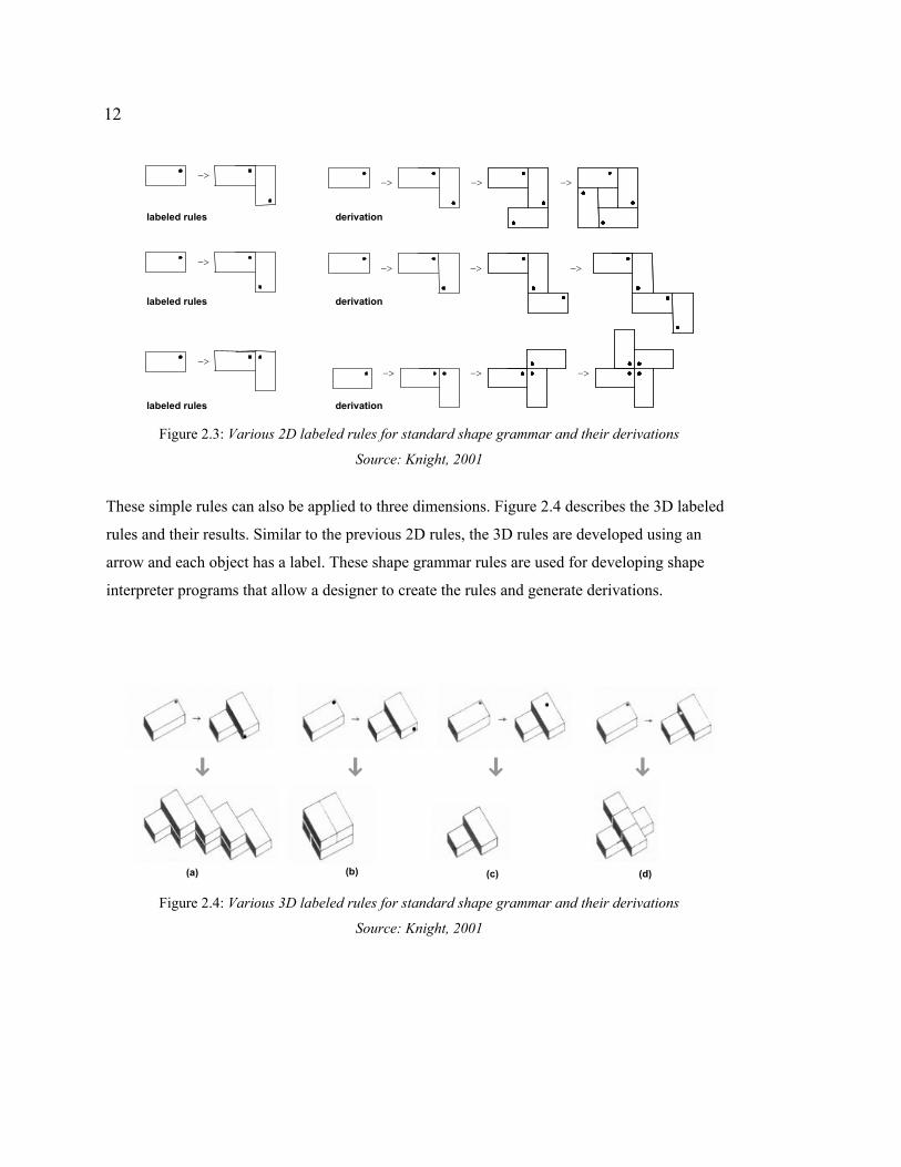
Changing a substitution rule of a shape grammar can generate various results. Figure 2.3 shows
three labeled rules and their derivations. A user arranges shapes using simple operations
(translation, rotation, scaling) and defines substitution rules. The label is a symbol that indicates
the orientation of the shape and how to apply this rule in a derivation. The labeled rules show
how a rectangle on the left side of the arrow would generate a copy of the shape in a spatial
argument. The two shapes on the right side of the arrow indicate the result of such rules. Left
hand side of the rule we have an initial shape with a dot label. Right hand side we have the
arranged shapes illustrating the derivation outcome. With labels at different position, each rule
generates a different derivation result.
12
−>−> −> −>
−>−> −> −>
−>−> −> −>
labeled rules derivation
labeled rules derivation
labeled rules derivation
Figure 2.3: Various 2D labeled rules for standard shape grammar and their derivations
Source: Knight, 2001
These simple rules can also be applied to three dimensions. Figure 2.4 describes the 3D labeled
rules and their results. Similar to the previous 2D rules, the 3D rules are developed using an
arrow and each object has a label. These shape grammar rules are used for developing shape
interpreter programs that allow a designer to create the rules and generate derivations.
(a) (b) (c) (d)
Figure 2.4: Various 3D labeled rules for standard shape grammar and their derivations
Source: Knight, 2001

13
Both standard and parametric shape grammars have been used for design style analysis and
applications. The next section shows how the parametric shape grammar has been used to
analyze design style. Then, this chapter also explains shape grammar interpreter-computer
based systems that generate 2D and 3D drawings using standard shape grammars.
2.1.2. Analysis and Generation of Style with Shape Grammar
Stiny’s Ice-ray grammar is a parametric shape grammar that describes and generates instances
of a Chinese lattice design style [Fig. 2.5] (Stiny, 1977). This grammar captures the
compositional principle of lattice designs into a set of rules.
This ice-ray grammar generates various patterns in the Chinese lattice design style [Fig. 2.5a].
Looking at Chinese window grilles, Stiny identified four rules for the ice-ray grammar [Fig.
2.5b]. Each rule subdivides a shape by inserting a straight line. Figure 2.6 shows a derivation to
generate a pattern starting from a rectangle shape. The rectangle is divided into two trapezoids
using the third rule, and then the lower trapezoid is divided further into two trapezoids using the
third rule. Finally the upper pentagon is split using the fourth rule into a triangle and a pentagon.
These subdivisions are applied recursively and generate a pattern in the Chinese lattice design
style.

14
(a)
(b) rule 1 rule 2 rule 3 rule 4
Figure 2.5: (a) Some results of ice-ray grammar (b) Four rules for a shape grammar of an ice-ray pattern.
Source: Stiny, 1977
Figure 2.6
Stiny and Mitchell (197
architect, Andrea Palla
Palladian villas gramm
windows, and entrance
desiginged as well as n
previous ice-ray gramm
rule 3
: A derivation using th
Sourc
8) defined a series o
dio. Figure 2.7 illustr
ar focuses on describ
s. It has 72 productio
ew ones in the Pallad
ar.
rule 3
e third and fourth rule
e: Stiny, 1977
f rules for villas desi
ates some villa plans
ing architectural plan
n rules that generate
ian style. These rules
rule 2
of ice-ray grammar
gned by the sixteenth-century
depicted with the rules. The
s that consist of walls, spaces,
all the villa plans that Palladio
are more complicated than the

15
Figure 2.7: Possible Palladian villa plans with Palladian villas grammar
Source: Stiny and Mitchell, 1978
Figure 2.8 shows how the 72 rules of this grammar are applied to each intermediate drawing
and illustrates how Palladio’s Villa Malcontenta plan is developed. The grammar starts from
defining a single point, which shows a location of the plan on a site. A grid with rectangles is
used as an initial layout and controls all subsequent stages of plan generation. The grid is used
for generating external walls and rectangular spaces to form rooms in the plan. The principal
entrances and columns are then added with windows and doors inserted in the walls to complete
the plan.
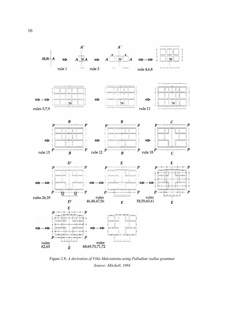
16
Figure 2.8: A derivation of Villa Malcontenta using Palladian viallas grammar
Source: Mitchell, 1994
17
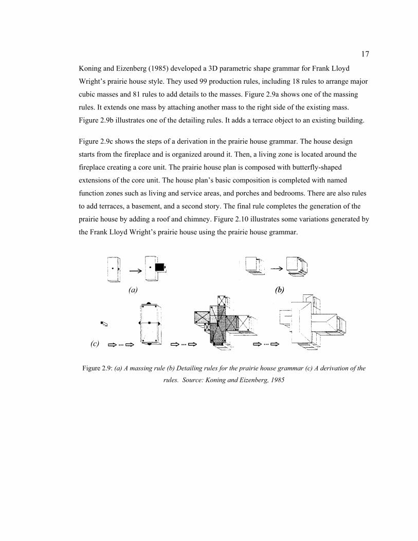
Koning and Eizenberg (1985) developed a 3D parametric shape grammar for Frank Lloyd
Wright’s prairie house style. They used 99 production rules, including 18 rules to arrange major
cubic masses and 81 rules to add details to the masses. Figure 2.9a shows one of the massing
rules. It extends one mass by attaching another mass to the right side of the existing mass.
Figure 2.9b illustrates one of the detailing rules. It adds a terrace object to an existing building.
Figure 2.9c shows the steps of a derivation in the prairie house grammar. The house design
starts from the fireplace and is organized around it. Then, a living zone is located around the
fireplace creating a core unit. The prairie house plan is composed with butterfly-shaped
extensions of the core unit. The house plan’s basic composition is completed with named
function zones such as living and service areas, and porches and bedrooms. There are also rules
to add terraces, a basement, and a second story. The final rule completes the generation of the
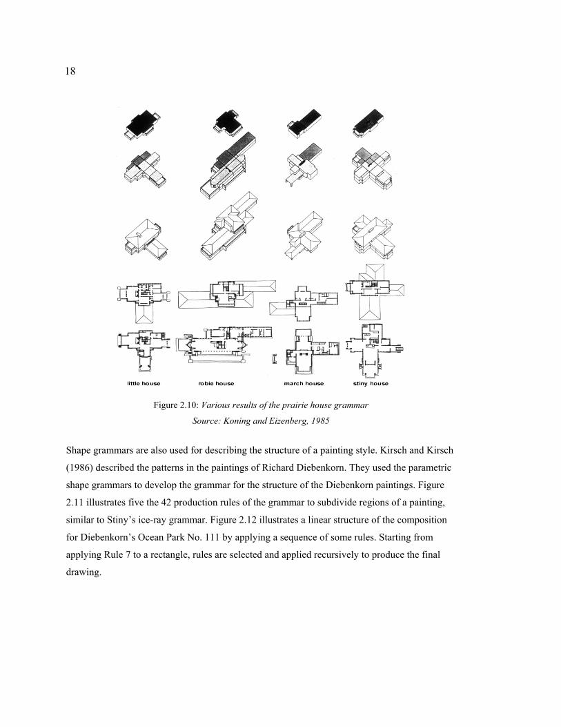
prairie house by adding a roof and chimney. Figure 2.10 illustrates some variations generated by
the Frank Lloyd Wright’s prairie house using the prairie house grammar.
(a) (b) (b)
(c)
Figure 2.9: (a) A massing rule (b) Detailing rules for the prairie house grammar (c) A derivation of the
rules. Source: Koning and Eizenberg, 1985
18
Figure 2.10: Various results of the prairie house grammar
Source: Koning and Eizenberg, 1985
Shape grammars are also used for describing the structure of a painting style. Kirsch and Kirsch
(1986) described the patterns in the paintings of Richard Diebenkorn. They used the parametric
shape grammars to develop the grammar for the structure of the Diebenkorn paintings. Figure
2.11 illustrates five the 42 production rules of the grammar to subdivide regions of a painting,
similar to Stiny’s ice-ray grammar. Figure 2.12 illustrates a linear structure of the composition
for Diebenkorn’s Ocean Park No. 111 by applying a sequence of some rules. Starting from
applying Rule 7 to a rectangle, rules are selected and applied recursively to produce the final
drawing.

19
Figure 2.11: A part of the rules for a Diebenkorn Ocean Park Grammar
Source: Kirsch and Kirsch, 1986
Figure 2.12: Steps in the generation of Diebenkorn’s Ocean Park No. 111 from the grammar
Source: Kirsch and Kirsch, 1986
Flemming (1990) presented grammars for various architectural languages: wall architecture,
mass architecture, panel architecture, layered architecture, structure/infill architecture, and skin
architecture. The goal of these grammars was to help students learn architectural composition
using rules of the languages expressed computationally. He used shape grammars to define rules
that illustrate how architectural elements can be placed in the space. For example, Figure 2.13a
shows a grammar for wall architecture, one of the languages. The rules of this grammar specify
how one wall can attach to another. Figure 2.13b illustrates some wall configurations generated
by applying the rules repeatedly. Other architectural languages can be described in a similar

20
way. Students can use a computer to explore and make compositions within these architectural
languages with a computer. They can use the grammars to learn about the languages.
Figure 2.13: (a) Generation rules for wall architecture (b) Configurations generated by these rules.
Source: Flemming, 1990

21
2.1.3. Analysis and Generation of Style with Other Algorithmic Approaches
Kirsch and Kirsch (1998) analyzed Miro’s Constellation series paintings to study Miro’s style.
They scanned Miro’s drawings and manually traced the outlines of the shapes. Through these
processes, they define classes of shapes for Miro’s paintings. Then they made several programs,
each of which controls one of the shapes. Each shape can be modified by the system in various
ways such as horizontal and vertical stretching, sizing, and rotating. Figure 2.14a illustrates the
interface of the program, “Make Anthropomorph Shape”. This program, developed in
Macintosh Common Lisp, allows a designer to change the anthropomorph shape by
manipulating a set of slide bars. Figure 2.14b illustrates the variations of the anthropomorphic
shape generated in this system. Figure 2.15a describes a set of prototype shapes captured from
the original Miro’s painting. Finally, these shapes are translated, rotated, and stretched and
synthesized into the Miro like composition [2.15b].
(a) (b)
Figure 2.14: (a) Snapshot of a program, “Make Anthropomorph Shape” (b) Various anthropomorphic
shapes generated by the program. Source: Kirsch and Kirsch, 1998

22
(a) (b)
Figure 2.15: (a) Prepared shapes from analyzing Miro’s painting (b) A final Miro composition generated
by using the prepared shapes. Source: Kirsch and Kirsch, 1998
Hersey and Freedman (1992) developed the PlanMaker computer program, to generate possible
Palladian building plans. This system, developed independently from Stiny and Mitchell’s
approach, uses a simple split system that divides a rectangle horizontally or vertically and then
resplit the previously split rectangles. This split system consists of three characteristics: a split
direction (horizontal, vertical, or both), room number and split ratio. The room number decides
how many rooms will be split. The split ratio defines the proportions of the resulting room.
These simple split system generates horizontally symmetrical and modular villa plans like
Palladio’s.
Figure 2.16 shows the sequential five stages of the split system to generate the plan of Villa
Valmarana at Lisiera in the PlanMaker system. The first stage illustrates how the initial
rectangle is split horizontally into three new rooms. Then each new room is divided vertically,
again following a specific ratio. Following the splitting rule, the PlanMaker generates the
original Palladian plan. Moreover, it allows users to generate new drawing plans in the
Palladian style. Figure 2.17 shows a variation of possible Palladian plans.

23
g
Figure 2.16: Generation of a P
Source: Hersey
Figure. 2.17: Possible Palladian vi
Source: Hersey
2.2. GENERATIVE APPLICATIONS
2.2.1. Shape Grammar Interpreters
Tapia (1999) developed GEdit, a two-dimens
interface for users to make or control the rule
shapes and defines the rules in the graphic wi
another window.
Stage 1
alladian villa in PlanMak
and Freedman, 1992
lla plans generated in Plan
and Freedman, 1992
ional shape grammar int
s for spatial layout [Fig.
ndow. The result of appl
Stage 2
Stage 5 Stage 4 Stage 3Original Drawin
er system
Maker system
erpreter that provides an
2.18]. A designer arranges
ying the rules is shown in

24
Figure 2.18: Screenshot of GEdit Interface
Source: Tapia, 1999
Mcgill (2000) developed Shaper 2D as an interpreter for standard shape grammar with a graphic
interface. It allows designing two rules at the same time with result displayed in the same
window [Fig. 2.19]. It helps the designer to test many alternative rules in a short time. Shaper2D
was used in a studio as a tool for learning shape grammars and generating shapes to inform a
design process. Figure 2.20 illustrates the process of applying the generated result to the design
process. The designer first generated 2D shape configurations in Shaper 2D [Fig. 2.20a] and
then placed it on a site drawing in CAD system [Fig. 2.20b]. Finally, the designer further
developed the 2D shape into an architectural building plan [Fig. 20c].
Figure 2.19: Screenshot of Shaper 2D Interface
Source: Mcgill, 2000
25
(a) (b) (c)
Figure 2.20: Illustrations for using the result of Shaper2D in the design process (a) The generated result
in Shaper 2D (b) Site planning with the result (c) Plan designing with the result
Source: Mcgill, 2000
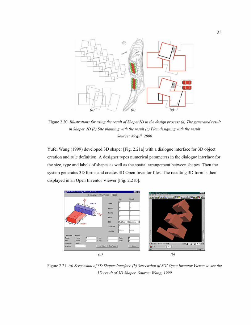
Yufei Wang (1999) developed 3D shaper [Fig. 2.21a] with a dialogue interface for 3D object
creation and rule definition. A designer types numerical parameters in the dialogue interface for
the size, type and labels of shapes as well as the spatial arrangement between shapes. Then the
system generates 3D forms and creates 3D Open Inventor files. The resulting 3D form is then
displayed in an Open Inventor Viewer [Fig. 2.21b].
(a) (b)
Figure 2.21: (a) Screenshot of 3D Shaper Interface (b) Screenshot of SGI Open Inventor Viewer to see the
3D result of 3D Shaper. Source: Wang, 1999

26
2.2.2. Algorithmic Shape or Form Generation
Different from shape grammar applications, another approach for generating form generation is
algorithmic shape generation. Algorithmic shape generation systems allow users to program
simple algorithms to generate shapes. Using user-programmed procedures, the systems generate
2D drawings or 3D geometric forms. These applications enable designers to use a computer to
algorithmically generate shapes and forms without leaving a difficult programming language.
The Logo programming environment supports a designer to create and manipulate shapes by
typing a series of instructions or writing procedures for the computer to execute. Papert and
Feurzeig (1967) created the first version of Logo with a team from Bolt, Beranek and Newman.
Logo is easy to use and learn. It has been developed over the past 36 years. Logo has been used
to design programs for various purposes such as constructive learning, mathematics, language,
music, robotics, telecommunications, and science.
Designers can explore formal design ideas by making an algorithm for shape generation in Logo.
The Logo programming environment uses a Turtle [Fig. 2.22a] that can be directed by
commands typed at the computer. For example, the command [forward 50] causes the turtle to
move forward in a straight line 50 "turtle steps". The command [right 90] rotates the turtle 90
degrees clockwise without moving any step. Then [forward 50] causes it to go forward 50 steps
in the new direction. The turtle generates a square shape following the sequential commands
[Fig. 2.22b]. This square can also be used as a procedure in a later instruction. Repeating the
commands, while rotating 10 degree each turn the turtle generates a flower-like shape [Fig.
2.22c].
This sequence of commands shows one way of generating shape configurations with simple
operations. This simple process of Logo Programming is used in various systems for design like
Design By Number (Maeda, 1999) and FormWriter (Gross, 2000). These two projects provide a
symbolic language with which users can write (and debug) formal descriptions of geometric
objects, which are then rendered visually by the program.

27
forward 50 right 90 forward 50 right 90
forward 50 right 90 forward 50 right 90
(a) the initial turtle (b) to generate “square” shape with turtle commands
repeat in [square right 10] (c) to generate “flower” shape by
manipulating the square
Figure 2.22. The turtle commands to generate shape configuration in Logo Programming Environment.
Source: http://el.media.mit.edu/logo-foundation/
Maeda (1999) developed a two-dimensional programming system called Design by Number
[Fig. 2.23]. He implemented this system as a tool for teaching computational design to
designers and artists. Design by Number introduced the basic ideas of computer programming
within the context of drawing. For example, visual elements such as dot, line, and field are
combined with the computational ideas of variables and conditional statements to generate
images. Figure 2.23 shows the interface of the system. The interface allows a designer to write
simple code and use the code to produce visualization (2D images). Figure 2.24 shows the
various results produced using different user-programmed algorithms.
Figure 2.23: Snapshot of Design by Number Interface
Source: http://dbn.media.mit.edu/

28
Figure 2.24: Various Results of Design by Number
Source: http://dbn.media.mit.edu/
Gross (2001) developed FormWriter, a simple and powerful generative system for generating
three-dimensional geometry. With only a few lines of code, a designer generates interesting
three-dimensional graphics immediately. This programming language enables architects to
explore 3D geometry form by simple programming.
Figure 2.25: Snapshot of FormWriter Interface
Source: Gross, 2001
29
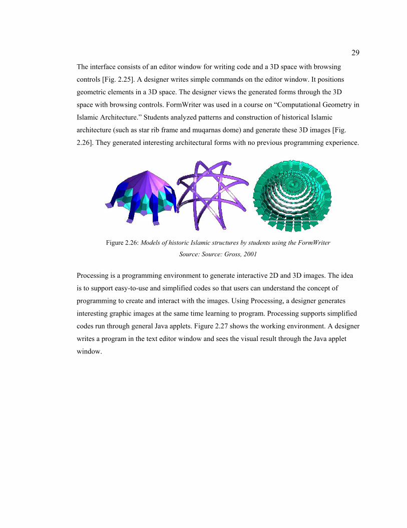
The interface consists of an editor window for writing code and a 3D space with browsing
controls [Fig. 2.25]. A designer writes simple commands on the editor window. It positions
geometric elements in a 3D space. The designer views the generated forms through the 3D
space with browsing controls. FormWriter was used in a course on “Computational Geometry in
Islamic Architecture.” Students analyzed patterns and construction of historical Islamic
architecture (such as star rib frame and muqarnas dome) and generate these 3D images [Fig.
2.26]. They generated interesting architectural forms with no previous programming experience.
Figure 2.26: Models of historic Islamic structures by students using the FormWriter
Source: Source: Gross, 2001
Processing is a programming environment to generate interactive 2D and 3D images. The idea
is to support easy-to-use and simplified codes so that users can understand the concept of
programming to create and interact with the images. Using Processing, a designer generates
interesting graphic images at the same time learning to program. Processing supports simplified
codes run through general Java applets. Figure 2.27 shows the working environment. A designer
writes a program in the text editor window and sees the visual result through the Java applet
window.

30
Figure 2.27: Snapshot of Processing Working Environment
Source: http://www.proce55ing.net/
2.3. DISCUSSION
As discussed above, a particular design style can be analyzed and described into various
computer algorithms. Drawings are used for analysis of style. A particular drawing is analyzed
by identifying the drawing elements and their relationships. A computer system can be
developed with algorithms to demonstrate a generation process for the stylistic drawing. A
designer can understand and learn a design style using the system, and develop his or her own
design style.
Generative systems enable a designer to explore formal design ideas in the early design process.
The algorithms for design style can be used to develop generative systems for design. The
generative systems should provide interfaces that allow a designer to control the generalized
algorithms. Therefore, the designer can use the algorithms in his or her own design process.
This chapter introduced several approaches for the analysis of style as well as generative
systems for 2D drawing and 3D forms. In the following chapters, this thesis describes an
analysis application for Peter Eisenman’s design style, ArchiDNA. ArchiDNA shows the
process needed to generate Eisenman-like drawings with a set of operations. Next, the thesis
proposes ArchiDNA++, a generative system. ArchiDNA++ provides an interface that allows a
designer to use the application process by controlling the design parameters.

31
Chapter Three
An Eisenman Design Machine
3. ArchiDNA
This chapter describes ArchiDNA, a system for generating designs in the style of Peter
Eisenman. It describes Eisenman’s style as a set of operations and demonstrates the use of the
operations to generate shape configurations in Eisenman’s style.
ArchiDNA is based on two assumptions. First, a certain design style can be programmed into a
set of operations. Second, those operations can be used to generate design works in the same
style following a certain process. The prototype ArchiDNA program described in this chapter
was built to explore how a designer can generate shape configurations to illustrate a certain
design style by following a certain process and a set of operations.
This chapter first explains a certain design style with its 2D and 3D drawings. It describes 2D
shape configurations with 2D operations and the process of converting 2D configurations into
3D form. Finally it summarizes the generation process of ArchiDNA and discusses the
limitations of the system.
3.1. EISENMAN’S BIOCENTRUM BUILDING DESIGN
Peter Eisenman is a famous contemporary American architect. He usually creates drawings to
find formal design idea from his design concept (Eisenman, 1996). The starting point of our
ArchiDNA project was an analysis of Peter Eisenman’s drawings of the design of his
Biocentrum building plan in Frankfurt, Germany [Fig. 3.1a]. In this project, Eisenman used
drawing both to search for a form and idea, and also to explain how the form and idea can be
manipulated as a motif and style (Eisenman, 1996).

32
Eisenman generated the building form by manipulating shapes that represent the four elements
of DNA structure: Adenine (A), Guanine (G), Cyanine (C), and Thymine (T) [Fig. 3.1b]. Four
distinct shapes are commonly used to represent these amino acids: arch (A), ribbon (G),
pentagon (C) and wedge (T) [Fig. 3.1c], and Eisenman used these as the building blocks for his
Biocentrum design. We chose this work because Eisenman’s drawings express geometry that is
describable and measurable. We hypothesized that his formal idea could be represented as
computer algorithms that manipulate the design components.
(a) (b) (c)
Figure 3.1: (a) Biocentrum (Eisenman, 1996) (b) Diagram of DNA showing Amino Acids (c) Four distinct
shapes in Amino Acids. Source: Eisenman, 1999
Eisenman’s 2D and 3D drawings illustrate how the form of the building came from abstract
representations of DNA structure. In the 2D drawing [Fig. 3.2a], four shapes represent the four
elements of DNA structure (A-T-C-G), were translated and transformed to compose the final
drawing. In the 3D drawing, the 2D drawings were extruded into a 3D form [Fig. 3.2b].

33
(a) (b)
Figure 3.2: Drawings for Biocentrum (Eisenman, 1996)
(a) Plan (b) Axonometric View. Source: Eisenman, 1999
3.2. 2-D OPERATIONS
Analyzing Eisenman’s 2D drawing, we find the primitive operations of the 2D shape
configurations. A set of shapes are translated, rotated, and scaled and attach to other shapes.
This section first explains how the primitive operations attach one shape to another. Then it
describes the applying process that generates Eisenman-like drawing.
3.2.1. Primitive Operations in ArchiDNA
We attach a shape to another shape following three main operations: translation, rotation, scale.
The three operations are basic ways to change a shape: translation (moving it somewhere else),
rotation (turning it around) and scaling (making it bigger or smaller). They are best understood
graphically. Figure 3.3 illustrates the three operations (move, rotate, and scale) of rectangle
shape to a certain point in 2D Cartesian coordinate space. The three values for the operations
are: (10, 10) for location, 45 degree for angle, and 50% for scale. The rectangle is first
translated from (0, 0) to (10, 10) degree clockwise [Fig. 3.3a], rotated from 0 to 45 [Fig. 3.3b]
and finally scaled to 200% size [Fig. 3.3c]. Scaling a shape simply means making it bigger or
smaller. A “scale factor” specifies how much bigger or smaller. For example to double the size

34
of a shape we use a scale factor of 200%, to reduce to half size of an object we use a scale factor
of 50%.
location (10, 10) angle (45 ) scale (200%)
(a) Translation (b) Rotation (c) Scaling Figure 3.3: Primitive Shape Operations
Figure 3.4 illustrates the process of applying a rectangle (square) to a line. Given a certain line
which has a location, direction, and a size in the 2D space, we can use then the information to
move the square to the location, rotate the square to be parallel to the line, and finally scale the
square to fit the size of line [Fig. 3.4].
Figure 3.4: A square is attached to a line considering its location, angle, and size
In the same way, if we use a square instead of a line, we can apply four squares following the
operations (translation, rotation, and scaling). Figure 3.5 illustrates how the rectangles are
attached to the four edges of the first square.
35
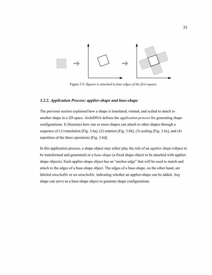
Figure 3.5: Square is attached to four edges of the first square.
3.2.2. Application Process: applier-shape and base-shape
The previous section explained how a shape is translated, rotated, and scaled to attach to
another shape in a 2D space. ArchiDNA defines the application process for generating shape
configurations. It illustrates how one or more shapes can attach to other shapes through a
sequence of (1) translation [Fig. 3.6a], (2) rotation [Fig. 3.6b], (3) scaling [Fig. 3.6c], and (4)
repetition of the three operations [Fig. 3.6d].
In this application process, a shape object may either play the role of an applier-shape (object to
be transformed and generated) or a base-shape (a fixed shape object to be attached with applier-
shape objects). Each applier-shape object has an “anchor-edge” that will be used to match and
attach to the edges of a base-shape object. The edges of a base-shape, on the other hand, are
labeled attachable or un-attachable, indicating whether an applier-shape can be added. Any
shape can serve as a base-shape object to generate shape configurations.

36
(a) Translation (b) Rotation (c) Scaling
Point 3
A: applier-shapeB: base-shape
(d) Repetition
A
A A
A
A
B
Figure 3.6: Four Shape Operations with applier-shape to base-shape
If there is more than one applier-shape object, they attach to a single base-shape object in
sequence. For example, Figure 3.7 illustrates the four different shapes (A1-A2-A3-A4) applied
to the base-shape B. It starts with the shape A1 and attaches other shapes in counter-clockwise
sequence.
A1, A2, A3, and A4: applier-shapesB: base-shape
++ + +IA1 A2 IA3 A4
I
I
A4
A1A2
A3 A1B
Figure 3.7: Four shapes (A1-A2-A3-A4) applied sequentially to the edges of the base-shape B. Note that
shape A1 occurs twice because the application process repeats at the beginning once the sequence is
exhausted.

37
3.3. 2-D GENERATION
Figure 3.8: Initial shape in ArchiDNA Interface
Following the application process, ArchiDNA generates 2D shape configurations similar to
Eisenman’s plans for the Biocentrum building. To demonstrate the process in ArchiDNA, we
start with eight shapes (2 copies of each of the four DNA shape elements) [Fig. 3.8].
Figure 3.9: (a) Applicat
(a)
ion the applier-shape G (ribbon) to the base-shape C
the applier-shape G to the base-shape A (arch)
(b)
(pentagon) (b) Application

38
The first step is to apply the shape G (ribbon) as applier-shape to the shape C (pentagon) [Fig.
3.9a]. The designer presses the “A” icon for setting applier-shape in the tool palette and selects
the G shape. Then to select the C as base-shape the designer presses “B” icon, the designer
selects the C shape (pentagon). Now that the designer has provided ArchiDNA a base-shape
object and an applier-shape object, ArchiDNA goes to work. ArchiDNA copies and attaches the
applier G shapes (ribbon) to every edge of the base C shape (pentagon) [Fig. 3.9a]. The G
shapes are attached at the short edge of the ribbon G shape because this is that shape’s anchor-
edge. Figure 3.9b demonstrates this process with a base-shape A (arch), which has eight edges
including five short line segments that approximate the curve. Eight applier ribbon (G) shapes
are generated and attached to the edges of the base-shape A [Fig. 3.9b]. This example makes
clear that ArchiDNA scales the applier shape so that its edge dimension matches that of the
base-shape where it is attached.
Figure 3.10: ArchiDNA Second Shape Generation
We repeatedly click other shapes as base-shape, so that the shape G (ribbon) is applied to other
base-shape objects. In this way, we generate interesting configurations quickly. Figure 3.10
shows the final Eisenman-like 2D drawing. The ribbon shape is moved, rotated, and scaled
based on the edges of the various base shapes selected by the user. This example shows one
applier-shape G applied to other shapes. We use four applier-shape objects to generate an
Eisenman-like drawing [Fig. 3.11].

39
We can also define applier-shapes with the four shapes (A-G-C-T) and select a base-shape
repeatedly to generate shape configurations. Figure 3.11 shows four applier-shape objects
matched and attached to several base-shape objects to generate Eisenman-like drawings quickly
[Fig. 3.11].
Figure 3.11: 2D Eisenman-like drawing generated in ArchiDNA
3.4. 3-D OPERATATIONS
Our Eisenman-like drawing can be converted to three dimensional models with automatically
assigned heights. The height extrusion for each shape is derived from a function of its area.
Eisenman’s 3D model image [Fig. 3.2b] seemed to suggest that he used a threshold controls the
shape extrusion. If the area is larger than the threshold, the height of the shape is assigned a
negative value, so that the 3D object extrudes downwards from the ground. Otherwise, the
shape will compose a building mass projecting upward. Figure 3.12 shows that the small shape
A1 (pentagon) is extruded upwards whereas the larger shape A2 (pentagon) is extruded
downwards because its area is larger than the threshold [Fig. 3.12b&3.12c]. On the other hand,
one can also assign a fixed value to the height of a shape. Shape B (ribbon) is extruded with
such given values [Fig. 3.12d].

40
A1
A2B h1
h2h1 = area of A1h2 = area of A2
area of A2 < threshold
area of A1 > threshold
height of B = user-defined height
( a ) ( b ) ( c ) ( d )
A1
A2
B
Figure 3.12: 3D form generation in ArchiDNA
(a) Calculating the area of two applied shapes A1&A2 and assigning heights (b) Comparing areas with
a threshold and deciding up and down (c) Extrusion of small shape A1 upward and extrusion of large
shape A2 downward (d) Extrusion of shape B with a user-defined height.
3.5. 3-D GENERATION
Following these 3D extrusion operation rules, ArchiDNA automatically generates 3D objects by
extruding the 2D drawings and exporting a 3D VRML file. Figure 3.13 shows a 3D Eisenman-
like model generated in ArchiDNA. The eight shapes (two pairs of A-T-G-C shapes) in the
center are extruded by a certain user-defined height. Other shapes were extruded to a height that
is a function of their area.
Figure 3.13: 3D Eisenman-like Model Generated in ArchiDNA

41
3.6. SUMMARY
We generated 2D and 3D Eisenman-like drawings by applying a set of geometric operations
(translating, rotating, and scaling) to applier-shapes and attaching them to the edges of a base-
shape. Figure 3.14 shows the four steps of ArchiDNA. Designers define one or more applier-
shapes, and then select a base-shape. ArchiDNA then generates 2D shape configuration and 3D
form. Following this simple process, a designer can generate Eisenman-like drawings in a very
short time. Even a beginner can learn and use ArchiDNA.
Define applier-shape(s)
Select base-shape
2D Shape Configuration
3D Form Generation
Figure 3.14: Four steps of process to generate Eisenman-like drawing
3.7. DISCUSSION
We developed ArchiDNA to generate Eisenman-like configurations according to a simple set of
operations. The designer defines applier-shape objects and selects base-shape objects. The
duplicates of applier-shape objects then attach to the edges of the selected base-shape objects.
ArchiDNA shows a simple and interesting process to generate Eisenman’s drawings. It is easy
to use and learn. A complicated 2D shape configurations and 3D forms in the Eisenman’s style
can be generated quickly. What if we like to generate drawings of other style? Here are the
perceived limitations of ArchiDNA:

42
• ArchiDNA operates with only four built-in shapes (A-T-G-C).
• A designer cannot control the shape operations (pre-set rotation and scaling).
• A designer cannot change the shape attributes of where and how applier-shape can attach to a base-shape (attachable-edge of base-shape object and anchor-edge of applier-shape).
The strength of ArchiDNA is to generate Eisenman-like drawing for Biocentrum Building.
What if designers want to use the system to generate other kinds of drawing? Can we generalize
the generation process in ArchiDNA to provide a method to generate 2D shape configurations?
A system like ArchiDNA can be a generation tool for other type of shape configurations. Can
we use the same kind of application process to generate drawings of other style? Therefore, the
thesis proposes an extension of ArchiDNA, called ArchiDNA++ to enable more manipulation
and control of the generation process. Next chapter describes the implementation of
ArchiDNA++ system to support control of the geometric operations and to create shapes for
both applier-shape and base-shape. It also explains how a designer can utilize the ArchiDNA++
to produce shape configurations.

43
Chapter Four
An End-User Programming Environment For Shape Configuration
4. ArchiDNA ++
ArchiDNA++ is an extension of ArchiDNA, a generative system for shape configurations. The
development of ArchiDNA++ focuses on making the application process available with a
variety of operations. Instead of just generating Eisenman-like drawing in Chapter 3, the goal of
ArchiDNA++ is to generalize the application process for generating shape configurations with
other user-defined styles. This is to facilitate more flexibility for a designer to generate shape
configurations for his or her design work.
In the previous section, We noted some limitations of ArchiDNA. It only supports using
predefined (A-G-C-T) shapes and a pre-set translation to all edges of selected base-shapes to
generate Eisenman-like drawings. To address these limitations, ArchiDNA++ provides an
interface that allows users adjust and control the operation parameters. ArchiDNA++ has the
following features to support generations of shape configurations:
1. A designer can create his or her own shapes as applier-shape and base-shape.
2. A designer can manage applier-shape list for the order of applier-shapes.
3. A designer can change shape operations and attributes for modifying shape configurations.
4. A designer can generate shape configurations by drawing a base-shape as well as selecting a base-shape.
5. A designer can control 3D conversion operations by setting height or threshold to different shapes.
This chapter is divided into four sections: Section 4.1. describes the work environment of
ArchiDNA++. Section 4.2. explains the overivew of ArchiDNA++ operations. Section 4.3.
describes shape preparation phase including shape creation and the attribute control. Section 4.4.

44
explains shape configuration process with applier-shape and base-shape. Section 4.5 discusses
the conversion from 2-D to 3-D. Finally Section 4.6 introduces an example to generatea
sunflower shape using ArchiDNA++.
4.1. ARCHIDNA++ ENVIRONMENT
The work environment is an important feature of ArchiDNA++. The generation process in
ArchiDNA was hidden from the designer; designers could not change or control the process. It
will only produce Eisenman-like drawing. However, most designers would like to use their own
shapes and control the rules to generate shape configurations to represent their own personal
thinking and style. ArchiDNA++ attempts to make the configuring process as transparent as
possible with the interface that provides a work environment to create shapes and control the
generation process.
The main purpose of developing the work environment is to allow a designer to create applier-
shape and base-shape for his or her own design. For this purpose, the system must provide an
interface to support the designer in generating shapes and to program the operation of shape
configuration.
The work environment of ArchiDNA++ has three main parts [Fig. 4.1]: at top a tool palette, at
left a window consisting of a drawing panel and a configuration panel with a view palette; at
right a control window. The control window has four palettes: a drawing palette [Fig. 4.2a], an
attribute palette [Fig. 4.2b], a list palette [Fig. 4.2c], and a 3D palette [Fig. 4.2d].
4.1.1. Tool Palette
The tool palette is at the top of the screen and consists of eight buttons. Pressing each button at
the first row displays its corresponding panel in the control window at the right. Four buttons on
the second row are used to export 3D VRML files, saving and opening an ArchiDNA++ file,
and showing version information about this system.

45
4.1.2. Drawing Window
The Drawing Window is composed of three panels divided horizontally: the configuration panel,
drawing panel and view palette. The configuration panel (upper) is for generating shape
configurations, and the drawing panel (lower) is for drawing shapes for applier-shape and base-
shape. Users can change the size of each panel by moving the resize button between the two
panels. This separated drawing area helps users to draw, organize, and set applier- and base-
shapes. The view palette at the bottom allows users to zoom in or out, turn grid and grid
snapping on and off for the configuration panel and drawing panel.
4.1.3. Four Control Palettes
Once the designer creates shapes in the drawing panel using the drawing palette, the designer
controls shape attributes with the attribute palette and defines applier-shape(s) using the list
palette. ArchiDNA++ has four control palettes displayed in the control window: drawing palette,
attribute palette, list palette, and 3D palette [Fig. 4.2]. The designer switches from one to
another by simply pressing the four corresponding buttons in the tool palette.
(a) Configuration Panel
(b) Drawing Panel
Figure 4.1: Snapshot of ArchiDNA++ Interface

46
(a) Drawing Palette (b) Attribute Palette (C) List Palette (d) 3D Palette
Figure 4.2: Four Control Palettes
4.2. ARCHIDNA++ IN USE
A designer uses ArchiDNA++ in three phases: Shape Preparation, Shape Configuration, and 3D
Conversion. Figure 4.3 illustrates the three phases with five new steps (gray boxes) in addition
to the steps described in the previous section for ArchiDNA [Fig. 3.14]. It supports an easy and
powerful process not only to generate Eisenman-like drawings but also to describe and generate
drawings in other styles. We next describe this process in detail.

47
Define applier-shape(s)
Select base-shape
2D Shape Configuration
Set 3D Mode
Shape Creation Shape Attribute Control
Draw base-shape
Set Threshold
Shape Preparation Phase
Shape Configuration Phase
3-D Conversion Phase
Figure 4.3: Overview of ArchiDNA++ Operation
4.3. SHAPE PREPARATION PHASE
The Shape Preparation Phase prepares shapes to be used as applier-shape and base-shapes. If a
designer already has previously prepared shapes, this phase can be skipped. This phase has two
sub-processes: Shape Creation and Shape Attribute Control. Once a shape is created, it can be
used for application to without going through the Shape Attribute Control process. The Shape
Attribute Control is optional. It provides a greater flexibility for further manipulation of the
shapes.
4.3.1. Shape Creation
The designer can create various shapes in the drawing panel [Fig. 4.4 & bottom of Fig. 4.1].
ArchiDNA++ provides tools for drawing (line, poly-line, rectangle, sketch, and text) and editing
(select, move, rotate, and delete) in the drawing palette [Fig. 4.2a] like other CAD software. For
example, to draw a rectangle shape, the designer first selects a button for “draw rectangle” in

48
the drawing palette, and clicks in the drawing panel. A rectangle is rubber banded as the
designer moves the mouse. When the designer clicks again, a rectangle is created and displayed
in the drawing panel. To create lines and polygons, a similar click-click process is used.
The sketch tool lets the designer draw continuous sketch lines. The designer first selects the
button for “draw sketch”, click to begin, and then drag the mouse freely to draw some shape.
Then the designer releases the mouse to stop drawing. Designers can also use a pen tablet to
draw. The sketch line drawn consists of little line segments with control points generated by the
program automatically. Changing the drawing speed would vary the distance between the
control points.
Figure 4.4 shows the default shape attributes of a rectangle shape: name, area of the shape,
direction, angle, and scale-factor of each edge. A user can control the Application process by
changing these attributes. The next section explains controlling the attributes in detail.
Figure 4.4: Created Shapes – left: attributes of a rectangle shape, and a small red-rectangle label
(¬) in the center of an edge marks an anchor-edge (for lines and poly-lines).
4.3.2. Shape Attribute Control
In Figure 3.6, we generated a shape configuration by applying an applier-shape object (ribbon)
to a base-shape object (pentagon). In ArchiDNA++, a designer can explore and generate more
variation of shape configurations simply by changing shape attributes: anchor-edge, attachable-
edge, operation values (angle and scale), and direction. An attribute palette [Fig. 4.2b] is
provided for this manipulation process.

49
Figure 4.5 illustrates how the designer can change the anchor-edge from the top-side edge
(default) to the right-side edge in an applier-shape object. The system will then generate a
configuration by matching and attaching the right-side edge to all edges of a base-shape object.
The default operation generates a radiating pattern of ribbon shapes rooted from the pentagon
[dashed line]. Once the anchor-edge of the applier-shape moves to the right edge, the result is a
continuous head-to-tail ribbon stripes surrounding the pentagon.
anchor-edge
+
A: applier-shape B: base-shape
Figure 4.5: Changing anchor-edge of applier-shape object (ribbon) and the result of applying it to a
base-shape object (pentagon); dotted lines illustrates the default configuration that uses anchor-edge at
the top of ribbon.
The designer can also change attachable-edges to un-attachable edges. Figure 4.6 shows when
two edges of the base-shape object are made un-attachable, those two edges of the base-shape
object will not have any instance of the applier-shape object in the result.
un-attachable-edges
anchor-edge
B A
A
A
A: applier-shape B: base-shape
Figure 4.6: Change two attachable-edges of base-shape object (pentagon) to un-attachable edges and its
result with an applier-shape object (ribbon).

50
The designer can also control shape operations (rotation and scaling) by setting operation values
(angle and scale-factor) to an edge of a base-shape object. By default, the applier-shape object
matches and attaches to an edge of a base-shape object as in ArchiDNA [Fig. 3.6]. Figure 4.7
shows a different result of fixing the base-shape’s three edges with a certain angle (90°) and a
scale factor (50%) in ArchiDNA++. The three applier-shape objects were translated to each
edge of the base-shape object and rotated and scaled with user-defined values (not matching the
base-shape object).
user-fixed edges- angle: 90- scale-factor: 50%
anchor-edge
A: applier-shape B: base-shape
o
A
BA
A
A
A
Figure 4.7: Fix three edges with angle (90°) and scale-factor (50%) and its result shows three applier-
shape objects are not matched to the base-shape object.
In addition to these three attributes, a designer can reverse the direction of a base-shape object
from counter-clockwise (default) to clockwise. Figure 4.8a shows how four applier-shape
objects (A1-A2-A3-A4) attach to the default base-shape object in sequence following the
direction, counter-clockwise [also see Fig. 3.6]. If the designer changes the direction to
clockwise, the four applier-shape objects attach in sequence, clockwise, generating a different
shape configuration [Fig. 4.8b].

51
IA1
B
I
I
A4
A1A2
A3 A1B
A1
IA3
A2A4
(a) counter-clockwise (b) clockwise
starting applier-shape object
Figure 4.8: (a) Counter-clockwise base-shape object (b) Clockwise base-shape object with four applier-
shape objects (A1-A2-A3-A4)
4.4. SHAPE CONFIGURATION PHASE
The Shape Configuration Phase generates shape configurations with applier-shapes and base-
shapes. In the configuration panel, designers proceed to the “application-process” using the
shapes drawn in the drawing panel.
4.4.1. Define applier-shape(s)
The list palette consists of two sub-lists: an applier-shape list (upper) and an all-shape list
(lower) [Fig. 4.2c]. A designer can see the sequential list of applier-shapes and all shapes. The
designer defines applier-shape list using drag and drop from the all-shape list to the applier-
shape list.
4.4.2. Select base-shape or Draw base-shape
Designers can generate new shapes by choosing or drawing a base-shape object in the
configuration panel. When drawing a base-shape, designers use the drawing palette in the same
way, as one would do in creating a shape in the drawing panel.

52
Figure 4.9 shows various shape configurations generated in ArchiDNA++. Figure 4.9a
illustrates result of drawing a curved line as a base-shape. As small-segmented lines
approximate the curve line, the instances of the applier-shape (ribbon) are attached to the curve
following the segmented lines. Figure 4.9b shows an interesting result when a ribbon-like shape
is used as applier-shape and base-shape at the same time. Figure 4.9c shows the resulting
pattern when a single human figure as applier-shape is applied to a rectangle base-shape. It
generates a pattern reminiscent of the work of M.C. Escher.
4.5. 3-D
ArchiDN
object ac
of a clos
shape by
(a)
Figure 4.9: Various Shape Configurations in ArchiDNA++
CONVERSION
A++ converts 2D shape configurations into 3D forms by assigning heights to e
cording to its shape. The system assigns the height automatically using the area
ed-shape or the boundary length of an open-shape. A designer can also fix a hei
defining a certain value through the 3D palette in the control window [Fig. 4.2
(c)
(b)
ach
value
ght of a
d].

53
4.5.1. Threshold Setting
As explained previously [Fig. 3.12], 3D conversion in ArchiDNA operates on a certain
threshold to decide either the shape is extruded upward or downward. In ArchiDNA++, a
designer can specify a threshold value by selecting a shape of which area (closed shape) or
length (open-shape) to be used as a threshold.
4.5.2. 3D Mode Setting
Once a threshold is set, the designer can choose a mode (block or wall) to generate a 3D-object
in either block-type [Fig. 4.10a] or wall-type [Fig. 4.10b]. Block mode creates a mass model
extruding the 2D shape configurations as we generated 3D Eisenman-like drawing [Fig. 3.2b].
Wall mode converts a 2D line to a 3D wall object with a preset thickness that a designer can
define in the 3D palette [Fig. 4.2d]. Figure 4.10 shows the difference between the block mode
and the wall mode. The designer can display the converted 3D VRML model with VRML
viewer (e.g. Cortorna, Cosmo, etc) on a web-browser [Fig. 4.11a]. He or she can also export the
VRML file into other 2D or 3D formats for further manipulation such as rendering or animation
[Fig. 4.11b].
) )
(a) 3D
(a
Figure 4.10: 3D Mode: block-mode and wall-mode
model generated in block-mode (b) 3D model generated
(b
in wall-mode.

54
)
Figure 4.1
4.6. EXAMP
This section s
4.12 shows tw
generate shap
demonstrate h
Figure 4.12: (
(a)
1: (a) ArchiDNA++ 3D Model in VRML Viewer, Cortona (
imported into formZ.
LE: GENERATION OF A SUNFLOWER SH
hows how a designer uses ArchiDNA++ to generate a
o sketch drawings of sunflower shapes, which we wi
e configurations in ArchiDNA++. The scenario presen
ow to use the application process in ArchiDNA++.
(a)
a) First sketch drawing for generating a sunf1ower shape
elaborating the first sunflower shape
(b
b) ArchiDNA++ 3D Model
APE
sunflower shape. Figure
ll use later in this section to
ted here helps to clarify and
(b)
(b) Second sketch drawing for

55
The scenario is divided into two phases: shape preparation and shape configuration. The
preparation creates three shapes (triangle, hexagon, and ribbon) [Fig. 4.13] and controls those
shapes in terms of their use as applier-shape and base-shape. The configuration phase uses those
prepared shapes to generate shape configuration. There are two steps in the phase. The first step
generates sunflower-like configurations by attaching the ribbon applier-shape to the edges of the
hexagon base-shape [Fig. 4.15a] and the second step elaborates the first shape configuration by
applying the triangle applier-shape to all ribbon shapes generated in the previous step [Fig.
4.15b].
4.6.1. Shape Preparation
1) Create three shapes (hexagon, triangle, and ribbon) on the drawing panel.
The designer presses the Shape Drawing Control button, and the drawing palette appears in the
right control area, which has drawing tools such as line, rectangle, poly-line, sketch, and etc. By
choosing the “draw poly-line” button, the designer can create three shapes (hexagon, triangle,
and ribbon-like shape) in the drawing panel.
First, the designer clicks on a point, and then clicks on another line. After each click, a new line
is rubber banded that is anchored on the previous point. The designer double-clicks on the point
he wants to finish. A polygon shape is created and displayed. The double click of the mouse
signals completion of the drawing process and creates a 2D shape. Positioning the mouse on the
first point and double clicking closes a shape. Following these steps, the designer creates a
hexagon, triangle, and ribbon shape on the drawing panel [Fig. 4.13].
(a) (b) (c)
Figure 4.13: Create three shapes (ribbon, triangle, and hexagon)

56
2) Change the anchor-edge of the triangle
To attach the longest edge of the triangle to a ribbon, the designer needs to change the anchor-
edge. When creating a triangle, the default anchor-edge was right diagonal edge [Fig. 4.13]. The
designer can change the anchor-edge to the bottom edge by using the “Set anchor-edge” button
in the attribute palette. After pressing the button, the designer clicks the bottom edge and then
the small red-rectangle mark will be moved to the bottom edge [Fig. 4.14b].
3) Change the attachable edge of the ribbon-like shape
In the next step, the designer will choose a triangle as the applier-shape, and apply it to a base-
shape (ribbon). The ribbon has five attachable-edges. We would like to attach the triangle only
to the two side edges (right and left) of the ribbon shape [Fig. 4.14a]. Therefore, only two side
edges should be defined as “attachable” and other edges should be as “un-attachable”. To
change an edge to un-attachable, a designer can press the button for “set attachable” in the
attribute palette, and then selects an attachable edge. The set-attachable button toggles in
attachable mode of an edge. Figure 4.14a shows that the two attachable-edges are active sites
where other shapes may be attached.
un-attachable-edges
attachable-edges
anchor-edge
(a) (b) (c)
Figure 4.14: Change shape attributes (attachable-edge and anchor-edge)
4.6.2. Shape Configuration
1) Place the hexagon as an initial base-shape to Shape Configuration Panel
The shape configuration step starts from locating the hexagon shape to the configuration panel.
We will then attach the ribbon shape to the hexagon. First the hexagon should be moved to the
57
configuration panel as a base-shape object. Once the designer creates the three shapes (ribbon,
hexagon, and triangle), they are automatically added to the all-shape list with a default name
(Shape 1, Shape 2, and Shape 3). When selecting the “Shape 2” in the shape list, designers can
see the hexagon shape is highlighted with a red color. A designer moves the hexagon by
dragging it to the configuration panel and clicks on the configuration panel.
2) Set the ribbon shape to applier-shape list
The designer also then sets an applier-shape object. We will use the ribbon shape as the applier-
shape object. Similar to the previous example, the designer selects the “Shape 1” that represents
the ribbon in the all-shape list, and then drags the item to the applier-shape list, adding the
ribbon to the applier-shape list.
3) Generate Sunflower-like shape in the configuration panel
Now a designer can generate the first shape configuration with the applier-shape object (ribbon)
and the base-shape object (hexagon). First the designer presses the “select base” button in the
drawing palette. The designer selects a hexagon base-shape in the configuration panel. Figure
4.15a shows the resulting final shape in which ribbon shapes are attached to all edges of the
hexagon base-shape object.
4) Set the triangle to applier-shape list
This time we use the triangle as an applier-shape and attach to the already generated ribbon
shapes. First we change the applier-shape list. The designer selects the Shape 1 that represents
the ribbon we used in the previous configuration, and then moves it to the all shape list. This
deletes it from the applier-shape list. Then, in a similar way, the designer moves the triangle
from the shape list to the applier-shape list.

58
5) Select the already-generated ribbons as a base-shape object
The final step is to generate the second configurations that elaborate the first configuration with
a triangle on each side of the ribbon. When a designer select a ribbon, the triangle applier-shape
is attached to the two side edges of the ribbon. The triangles are not attached to the two diagonal
edges at top of the ribbon because they were labeled un-attachable. In this way, the designer
selects all ribbons as a base-shape object and makes the elaborated sunflower [Fig. 4.15b].
)
Figure 4.15: (a) First shape con
Second shape configuration f
(a)
figuration for sunflower-like shape attac
or sunflower-like shape attaching a trian
objects
(b
hing ribbons to a pentagon (b)
gle to the ribbon base-shape

59
Chapter Five
Implementation of ArchiDNA++
5. Implementation
This chapter explains how ArchiDNA++ is implemented. The first ArchiDNA system is a Java
Applet. It is implemented using JDK (Java Development Kit) 1.0. The system runs on any web-
browser that supports JDK 1.0. ArchiDNA++ software used some Java classes of JDK 1.4 for
implementing GUI (Graphic User Interface). To use ArchiDNA++, one needs to install JRE
(Java Runtime Environment) 1.4 in their local machine.
The implementation of ArchiDNA++ is divided into 3 parts:
• Shape Data Structure: to represent a shape as applier-shape and base-shape
• Shape Configuration: to generate shape configurations
• Exporting VRML models: to convert 2D configurations into 3D forms
5.1. SYSTEM ARCHITECTURE
ArchiDNA++ consists of three main parts: data structure, configuration system and 3D
converter. Figure 5.1 illustrates the ArchiDNA++ system architecture.
3D VRML model
Data Structure
ConfigurationSystem
3D Converter
Drawing Panel
Configuration Panel
ArchiDNA++
Shape Control
Figure 5.1: ArchiDNA++ System Architecture.

60
Configuration system generates shape configurations using the shapes created in the drawing
panel. It receives shape information from the data structure. The generated shapes in the
configuration system are stored again in the data structure. Data Structure hierarchically
manages the sub-shapes (points and lines) and represents the shapes on the computer screen.
When designers draw shapes in the drawing panel, this drawing information is sent to this data
structure. 3D converter translates the 2D configurations into a 3D VRML format. It is connected
to the data structure to retrieve the 2D shape information.
5.2. SHAPE DATA STRUCTURE
ArchiDNA++ is a 2D vector-based system. A shape in the system consists of sub-shapes (point
and edge). The application process uses the sub-shapes when attaching an applier-shape object
to a base-shape object. ArchiDNA++ has a simple data structure to represent various 2D shapes.
Figure 5.2 shows the process to construct a ribbon-like shape with sub-shapes (point and edge).
First, the system creates five points by specifying five 2D coordinates [Fig. 5.2a]. Then, the five
points are connected with five edges [Fig. 5.2b]. One of the edges is marked with a star (*) as
anchor-edge. All edges are marked with a plus (+) for attachable-edge or a negative (-) for un-
attachable-edge, and operation values (angle and scale).
point 1(x1, y1)
point 2(x2, y2)
point 5(x5, y5)
point 3(x3, y3)
point 4(x4, y4)
edge 1 (+)
edge 2 (+)anglescale
edge 5 (-)anglescale
edge 3 (+)anglescale
edge 4 (-)anglescale
*
(a) (b) (c)
anglescale
Figure 5.2: Representation of a ribbon-like shape with points and edges
(a) five points with 2D coordinates (b) five edges with anchor-edge mark [*], attachable-edge mark [+],
un-attachable-edge mark [-], and operation values [angle and scale] (c) the final display on the screen.

61
Figure 5.3 illustrates the hierarchical and object-oriented data structure for a ribbon-like shape.
A shape object references five edge objects and has an anchor-edge. Each edge object
references two point objects as a start-point and an end-point, and has an attachability (+ or -)
and an angle and a scale for shape operation. A point object has a X-coordinate and a Y-
coordinate.
point 1
x = x1y = y1
point 2
x = x2y = y2
point 4
x = x4y = y4
point 3
x = x3y = y3
point 5
x = x5y = y5
edge 1
start: point 1end: point 2
attachability: +angle: 0scale: 0
edge 2
start: point 2end: point 3
attachability: +angle: 0scale: 0
edge 3
start: point 3end: point 4
attachability: +angle: 0scale: 0
edge 4
start: point 4end: point 5
attachability: -angle: 0scale: 0
edge 5
start: point 5end: point 1
attachability: -angle: 0scale: 0
Ribbon Shape
anchor-edge:edge 1
*
Figure 5.3: Data Structure for a ribbon-like shape in ArchiDNA.
5.3. SHAPE CONFIGURATION
As explained before, ArchiDNA++ attaches one or several applier-shapes to a base-shape in a
sequence to generate a shape configuration. Figure 5.4 shows how the system generates shape
configurations by referencing shapes. The system has a shape list to store all created shape
objects. The applier-shape list is constructed with a shape ID. Therefore, when users select an
applier-shape, the ID of the selected shape is added to the applier-shape list. Using the IDs and
their sequence in this list, instances of shape objects are linked to the edges of the base-shape.
The Shape Operations module transforms the instances to match and attach to the edges. The
Shape Operation module sets a location for translation and calculates an angle for rotation and a
scale-factor for scaling, using the points of the base-shape.

62
applier-shape list
No. shape ID
1
2
3
4
14
2
3
shape list
ID shape obj.
1
2
3
4
object 1object 2
object 3
object 4point 1 point 2 point 3
edge 1 edge 2 edge 3
shape
base-shape
shape-configuration
Shape Operations
Instanceof
object1
Instanceof
object4
Instanceof
object2
Figure 5.4: A System Diagram for the Process of Shape Configuration
5.4. EXPORTING VRML MODELS
Like ArchiDNA, ArchiDNA++ converts 2D shape configurations to 3D objects in VRML
format. VRML is widely used to visualize 3D models on the Internet. Most 3D modelers can
import this format. Figure 5.5 describes the simple process that converts a 2D ribbon shape to
3D face objects of VRML. First using the x and y coordinates of the ribbon shape, the system
constructs two 3D polygons. Each polygon is constructed by adding a Z-coordinate to the 2D
coordinates of the 2D ribbon shape for height. The first polygon assigns 0 to Z-coordinate and
another assigns the shape’s area (closed shape) or length (open shape). The system sets an ID
number to each 3D coordinate in sequence. Then it generates seven 3D VRML face objects by
linking the relevant IDs. In case of an open shape, only side faces are constructed without a top
and bottom face. Through these simple steps, the ArchiDNA software converts 2D shape
configurations to 3D VRML file format.
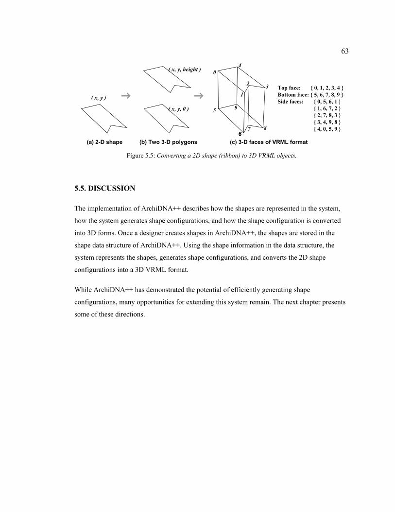
63
(a) 2-D shape (b) Two 3-D polygons (c) 3-D faces of VRML format
( x, y )
( x, y, height )
( x, y, 0 )
0
9
2 3
4
5
67 8
1Top face: { 0, 1, 2, 3, 4 }Bottom face: { 5, 6, 7, 8, 9 }Side faces: { 0, 5, 6, 1 }
{ 1, 6, 7, 2 } { 2, 7, 8, 3 } { 3, 4, 9, 8 } { 4, 0, 5, 9 }
Figure 5.5: Converting a 2D shape (ribbon) to 3D VRML objects.
5.5. DISCUSSION
The implementation of ArchiDNA++ describes how the shapes are represented in the system,
how the system generates shape configurations, and how the shape configuration is converted
into 3D forms. Once a designer creates shapes in ArchiDNA++, the shapes are stored in the
shape data structure of ArchiDNA++. Using the shape information in the data structure, the
system represents the shapes, generates shape configurations, and converts the 2D shape
configurations into a 3D VRML format.
While ArchiDNA++ has demonstrated the potential of efficiently generating shape
configurations, many opportunities for extending this system remain. The next chapter presents
some of these directions.

64
Chapter Six
Future Work and Conclusion
6. Future Work and Conclusion
6.1. FUTURE WORK
The working system of ArchiDNA++ efficiently manages generation of shape configurations
and its operations. For further exploration, there are many more features one could add to the
system. This section describes three main directions.
6.1.1. Spatial Configurations
ArchiDNA can become a tool to manipulate and transform spatial arrangements. Currently,
ArchiDNA has an object-oriented data structure to represent and operate shapes. It can be
expanded to a simple building data model that represents several building components such as
space, wall, and column. For example, we can start by replacing shape, edge and point objects
by space, wall and column objects respectively. Then we can add an opening object (window or
door) to the wall. This process could be a starting point to develop ArchiDNA as a system to
generate spatial arrangements of a floor plan.
Figure 6.1 shows the possible process to represent a ribbon space with walls, columns, windows,
and openings. Figure 6.2 illustrates a building data model for the ribbon space. Compared with
the previous data structure for a ribbon shape in ArchiDNA, this data structure also has space,
wall, column, window, and door objects. Figure 6.3 describes the possible 3D form converted
from the 2D ribbon space. The 3D wall objects are extruded with a certain thickness and have a
door or window opening.

65
window 1
door 1
point 4(x4, y4)
wall 1
wall 2wall 5
wall 3wall 4
(c)(b)
window 2
column 5 column 3
column 4
(a)
column 2column 1
Figure 6.1: Representation of a ribbon space
column 1
x = x1y = y1
column 2
x = x2y = y2
column 4
x = x4y = y4
column 3
x = x3y = y3
column 5
x = x5y = y5
wall 1
start: wall 1end: wall 2
attachability: +angle: 0scale: 0
wall 2
start: wall 2end: wall 3
attachability: +angle: 0scale: 0
wall 3
start: wall 3end: wall 4
attachability: +angle: 0scale: 0
wall 4
start: wall 4end: wall 5
attachability: -angle: 0scale: 0
wall 5
start: wall 5end: wall 1
attachability: -angle: 0scale: 0
ribbon space
anchor-wall:wall 1
*
widow 1
type: 1
door 1
type: 1
window 2
type: 2
Figure 6.2: Data structure for a ribbon space
window 1 door 1
window 2
Figure 6.3: 3D conversion of a ribbon space

66
6.1.2. ArchiDNA as a Kind of Shape Grammar
ArchiDNA uses the application process to generate shape configurations to generate Eisenman-
like drawings. It has a set of operations (translation, rotation, scaling) that attach one or several
shapes to the edges of another shape. The application process can be implemented with
replacement rules of shape grammar. A possible scenario might use the shape grammar rules for
this process. When a designer defines one or several shapes as applier-shape, each applier-shape
can be defined as a replacement rule of shape grammar. For instance, when the system sees a
single-line, it can be replaced by an applier-shape. This can be represented as a single-line shape
positioned on the left side of the arrow and one applier-shape on the right side of the arrow [Fig.
6.4 rule 2]. The applier-shape consists of line shapes, one of which has a labeled line. The
labeled line of applier-shape indicates a matching line of applier-shape when replaced with the
line. If there is more than one applier-shape, the replacement rules can be defined for each
corresponding applier-shape. Once the rules are fixed, the application process can start
replacing the lines with applier-shapes. Following the sequence of lines, the rules are applied
recursively and a shape configuration is generated.
Figure 6.4 illustrates possible shape grammar rules for the application process of ArchiDNA.
Rule 2 shows one single line is replaced with a ribbon shape. The ribbon shape consists of the
sequential five lines, one of which is labeled with a dot. The number that indicates the sequence
is used when applying the rules sequentially. The derivation shows that the ribbon shape
sequentially replaces the line of the first ribbon shape, following the numbered order of the lines.
Derivation:
Rule 1: Rule 2:
…
1 3
45
2
Figure 6.4: Rules for a grammar of ArchiDNA application process

67
Figure 6.5 shows the modified rules for the case where is more than one applier-shape (ribbon
and pentagon). Rule 2-1 replaces one single line with ribbon shape and rule 2-2 with a pentagon
shape. In derivation, these two rules are applied in sequence. Figure 6.6 also shows that rule 2-1
is applied first and then rule 2-2 is applied to the next line, following the sequential order of
lines.
…
1 3
45
2
Rule 2-1 Rule 2-1 Rule 2-2Rule 1
Derivation:
Rule 1: Rule 2-1: Rule 2-2:
Figure 6.5: Optional Rules for a grammar of ArchiDNA application process
6.1.3. 3D Form Configuration
ArchiDNA++’s current application process uses 2D shape. A future extension of ArchiDNA
can be developed to use 3D shapes and face objects for the application process. A possible
scenario can be described like this: A designer defines one or several 3D applier-shapes then
select 3D base-shape. Then the system attaches a 3D applier-shape to the faces of the 3D base-
shape. Each face has an instance of 3D applier-shape transformed with the three operations
(translation, rotation, and scaling). The operations would function with three-dimensional
coordinates (x, y, and z) in 3D space. This 3D application process will enable exploring 3D
formal design ideas by simple applying 3D shapes to another 3D shape. Figure 6.6 shows how
one 3D box applier-shape is applied to another 3D box base-shape to generate an interesting 3D
form configuration.

68
3D applier-shape
3D base-shape
3D formconfiguration
Figure 6.6: 3D form configuration of applying 3D applier-shape to 3D base-shape
6.2. CONCLUSION
This thesis presented a generative system, ArchiDNA, to generate drawing with a particular
style of Eisenman’s drawing. It has also demonstrated the extension of ArchiDNA, called
ArchiDNA++ to allow a designer to generate more variety of drawings by manipulating the
different parameter of the shapes. Developing these two systems, the thesis discusses the two
topics: analysis of design style and the making of generative design systems. The goal of this
study is to show how a generative system can be developed from a particular drawing style and
how it may be useful for exploring shape configurations in design.
ArchiDNA demonstrates that a particular Eisenman’s drawing is generated following a simple
generation process with a set of operations, called an application process. The application
process attaches one or several shapes to another shapes following the translation, rotation,
scaling operations. In ArchiDNA, a designer starts the application process with a set of shapes
(represent four DNA components, A-G-C-T). The designers define one or several shapes as
applier-shape and select another shape as base-shape. Then the system attaches the applier-
shape objects to all the edges of the base-shape object. Repeating the base-shape selecting
process will generate complex shape configuration drawing. This simple application enables a
designer to generate Eisenman-like drawing in a few seconds. ArchiDNA also converts the
generated 2D Eisenman-like drawing into 3D forms that mimic Eisenman’s 3D model for the
Biocentrum Building [Fig. 3.1a].

69
The application process in ArchiDNA is a simple way of describing Peter Eisenman’s design
style embedded in a particular drawing. With ArchiDNA, designers can learn the generation
process and generate drawings in the same style. It is simple and easy to learn and use. Thus
even first time user or beginning designer easily can generate Eisenman-like drawing. However,
ArchiDNA can only generate drawings in Eisenman style. How then, can a designer use the
powerful generation process for their design? The second part of the thesis attempts to address
this question with the implementation of ArchiDNA++.
ArchiDNA++ is a generative system for the use of the application process. This system uses the
same process that ArchiDNA uses to generate drawings in the Eisenman’s style. However, it
generalizes the generation process and supports a designer to manage the process. ArchiDNA++
enables a designer to create new shapes and control the operations. This system provides an
interface to control the generation process. In ArchiDNA++, a designer creates his or her own
shapes and controls the shapes for applier-shape and base-shape. Then the designer uses the
newly created shapes for the application process. The designer generates his or her own
drawings in a similar way that ArchiDNA used for the Eisenman-like drawing. The designer
also can convert the generated drawings into 3D forms and moreover controls the 3D converting
process to be wall or mass mode. It enables the designer to use the application process in a more
practical design process. Using ArchiDNA++, designers construct both an advanced
understanding of the application process and utilize its operations in their design process.

70
Bibliography
Cha, M. Y. and Gero, J. S.: 1999, Style Learning: Inductive Generalisation of Architectural Shape Patterns, eCAADe Conference Proceedings, Liverpool (UK), pp. 629-644.
Eisenman, P.: 1987, House of Cards, Oxford University Press, Oxford.
Eisenman, P.: 1999, Peter Eisenman Diagram Diaries, Universe Publishing, New York, pp. 27 – 43.
Eisenman, P.: 1990, Interview with Peter Eisenman by Selim Koder, http://xarch.tu-graz.ac.at/home/rurban/course/intelligent_ambiente/interview_eisenman.en.html
Fraser, I. and Henmi, R.: 1993, Envisioning Architecture, An Analysis of Drawing, Van Nostrand Reinhold, New York.
Flemming, U.: 1990, Syntactic Structures in Architecture in M. McCullough, W. J. Mitchell, and P. Purcell, eds., The Electronic Design Studio, The MIT Press, Cambridge, pp. 31-47.
Gross, M.D.: 2001, FormWriter: A Little Programming Language for Generating Three-Dimensional Form Algorithmically. Computer Aided Architectural Design Futures 2001, Kluwer Academic Publishers.
Herbert, D.M.: 1993, Architectural Study Drawings, Van Nostrand Reinhold, New York
Hersey, G. and Freedman, R.: 1992, Possible Palladian Villas, MIT Press, Cambridge, MA.
Kirsch, J.L. and Kirsch, R.A.: 1986, The structure of Paintings: Formal Grammar and Design, Environment and Planning B: Planning and Design, vol. 13, no. 2.
Kirsch, J.L. and Kirsch, R.A.: 1988, The Anatomy of Painting Style: Description with Computer Rules, Leonardo, vol. 21, no. 4, pp. 437-444.
Kirsch, R.A.: 1998, Using Computers to Describe Style, American Indian Rock Art, Volume 22. Steven M. Freers, Editor. American Rock Art Research Association, pp. 153-160.
Knight, T.W.: 2000, Shape Grammars in Education and Practice: history and prospects, http://www.mit.edu/~tknight/IJDC/ (online paper), Department of Architecture, MIT.
Koning, H. and Eisenburg, J.: 1981, “The language of the Prairie: Frank Lloyd Wright’s Prairie Houses, Environment and Planning B, 8, 295-323.
Galofaro, L.: 1999, Digital Eisenman - An Office of the Electronic Era, Birkhäuser, Basel, pp. 27-40.

71
Gombrich, E. H.: 1960, Art and Illusion: A Study in the Psychoology of Pictorial Representation, Pantheon Books, London.
Maeda, J.: 1999, Design By Number, The MIT Press. Cambridge, MA.
MIT Logo project, http://el.media.mit.edu/logo-foundation/
Mitchell, W. J.: 1994, The Logic of Architecture, The MIT Press. Cambridge, MA.
Processing, http://proce55ing.net/
Schapiro, M.: 1994. Theory and Philosophy of Art: Style, Artist, and Society, George Braziller, p. 51.
Simon: 1975. Style in Design, in C. M. Eastman (ed.), Aesthetics Theory, World Publishing, Cleveland, pp. 137-171.
Stiny, G. and Gips, J.: 1972, Shape Grammars and the Generative Specification of Painting and Sculpture. In Information Processing 71, ed. Freiman, North Holland, Amsterdam, p 1460-1465.
Stiny, G.: 1977, “Ice-ray: a note on Chinese lattice designs,” Environment and Planning B 4: 89-98.
Stiny, G.: 1985, “Computing with Form and Meaning in Architecture,” Journal of Architectural Education, 39(1): 7-19.
Stiny, G., and Mitchell W. J.: 1978. “The Palladian Grammar.” Environment and Planning B 5, no. 1:5-18.
Tapia, M.A.: 1999, GEdit, A Visual Implementation of a Shape Grammar System, Environment and Planning B: Planning and Design, vol. 26, pp. 59-73.
Wang, Y.: 1999, 3D Shaper, 3D Architecture Form Synthesizer, SMArchS Paper, Department of Architecture, Cambridge, MA: Massachusetts Institute of Technology.