A Generic Approach to Detect Edges, Corners and Junctions Simultaneously

Jiqiang Song

The Chinese University of Hong

Kong

Related work Low-level image features

1-D feature: edge 2-D features: corner, junction

Edge detection: surface model Gradient-based: Sobel Derivative-based: Canny, Zero-crossing, LoG Surface fitting

Corner & junction detection Edge-based Template-matching

Related work (cont’d)

Two new models based on the statistic color distribution in a circular neighborhood:

SUSAN detector – "USAN" principle. Handle edge, corner, and junction. Cannot handle textures.

Compass operator – color distributions of two parts. Handle edge, corner, and "Y"-junction in different passes. Using a group of colors to handle textures. Corner detection is very time-consuming.

ProblemsExisting methods have at least one of the following four disadvantages: Requiring different passes or methods to detect

edges, corners and junctions; Unable to handle textured regions; Unable to detect the boundary direction of corners

and junctions; Holding an assumption on the junction shape.

Our solutionsOur objectives: detect edges, corners, and junctions simultaneously; handle textures; detect free-shaped corners and junctions as well as

their boundary directions.

We emphasize: the circular neighborhood to ensure the isotropy; the statistic color distribution; the spatial color distribution.

Generic neighborhood model NB(P) – the circular neighborhood of any pixel P,

NB(P) = { Sectori ; i=1..n} The sectors satisfy the following two conditions:

The global optimization conditions: Each sector is of the most homogeneous color

distribution inside; Every two adjacent sectors are of the most significant

difference in color distribution.

ni

i

ji

PNBSector

jinjiSectorSector

..1

)(

,1,

Pixel type classification After getting the best-divided sectors, the type of

P can be classified according to the number and relationship of the sectors.

Sector number Relationship Pixel type Example

n = 1 Any Plain Fig. 2-a

n = 2|1 -2| Edge Fig. 2-b

|1 -2| > Corner Fig. 2-c

n > 2 Any Junction Fig. 2-d

(a) Plain (b) Edge (c) Corner (d) JunctionFigure 2. Classification of the pixel type

Table 1. Classification criteria of the pixel type based on the best-divided sectors

Our detection approach

A straightforward way – design a proper function to represent the global optimization condition and then maximize/minimize it to get the best solution. Unknown number of variables Time-consuming

Since this problem is similar to segmenting the neighborhood into several regions, the splitting-and-merging scheme is applied in our algorithm.

Step 1: Splitting NB(P) is split equally into n slices. n is even and is constrained by two conditions: area

condition and granularity condition.

After n is determined, NB(P) is split as follows:

NB(P) = {Slicei ; i=1..n | (i-1) i < i, where i is the central angle subtended by Slicei }

min_θn

max_θ

min_area

rn

max_θn

min_θ

min_arean

r

222

22

}2

],2

),(nNearestEve[MAX{MIN2

min_θmax_θmin_area

rn

Step 2: Color distribution feature

CDFi

The color distribution feature of Slicei.

Chosen according to the application demand.

Dist(CDFi, CDFj) to calculate the distance between two CDFs,

which returns a real number between [0,1].

Step 3: Integrated slice distance Adjacent Slice Distance (ASD)

ASDi = Dist( CDFi, CDFNext(i) )

Global Slice Distance (GSD) GSDi = Dist( CDFi, CDFmin_inx )

Relative GSD (RGSD) Integrated Slice Distance (ISD)

ISDi = MAX(ASDi, RGSDi)

Figure 4. Slice distance analyses

(a) ASD profile (b) GSD/RGSD profiles (c) ISD profile

0.0

1.0

0.8

0.6

0.4

0.2

ASD

12 1 2 3 4 5 6 7 8 9 10 11 12

Slices

Td

0.0

1.0

0.8

0.6

0.4

0.2

ISD

12 1 2 3 4 5 6 7 8 9 10 11 12

Slices

Td

0.0

1.0

0.8

0.6

0.4

0.2

GSD / RGSD

12 1 2 3 4 5 6 7 8 9 10 11 12

Slices

Td

GSD

RGSD

cur_slice = min_inx;

base_dist = GSDmin_inx;

do {

next_dist = GSDNext(cur_slice);

if (ASDcur_slice < Td) {

relative_dist = |next_dist - base_dist|;

if (relative_dist > Td) {

RGSDcur_slice = relative_dist;

base_dist = next_dist;

}else{

RGSDcur_slice = 0;

}

}else{

RGSDcur_slice = 0;

base_dist = next_dist;

}

cur_slice = Next(cur_slice);

} while (cur_slice min_inx);

GSD RGSD

1

2

4 3

11

10

127

8

9

5

6

Figure 3. A split neighborhood

Step 4: Boundary detection

If a point in the ISD profile Td, it is called a peak. A peak a boundary slice.

The conditions for one boundary slice one peak: Each region covers at least two slices, where "cover"

means the pixels of this region occupies more than 90% area of a slice.

The real boundary of two regions is near the border of the boundary slice.

Step 4 (cont’d) Combinations of "Yes" or "No" responses to the two

conditions indicate four typical cases.

Real Sector Strength (RSS) – discriminate between Case 2 and Case 3.RSS = Dist (2CDFk, CDFPrev(k)+CDFNext(k)).

1.0

0.5

0.0

ISD

i-2 i-1 i i+1 i+2 Slices

1.0

0.5

0.0

ISD

i-2 i-1 i i+1 i+2 Slices

1.0

0.5

0.0

ISD

i-2 i-1 i i+1 i+2 Slices

i+1 i

i-1

i+1 i

i-1

i+1 i

i-1

i+1 i

i-1

(a) Case 1 (b) Case 2 (c) Case 3 (d) Case 4Figure 5. Four typical cases of adjacent sectors

1.0

0.5

0.0

ISD

i-2 i-1 i i+1 i+2 Slices

Step 4 (cont’d)

The final number of boundary slices is 0 – "Plain" type, 2 – "Edge" or "Corner" type more than 2 – "Junction" type

If it is "Plain" type, all the following steps are skipped. Otherwise, the best-divided sectors are formed by merging the slices between every two adjacent boundary slices.

Step 5: False junction elimination Junction strength:

Edge (or corner) strength:

m

i

iNextSectori SectorCDFSectorCDFDistm

rengthJunctionSt1

)( ),(1

;1,1

1

;1,1

)(

;1,1

1

;1,1

)(

22

12

1

)(

2

2

11

11

1

)(

1

1

nn

ASD

n

gS

nn

ASD

n

gSn

i

iIndex

n

i

iIndex

||2

2

1

)(

1

1

1

)(

21 ),(n

GSD

n

GSD

ggD

n

i

iIndex

n

i

iIndex

Strength = MAX{ Dk(g1, g2), if MIN[ Sk(g1), Sk(g2) ] > Th }, k=1,2,..,. 2mC

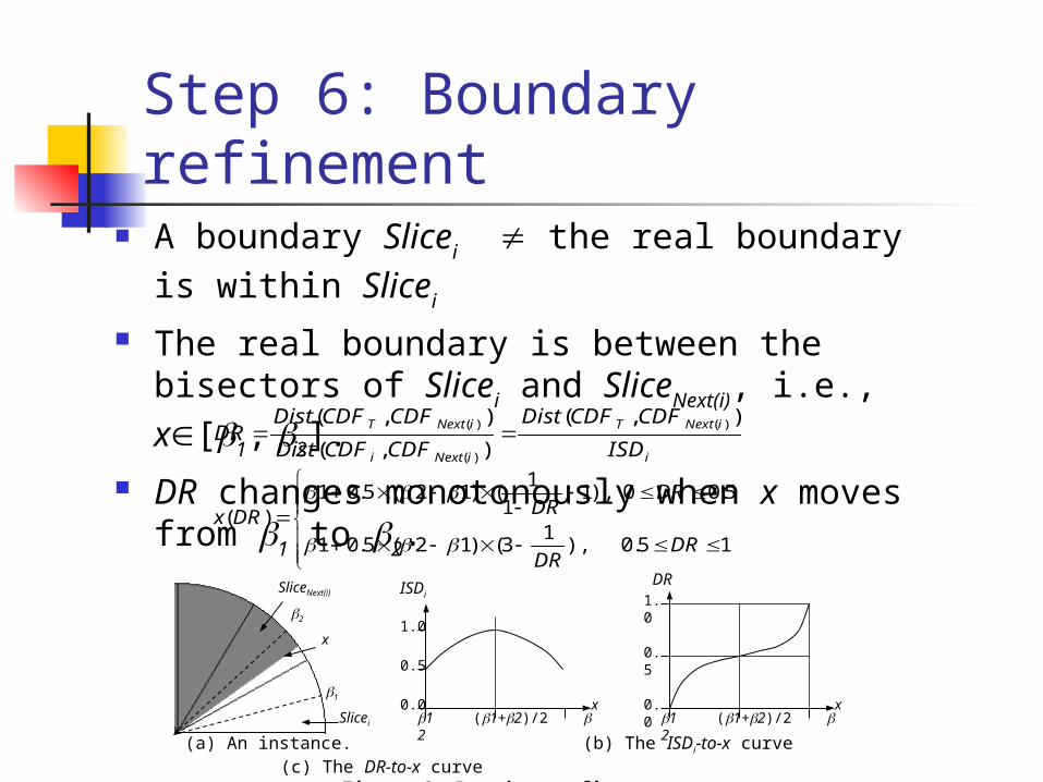
Step 6: Boundary refinement A boundary Slicei the real boundary is within Slicei

The real boundary is between the bisectors of Slicei and

SliceNext(i), i.e., x[1, 2].

DR changes monotonously when x moves from 1 to 2.

(a) An instance. (b) The ISDi-to-x curve (c) The DR-to-x curve

Figure 6. Boundary refinement

SliceNext(i)

Slicei

x

1

2

1 (1+2)/2 20.0

1.0

0.5

ISDi

x1 (1+2)/2 2

0.0

1.0

0.5

DR

x

i

iNextT

iNexti

iNextT

ISD

CDFCDFDist

CDFCDFDist

CDFCDFDistDR

),(

),(

),( )(

)(

)(

15.0),1

3()12(5.01

5.00),11

1()12(5.01

)(

DRDR

DRDRDRx

Step 7: Classification

With the best-divided sectors and their accurate

boundaries, edges, corners and junctions are classified

clearly according to the criteria listed in Table 1.

With the accurate boundary information, the edge strength and the corner strength as follows:

)2,1(' ggDthEdgeStreng

)2,1(' ggDngthCornerStre

Step 8: Localization Directional non-maximal suppression

to localize edges and to eliminate false corners. Regional non-maximal suppression

to localize both corners and junctions. Integrity verification.

to match the branches of corners and junctions with edges.

to eliminate false junctions.

Figure 7. A false corner

P

P2P1Sector1

Sector2

Figure 8: A false junction

M1 M2

V1

V2

O

Implementation techniques Weighting the circular neighborhood.

Rayleigh distribution with a central hole.

CDF is represented by the Color Signature. {(x1,v1), (x2,v2),..., (xn,vn)}, where vi is a vector in a color

space to which the weight xi is assigned.

Dist(CDFi, CDFj) is calculated by the Earth Mover's

Distance (EMD). The saturating distance between two colors (vi and vj) is

calculated by distij =1 - exp{-Eij /14}.

rded

rdorddw d

2,

2,0)(

2

2

2

r 2 0 2 r

Experimental results

Figure 9. Localization accuracy of edge, corner and junction with different .Color description (same for the following figures): red - edge; white - corner; yellow - junction.

(a) Original image. (b) Strength: =2. (c) Strength: =4. (d) Strength: =6. (e) Location: =2.

(f) Location: =4. (g) Location: =6. (h) Boundary: =2. (i) Boundary: =4. (j) Boundary: =6.

Our experiments focus on the localization accuracy, the boundary accuracy, the ability of detecting the junctions with many boundaries, the ability of handling textured regions, and the speed.

Experimental results (cont’d)

(a) Original image (b) Strength (c) Boundaries (d) Original image (e) Strength (f) Boundaries

Figure 10. Detection of 6-region junctions ( = 3).

Figure 11. Edge, corner and junction detection on a textured image

(a) Original image (b) Ours: all features. (c) Compass: edge. (d) Compass: corner.

(e) Compass: junction. (f) SUSAN: edge. (g) SUSAN: corner. (h) Ours: final results.

Experimental results (cont’d)

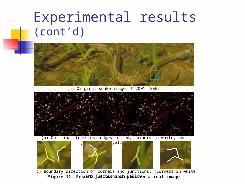
Figure 12. Results of our detector on a real image

(a) Original snake image. © 2001 IEEE.

(b) Our final features: edges in red, corners in white, and junctions in yellow. ( =3)

(c) Boundary direction of corners and junctions. (Corners in white and junctions in yellow)

Experimental results (cont’d)

Table 2 shows their processing time (in seconds) on a 512512 real image with different .

for Compass operator and our detector, the radius of circular neighborhood is 3,

for SUSAN detector, the radius is .

Conclusions Solved the problem of detecting edges, corners and junctions

from color images simultaneously, while handling textured regions.

A generic neighborhood model to classify edges, corners and junctions clearly by their color distributions.

A low-level feature detection approach which is the first one with all the following four capabilities:

detecting edges, corners and junctions in the same pass; handling both uniform-colored regions and textured regions; able to detect free-shaped corners and junctions; producing the accurate boundary direction for corners and junctions.