Engineering Structures 71 (2014) 88–98

Contents lists available at ScienceDirect

Engineering Structures

journal homepage: www.elsevier .com/locate /engstruct

A generic time domain implementation scheme for non-classicalconvolution damping models

http://dx.doi.org/10.1016/j.engstruct.2014.04.0210141-0296/� 2014 Elsevier Ltd. All rights reserved.

⇑ Corresponding author.E-mail address: ama299@uclive.ac.nz (A.M. Puthanpurayil).

Arun M. Puthanpurayil ⇑, Athol J. Carr, Rajesh P. DhakalDepartment of Civil and Natural Resources Engineering, University of Canterbury, Christchurch, New Zealand

a r t i c l e i n f o

Article history:Received 7 May 2013Revised 7 April 2014Accepted 9 April 2014

Keywords:Viscous dampingNon-classical dampingTime-domain formulationNewmark integration

a b s t r a c t

A generic time domain integration formulation for linear systems with non-classical convolutiondamping models is presented. The non-classical damping force is assumed to depend on the past historyof velocity through a convolution integral over a causal dissipative kernel function. The time domainimplementation formulation is developed using the Newmark constant average acceleration framework.To emphasize the accuracy of the proposed scheme, numerical comparisons are made for a three-degrees-of-freedom system and an axially vibrating rod problem reported in literature. The generalityof the formulation is shown by simulating the response of a cantilever beam enhanced with two knownstandard dissipation functions: the exponential and the Gaussian model. The implementation of theproposed scheme is also presented.

� 2014 Elsevier Ltd. All rights reserved.

1. Introduction

Structural dynamic analysis is mainly characterized by threeforces: the inertia force, the damping force and the stiffness force.Out of these, the mechanics for both the inertia and the stiffnessforce are well understood whereas the damping force representsan observed phenomenon. Damping, in simplistic terms, could bedefined as the process by which a certain portion of the energyin a vibrating system is irreversibly lost causing decay in the sys-tem response. Despite having a large amount of literature on thesubject, the underlying physics is only known in a phenomenolog-ical ad hoc manner, making damping an overall mystery in thegeneral dynamic analysis of structures. A major reason of thiscould be the fact that there is no single universally accepted modelfor damping [1]. The ambiguity involved in the modelling ofdamping is mainly due to the intricacies involved in understandingthe state variables controlling the damping forces [2].

In classical dynamics, for a discrete system, the damping force ispredominantly represented by a viscous model, proposed by Ray-leigh in 1877 [3], through his famous dissipation function. This isthe most popular model currently used both in practice and inresearch mainly due to its simplicity, because the whole phenom-enon of damping is mathematically reduced to the estimation of asingle parameter called damping ratio [4]. Many studies in thepast have shown that the viscous damping model suggested by

Rayleigh is only a mathematical idealization and the ‘‘real damp-ing’’ could be different [1,2]. This sort of mathematical idealizationmay lead to ‘‘modelling errors’’ in dynamic response analysis. Themanifestation of these modelling errors has been obtained invarious branches of engineering [5,6]. This has paved the way foran increasing interest in other types of models which representdamping forces in a more general manner as compared to theclassical viscous damping model [7].

One such model of great interest is the non-classical convolu-tion damping model in which the damping force is representedby convolution integrals, which take into account the completepast history of responses other than just the instantaneous veloci-ties as represented by viscous damping model [2,7]. The dampingforce f(t), using such a model could be expressed as,

f ðtÞ ¼Z t

0Ckgðt � sÞ _uðsÞds ð1Þ

In this equation, g(t) represents the damping kernel functionand Ck represents the damping coefficient. The kernel functiong(t) could represent any causal model which makes the energydissipation functional non-negative [8]. Normally, g(t) is taken asthe normalized damping function [9], which satisfies,Z 1

0gðtÞdt ¼ 1:0 ð2Þ

In literature this is commonly referred to as non-viscous damp-ing model [1], considering the fact that integration by parts of Eq.(1) would result in the damping force being expressed as a function

A.M. Puthanpurayil et al. / Engineering Structures 71 (2014) 88–98 89

of displacement. But considering the fact that damping force in itsform as given in Eq. (1) is in a convolution format depending on thepast history of velocities, the authors prefer to address the formu-lation as non-classical convolution damping.

Incorporation of this model described in Eq. (1) into thedynamic equilibrium equation would result in an integro-differen-tial equation expressed as,

Mf€uðtÞg þZ t

0Ckgðt � sÞf _uðsÞgdsþ KfuðtÞg ¼ fPðtÞg ð3Þ

Here, M and K 2 RN�N are the mass and stiffness matrices and{P(t)} 2 RN is the force vector and the convolution damping termhas the same descriptions as defined above in Eq. (1) with Ck rep-resenting the damping coefficient matrix. Similarly f€uðtÞg; f _uðsÞg &

fuðtÞg are the acceleration, velocity and displacement vectors. Theinitial conditions associated with Eq. (3) are as follows,

fuð0Þg ¼ fu0g 2 RN ; and f _uð0Þg ¼ f _u0g 2 RN ð4Þ

As Eq. (3) is an integro-differential equation, no classical meth-ods like Newmark family methods can be applied directly for itssolution [9]. So in recent years, considerable amount of researchefforts have been put to solve Eq. (3) to obtain system responses.The majority of the research conducted presented solutionschemes for systems in which the damping kernel function adoptsan exponential model. McTavish and Hughes [10] adopted the dou-ble exponential model proposed by Golla and Hughes [5] for thedamping kernel function and proposed a scheme which resultedin a second order equation of motion. This second order equationof motion was then solved using classical time integrationtechniques. This scheme is known as the GHM method. Its maindrawback is the use of a large number of internal dissipation coor-dinates used to capture the frequency dependent viscoelasticbehavior which enlarges the matrix size. Adhikari and Wagner[7] proposed a time domain analysis scheme for systems withexponential damping kernel function based on an extended statespace representation of the equation of motion. The efficiency ofthe proposed numerical method for the calculation of displace-ments relies on the elimination of the need for explicit calculationof the velocities and usually a large number of internal variables ateach time step. Cortes et al. [9] employed Laplace transformationon the equation of motion containing exponential damping kernelfunction and derived an equivalent second order equation ofmotion which was then solved using implicit standard time inte-gration schemes. The main advantage of this method was that itdid not employ any internal variables which normally increasedthe size of the problem. The main disadvantage is that the Laplacetransformation results in a differential equation with time deriva-tive orders higher than two and the authors admit the difficulty inperforming the mathematical manipulation, when the dampingmodel has more than two exponential kernel functions.

In this paper, a generic time domain formulation for multi-degree of freedom systems represented by Eq. (3) is presented. Thisis called ‘generic’ because in comparison to majority of the earlierworks, this formulation could be used for any causal model that thedamping kernel function adopts. The other main advantage is thatthe formulation uses the Newmark framework with some modifi-cations and as a result could be easily incorporated into an existingcommercial software package. This aspect has been demonstratedby incorporating the proposed formulation into the commercialpackage ‘‘Ruaumoko’’ maintained by the second author and iscurrently under testing. Latest version of Ruaumoko yet to bereleased gives the option of incorporating convolution dampingmodels for dynamic analysis of structures, though presently it isfully restricted to linear analysis. The implementation logic ispresented in Appendix B.

2. Mathematical derivation

In this section the time domain formulation is developed usingNewmark constant average acceleration frame work. At time t, thedynamic equilibrium equation with linear generic damping modelof the form presented in Eq. (1) is given by Eq. (3).

At time t + DT, this equation becomes,

Mf€uðt þ DTÞg þZ tþDT

0Ckgðt þ DT � sÞf _uðsÞgdsþ Kfuðt þ DTÞg

¼ fPðt þ DTÞg ð5Þ

Here, a revised Newmark constant average acceleration method(rather than the classical incremental approach) is adopted to solvethe equation of equilibrium at time t + DT [11]. The fundamentalassumption in the classical Newmark constant average accelera-tion method is that the acceleration is assumed to be constantduring the time step with a value equal to the average of the accel-erations at the beginning and end of the time step. The classicalNewmark method starts with the difference in the responsebetween two successive time steps DT apart and results in solvingan incremental equilibrium equation. But the revised Newmarkscheme starts with equation of equilibrium at time t + DT (referAppendix A for further details).

In order to have a convenient formulation for the Newmarkimplementation, the convolution integral is split and is given asfollows;

Mf€uðt þ DTÞg þZ t

0Ckgðt þ DT � sÞf _uðsÞgds

þZ tþDT

tCkgðt þ DT � sÞf _uðsÞgdsþ Kfuðt þ DTÞg ¼ fPðt þ DTÞg

ð6Þ

The above equation can be rewritten in incremental terms as(refer Appendix A),

Mf€uðtÞ þ D€ug þZ t

0Ckgðt þ DT � sÞf _uðsÞgds

þZ tþDT

tCkgðt þ DT � sÞf _uðsÞgdsþ KSfuðtÞg þ KTfDug

¼ fPðt þ DTÞg ð7Þ

Here, {Du} refers to increment in displacement, fD€ug refers toincrement in acceleration, KT refers to the tangent stiffness andKS refers to the secant stiffness. For linearly elastic structures, thesecant and tangent stiffness matrices are identical to the initialelastic matrices. Though the present paper addresses only thelinear dynamics scenario, the above notation of secant and tangentstiffness matrix is mainly retained to keep the generality of theNewmark integration scheme. In Eq. (7), both the accelerationand displacement within a time step are represented in theirincremental components, whereas the velocity still remains as acontinuous function. There are two integral terms containingvelocity functions in Eq. (7); one varies from 0 to t and the otherfrom t to t + DT. So, the velocity term varies both globally (i.e. 0to t) and locally (i.e. t to t + DT). Now for convenience, let’s denotethe convolution integral from 0 to t as,

fFdampg ¼Z t

0Ckgðt þ DT � sÞf _uðsÞgds ð8aÞ

So Eq. (7) could be rewritten as,

Mf€uðtÞ þ D€ug þ fFdampg þZ tþDT

tCkgðt þ DT � sÞf _uðsÞgds

þ KSfuðtÞg þ KTfDug ¼ fPðt þ DTÞg ð8bÞ

90 A.M. Puthanpurayil et al. / Engineering Structures 71 (2014) 88–98

In order to simplify the computation process, an assumption ismade on the nature of the local variation of the velocity term (i.e.f _uðsÞg with ‘s’ varying from t to t + DT) which makes numericaldiscretisation of the continuous velocity function f _uðsÞg possiblewithin the time step. As schematically illustrated in Fig. 1, thevelocity is assumed to have a scaled linear variation within a timestep and the function f _uðsÞg is expressed as,

f _uðsÞg ¼ f _uðtÞg þ sDTfD _ug ð9Þ

As it is within the time step, ‘s’ varies from 0 to DT. Note thatthis assumption is mainly based on the classical Newmark’sconstant average acceleration scheme.

Now substituting Eq. (9) in Eq. (8b) and rewriting it by takingthe increments of acceleration, velocity and displacements onone side gives,

MfD€ug þ 1DT

Z tþDT

tCkgðt þ DT � sÞfsD _ugdsþ KTfDug

¼ fPðt þ DTÞg �Mf€uðtÞg � fFdampg � KSfuðtÞg

�Z tþDT

tCkgðt þ DT � sÞf _uðtÞgds ð10Þ

From standard Newmark constant average acceleration method(refer Appendix A), the increments of velocity and acceleration canbe expressed in terms of increments of displacements as,

fD€ug ¼ 4DT2 fDug � 4

DTf _uðtÞg � 2f€uðtÞg ð11Þ

fD _ug ¼ 2DTfDug � 2f _uðtÞg ð12Þ

Now substituting Eqs. (11) and (12) in Eq. (10), we get;

M4

DT2 fDug � 4DTf _uðtÞg � 2f€uðtÞg

� �þ 1

DT

Z tþDT

tCkgðt þ DT � sÞ s 2

DTfDug � 2f _uðtÞg

� �� �ds

þ KTfDug ¼ fPðt þ DTÞg �Mf€uðtÞg � fFdampg � KSfuðtÞg

�Z tþDT

tCkgðt þ DT � sÞf _uðtÞgds ð13Þ

Fig. 1. Illustration of variation of velocity within time step.

Collecting the terms containing increments of displacements onone side we get,

4M

DT2 þ2

DT2

Z tþDT

tCkgðt þ DT � sÞsdsþ KT

� �fDug

¼ fPðt þ DTÞg þM f€uðtÞg þ 4DTf _uðtÞg

� �� fFdampg

� KSfuðtÞg �Z tþDT

tCkgðt þ DT � sÞf _uðtÞgdsþ 2

DT

�Z tþDT

tCkgðt þ DT � sÞsf _uðtÞgds ð14Þ

Eq. (14) represents the final format of the formulation thatneeds to be solved iteratively. A qualitative review of Eq. (14)would reveal the fact that the framework of Newmark is retainedas such with inclusion of damping terms in integral format. Thisenables an easy implementation of the above formulation in exist-ing commercial packages with minor modifications for evaluatingthe integrals. The assumption made in Eq. (9) discretizes the vari-ation of velocity function within a time step and simplifies theevaluation of the integral terms.

3. Implementation strategy

The implementation of the above scheme (Eq. (14)) is simpleand straight forward. For reducing the computational time, thisequation could be used in a semi-discrete form in a numericalsense. This means that wherever velocity is not a function of theintegrating parameter (ds), a closed form solution, if it exists, couldbe used for evaluating the integral. In a semi-discrete format, thewhole of Eq. (14) is as shown below,

4M

DT2 þ2

DT2

Z tþDT

tCkgðt þ DT � sÞsdsþ KT

� �fDug

¼ fPðt þ DTÞg þM f€uðtÞg þ 4DTf _uðtÞg

� ��Xnþ1

r¼1

Ckgððnþ 1

� rÞDTÞf _uðrDTÞgDT � KSfuðtÞg �Z tþDT

tCkgðt þ DT � sÞ

� f _uðtÞgdsþ 2DT

Z tþDT

tCkgðt þ DT � sÞf _uðtÞgsds ð15Þ

Over here the index ‘n’ refers to the number of time steps suchthat t = nDT. So in a semi-discrete form, only one numerical inte-gration is needed to be undertaken as shown by Eq. (15), whereasall other integrations are performed using closed form solutions. Ifclosed form solutions are not available then the full numerical dis-crete format of Eq. (14) could be used and all the integrals could beevaluated using numerical integrations. But this might increase thecomputational time.

In a fully discrete format Eq. (14) becomes,

4M

DT2 þ2

DT2

Xq

p¼0

CkgðnDT þ DT � pDsÞðpDsÞDsþ KT

24 35fDug

¼ fPðt þ DTÞg þM €uðtÞ þ 4 _uðtÞDT

� ��Xnþ1

r¼1

Ckgððnþ 1� rÞDTÞf _uðrDTÞgDT � KSfuðtÞg

�Xq

p¼0

CkgðnDT þ DT � pDsÞf _uðnDTÞgDs

þ 2DT

Xq

p¼0

CkgðnDT þ DT � pDsÞðpDsÞf _uðnDTÞgDs ð16Þ

A.M. Puthanpurayil et al. / Engineering Structures 71 (2014) 88–98 91

Over here, the local variation of the s parameter from t to t + DTis discretised such that DT = qDs. Eq. (16) would require fournumerical integrations per time step which would result in anincrease in the computational time and the response wouldbecome more sensitive to the incremental time step. From a prac-tical computational perspective Eq. (16) might not be a viablescheme. But even with this disadvantage, Eq. (16) represents thegenerality of the above formulation in a mathematical sense. Thesimulations presented in the next sections use the semi-discreteformat presented in Eq. (15). An illustration of the implementationof Eq. (15) is presented in Appendix B.

4. Quantitative comparison with Adhikari and Wagner scheme

In this section, in order to investigate the accuracy of the abovederived method a comparative study is performed using thenumerical results obtained by Adhikari and Wagner [7]. Twonumerical examples were considered in [7]. The two systems stud-ied comprises of a three degrees of freedom system and an axiallyvibrating rod. The convolution damping kernel function for bothsystems adopt double exponential model. These examples werealso used by Cortes et al. [9] to show the accuracy of their method.Interestingly in this paper [9], the plot for the second example(axially vibrating rod) disagreed with the original displacementresponse plotted in the work of Adhikari and Wagner [7] by anorder of 102 which the authors consider a gross conversion error.

4.1. Example 1 (three degrees of freedom system)

The three degrees of freedom system considered by Adhikariand Wagner [7] is shown in Fig. 2.

The equation of motion of the system with double exponentialdamping is given as,

Mf€uðtÞg þZ t

0½l1e�l1ðt�sÞC1 þ l2e�l2ðt�sÞC2�f _uðsÞgdsþ KfuðtÞg

¼ ff ðtÞg ð17Þ

Over here M and K is the mass and stiffness matrices as givenbelow.

M ¼m 0 00 m 00 0 m

264375 ð18Þ

and

K ¼2k �k 0�k 2k �k

0 �k 2k

264375 ð19Þ

where m = 3.0 kg and k = 2.0 N/m.C1 and C2 are the damping coefficient matrices and are given as

below,

Fig. 2. Three DOF model of A

C1 ¼c1 0 00 c1 00 0 0

264375 ð20Þ

C2 ¼0 0 00 c2 �c2

0 �c2 c2

264375 ð21Þ

where c1 = 0.6 N s/m and c2 = 0.2 N s/m. Also, l1 = 1.0 s�1 andl2 = 5.0 s�1 are adopted. The external force vector {f(t)} = 0 andthe initial conditions are given as fu0g ¼ 1 0 0f gT and f _u0g ¼

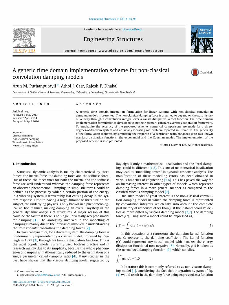
0 0 0f gT . The system response is computed using the methoddescribed in Section 2 and the displacement response at the firstdegree of freedom {u1(t)} is plotted in Fig. 3. The fundamental per-iod of vibration of the system is 10.05 s.

Fig. 3 illustrates the fact that the proposed scheme (denoted asAAR) gives almost the same results as the Adhikari and Wagnermethod (denoted as AW) and the slight discrepancy exhibitedcan be considered to be within practical limits. In the figure, ‘dT’refers to time step DT. It has to be remarked that the proposedmethod requires smaller time steps ðDT 6 0:002 sÞ as comparedto the AW method (DT = 0.02 s); hence more computational time.As the time step increases (DT = 0.01 s), deviation from theexpected response could be observed.

4.2. Example 2 (axial rod problem)

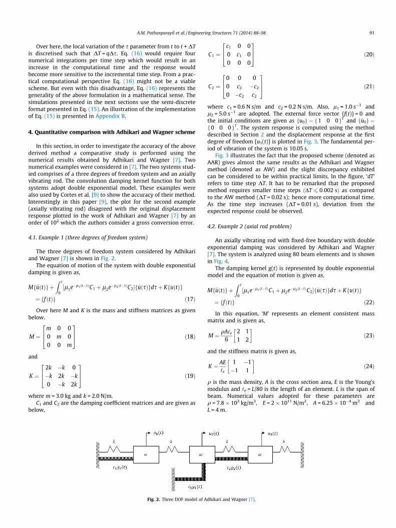
An axially vibrating rod with fixed-free boundary with doubleexponential damping was considered by Adhikari and Wagner[7]. The system is analyzed using 80 beam elements and is shownin Fig. 4.

The damping kernel g(t) is represented by double exponentialmodel and the equation of motion is given as,

Mf€uðtÞg þZ t

0½l1e�l1ðt�sÞC1 þ l2e�l2ðt�sÞC2�f _uðsÞgdsþ KfuðtÞg

¼ ff ðtÞg ð22Þ

In this equation, ‘M’ represents an element consistent massmatrix and is given as,

M ¼ qA‘e

62 11 2

� �ð23Þ

and the stiffness matrix is given as,

K ¼ AE‘e

1 �1�1 1

� �ð24Þ

q is the mass density, A is the cross section area, E is the Young’smodulus and ‘e = L/80 is the length of an element. L is the span ofbeam. Numerical values adopted for these parameters areq = 7.8 � 103 kg/m3, E = 2 � 1011 N/m2, A = 6.25 � 10�4 m2 andL = 4 m.

dhikari and Wagner [7].

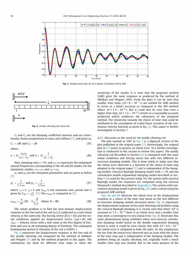
Fig. 3. Displacement plot for first degree of freedom AW & AAR.

Fig. 4. Axially vibrating free fixed rod.

92 A.M. Puthanpurayil et al. / Engineering Structures 71 (2014) 88–98

C1 and C2 are the damping coefficient matrices and are conve-niently chosen proportional to mass and stiffness [7], and given as,

C1 ¼ aM and C2 ¼ bK ð25Þ

where,

a ¼ 2nxixj

xi þxjand b ¼ 2n

1xi þxj

ð26Þ

Here, damping ratio n = 5%, and xi, xj represents the undampednatural frequencies corresponding to the ith and jth modes. For thesimulation studies, xi = x1 and xj = x2.

l1 and l2 are the relaxation parameters and are given as below[7]

l1 ¼1

c1Tminand l2 ¼

1c2Tmin

ð27Þ

where c1 = 1, c2 = 2 and Tmin is the minimum time period and isgiven by Tmin ¼ 2p

xmax[7]. The xmax is computed as [7],

xmax ¼p2Lð2N � 1Þ

ffiffiffiffiEq

swhere N ¼ 80: ð28Þ

The whole problem is to find the time-domain displacementresponse at the free end of the rod {u1(t)} subjected to a unit initialvelocity at the same end. The forcing vector {f(t)} = {0} and the ini-tial conditions applied are displacement vector, {u0} = {0} andf _u0g ¼ velocity vector with a unit value at the first degree of free-dom and zero at all remaining degree of freedoms. The undampedfundamental period of vibration of the rod is 0.0031 s.

Fig. 5 represents the displacement response at the free end ofthe axially vibrating rod computed by the method of Adhikariand Wagner [7] and by the method proposed in this paper. Thesimulations are done for different time steps to show the

sensitivity of the results. It is clear that the proposed method(AAR) gives the same response as produced by the method ofAdhikari and Wagner (AW). From the plots it can be seen thatsmaller time steps (DT = 8 � 10�7 s) are needed for AAR methodto arrive at a better accuracy as compared to the AW methodwhere DT = 1.5 � 10�6 s. But it could also be seen that even ahigher time step, DT = 1.5 � 10�6 s results in a reasonably accurateprediction which reinforces the robustness of the proposedmethod. The sensitivity towards the choice of time step could beattributed to the assumption of scaled linear variation of the con-tinuous velocity function as given in Eq. (9). This aspect is furtherinvestigated in Section 5.

4.2.1. Discussion on the result for the axially vibrating rodThe plot marked as ‘AW’ in Fig. 5 is a digitized version of the

plot published in the original paper [7]. Interestingly, the originalplot in [7] seems to possess an initial error. So a further investiga-tion is conducted in this section to review this aspect. The axiallyvibrating rod described in Section 4.2 is simulated with the sameinitial conditions and forcing vector but with two different in-structure damping models. This is done solely to make sure thatthe initial error observed is a function of the choice of time stepadopted in the original paper [7] and is independent of the damp-ing models. Classical Rayleigh damping model with n = 5% and theconvolution double exponential damping model described in Sec-tion 4.2 is used for the present study. For the system with classicalRayleigh model, the responses are computed using the classicalNewmark’s method described in Appendix A. The system with con-volution damping model is given by Eq. (22) and is solved using theproposed AAR method.

Figs. 6a and 6b illustrate the initial error in the displacementresponse as a choice of the time step based on the two differentin-structure damping models discussed above. Fig. 6a representsthe displacement response of the axial vibrating rod problem usingthe classical Rayleigh damping. It is clearly seen that when ‘DT’ isassumed as 1.5 � 10�6 there is an initial error and a smaller timestep show a convergence to zero initial error. Fig. 6b illustrates thissame phenomenon being exhibited when non-classical convolu-tion damping model based on the double exponential dampingkernel is used. It could be seen clearly that with DT = 4.6 � 10�7

the initial error is mitigated in both the plots. So this emphasizesthe fact that the initial error observed was an issue with the choiceof the time step and is independent of the damping models. Theproblem being an axially vibrating rod, originally itself a muchsmaller time step was needed. But as the main purpose of the

Fig. 5. Response of the free end of the rod AAR & AW.

A.M. Puthanpurayil et al. / Engineering Structures 71 (2014) 88–98 93

simulation in Section 4.2 is to compare the accuracy of the pro-posed formulation with the solutions of Adhikari and Wagner [7],the same ‘DT’ as adopted in the original paper [7] was used forcomparison.

5. Study on the sensitivity of the choice of time step

As shown in Section 4, the time domain responses of the pro-posed method (AAR) is sensitive to the choice of the time step. Afurther investigation is presented in this section using the problemof the axial rod described in Section 4.2, to look into the impact ofthe assumption made in Eq. (9) and how well it approximates thetrue nature of variation of velocity within a time step. First, a largetime step ‘DT’ is selected and then further velocity response anddamping force evaluation is carried out using time steps corre-sponding to DT/2, DT/4, DT/8, and DT/16. Fig. 7 represents the var-iation of the velocity function in an analysis as a choice of timestep. In these plots the initial time step ‘DT’ is assumed to be1.5 � 10�6 s and plotted for a duration of 1.5 � 10�5 s, which isequal to ‘10DT’. From the plot it is clear that the assumption oflinear variation of velocity may not be strictly valid.

Fig. 6a. Illustration of time step e

Fig. 8 further investigates the impact of the assumption in Eq.(9) on the variation of the damping force in an analysis as a choiceof time step. As outlined above, this figure also qualitatively rein-forces the fact illustrated by Fig. 7, that a linear discretisingassumption of velocity might not be strictly valid.

Considering the above observations, it could be argued that abetter discretising assumption would be the use of a quadratic var-iation of velocity within the time step. But this may result in thedemand for more rigorous integrations and different integrationschemes, which in turn may result in making the semi-discrete for-mat presented in Eq. (15) invalid. This would result in a loss of bothefficiency and simplicity of the proposed formulation. So consider-ing all the practical consequences highlighted, and as the presentmethodology is based on Newmark’s constant average accelerationframework, the authors feel that a linear discretisation of thevelocity function is imperative and acceptable.

Reviewing the response calculations in the two examplesdiscussed in the Section 4, it could be concluded that the requiredsmaller time steps are within practical limits and also the use of alarger time step does not result in a large error. So considering themathematical simplicity of the AAR scheme and its ease in imple-menting in a commercial package, an increase in computational

rror with Rayleigh damping.

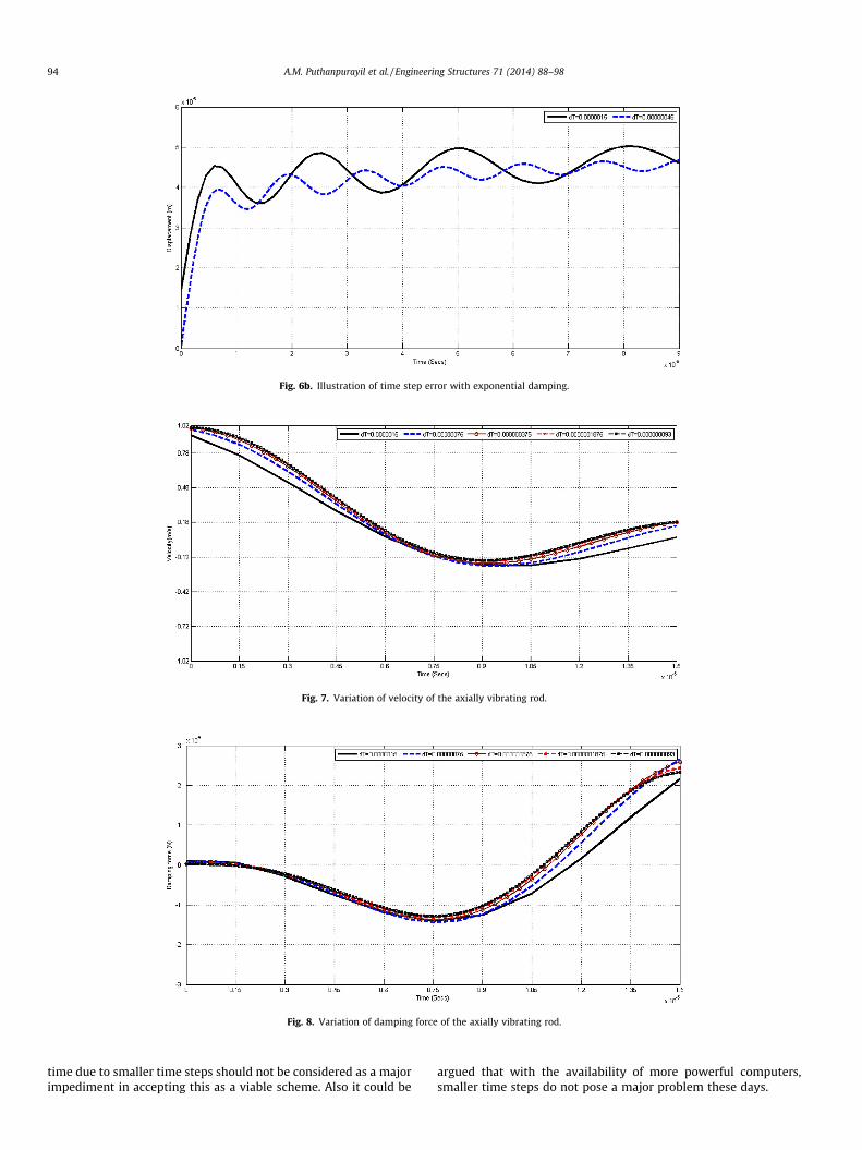
Fig. 6b. Illustration of time step error with exponential damping.

Fig. 7. Variation of velocity of the axially vibrating rod.

Fig. 8. Variation of damping force of the axially vibrating rod.

94 A.M. Puthanpurayil et al. / Engineering Structures 71 (2014) 88–98

time due to smaller time steps should not be considered as a majorimpediment in accepting this as a viable scheme. Also it could be

argued that with the availability of more powerful computers,smaller time steps do not pose a major problem these days.

A.M. Puthanpurayil et al. / Engineering Structures 71 (2014) 88–98 95

6. Simulation studies using single exponential and Gaussianmodels

This section is devoted to demonstrate the generality of the pro-posed AAR scheme by emphasizing the capability to handle differ-ent causal dissipative models which the kernel function g(t)adopts. In order to do that, numerical simulation studies are car-ried out on a cantilever steel beam with kernel dissipative functionof Eq. (1) taking the form of a single exponential and a Gaussiancausative model. The implementation scheme for the AAR methodis given in Appendix B. The main difference in the use of differentmathematical causal models occurs in the evaluation of the closedform integrals in step 3 given in Appendix B (in this particular casethe kernel function g(t) adopts an exponential or Gaussian form).Timoshenko formulation illustrated in Appendix C is used to repre-sent the cantilever beam. A 4 m long cantilever steel beam of100 mm square cross section and subjected to a constant timeindependent transverse point load of 100 N applied at the freeend is adopted for the numerical investigation. Given the describedgeometry an Euler beam could easily have been used for thisnumerical study; but since the numerical technique was developedas part of a bigger project necessitating the use of Timoshenkobeam, it was retained for this numerical study as well. Throughoutthe simulation the applied force is constant so that eventually thesteady state would coincide with the static deflection. Materialproperties adopted are Young’s modulus E = 2 � 1011 N/m2 andmass density q = 7.8 � 103 kg/m3. The system is analyzed using50 beam elements. The equation of motion for the beam with therespective damping kernel functions would be expressed as,

Single Exponential Function

Mf€uðtÞg þZ t

0Ckl1e�l1ðt�sÞf _uðsÞgdsþ KfuðtÞg ¼ ff ðtÞg ð29Þ

Gaussian Function

Mf€uðtÞg þZ t

02

ffiffiffiffiffiffil2

p

re�l2ðt�sÞ

2Ckf _uðsÞgdsþ KfuðtÞg ¼ ff ðtÞg ð30Þ

Here, M, Ck and K represent respectively the mass, dampingcoefficient and stiffness matrices whereas l1 and l2 representrelaxation parameters for the two mathematical causal models.The response evaluations of these two systems are performedusing the formulation described in Section 2. For both systems,the damping coefficient matrix Ck has been conveniently adoptedas proportional to mass and stiffness [7] and is given as,

Ck ¼ aM þ bK ð31Þ

where,

a ¼ 2nxixj

xi þxjand b ¼ 2n

1xi þxj

ð32Þ

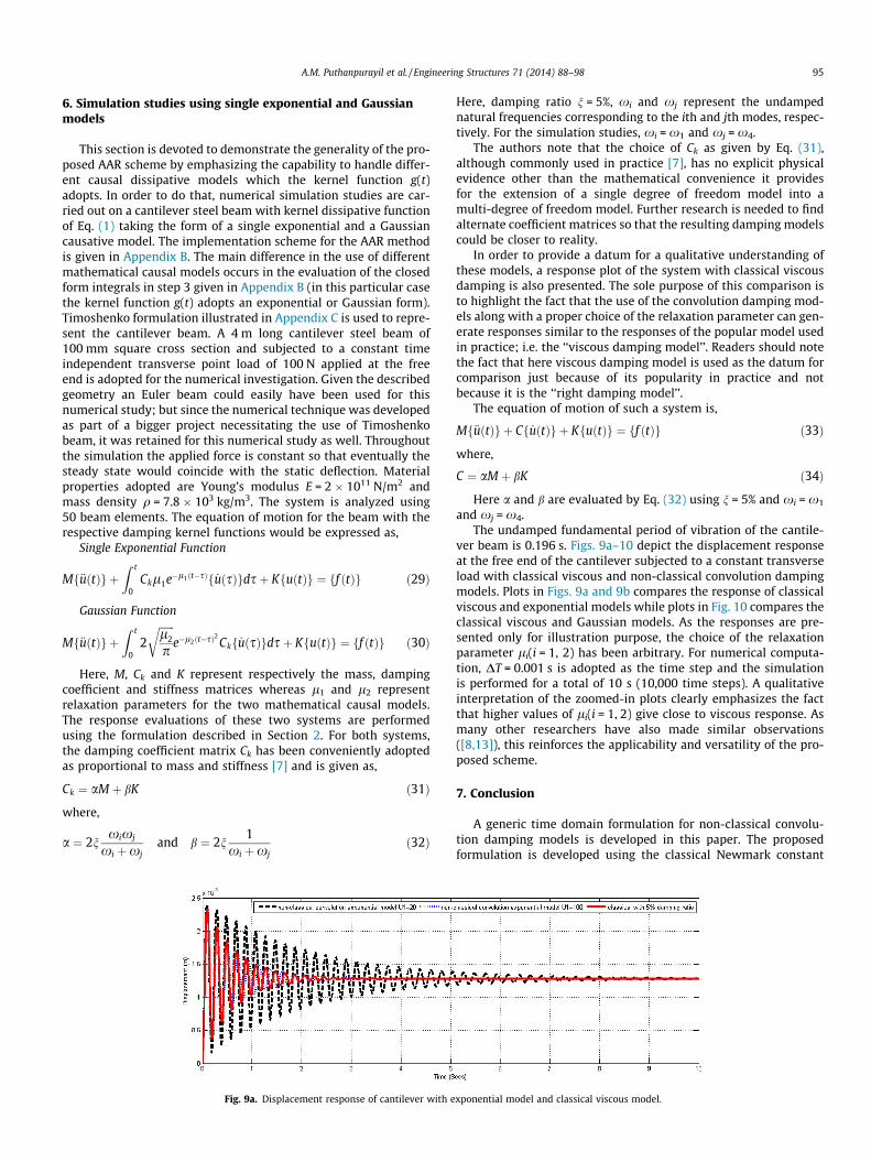
Fig. 9a. Displacement response of cantilever with e

Here, damping ratio n = 5%, xi and xj represent the undampednatural frequencies corresponding to the ith and jth modes, respec-tively. For the simulation studies, xi = x1 and xj = x4.

The authors note that the choice of Ck as given by Eq. (31),although commonly used in practice [7], has no explicit physicalevidence other than the mathematical convenience it providesfor the extension of a single degree of freedom model into amulti-degree of freedom model. Further research is needed to findalternate coefficient matrices so that the resulting damping modelscould be closer to reality.

In order to provide a datum for a qualitative understanding ofthese models, a response plot of the system with classical viscousdamping is also presented. The sole purpose of this comparison isto highlight the fact that the use of the convolution damping mod-els along with a proper choice of the relaxation parameter can gen-erate responses similar to the responses of the popular model usedin practice; i.e. the ‘‘viscous damping model’’. Readers should notethe fact that here viscous damping model is used as the datum forcomparison just because of its popularity in practice and notbecause it is the ‘‘right damping model’’.

The equation of motion of such a system is,

Mf€uðtÞg þ Cf _uðtÞg þ KfuðtÞg ¼ ff ðtÞg ð33Þ

where,

C ¼ aM þ bK ð34Þ

Here a and b are evaluated by Eq. (32) using n = 5% and xi = x1

and xj = x4.The undamped fundamental period of vibration of the cantile-

ver beam is 0.196 s. Figs. 9a–10 depict the displacement responseat the free end of the cantilever subjected to a constant transverseload with classical viscous and non-classical convolution dampingmodels. Plots in Figs. 9a and 9b compares the response of classicalviscous and exponential models while plots in Fig. 10 compares theclassical viscous and Gaussian models. As the responses are pre-sented only for illustration purpose, the choice of the relaxationparameter li(i = 1, 2) has been arbitrary. For numerical computa-tion, DT = 0.001 s is adopted as the time step and the simulationis performed for a total of 10 s (10,000 time steps). A qualitativeinterpretation of the zoomed-in plots clearly emphasizes the factthat higher values of li(i = 1, 2) give close to viscous response. Asmany other researchers have also made similar observations([8,13]), this reinforces the applicability and versatility of the pro-posed scheme.

7. Conclusion

A generic time domain formulation for non-classical convolu-tion damping models is developed in this paper. The proposedformulation is developed using the classical Newmark constant

xponential model and classical viscous model.

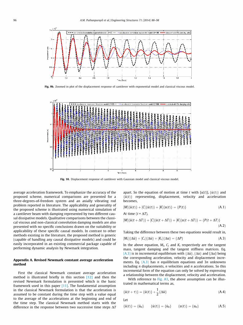
Fig. 9b. Zoomed in plot of the displacement response of cantilever with exponential model and classical viscous model.

Fig. 10. Displacement response of cantilever with Gaussian model and classical viscous model.

96 A.M. Puthanpurayil et al. / Engineering Structures 71 (2014) 88–98

average acceleration framework. To emphasize the accuracy of theproposed scheme, numerical comparisons are presented for athree-degrees-of-freedom system and an axially vibrating rodproblem reported in literature. The applicability and generality ofthe proposed scheme is illustrated using numerical simulation ofa cantilever beam with damping represented by two different cau-sal dissipative models. Qualitative comparisons between the classi-cal viscous and non-classical convolution damping models are alsopresented with no specific conclusions drawn on the suitability orapplicability of these specific causal models. In contrast to othermethods existing in the literature, the proposed method is generic(capable of handling any causal dissipative models) and could beeasily incorporated in an existing commercial package capable ofperforming dynamic analysis by Newmark integration.

Appendix A. Revised Newmark constant average accelerationmethod

First the classical Newmark constant average accelerationmethod is illustrated briefly in this section [12] and then therevised Newmark formulation is presented which is the basicframework used in this paper [11]. The fundamental assumptionin the classical Newmark formulation is that the acceleration isassumed to be constant during the time step with a value equalto the average of the accelerations at the beginning and end ofthe time step. The classical Newmark method starts with thedifference in the response between two successive time steps DT

apart. So the equation of motion at time t with {u(t)}, f _uðtÞg andf€uðtÞg representing, displacement, velocity and accelerationbecomes,

½M�f€uðtÞg þ ½C�f _uðtÞg þ ½K�fuðtÞg ¼ fPðtÞg ðA:1Þ

At time (t + DT),

½M�f€uðt þ DTÞg þ ½C�f _uðt þ DTÞg þ ½K�fuðt þ DTÞg ¼ fPðt þ DTÞgðA:2Þ

Taking the difference between these two equations would result in,

½Mt �fD€ug þ ½Ct�fD _ug þ ½Kt�fDug ¼ fDPg ðA:3Þ

In the above equation, Mt, Ct and Kt respectively are the tangentmass, tangent damping and the tangent stiffness matrices. Eq.(A.3) is in incremental equilibrium with fD€ug; fD _ug and {Du} beingthe corresponding acceleration, velocity and displacement incre-ments. Eq. (A.3) has n equilibrium equations and 3n unknownsincluding n displacements, n velocities and n accelerations. So thisincremental form of the equation can only be solved by expressinga relationship between the displacement, velocity and acceleration.

With reference to Fig. A1, the above assumption can be illus-trated in mathematical terms as,

f€uðt þ sÞg ¼ f€uðtÞg þ 12fD€ug ðA:4Þ

Let

f€uðtÞg ¼ f€u0g f _uðtÞg ¼ f _u0g fuðtÞg ¼ fu0g ðA:5Þ

Fig. A1. Illustration of the variation of the acceleration within a time step inconstant average acceleration method.

A.M. Puthanpurayil et al. / Engineering Structures 71 (2014) 88–98 97

Then Eq. (A.4) can be rewritten as,

f€uðt þ sÞg ¼ f€u0g þ12fD€ug ðA:6Þ

Integrating with respect to s, we get,

f _uðt þ sÞg ¼ f _u0g þ sf€u0g þs2fD€ug ðA:7Þ

and integrating again,

fuðt þ sÞg ¼ fu0g þ sf _u0g þs2

2f€u0g þ

s2

4fD€ug ðA:8Þ

Now at the end of the time step, the velocity and displacement interms of increments of acceleration is given as,

f _uðt þ DTÞg ¼ f _u0g þ DTf€u0g þDT2fD€ug ðA:9Þ

fuðt þ DTÞg ¼ fu0g þ DTf _u0g þðDTÞ2

2f€u0g þ

ðDTÞ2

4fD€ug ðA:10Þ

The increments of velocity and displacement expressed in terms ofincrements of acceleration in Eqs. (A.9) and (A.10) are as follows,

fD _ug ¼ DTf€u0g þDT2fD€ug ðA:11Þ

fDug ¼ DTf _u0g þðDTÞ2

2f€u0g þ

ðDTÞ2

4fD€ug ðA:12Þ

Now rearranging the above equations in terms of increments of dis-placement results in,

fD€ug ¼ 4DT2 fDug � 4

DTf _uðtÞg � 2f€uðtÞg ðA:13Þ

fD _ug ¼ 2DTfDug � 2f _uðtÞg ðA:14Þ

The revised Newmark scheme starts with equation of equilibrium attime t + DT,

½M�f€uðt þ DTÞg þ ½C�f _uðt þ DTÞg þ ½K�fuðt þ DTÞg ¼ fPðt þ DTÞgðA:15Þ

The following relations are used for the development of the scheme,

½Kðt þ DTÞ�fuðt þ DTÞg ¼ ½KðtÞ�fuðtÞg þ ½Kt �fDug ðA:16Þ

½Cðt þ DTÞ�f _uðt þ DTÞg ¼ ½CðtÞ�f _uðtÞg þ ½Ct �fD _ug ðA:17Þ

½Mðt þ DTÞ�f€uðt þ DTÞg ¼ ½MðtÞ�f€uðtÞg þ ½Mt �fD€ug ðA:18Þ

where Kt, Ct and Mt are the corresponding tangent stiffness, tangentdamping and tangent mass matrices and K(t), C(t) and M(t) are thecorresponding secant stiffness, secant damping and secant massmatrices. In the further development of the method these secantmatrices are denoted as M, C and K. Now substituting the aboveequations, (A.16)–(A.18) in (A.15) gives,

½M�f€uðtÞg þ ½Mt �fD€ug þ ½C�f _uðtÞg þ ½Ct �fD _ug þ ½K�fuðtÞg þ ½Kt �fDug¼ fPðt þ DTÞg ðA:19Þ

Now collecting the increment terms on one side,

½Mt �fD€ug þ ½Ct �fD _ug þ ½Kt�fDug¼ fPðt þ DTÞg � ½M�f€uðtÞg � ½C�f _uðtÞg � ½K�fuðtÞg ðA:20Þ

Now by using Eqs. (A.13) and (A.14), the increments of accelerationand velocity can be expressed in terms of increments of displace-ment and finally the equilibrium can be written as,

½bK t �fDug ¼ fPðt þ DTÞg þ ½M� f€uðtÞg þ 4DTf _uðtÞg

� �þ 2½Ct�

� f _uðtÞg � ½C�f _uðtÞg � ½K�fuðtÞg ðA:21Þ

where dynamic or augmented stiffness ½bK t� is given as,

½bK t � ¼4

DT2 ½Mt � þ2

DT½Ct� þ ½Kt� ðA:22Þ

Appendix B. Algorithm for implementation of the AAR method

The implementation is carried out using Eq. (15) in most caseswhere a closed form solution as described in Section 3 exists forthe integrals containing the kernel function. Here, the implementa-tion strategy is illustrated for the generic case in which thedamping kernel function g(t) adopts any causal dissipative model.For the generic case, the equation of motion is given as,

Mf€uðtÞg þZ t

0Ckgðt � sÞf _uðsÞgdsþ KfuðtÞg ¼ fPðtÞg ðB:1Þ

The initial conditions are as specified in Eq. (4). Now, the implemen-tation using Eq. (15) involves the evaluation of two integrals inclose form.

B.1. Steps involved in the algorithm

1. Initialise the displacement vector dold = {d0} = {u(0)} and veloc-ity vector vold ¼ fv0g ¼ f _uð0Þg

2. To evaluate initial acceleration consider Eq. (B.1) and we get,

f€uðtÞg ¼ M�1 fPðtÞg �Z t

0Ckgðt � sÞf _uðsÞgds� KfuðtÞg

� �ðB:2Þ

t = 0,

f€uð0Þg ¼ M�1ffPð0Þg �Z 0

0Ckgð0� 0Þf _uð0Þgds� Kfuð0Þgg

ðB:3Þ

aold ¼ f€uð0Þg ¼ M�1 Pð0Þ � Ckgð0Þvold � Kdoldf g ðB:4Þ

98 A.M. Puthanpurayil et al. / Engineering Structures 71 (2014) 88–98

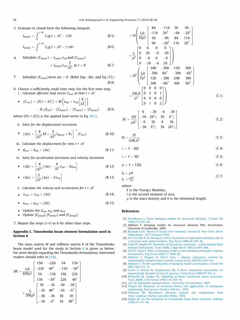
3. Evaluate in closed form the following integrals

5.

�

Idamp1 ¼Z tþDT

tCkgðt þ DT � sÞds ðB:5Þ

Idamp2 ¼Z tþDT

tCkgðt þ DT � sÞsds ðB:6Þ

Initialise fFdamp1g ¼ Idamp1vold andfFdamp2g

¼ Idamp2vold2

DTat t ¼ 0 ðB:7Þ

4.

Initialise fFdampg term at t ¼ 0 ðRefer Eqs: ð8aÞ and Eq:ð15ÞÞðB:8Þ

6. Choose a sufficiently small time step. For the first time step,i. Calculate effective load vector Fnew at time t + DT

fFnewg ¼ fPðt þ DTÞg þM aold þ vold4

DT

� �� �� Ksfdoldg � fFdamp1g � fFdampg þ fFdamp2g ðB:9Þ

where {P(t + DT)} is the applied load vector in Eq. (B.1).

ii. Solve for the displacement increment,

fDug ¼ 4DT2 M þ 2

DT2 Idamp2 þ KT

� ��1

fFnewg ðB:10Þ

�

iii. Calculate the displacement for time t + DT

dnew ¼ dold þ fDug ðB:11Þ

�

iv. Solve for acceleration increment and velocity increment

fD€ug ¼ 4DT2 fDug � 4

DTvold � 2aold

� �ðB:12Þ

�

fD _ug ¼ 2DTfDug � 2vold

� �ðB:13Þ

�

v. Calculate the velocity and acceleration for t + DT

vnew ¼ vold þ fD _ug ðB:14Þ

�

anew ¼ aold þ fD€ug ðB:15Þ

�

� Update the dold, vold and aold

� Update {Fdamp}, {Fdamp1} and {Fdamp2}

7. Repeat the steps (i–v) in 6 for other time steps.

Appendix C. Timoshenko beam element formulation used inSection 6

The mass matrix M and stiffness matrix K of the Timoshenkobeam model used for the study in Section 6 is given as below.For more details regarding the Timoshenko formulation, interestedreaders should refer to [14].

½M� ¼ I0h420l2

156 �22h 54 13h

�22h 4h2 �13h �3h2

54 �13h 156 22h

13h �3h2 22h 4h2

266664377775

þ I2

30hl2

36 �3h �36 �3h

�3h 4h2 �3h �h2

�36 �3h 36 3h

�3h �h2 3h 4h2

266664377775

þXI0h

10l2

84 �11h 36 9h

�11h 2h2 �9h �2h2

36 �9h 84 11h

9h �2h2 11h 2h2

2666437775

0BBB@

þ I2

l2

0 6 0 66 2h �6 �2h0 �6 0 �66 �2h �6 2h

26664377751CCCA

þX2 I0h5l2

240 �30h 120 30h

�30h 6h2 �30h �6h2

120 �30h 240 30h30h �6h2 30h 6h2

2666437775

0BBB@

þ24I2hl2

0 0 0 00 2 0 10 0 0 00 1 0 2

26664377751CCCA ðC:1Þ

½K� ¼ 2EI

lh3

6 �3h �6 �3h

�3h 2h2k 3h h2n

�6 3h 6 3h

�3h h2n 3h 2h2k

2666437775 ðC:2Þ

X ¼ EI

GAKsh2 ðC:3Þ

n ¼ 1� 6X ðC:4Þ

k ¼ 1þ 3X ðC:5Þ

l ¼ 1þ 12X ðC:6Þ

I0 ¼ qA

I2 ¼ qAh2

12

ðC:7Þ

whereE is the Young’s Modulus,

I is the second moment of area,q is the mass density and h is the elemental length.

References

[1] Woodhouse J. Linear damping models for structural vibration. J Sound Vib1998;215:547–69.

[2] Adhikari S. Damping models for structural vibration PhD. Dissertation,University of Cambridge; 2000.

[3] Rayleigh Lord. Theory of Sound (two volumes). second ed. New York: DoverPublications; 1877(reissued 1945).

[4] Lee S-H, Min K-W, Hwang J-S, Kim J. Evaluation of equivalent damping ratio ofa structure with added dampers. Eng Struct 2004;26:335–46.

[5] Golla DF, Hughes PC. Dynamics of viscoelastic structures – a time domain finiteelement formulation. Trans ASME, J Appl Mech 1985;52:897–906.

[6] Val VD, Segal F. Effect of damping model on pre-yielding earthquake responseof structures. Eng Struct 2005;27:1968–80.

[7] Adhikari S, Wagner N. Direct time – domain integration method forexponentially damped linear systems. Comp Struct 2004;82:2453–61.

[8] Adhikari S. On the quantification of damping model uncertainity. J Sound Vib2007;306:153–71.

[9] Cortes F, Mateos M, Elejabarriata MJ. A direct integration formulation forexponentially damped structural systems. Comp Struct 2009;87:391–4.

[10] McTavish DJ, Hughes PC. Modeling of linear viscoelastic space structures.Trans ASME, J Vib Acoust 1993;115:103–10.

[11] Carr AJ. Ruaumoko manual-theory. University of Canterbury; 2007.[12] Chopra AK. Dynamics of structures-theory and applications to earthquake

engineering. New Jersey: Prentice Hall Inc.; 1995.[13] Newland DE. Mechanical vibration analysis and computation. New

York: Longman, Harlow and John Wiley; 1989.[14] Reddy JN. On the behaviour of Timoshenko beam finite elements. Sadhana

1999;24:175–98.