A GEOMETRIC STUDY OF LIQUID RETENTION IN OPEN-CELL METAL FOAMS

BY

JESSICA J. BOCK

THESIS

Submitted in partial fulfillment of the requirements

for the degree of Master of Science in Mechanical Engineering

in the Graduate College of the

University of Illinois at Urbana-Champaign, 2011

Urbana, Illinois

Adviser:

Professor Anthony M. Jacobi

ii

Abstract

Open-cell metal foams show promise as an emerging novel material for heat exchanger

applications. The high surface-area-to-volume ratio suggests increased compactness and decrease

in weight of heat exchanger designs. However, the metal foam structure appears conducive to

condensate retention, which would degenerate heat transfer performance. This research

investigates the condensate retention behavior of aluminum open-cell metal foams through the

use of static dip tests and geometrical classification via X-ray Micro-Computed Tomography.

Aluminum open-cell metal foam samples of 5, 10, 20, and 40 pores per inch (PPI), all having a

void fraction greater than 90%, were included in this investigation.

In order to model the condensate retention behavior of metal foams, a clearer understanding of

the geometry was required. After exploring the ideal geometries presented in the open literature,

X-ray Micro-Computed Tomography was employed to classify the actual geometry of the metal

foam samples. The images obtained were analyzed using specialized software from which

geometric information including strut length and pore shapes were extracted. The results

discerned a high variability in ligament length, as well as features supporting the ideal geometry

known as the Weaire-Phelan unit cell.

The static dip tests consisted of submerging the metal foam samples in a liquid, then allowing

gravity-induced drainage until steady-state was reached and the liquid remaining in the metal

foam sample was measured. Three different liquids, water, ethylene glycol, and 91% isopropyl

alcohol, were employed. The behaviors of untreated samples were compared to samples

subjected to a Beomite surface treatment process, and no significant differences in retention

behavior were discovered. The dip test results revealed two distinct regions of condensate

retention, each holding approximately half of the total liquid retained by the sample. As

expected, condensate retention increased as the pores sizes decreased.

A model based on surface tension was developed to predict the condensate retention in the metal

foam samples and verified using a regular mesh. Applying the model to both the ideal and actual

metal foam geometries showed good agreement with the dip test results in this study.

iii

Acknowledgements

The author would like to thank Professor Anthony Jacobi for his assistance, guidance, and advice

throughout this research; the Air Conditioning and Refrigeration Center at the University of

Illinois for its support of the project; the Air Conditioning, Heating and Refrigeration Technology

Institute (AHRTI) for funding this research; Lei Lei Yin from the Beckman Institute for his

assistance with the X-ray computed tomography; M. D. Montminy for FoamView© support;

Bob Coverdill for assistance with the rapid prototyping; colleagues Kashif Nawaz and Zhengshu

Dia for their valuable discussions on the topic; and family, friends, and Nathan, especially, for

their support and encouragement.

iv

Table of Contents

List of Figures ........................................................................................................................ vi

List of Tables ....................................................................................................................... viii

Nomenclature ........................................................................................................................ ix

Chapter 1: Introduction ........................................................................................................ 1

Chapter 2: Geometric Classification of Open-Cell Metal Foams ...................................... 3

2.1 Background and Literature Review ....................................................................... 3

2.2 X-ray Computed Tomography ............................................................................... 5

2.3 Experimental Methods ........................................................................................... 6

2.4 Analytical Methods ................................................................................................ 8

2.5 Experimental Results ........................................................................................... 10

2.6 Discussion and Conclusions ................................................................................ 29

Chapter 3: Liquid Retention Behavior of Open-Cell Metal Foams ............................... 31

3.1 Background and Literature Review ..................................................................... 31

3.2 Experimental Methods ......................................................................................... 32

3.3 Experimental Results ........................................................................................... 34

3.4 Discussion and Conclusions ................................................................................ 52

Chapter 4: Modeling of Liquid Retention in Open-Cell Metal Foams ........................... 54

4.1 Model Formulation .............................................................................................. 54

4.2 Model Applied to Real Geometry from X-ray CT Data ...................................... 56

4.3 Applied to Ideal Geometry from Weaire-Phelan Unit Cell ................................. 60

4.4 Discussion and Conclusions ................................................................................ 64

Chapter 5: Summary ........................................................................................................... 65

References ............................................................................................................................. 66

Appendix A: Experimental Results: Dip Test Raw Data—Water .................................. 73

Appendix B: Experimental Results: Dip Test Raw Data—Ethylene Glycol .................. 81

Appendix C: Experimental Results: Dip Test Raw Data—91% Isopropyl Alcohol ..... 85

Appendix D: X-ray μCT Image Analysis—Strut Density ................................................ 88

Appendix E: X-ray μCT Image Analysis—Strut Diameter ........................................... 106

Appendix F: Uncertainty Analysis .................................................................................. 110

v

Appendix G: FoamView Reports .................................................................................... 112

Author’s Biography ........................................................................................................... 115

vi

List of Figures

Figure 1.1.a: Image of open-cell aluminum metal foam .......................................................... 1

Figure 1.1.b: Image of closed-cell aluminum metal foam ....................................................... 1

Figure 2.1: Kelvin unit cell ...................................................................................................... 3

Figure 2.2: Weaire-Phelan unit cell ......................................................................................... 4

Figure 2.3: Xradia Bio MicroCT experimental apparatus ....................................................... 7

Figure 2.4: Schematic of X-ray μCT process .......................................................................... 8

Figure 2.5: Radiograph (raw data), 10 PPI ............................................................................ 11

Figure 2.6: Inverted radiograph, 10 PPI................................................................................. 12

Figure 2.7: Radiograph with thresholding, 5 PPI .................................................................. 12

Figure 2.8: Inverted radiograph with thresholding, 5 PPI ..................................................... 13

Figure 2.9: 3D rendering of X-ray CT data, 5 PPI ................................................................. 14

Figure 2.10: Radiographs with triangular cross-sections circled, 5 PPI ................................ 15

Figure 2.11: Determining strut density from radiographs, 10 PPI ......................................... 16

Figure 2.12: Determining strut diameter from radiographs, 10 PPI ...................................... 17

Figure 2.13: Strut diameter determined from X-ray μCT vs. foam PPI ................................ 18

Figure 2.14: MFG Data Diameter .......................................................................................... 19

Figure 2.15: Foamview volume rendering, 10 PPI ................................................................ 20

Figure 2.16: Foamview surface rendering, 10 PPI ................................................................ 21

Figure 2.17: Foamview-generated crude stick figure, 10 PPI ............................................... 22

Figure 2.18: Foamview completed stick figure, 10 PPI......................................................... 22

Figure 2.19: Foamview interface showing completed stick figure, 10ppi ............................. 23

Figure 2.20: Foamview interface showing completed stick figure, 5ppi ............................... 24

Figure 2.21: Foamview histograms, 20 PPI ........................................................................... 25

Figure 2.22: Foamview report window, 20 PPI ..................................................................... 26

Figure 2.23: Strut length distribution ..................................................................................... 27

Figure 2.24: Window shape distribution ................................................................................ 28

Figure 3.1: Open-cell aluminum metal foams of varying foam PPI ...................................... 32

Figure 3.2: Diagram of water retention behavior ................................................................... 33

Figure 3.3: Void fraction vs. foam PPI .................................................................................. 35

vii

Figure 3.4: Total water retained in untreated samples vs. foam PPI ..................................... 36

Figure 3.5: Total water retained in treated samples vs. foam PPI ......................................... 37

Figure 3.6: Total water retained in untreated samples vs. void fraction ................................ 38

Figure 3.7: Total water retained in treated samples vs. void fraction .................................... 39

Figure 3.8: Water retention regions ....................................................................................... 40

Figure 3.9: Percent mass of water retained in the saturated region vs. foam PPI .................. 42

Figure 3.10: Percent volume occupied by liquid in the unsaturated region of

untreated samples vs. foam PPI ................................................................ 43

Figure 3.11: Percent volume occupied by liquid in the unsaturated region of

treated samples vs. foam PPI .................................................................... 44

Figure 3.12: Percent volume occupied by liquid in the unsaturated region of

untreated samples vs. void fraction ........................................................... 45

Figure 3.13: Percent volume occupied by liquid in the unsaturated region of

treated samples vs. void fraction ............................................................... 46

Figure 3.14: Mass of ethylene glycol retained vs. foam PPI ................................................. 48

Figure 3.15: Mass of 91% isopropyl alcohol retained vs. foam PPI ...................................... 49

Figure 3.16: Summary of percent mass of liquid retained in the saturated region ................ 50

Figure 3.17: Summary of percent volume occupied by liquid in the unsaturated

region vs. foam PPI ................................................................................. 51

Figure 3.18: Summary of total mass of liquid retained vs. foam PPI .................................... 52

Figure 4.1: Image of regular mesh rapid prototype ............................................................... 54

Figure 4.2: Model predictions for water using X-ray μCT geometry data ............................ 57

Figure 4.3: Model predictions for 91% IPA using X-ray μCT geometry data ...................... 58

Figure 4.4: Model predictions for ethylene glycol using X-ray μCT geometry data ............ 59

Figure 4.5a: WP unit cell – Struts contributing to surface tension, orientation #1 ................ 60

Figure 4.5b: WP unit cell – Struts contributing to surface tension, orientation #2................ 60

Figure 4.6: Model predictions for WP unit cell compared to dip test results ........................ 63

Figure 4.7: Recently proposed p42a unit cell ........................................................................ 64

viii

List of Tables

Table 2.1: Average strut density determined from X-ray μCT data ...................................... 16

Table 2.2: Average strut diameters determined from X-ray μCT data compared to

data provided by the manufacturer .............................................................. 19

Table 2.3: Summary of strut geometry from X-ray μCT data .............................................. 27

Table 2.4: Window shape distribution from X-ray μCT data compared to ideal

unit cells. ...................................................................................................... 29

Table 3.1: Capillary lengths for three fluids .......................................................................... 47

Table 3.2: Characteristic lengths of metal foam samples ...................................................... 47

Table 4.1: Regular mesh rapid prototype dimensions ........................................................... 55

Table 4.2: Results of prototype dip tests - model validation ................................................. 56

ix

Nomenclature

Ac cross-sectional area of metal foam sample

dctc distance from center of window face to center of pore

standard deviation

g acceleration due to gravity

h height of liquid column retained in metal foam sample

IPQ Isoperimetric quotient

l strut length

L contact length

λc capillary length

m mass

σ surface tension of liquid

void fraction

density

V volume

W weight

Z standard normal Z-factor

Subscripts

avg average

calc calculated from height measurements, h, taken from dip test data

f aluminum metal foam

i at the liquid-vapor interface

liq liquid

LK Lord Kelvin ideal unit cell model

max maximum

pentagon pentagonal window of unit cell

pent-pyramid pentagonal pyramid

req contact length required to hold the liquid mass found in dip tests

tot total volume of foam sample as if it were solid block

unit ideal unit cell geometry

wet metal foam sample with retained water

WP Weaire-Phelan ideal unit cell model

X-ray obtained from X-ray μCT data

1

Chapter 1: Introduction

In order to successfully use a new material, it is critical to understand its properties and its

interactions with other materials. Metal foams are relatively new materials that show promise in

a range of fields [1-3]. There are varieties of metal foams available, as well as means of

producing them [4-9]. Metal foams can generally be described by a few key features: the base

material is perhaps the most obvious descriptor. Metal foams are currently being produced from

aluminum, copper, brass, and steel, among other metals. The research described here focuses on

aluminum (Al-6101-T6) metal foams. The other main feature is the foam structure. Metal foams

are being produced as open-cell and closed-cell foams. An open-cell metal foam consists of

pores that are open to their neighboring pores. The closed-cell metal foams have a thin layer of

metal dividing the individual pores. The differences are easily seen, as shown in Figure 1.1. This

research will be restricted to open-cell metal foams. In addition to material and cell structure,

metal foam is generally classified by the number of pores per inch (PPI), which is a measurement

of pore density. Foam PPI is the main method of classification amongst metal foams of the same

material and cell structure.

Figure 1.1[71]

: Image of (a) open-cell and (b) closed-cell aluminum metal foam

Open-cell metal foams look particularly promising as a novel material for heat exchanger

applications [10-17]. The high surface-area-to-volume ratio shows promise for increased

compactness and decrease in weight of heat exchangers. Numerous researchers have been

2

interested in the thermal and hydraulic performance of metal foams, and several models are

available in the literature [18-26].

An increasing concern in heat exchanger design and performance is condensation retention [27-

31]. The effects of condensate retention on heat exchanger performance has been studied, and

new methods of improving condensate shedding are being developed [32, 33]. As metal foam is

a relatively new material, little is known about its condensate retention behavior

This research focuses on the validity of geometric models for open cell metal foams. Idealized

geometric models are compared to geometric data obtained from an X-ray micro-CT analysis.

The geometric information is compared to experimentally obtained data regarding the liquid

retention of three fluids in metal foams. The real and ideal geometries are compared to a model

of the liquid retention behavior of metal foams, which may be valuable in heat exchanger design.

The results provide a means for estimating liquid retention and recommend the ideal geometric

model which most accurately represents metal foam structures. The metal foam samples used in

this research were Duocel® Al-6101-T6 open-cell foams from ERG.

3

Chapter 2: Geometric Classification of Open-Cell Metal Foams

2.1 Background and Literature Review

The problem of finding the geometrical structure for foams has a long history. In 1887 Lord

Kelvin proposed a solution to what has become known as „the Kelvin problem‟ [34]. The search

for a unit cell that partitions three-dimensional space with minimal surface area has spurred

many publications by mathematicians and physicists [34-46]. The ideal geometry of metal foam

has been connected to the geometry of bubbles, soapy froths, and wet foams. In this body of

literature, an increasing number of foam descriptions can be found [47-55]. The Kelvin unit cell

is one of two predominant descriptions of ideal geometry.

Kelvin conjectured that the tetrakaidecahedron satisfied the requirements of a space-filling

polyhedron that models an arrangement of cells of equal volume and minimum surface area. The

tetrakaidecahedron consists of six square and eight hexagonal faces, and is bounded by Plateau‟s

rules for equilibrium structures [56]. The Kelvin unit cell, shown in Figure 2.1, can also be seen

as a body-centered-cubic (bcc) structure with slightly curved faces, which allow the cell to

satisfy Plateau‟s rules.

Figure 2.1: Kelvin unit cell

“This problem is solved in foam,” according to Kelvin, and has been accepted as the ideal unit

cell for more than a century. While widely accepted, the Kelvin conjecture had yet to be proven

or disproven and the often cited experiments and observations by the botanist Matzke (1946)

[57] failed to reveal this structure in natural forms.

4

After more than a century of Kelvin‟s conjecture going uncontested, Weaire and Phelan

introduced a counter-example that succeeded in reducing the surface energy [37]. This new unit

cell consisted of multiple, irregular polyhedral of equal volume. The Weaire-Phelan (WP) unit

cell consists of six 14-sided polyhedra and two 12-sided polyhedral, as shown in Figure 2.2. It

was derived from a tetrahedrally-close-packed (tcp) structure, a family of structures that are

commonly observed in chemical clathrates [40] and was optimized using the “Surface Evolver”

package of Brakke [58] to determine the curvature required to minimize surface area. With

advances in technology, such as the Surface Evolver software, increasingly complicated unit

cells can be analyzed in pursuit of the optimum solution to the Kelvin problem. [41]

Figure 2.2[59]

: Weaire-Phelan unit cell

The isoperimetric quotient, IPQ, is a figure of merit for area minimization defined in equation

2.1, where Vunit and Aunit are the volume and surface area of a single unit cell, respectively.

Although the WP unit cell improved the IPQ by approximately 0.3% as compared to the Kelvin

unit cell, the model is still just a conjecture.

2

3

36 unit

unit

VIPQ

A

(2.1)

5

It is important to note that although the WP unit cell has pores of equal volume, they are not of

equal pressure, where pore pressure and volume are based on a soapy-film model in which each

pore is enclosed by a thin film of soap. Kelvin‟s model has pores of both equal pressure and

volume. Kusner and Sullivan compared the WP and Kelvin unit cells and conjectured that the

Kelvin unit cell is the best model for foam with equal volumes and equal pressures [40].

New combinations of polyhedra to form space-filling unit cells are constantly being developed

and analyzed [35, 41, 44, and 47]. At the current time, no model has been shown superior to the

Weaire-Phelan unit cell.

Prior research in the metal foam literature has generally regarded the Kelvin unit cell as the

idealized foam structure [18, 21, 55, 60]. This unit cell is easy to model as a single pore

described by a regular polyhedral. The Weaire-Phelan unit cell has a significantly more

complicated geometry owing to the fact that it consists of eight irregular polyhedral pores.

However, vertex data are available for construction of the individual pores [59], from which a

unit cell may be modeled. Due to the complicated geometry of the WP unit cell, many

researchers have continued to adopt the Kelvin model for simplicity [55].

2.2 X-ray Computed Tomography (CT)

The geometry of foams has been an active area of research in a variety of fields. Engineers,

material scientists, biologists, mathematicians, and others have been interested in characterizing

the structure of forms for more than 100 years. In recent years, as computing power has

increased and new software has been developed, foam structure analysis methods have

improved. Software like Surface Evolver [58] has improved mathematical modeling of space-

filling polyhedral and led to the introduction of new, idealized unit cells to describe foam

structures [35,47].

Much of the investigation of foam structure came from wet foams. Many of the unit cells that

have been proposed stemmed from the study of soapy froths [36, 50]. Metal foams, although

foams, are intrinsically different from these soapy froths due to their manufacturing process.

Metal foams are not equilibrium structures [61]. The quenching or hardening of the metallic

6

foams often occurs before equilibrium is reached, introducing more randomness to the structure.

If metallic foams were allowed to reach and remain in equilibrium during the forming and

quenching process, the structure would more closely resemble that of a soapy froth in

equilibrium. Following this strong idealization, the proposed models for foam structures were

investigated for comparison to the real structure of open-cell aluminum foam. Recognizing that

metal foam structures can vary greatly based on the manufacturing process, it is difficult to

generalize a geometric model.

Some work has been done regarding the classification of closed-cell metal foam structures using

x-rays and computed tomography [62, 73]. Work has also been published on the use of X-ray CT

for characterizing polymer foams and open-celled metal foams [60, 61, 63-67]. By obtaining

geometric data for several metal foam samples using X-ray CT, a comparison can be made to the

ideal geometries. The results of this comparison will reveal the preferred geometric model for

metal foam.

2.3 Experimental Methods

In order to classify the actual geometry of the metal foam samples investigated in this study X-

ray micro-computed tomography (μCT) was employed. The technology was originally developed

in 1972 as a medical imaging method to generate a three-dimensional image of the internals of

an object from a large series of two-dimensional X-ray images taken around a single axis of

rotation [68]. Currently, X-ray CT is a widely used, non-destructive method for characterizing

the structure and composition of various objects. Common applications of X-ray CT include

stress test analysis, biological evolution and growth studies, density and composition studies,

failure analysis, and oil drilling feasibility analyses [69].

X-ray CT can be performed at various resolution scales depending on the machine capabilities

and sample size. The metal foam samples in this study had porosities of 5, 10, and 20 pores per

inch (PPI), so the pore sizes are quite small. In order to obtain higher resolution, X-ray μCT was

chosen. The Microscopy Suite at the Beckman Institute for Advanced Science and Technology at

the University of Illinois at Urbana-Champaign granted access to the Xradia Bio MicroCT

7

(MicroXCT-400) setup, pictured in Figure 2.3, for collecting X-rays of several metal foam

samples.

Figure 2.3[69]

: Xradia Bio MicroCT experimental apparatus

A schematic of how the process works is shown in Figure 2.4. The sample is mounted on a

rotating plate between the x-ray source and the detector. X-ray images were collected as each

sample rotated 194 degrees at increments of 1/8 of a degree, resulting in 1553 images per

sample. A filter is placed before the detector to convert the x-ray to digital images. The camera

exposure time was set to one second for good image quality. A computer algorithm stores these

images as two-dimensional slices, known as radiographs. The radiographs can then be compiled

to create a full 3D image of the sample. The CT software creates 3D volumetric renderings by

reconstructing the CT slices (radiographs).

8

Figure 2.4[72]

: Schematic of X-ray μCT process

The intensity and clarity of the x-ray images is dependent on the experimental setup and the

density variations in the object being scanned. In this study, the X-ray power was set to the

maximum of 8 Watts and 90 keV. As the metal foam samples were Al-6101-T6, the images

obtained showed high contrast between the metal (2.7 g/cm3) and the air (0.00119 g/cm

3). This

sharp contrast simplified image analysis by showing the metal-air interface clearly.

2.4 Analytical Methods

Typical software used for analyzing μCT images includes the software package Amira®, which

is most commonly used by members of the Imaging Technology Group at the Beckman Institute.

This software is very powerful and can extract a wide variety of data from the x-ray images.

However, the structure of the open-cell metal foam does not lend itself to easy analysis. Because

the cell faces (windows) between the different pores consist of void space, there is no clear

distinction of the pore-to-pore interface. The software cannot distinguish where one pore ends

9

and another pore begins. Artificial surfaces would have to be created for segmentation of the

pores. The ligament intersections are non-uniform with often indistinct vertices, and the software

is unable to distinguish the different features in the same way that a human eye can. After some

discussion with the resident Amira® expert, including communications with Amira® support

personnel, it was decided that the software package was not suitable for extracting the geometric

data desired from the metal foam x-ray images.

In the literature review, a publication by Montminy [61] had described personalized software that

was created with the intent of extracting similar geometric data from the x-ray CT images of

open-cell, polyurethane foams. This software, FoamView©, was created as part of doctoral

thesis research on real polymer foams at the University of Minnesota. The program files, along

with a user manual and sample analyses as reported in the publication, were available as

Supplementary Material [61].

As FoamView© is not a commercially available software package, nor is it widely used, some

calibration was required in order to trust the data obtained. The FoamView© software relies on a

group of 2D images, uploaded by the user, to generate a 3D reconstruction of the object being

analyzed. A stick-figure model is then created and modified to match the geometry of the object.

Not knowing the actual geometric measurements of the metal foam samples, it was impossible to

compare the geometric data generated by FoamView© to the foam geometry to test accuracy.

Therefore, in order to validate the FoamView©-generated data, a few reference files were

created. Using Microsoft Paint, multiple lines were created of exact dimensions and known pixel

locations. Some lines extended only in 2D space, while others extended into 3D space. In order

to generate a 3D line, multiple images were created, mimicking CT slices, and uploaded for 3D

reconstruction. The 3D rendering of the reference files was then analyzed using the FoamView©

features to create a stick-figure model identical to the reference structure. From the stick-figure

model, output files can be generated, listing the locations of the vertices as well as vertex pairs

that connect to form lines, or edges. The output files were then compared to the reference data of

known vertex locations and line lengths. The FoamView© generated data proved to match the

geometry of the reference files. This comparison with the reference files buttressed the use of

FoamView© for image analysis.

10

While FoamView© provides geometric data regarding strut length and distribution, it does not

report data describing the diameter, or thickness, of the struts. In order to obtain such data, the

2D X-ray slices, or radiographs, can be analyzed. The radiograph images clearly show the cross-

section of the struts. The scale for these images is known, so the dimensions of the strut cross-

sections can be calculated. It is important to note that the struts have triangular cross-sections.

Many prior publications regarding metal foams assumed the struts to be circular cylinders [13,

18, 23, 60]. Few publications have reported that the strut cross-sections are triangular [20].

The radiographs can also provide information about the strut distribution. The number of struts

intersecting a plane can be determined within a known area for each radiograph. Multiple

radiographs can be analyzed to get an average strut distribution that accounts for different

locations within the foam.

From the FoamView© analysis and the examination of the radiographs, an effective description

of the metal foam can be realized. The geometric data of real metal foams can then be compared

to idealized unit cells and adopted in modeling applications.

2.5 Experimental Results

Nearly 1000 images were collected for each metal foam sample. The image sizes were 3.1 x 1.3

x 1.3 cm. Due to the file size limitations of FoamView©, only 300 of these images could be used

at one time in the geometric analysis, reducing the sample size to 1.3 x 1.3 x 1.3 cm. It was

assumed that this sample size could be considered representative of the entire foam sample, as

the volume of a single pore is significantly smaller. This assumption was supported by

comparing the results for two different samples from the same foam, as well as results for two

different foams of the same PPI. The images chosen for analysis in FoamView© were selected

from the middle of the X-ray data set to avoid irregularities near the foam edges, such as

scattering or structural damages that may have occurred in the handling or cutting of the metal

foam samples.

An image analysis technique called thresholding could be used on the 2D radiographs obtained

from the X-rays before uploading the images to the FoamView© software, or as part of the

11

FoamView© analysis. By applying a threshold to the images, some of the unwanted reflections

and scattering of the X-rays were eliminated. As the aluminum foam and the air have highly

different densities, identifying the metal in the radiographs was not an issue when specifying

threshold limits. A raw image of the radiographs obtained for 10 PPI, open-celled, aluminum

metal foam is shown in Figure 2.5, where the void space, or air, is shown by darker shades and

the metal foam cross-sections are shown in lighter shades. The scattering and reflections of the

X-rays can be seen near the edges of the foam struts where the shading becomes slightly darker.

Figure 2.5: Radiograph (raw data), 10 PPI

The default images obtained from the Xradia BioCT scanner, like that shown in Figure 2.5,

showed the void as dark space and the aluminum as bright space. While the FoamView©

software allowed the user to specify whether the material in question was shown as black or

white in the images, it was discovered that computing time decreased when the X-rays were

uploaded with the void space represented by white. In order to save computing time, the

radiographs images were inverted using the “Negative” function in MSPaint©. An example of

the inverted radiographs for 10 PPI metal foams is shown in Figure 2.6.

12

Figure 2.6: Inverted radiograph, 10 PPI

In attempts to reduce computing requirements, thresholding was applied to the raw images to

make a clearer distinction between metal and void. A radiograph of 5 PPI aluminum, open-

celled, metal foam is shown in Figure 2.7. Thresholding was applied to this image using the

Xradia-supplied imaging software. The lighter areas show the metal foam as it intersects with the

viewing plane, while the dark area signifies empty space having the density of air.

Figure 2.7: Radiograph with thresholding, 5 PPI

13

An example of the inverted, thresholded radiographs for 5 PPI metal foams is shown in Figure

2.8.

Figure 2.8: Inverted radiograph with thresholding, 5 PPI

The intended use of the imaging software provided by Xradia is to view the X-ray CT scans,

converting the radiographs to a 3D rendering, and to provide alternative viewing techniques for a

qualitative image analysis. There are few tools available which allow for quantitative image

analysis. To extract multiple measurements and qualitative data from the images, an additional

software package, specializing in image analysis, was required. An example of the 3D rendering

produced from the X-ray images is shown in Figure 2.9, for 5 PPI metal foam. Due to the conical

shape of the X-rays, the corners of the sample appear lighter, and slightly distorted. These

extremities were not in the focal point of the x-ray and were therefore neglected during the image

analysis.

14

Figure 2.9: 3D rendering of X-ray CT data, 5 PPI

As previously stated, the imaging software utilized in the X-ray CT process is inadequate for

obtaining quantitative data. However, a few qualitative observations can be made from the X-ray

CT images. One conclusion that can be drawn from the radiographs is that the cross-sectional

area of the metal foam ligaments, or struts, is triangular. These cross-sections can be seen in

Figure 2.10, for a 5 PPI metal foam sample.

15

Figure 2.10: Radiographs with triangular cross-sections circled, 5 PPI

As open-celled metal foams are a promising material for many new uses, a number of recent

publications can be found attempting to model the foam for various purposes. Modeling the

thermal conductivity, for example, requires some knowledge about the geometry of the foam. In

many of these emerging models the ligaments are assumed to have circular cross-sections. One

technique for improving these models would be to adjust the model to account for triangular

ligaments, rather than cylindrical.

Additional information can be gained from the radiographs without specialized image analysis

software. When describing the metal foam structure, it may be beneficial to know the average

number of ligaments that intersect a given area. Using the appropriate scale on the radiograph

images, the number of ligaments intersecting the viewing plane can be accounted for. In order to

aid in the analysis, Microsoft Paint ® was used to segregate the image into section of known

cross-sectional area. The struts within each section were then counted, as shown in Figure 2.11.

16

Figure 2.11: Determining strut density from radiographs, 10 PPI

More than ten datasets were analyzed to find an average value representative of the foam sample.

The results are provided in Table 2.1.

Table 2.1: Average strut density determined from X-ray μCT data

Foam PPI

Strut Density

[struts/m2]

5 91667

10 220667

20 305333

An average hydraulic diameter could also be determined from the radiographs. Some judgment

was required when determining the representative strut diameters. In order to obtain accurate

values, measurements should be restricted to only the struts that intersected the viewing plane

perpendicularly. These struts should appear on the radiographs as triangles that are neither

elongated nor connected to additional lengths of foam. Using the Microsoft Paint ® ellipse

drawing tool, a representative diameter could be drawn around the actual strut cross-section.

Knowing the image scale, the major and minor diameters of the ellipse could be determined from

17

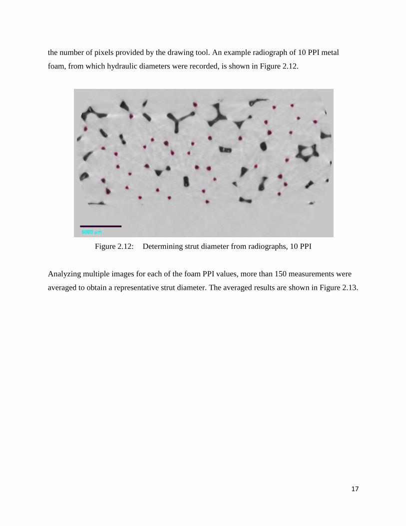
the number of pixels provided by the drawing tool. An example radiograph of 10 PPI metal

foam, from which hydraulic diameters were recorded, is shown in Figure 2.12.

Figure 2.12: Determining strut diameter from radiographs, 10 PPI

Analyzing multiple images for each of the foam PPI values, more than 150 measurements were

averaged to obtain a representative strut diameter. The averaged results are shown in Figure 2.13.

18

0.4

0.45

0.5

0.55

0.6

0.65

0 5 10 15 20 25

Ave

rag

e S

tru

t D

iam

ete

r [m

m]

Foam PPI

Figure 2.13: Strut diameter determined from X-ray μCT vs. foam PPI

The figure shows a negative correlation of strut diameter with foam PPI. The manufacturer

provided the ligament diameter information shown in Figure 2.14, with the arrows marking the

densities of the foam samples discussed here.

19

Figure 2.14: MFG Data Diameter

Table 2.2 shows how the average diameters obtained from the radiography analysis compare to

the diameter values provided by the manufacturer.

Foam

PPI

X-ray Data

[mm]

Mfg Data

[mm]

5 0.6023 -----

10 0.4641 0.3937

20 0.4169 0.2134

Table 2.2: Average strut diameters determined from X-ray μCT data compared to data

provided by the manufacturer

Disregarding the 5 PPI foam, as the manufacturer provided no corresponding data for the

diameter, it is clear that there is a significant difference between the manufacturer-reported

diameter and measured diameter. For these samples, the measured diameter was taken as the

more accurate value, as it was experimentally obtained rather than taken from a generalized

curve.

20

After analyzing the raw X-ray images for strut density, diameter, and cross-sectional geometry,

advanced image analysis software was required in order to extract additional geometric

information. As mentioned, commercially available software packages, like Amira®, are

commonly used for CT analysis. However, due to the structure of the metal foams, the pre-

packaged software was insufficient for the required analysis. Amira® could be used for

manipulating the images to create visual aids, but the software had difficulty differentiating the

pores. In the literature, at least two names of software specializing in foam image analysis were

mentioned. Ozella3D was considered intellectual property and unavailable to the public [63].

FoamView©, however, was provided as supplementary material online with the citing article

[61].

FoamView© requires the input of a series of X-ray CT images. After uploading these images, an

appropriate scale, and defining if the foam is black or white in the images, the software creates a

3D rendering. This initial rendering is a volume file, which requires a large amount of computing

power. A sample volume rendering is shown in Figure 2.15 for 10 PPI metal foam, where a fog

effect has been applied to show depth.

Figure 2.15: Foamview volume rendering, 10 PPI

21

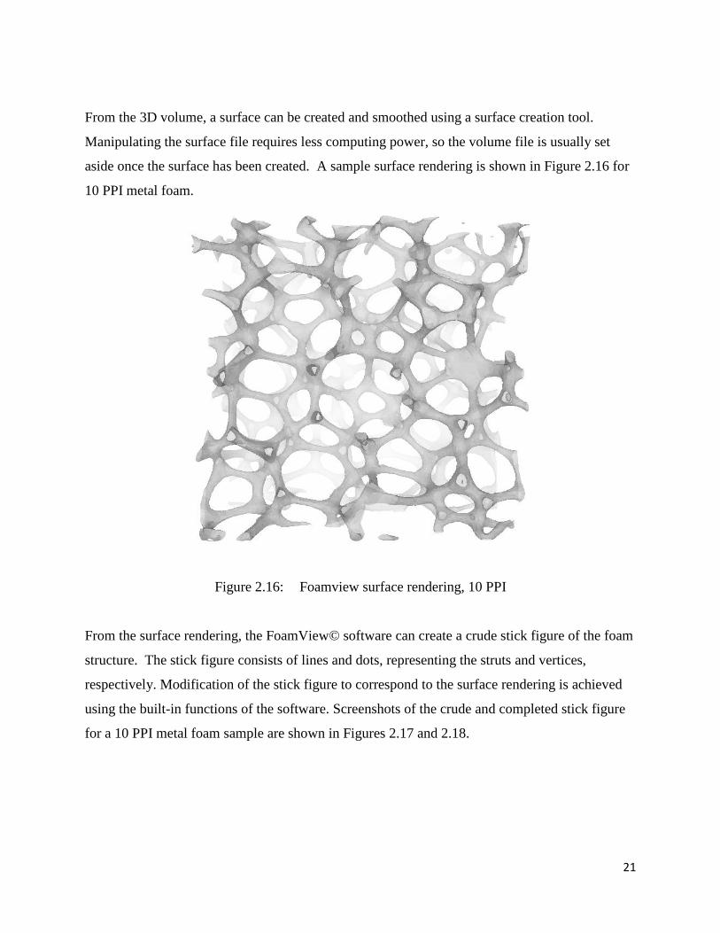
From the 3D volume, a surface can be created and smoothed using a surface creation tool.

Manipulating the surface file requires less computing power, so the volume file is usually set

aside once the surface has been created. A sample surface rendering is shown in Figure 2.16 for

10 PPI metal foam.

Figure 2.16: Foamview surface rendering, 10 PPI

From the surface rendering, the FoamView© software can create a crude stick figure of the foam

structure. The stick figure consists of lines and dots, representing the struts and vertices,

respectively. Modification of the stick figure to correspond to the surface rendering is achieved

using the built-in functions of the software. Screenshots of the crude and completed stick figure

for a 10 PPI metal foam sample are shown in Figures 2.17 and 2.18.

22

Figure 2.17: Foamview-generated crude stick figure, 10 PPI

Figure 2.18: Foamview completed stick figure, 10 PPI

23

The completed stick figure can be viewed alone for quicker response time and a simplified view

of the foam structure. During stick figure modification the software recognizes when windows

are formed and pores and completed. Windows are automatically shaded green, and blue spheres

appear to signify enclosed pores. FoamView© keeps a running total of the number of struts,

vertices, windows, and pores recognized in the stick figure. A screenshot of a completed stick

figure for 10 PPI metal foam and the FoamView© interface are shown in Figure 2.19, and for 5

PPI metal foam in Figure 2.20.

Figure 2.19: Foamview interface showing completed stick figure, 10ppi

24

Figure 2.20: Foamview interface showing completed stick figure, 5ppi

FoamView generates a report of measurements and statitistics from the completed stick figure.

The report includes information about the average strut length and orientation, window shapes,

pore (cell) sizes, and interior angles. Additional information such as surface area and volume can

be obtained from the surface and volume renderings; however, these values have not been

verified. The data can be exported as a Microsoft Excel Worksheet, or viewed in FoamView© as

histograms and tabulated values. FoamView reports for 20 PPI metal foam are shown in Figures

2.21 and 2.22.

25

(a)

(b)

(c)

Figure 2.21: Foamview histograms, 20 PPI: (a) strut length, (b) window area, (c) interior angle

26

Figure 2.22: Foamview report window, 20 PPI

The analysis was conducted for four metal foam samples. Two samples of 20 PPI metal foam

were chosen to investigate the repeatability between samples. Some variation was expected

considering that the two samples did not have identical void fractions. Two data sets were

analyzed with FoamView© for a 5 PPI sample to investigate the repeatability within a single

piece of foam. The results showed good repeatability between samples for 20 PPI foams and

datasets for the 5 PPI foam sample. The results for strut length and orientation of 5, 10, and 20

PPI metal foams, where the 5 PPI and 20 PPI data are averaged values from the two stick figures,

are summarized in Table 2.3.

27

Table 2.3: Summary of strut geometry from X-ray μCT data

Foam average orientation vectors azimuthal angle length standard

deviation

PPI x y z [°] [m] [m]

5 0.6830 0.5075 0.5250 58.3267 0.00192 0.35796

10 0.5540 0.5140 0.6550 49.0838 0.00149 0.34606

20 0.5325 0.6425 0.5515 56.5411 0.00112 0.37664

It is clear from the values shown in the table that there is considerable variation in the strut

length, which leads to a large standard deviation. This variation may be related to the foam

manufacturing process. If the metal foam is created from a gasified liquid metal, then the

structure does not reach equilibrium before solidification [61]. The strut length distributions for

the different foam samples are shown in Figure 2.23.

Figure 2.23: Strut length distribution

0

10

20

30

40

50

60

70

0 1 2 3 4

Freq

uen

cy

Strut Length [mm]

20 PPI B

20 PPI A

10 PPI

5 PPI

28

The data reflect variation in strut lengths for a given sample of foam and that the average strut

length becomes gradually larger as PPI decreases, which can be expected. If compared to the

strut length distribution in an ideal unit cell, the results would differ significantly. The Kelvin

unit cell has only one strut length, as all windows consist of regular polygons. The Weaire-

Phelan unit cell is comprised of four different strut lengths, which is still far from the actual foam

geometry, but it is a better representation of the metal foam than is the Kelvin unit cell.

The window shape distributions for the different foam samples are given in Figure 2.24 and are

compared to unit-cell models in Table 2.24. The predominance of pentagons supports the

adoption of the Weaire-Phelan unit cell; however, the presence of quadrilaterals suggests that

there may be room for improvement. Although the Kelvin unit cell does contain quadrilaterals, it

omits pentagons, which are the most frequently occurring shape in real foams. Thus, the choice

of the Weaire-Phelan unit cell is further supported.

Figure 2.24: Window shape distribution

29

Table 2.4: Window shape distribution (as a percentage of total) from X-ray μCT data compared

to ideal unit cells

FOAM

SAMPLE Triangles Quadrilaterals Pentagons Hexagons Heptagons+

5 PPI A 0.0 15.1 61.1 22.2 1.6

5 PPI B 0.0 15.1 61.1 22.2 1.6

10 PPI 0.4 12.6 69.1 17.9 0.0

20 PPI A 0.0 20.4 56.5 21.6 1.5

20 PPI B 0.4 15.6 65.9 17.7 0.4

Kelvin 0.0 42.9 0.0 57.1 0.0

Weaire-Phelan 0.0 0.0 88.7 11.3 0.0

2.6 Discussion and Conclusions

The X-ray μCT imaging was an effective and convenient means for obtaining a digitized

rendering of the real metal foam structures. Several conclusions were drawn from the X-ray

images, while specialized image analysis software allowed for the extraction of other geometric

data and characterization of the actual foam structure. Four aluminum foam samples were

analyzed: one 5 PPI sample, one 10 PPI sample, and two 20 PPI samples. The two 20 PPI

samples were chosen to investigate geometric differences between two samples of the same foam

PPI, from the same manufacturer.

The image analysis revealed a large variation in strut size, which highlighted the irregularity of

the metal foam structure. Standard deviations for the strut length were on the order of 40% of the

average value. Values for interior strut angles and average number of windows on a given pore

matched those provided in the literature as mathematical requirements. The distributions of the

window shapes were compared to the ideal unit cells as a means of determining the most

accurate model. The Weaire-Phelan unit cell was proven to be more accurate due to the dominate

30

presences of pentagonal windows, which are not included in the Kelvin unit cell. However, the

presence of quadrilateral windows suggests that improvements on the Weaire-Phelan unit cell

may exist, with respect to modeling metal foams.

In conclusion, the real structure of open-celled metal foams is highly irregular. This irregularity

can be attributed to the production process and is an inherent characteristic. In attempts to model

the behavior and characteristics of metal foams, many researchers assume an idealized geometry.

Current and future models could be improved by recognizing that the cross-sectional area of the

struts is triangular, rather than circular. Improvements can also be made by replacing the ideal

Kelvin unit cell model with the more complicated Weaire-Phelan unit cell. While the Weaire-

Phelan unit cell is currently more accurate in describing actual metal foams, there is still room

for improvement. As new unit cells are proposed, the Weaire-Phelan model may be replaced

with an ideal geometry that more closely matches the actual geometry of metal foams.

31

Chapter 3: Liquid Retention Behavior of Open-Cell Metal Foams

3.1 Background and Literature Review

A common concern in(air-side heat exchanger design is condensate removal. Condensate

retention can have a variety of detrimental effects on heat exchanger performance. The

accumulation of water droplets degrades heat exchanger performance by adding a thermal

resistance and blocking airflow, which increases pressure drop. There have been numerous

studies on evaluating retention behavior and enhancing condensate removal [27-33].

Open-celled metal foams have shown promise as a novel material for heat exchangers [10-17].

Researchers have recently provided data showing the high heat transfer enhancements that can

be achieved with the use of metal foam in place of louver fins [70]. However, information

regarding the water retention of metal foams is scanty.

In order to characterize the metal foam water retention characteristics, Al-6101-T6 samples were

evaluated using a basic testing method. With ongoing research being conducted to determine the

optimum heat exchanger configuration, to-scale heat exchanger unit samples were not tested.

The metal foam samples provide general results that can be considered representative,

independent of final heat exchanger configuration, when dealing with open-celled metal foams.

Small samples of AL-6106T, open-celled, metal foams were obtained with porosities of 5, 10,

20, and 40 pores per inch (PPI). Two samples are shown in Figure 3.1.

32

Figure 3.1: Open-cell aluminum metal foams of varying foam PPI

Two samples of each foam PPI were subjected to some basic dip tests in which the water

retention for quiescent, gravity-drained conditions was measured. Half of the samples were

treated with a Beomite process to examine the effects of surface treatment. The Beomite

treatment process consisted of submerging the metal foam samples in boiling, soapy water.

3.2 Experimental Methods

Some basic experiments were conducted to measure the water retention of several metal foam

samples. The experiment was designed to mimic gravity-induced drainage behavior of

completely wetted metal foam. By characterizing the foam individually and separately from a

particular heat exchanger design, it is expected that the results will be more general, with

applicability to current and future configurations.

A metal foam sample was fully submerged in a beaker of water. The metal foam sample was

then agitated to ensure full permeation and the release of trapped air bubbles. Once agitation was

complete, the metal foam sample was vertically lifted from the beaker, allowing gravity induced

drainage to begin. The water drainage was monitored until steady state was detected. The

sample was assumed to be at steady state when the water stopped dripping from the bottom.

33

The majority of the retained water formed a column at the bottom of the metal foam sample, with

some water being retained in single pores in a scattered/random manner, as shown in Figure 3.2.

The height of the water column, h, was measured using a scale before the metal foam sample and

retained water mass were measured using a balance with decigram accuracy. The sample was

then dried using compressed air before beginning the process again. Thirty measurements were

recorded for each sample.

Figure 3.2: Diagram of water retention behavior

In order to determine the effects of extraction speed, the tests were repeated at three different

rates of withdrawal. The sample was vertically removed from the water at fast, moderate, and

slow speeds. “Fast” withdrawals took approximately one second, “moderate” rates of withdrawal

required approximately 4 seconds, and “slow” withdrawals occurred over a period of 6-7

seconds. The sample was also tested at various orientations to evaluate anisotropy effects. Each

face was held parallel to the liquid-vapor interface during extraction, but orientation effects

proved to be negligible.

After plotting the data, it appeared that there was a change in trend for the water retention in the

10 PPI sample. Upon investigation, it was discovered that the capillary length of water is nearly

34

equivalent to the characteristic length of 10 PPI metal foam. The experiments were repeated for

ethylene glycol and 91% isopropyl alcohol (IPA) to investigate the effects of capillary length.

3.3 Experimental Results

Each dip test was repeated thirty times to obtain averaged results. The experiments were limited

to the four porosities available: 5, 10, 20, and 40 PPI; however, it is expected that the trends are

representative for a wider range of porosities. The experimental results for the untreated metal

foam samples were compared to the results for treated samples of the same foam PPI. The

treated samples we subjected to a Beomite process in which they were submerged in boiling

soapy water for five minutes. Dawn® dish soap was used. The surface Beomite process was

expected to decrease water retention by increasing the hydrophilic behavior of the metal foams.

The manufacturer provided a measurement of pores per inch (PPI) to characterize the metal foam

samples. An additional means of characterizing the metal foams is void fraction, or foam density.

The void fraction, , can be calculated using equation 3.1,

1 1f f

tot f tot

m V

V V

(3.1)

where fm ,

fV , and f are the mass, volume and density of the metal foam, respectively, and

totV is the total volume occupied by the foam sample when viewed as a solid rectangular prism.

A comparison of the foam PPI to the void fraction is shown in Figure 3.3.

35

0.9

0.92

0.94

0.96

0.98

1

0 10 20 30 40 50

Treated

Untreated

Vo

id F

ractio

n

Foam PPI

Figure 3.3: Void fraction vs. foam PPI

It is clear that there is no distinct correlation between foam PPI and void fraction. This suggests

that the foam PPI, alone, is an insufficient means for truly characterizing metal foams. For this

reason, both foam PPI and void fraction will be reported in the results.

In order to evaluate the sensitivity of liquid retention with respect to the rate of withdrawal, the

dip tests were conducted for three different extraction speeds. The slow, moderate, and fast rates

of withdrawal were somewhat arbitrary in that they are relative, occurring over time intervals of

approximately seven, four, and one second, respectively. . The results for total mass of water

retained in untreated and treated foams at various extraction speeds are shown in Figure 3.4 and

Figure 3.5, respectively.

36

0

2

4

6

8

10

12

0 10 20 30 40 50

fast

moderate

slow

To

tal M

ass o

f W

ate

r R

eta

ine

d [

g]

Foam PPI

Figure 3.4: Total water retained in untreated samples vs. foam PPI

37

0

2

4

6

8

10

12

0 10 20 30 40 50

fast

moderate

slow

Tota

l M

ass o

f W

ate

r R

eta

ined

[g]

Foam PPI

Figure 3.5: Total water retained in treated samples vs. foam PPI

The data presented in these figures suggest that the surface treatment has no significant effect on

the water retention in metal foam samples that have been subjected to gravity-induced drainage.

It can also be concluded from the data that water retention increases with foam PPI. In other

words, metal foams with smaller pore volumes retain more water than those with larger pore

sizes.

It was previously shown that foam PPI, in itself, is insufficient for characterizing the metal foam

samples. In order to highlight this point, the same data from Figures 3.4 and 3.5 have been re-

plotted with respect to void fraction in Figures 3.6 and 3.7.

38

0

2

4

6

8

10

12

0.9 0.92 0.94 0.96 0.98 1

fast

moderate

slow

Tota

l M

ass o

f W

ate

r R

eta

ine

d [

g]

Void Fraction

Figure 3.6: Total water retained in untreated samples vs. void fraction

39

0

2

4

6

8

10

12

0.9 0.92 0.94 0.96 0.98 1

fast

moderate

slow

To

tal M

ass o

f W

ate

r R

eta

ine

d [

g]

Void Fraction

Figure 3.7: Total water retained in treated samples vs. void fraction

When the data are plotted against void fraction, no overall trends seem to prevail. The results

would be more compelling if the treated and untreated foam samples had the same void fraction.

However, the manufacturer only provides the foam PPI as an exact value and reports the void

fraction as a range of 91-95% for these samples. The void fraction is difficult to control during

the manufacturing process, making the foam PPI the best means of classifying the metal foams,

albeit incomplete.

The water retention could be divided into two specific regions. Some of the water was retained in

a saturated column, while the rest was retained in the “unsaturated” region. In the saturated

region, the surface of the liquid-vapor interface was irregular, as the water filled complete pores

40

and followed the structure of the metal foam. The height of the saturated region was measured

based on an average height of the undulations/ripples of the surface at the liquid-vapor interface.

In the unsaturated region, the water was retained in scattered locations, filling individual pores.

The water retention behavior can be seen in Figure 3.8, where the two retention regions can be

seen in the images. Food coloring has been added to the water for better visualization. In

addition to the saturated and unsaturated retention regions, these images show that metal foam

samples with a higher PPI retains more water.

Figure 3.8: Water retention regions

Unsaturated region

Saturated region

5 PPI 20 PPI

41

The amount of water retained in the two regions could be determined from the measurement of

the saturated region height, h. Knowing the void fraction and volume of foam in the saturated

region, the amount of water in the column, mcalc, could be calculated from equation 3.2,

calc c liqm A h (3.2)

where Ac is the cross sectional area of the metal foam sample, and ρliq is the density of the liquid.

The mass of water in the unsaturated region could then be evaluated by applying conservation of

mass to the liquid, as given in equation 3.3,

liq wet fm m m (3.3)

where the mass of the liquid, mliq is determined from the difference in the mass of the wet foam,

mwet, and the mass of the dry foam sample, mf.

Comparing these values to the total mass of water retained, following equation 3.4, revealed that

approximately 50% of the total water retained was held in each region.

% 100%calc

iq

msaturated region

m

(3.4)

The percentage of water retained in the unsaturated region is plotted as a function of foam PPI in

Figure 3.9.

42

0

10

20

30

40

50

60

70

0 10 20 30 40 50

Treated

UntreatedPe

rce

nt

Ma

ss R

eta

ine

d in

Sa

tura

ted

Reg

ion

[%

]

Foam PPI

Figure 3.9: Percentage of the mass of water retained in the saturated region vs. foam PPI

The results for the treated and untreated foams shown an average of about 55% of the total water

retained being held in the unsaturated region. With these results and a model for the predicted

amount of water retained in the saturated region, the total mass of water retained can be

estimated.

The unsaturated region was also analyzed to determine the percentage of the volume occupied by

water. The results for treated and untreated metal foam samples are shown in Figures 3.10 and

3.11 with respect to foam PPI and extraction speed.

43

0

5

10

15

20

0 10 20 30 40 50

fast

moderate

slow

Pe

rce

nt

Vo

lum

e o

f W

ate

r [%

]

Foam PPI

Figure 3.10: Percentage of the volume occupied by liquid in the unsaturated region of

untreated samples vs. foam PPI

44

0

5

10

15

20

0 10 20 30 40 50

fast

moderate

slow

Pe

rcen

t V

olu

me

of

Wate

r [%

]

Foam PPI

Figure 3.11: Percentage of the volume occupied by liquid in the unsaturated region of treated

samples vs. foam PPI

A general trend of increasing volume percentage with increasing foam PPI is shown in these

plots. The same data are then re-plotted versus void fraction, as shown in Figures 3.12 and 3.13.

45

0

5

10

15

20

0.9 0.92 0.94 0.96 0.98 1

slow

moderate

fast

Pe

rce

nt

Vo

lum

e o

f W

ate

r [%

]

Void Fraction

Figure 3.12: Percentage of the volume occupied by liquid in the unsaturated region of

untreated samples vs. void fraction

46

0

5

10

15

20

0.9 0.92 0.94 0.96 0.98 1

fast

moderate

slow

Pe

rce

nt

Vo

lum

e o

f W

ate

r [%

]

Void Fraction

Figure 3.13: Percentage of the volume occupied by liquid in the unsaturated region of treated

samples vs. void fraction

Again it is apparent that foam density matters. Although the foam PPI paints an incomplete

picture of the foam, it is the preferred means of classification. The percent volume of water

retained in the unsaturated region tends to increase as foam PPI increases for both treated and

untreated foams. No such statement can be made regarding the void fraction. Although the data

show that about half of the total water retained is held in the unsaturated region, it occupies less

than 20% of the foam volume. This water is randomly distributed in single pores or small groups

of pores throughout the unsaturated region.

47

The data from the water retention dip tests show a change in trend between 5-10 PPI. Intuition

suggests that metal foams of 5 PPI will hold less water than samples of 10 PPI; however, the data

suggest otherwise, but the difference was small. Possible sources for this disagreement were

explored. The capillary length of water was discovered to be very close to a characteristic length

of metal foam with 10 PPI. The capillary length, λc, is defined by equation 3.5,

liq

c

liq g

(3.5)

where liq is the liquid-vapor surface tension, and g is the acceleration due to gravity.

In order to establish the effect of capillary length on the retention characteristics of metal foams,

additional dip tests were conducted with different fluids having capillary lengths different from

that of water, but near characteristic lengths of the foam samples. The liquid capillary lengths

and foam characteristic lengths are listed in Tables 3.1 and 3.2, respectively. Finding liquids

with satisfactory thermophysical properties, and compatibility with aluminum, was difficult.

Ethylene glycol and 91% isopropyl alcohol (rubbing alcohol) were chosen as two additional

liquids for the experiments.

Table 3.1: Capillary lengths for three fluids

Fluid Capillary Length

Water (H2O) 0.271 cm

Ethylene Glycol (EG) 0.209 cm

91% Isopropyl Alcohol (IPA) 0.184 cm

Table 3.2: Characteristic lengths of metal foam samples

5 PPI 10 PPI 20 PPI 40 PPI

Characteristic

Length (1/PPI)

0.508 cm 0.254 cm 0.127 cm 0.064 cm

Average Length

(X-ray CT data)

0.192 cm .0149 cm 0.112 cm ----

48

As the water retention results suggested, little dependence on surface treatment and extraction

speed, the number of dip tests for the two additional fluids was found. The data represent an

average value from thirty dip tests, all conducted at a moderate extraction speed. The total mass

of liquid retained is shown in Figures 3.14 and 3.15 with respect to foam PPI.

0

2

4

6

8

10

0 10 20 30 40 50

To

tal M

ass o

f Liq

uid

Re

tain

ed

[g]

Foam PPI

Figure 3.14: Mass of ethylene glycol retained vs. foam PPI

49

0

2

4

6

8

10

0 10 20 30 40 50

To

tal M

ass o

f Liq

uid

Re

tain

ed

[g]

Foam PPI

Figure 3.15: Mass of 91% isopropyl alcohol retained vs. foam PPI

These results show a positive correlation between liquid retention and foam PPI, as expected.

Analysis of the data showed similar results to the water dip test. Approximately 50% of the

liquid was contained in each of the retention regions, as shown in Figure3.16.

50

0

10

20

30

40

50

60

70

0 10 20 30 40 50

H2O (T)

H2O

EG (T)

EG

IPA

IPA (T)

Pe

rcen

t M

ass R

eta

ined

in

Sa

tura

ted

Regio

n [

%]

Foam PPI

Figure 3.16: Summary of percent mass of liquid retained in the saturated region

As with the water dip tests, the liquid retention in the unsaturated region was examined for the

ethylene glycol and isopropyl alcohol. The results for the percent of volume occupied by the

liquid in the unsaturated region are summarized for all three fluids in Figure 3.17.

51

0

2

4

6

8

10

12

14

0 10 20 30 40 50

H2O

EG

IPA

Pe

rce

nt

Vo

lum

e o

f L

iqu

id in

Un

satu

rate

d R

eg

ion

[%

]

Foam PPI

Figure 3.17: Summary of percentage of total volume occupied by liquid in the unsaturated

region vs. foam PPI

Combining the results from the three fluids for both treated and untreated samples, a linear

relation was found for the percentage of the total foam volume in the unsaturated region

occupied by liquid, as described by equation 3.6.

1 2(% )liqvol C PPI C (3.6)

where C1 and C2 are constants determined by the fluid. Equations for the individual fluids

achieve an R2 value for goodness of fit as high as 0.95 for the 91% isopropyl alcohol data where

C1 = 0.12 and C2 = 2.6, and values as low as R2=0.74 where C1=0.2 and C2=3.0 for water.

52

The results for the total mass retained of each liquid are summarized in Figure 3.18. As intuition

may suggest, the amount of liquid retained increases with foam PPI, or decreasing pore size.

This trend held true for each liquid that was tested.

0

2

4

6

8

10

0 10 20 30 40 50

H2O

EG

IPA

Liq

uid

Ma

ss R

eta

ined

[g

]

Foam PPI

Figure 3.18: Summary of total mass of liquid retained vs. foam PPI

3.4 Discussion and Conclusions

In characterizing the water retention behavior of metal foams, a series of dip tests were

conducted in which several parameters were varied. The manufacturer provided samples

53

classified by the foam PPI. This measurement, however, was determined to be insufficient in

truly characterizing the foam. Due to the manufacturing process, the void fraction is difficult to

control with great precision, so samples of the same foam PPI had different void fractions. If

samples of the same PPI also had the same void fraction, comparisons could be improved;

nevertheless, the data show a stronger dependence on foam PPI, and it is the method of

classification most commonly used in the literature

The data show no significant differences in the retention behavior of untreated surfaces and

surfaces treated with a Beomite process. The amount of liquid retained increased slightly with

extraction speed, as did the percentage of the total foam volume occupied by liquid in the

unsaturated region. The percentage of the volume occupied by liquid in the unsaturated region

increased linearly with foam PPI. It was also determined that about half of the total liquid

retained was held in the unsaturated region.

The results of these dip tests provide a basic description of the retention behavior of metal foams.

Researchers in the thermal sciences may be particularly interested in this information, because

there has been recent interest in the condensate retention of heat exchangers [27-33]. In Chapter

4, a model incorporating these results will be presented to describe the liquid retention behavior

in the saturated region.

54

Chapter 4: Modeling of Liquid Retention in Open-Cell Metal Foams

4.1 Model Formulation

The retention model is based on the assumption that surface tension is the sole force acting to

retain the liquid within the foam. Because the metal foam structure is highly irregular and

difficult to model geometrically, a uniform mesh was created to validate the model. A model of

the meshed volume was created using ProEngineer. Employing the services of the UIUC

MechSE Ford Lab, a rapid prototype of the regular 3D mesh was created from polyamide

powder using the Formiga P 100 Selective Laser Sintering System. The key concern was to

create the rapid prototypes using material that is insoluble in water so that dip tests could be

conducted. A photo of one sample is shown in Figure 4.1. Two meshes of different dimensions,

describe in Table 4.1, were created in order to verify the underlying physics of the model.

Figure 4.1: Image of regular mesh rapid prototype

55

Table 4.1: Regular mesh rapid prototype dimensions

Dimension Rapid Prototype A Rapid Prototype B

Overall 13.7 x 49.8 x 76.4 mm 13.6 x 50 x 76 mm

Side length of pore 1.5 mm 2.0 mm

Thickness of strut 0.4 mm 0.6 mm

The model was formulated by accounting for surface tension along two lines of contact for each

strut at the liquid-vapor interface, as seen from a plan-view. The total contact length, Lcontact,

could then be calculated for both rapid prototypes at various orientations from equation 4.1,

2contactL L (4.1)

where L is the total length of struts contributing to surface tension.

Following equation 4.2, the maximum weight of water, Wmax, that the sample could theoretically

hold was calculated.

max liq contactW L (4.2)

From the maximum weight and the density of the liquid, the height of the liquid column could be

calculated and converted to a number of pores. By conducting dip tests, the predicted height was

compared to the height of the liquid column found in experiments. Three different orientations

were used during the dip tests in order to validate the model. Both water and 91% isopropyl

alcohol were employed to support the generality of the model. The experimental results agreed

well with the predictions, with a retained weight usually less than 7% of the maximum weight.

The model validation results for both prototypes, with water as the fluid, are shown in Table 4.2.

56

Table 4.2: Results of prototype dip tests - model validation

4.2 Model Applied to Real Geometry from X-ray CT Data

Having verified the physics of the model, it was then applied to the foam, using geometric data

obtained from the X-ray CT analysis. Using average values for strut length, orientation, and

distribution, an average contact length, Lavg, can be calculated using equation 4.3, where lavg is

the average strut length. It is assumed that there will be two lines of contact for each strut in the

cross sectional area of the metal foam sample.

#

2

avg avg cXrayXray

strutsL l A

unit area

(4.3)

The average contact length, Lave, can then be compared to the required contact length, Lreq,

obtained from the dip test results. The required contact length can be calculated using equation

57

4.4, where dividing the weight of the liquid retained, Wliq, by the surface tension results in a

contact length required to hold the measured amount of water held in the foam.

liq

req

liq

WL

(4.4)

The results of the comparison are shown in Figures 4.2-4.4. The plots show the results for three

different liquids: water, isopropyl alcohol, and ethylene glycol.

0

0.1

0.2

0.3

0.4

0.5

0.6

0 5 10 15 20 25

Con

tact

Le

ng

th [

m]

Foam PPI

Figure 4.2: Model predictions for water using X-ray μCT geometry data

(Legend: Ltot and Lreq)

58

0

0.1

0.2

0.3

0.4

0.5

0.6

0.7

0.8

0 5 10 15 20 25

Con

tact

Len

gth

[m

]

Foam PPI

Figure 4.3: Model predictions for 91% IPA using X-ray μCT geometry data

(Legend: Ltot and Lreq)

59

0

0.2

0.4

0.6

0.8

1

1.2

0 5 10 15 20 25

Con

tact

Le

ng

th [

m]

Foam PPI

Figure 4.4: Model predictions for ethylene glycol using X-ray μCT geometry data

(Legend: Ltot and Lreq)

The results agree within the experimental uncertainty, which was determined statistically using

twice the standard deviation. The large variation of strut length inherent to the metal foam

structure leads to a greater uncertainty in the average contact length. This uncertainty is not

really an experimental uncertainty and can only be decreased by changing the structure of the

metal foam. Overall, the model provides good predictions when applying the average geometry

measurements obtained from the X-ray CT data.

60

4.3 Model Applied to Ideal Geometry from Weaire-Phelan Unit Cell

Applying the WP ideal unit cell geometry to the model can help determine if the ideal unit cell

describes the actual geometry well. The model has been verified by the rapid prototype dip tests

and supported by the comparison to metal foam dip test data. The major differences between the

predicted and experimental data can therefore be inferred to indicate discrepancies between the

idealized and actual geometry.

In order to determine the contact length of the Weaire-Phelan structure, a single unit cell was

considered. Contact lengths were calculated for two orientations of the unit cell by multiplying a

summation of the strut lengths, as seen from a plan-view, by two. The two orientations are

shown in Figure 4.5, with the struts contributing to contact length highlighted in red on Figure

4.5a.

Figure 4.5: WP unit cell - Struts contributing to surface tension (a) orientation #1,

(b) orientation #2

(a) (b)

61

The ideal unit cell was scaled to have an average strut length equal to that obtained from the X-

ray CT data. The probability of a unit cell holding water was then evaluated based on the average

strut length. The required contact length was calculated from equation 4.5 for surface tension

forces of a WP unit cell to retain a full cell of water.

wet avgWP WP

req WPliq WP

W lL

L (4.5)

The weight of the water, Wwet was determined under the assumption that each pore in the unit

cell would be full of water. This assumption was based on the dip test experiments in which the

water appeared to either fill pores completely or not at all. As the pores are equal in volume, a

single dodecahedron pore was chosen in order to simplify calculations. The volume of the single

pore was determined by dividing the polyhedron into twelve pentagonal pyramids that converged

at the center of the pore. The volume of a pentagonal pyramid, Vpent-pyramid, can be found using

equation 4.6.

pent pyramid ctc pentagonV d A (4.6)

where dctc is the center-to-center distance from the face of the pentagon windows to the center of

the pore, and Apentagon represents the area of one pentagonal window. This volume, when

multiplied by eight, yields the total volume of a single pore. The Weaire-Phelan unit cells

contains twelve pores of equal volume, thus the total volume of a unit cell is shown in equation

4.7.

3

8 12 0.5Xray

WP pentagon ctc

WP avg

lV A d

l

(4.7)

Assuming that the full volume of the unit cell was occupied by liquid, the weight of the liquid

could be calculated using equation 4.8.

62

max WP liqWPW V g

(4.8)

Performing a force balance on the unit cell related the weight of the liquid to the contact length

required for surface tension forces to support this weight. The force balance is shown in equation

4.9, where Li is the interfacial contact length.

max

Xray

liq iWP WPWP avg

lW L

l

(4.9)

The required contact length was then compared to the contact length as determined from the unit

cell geometry. The total contact lengths were converted to average strut lengths for easier

comparison. A Z-factor was used to relate the required strut length to a standardized normal

distribution of the measured strut length. The z-factor was calculated from equation 4.10, where

the average and standard deviation, Xray , values were taken from the X-ray CT data.

req avgWP Xray

WP

Xray

l lZ

(4.10)

Consulting a standard normal (Z) table, the probability of the strut length being less than or equal

to the required length could be determined. When the probability of the strut length being greater

than the required length was at least 50%, it was assumed that the unit cell would hold the liquid.

It was otherwise assumed that the unit cell would not retain any liquid.

Vertical stacking of unit cells was then simulated to determine the height of the liquid column

that would be retained. The translational distance of the unit cell could be used to convert the

number of unit cells being stacked to a measurement of height. The contact length remained the

same, as the same struts (seen from the plan-view) contributed to surface tension, but the volume

increased. Again it was assumed that the unit cells would hold water while the probability

remained 50% or greater. Both unit cell orientations were evaluated for stacking height. A plot of

the predicted and experimental values is shown in Figure 4.6, along with 30% error lines. Using

63

the statistical uncertainty of two standard deviations, every predicted point would agree well with

the experimental results. Having more confidence in the results, 30% error lines have been

plotted rather than adding statistics-based error bars. It is clear from the data that orientation #2

always is always predicted to hold less liquid retention than orientation #1. Although other

orientations may occur, only these two were considered. There was little variation in the total

contact lengths of the two orientations, so these data should represent the general ideal model

well.

0

0.5

1

1.5

2

2.5

3

3.5

4

0 0.5 1 1.5 2 2.5 3 3.5 4

WP 1

WP 2

Exp Data

-30%

+30%

Pre

dic

tio

n [

# u

nit c

ells

]

Experimental Results [# unit cells]

Figure 4.6: Model predictions for WP unit cell compared to dip test results

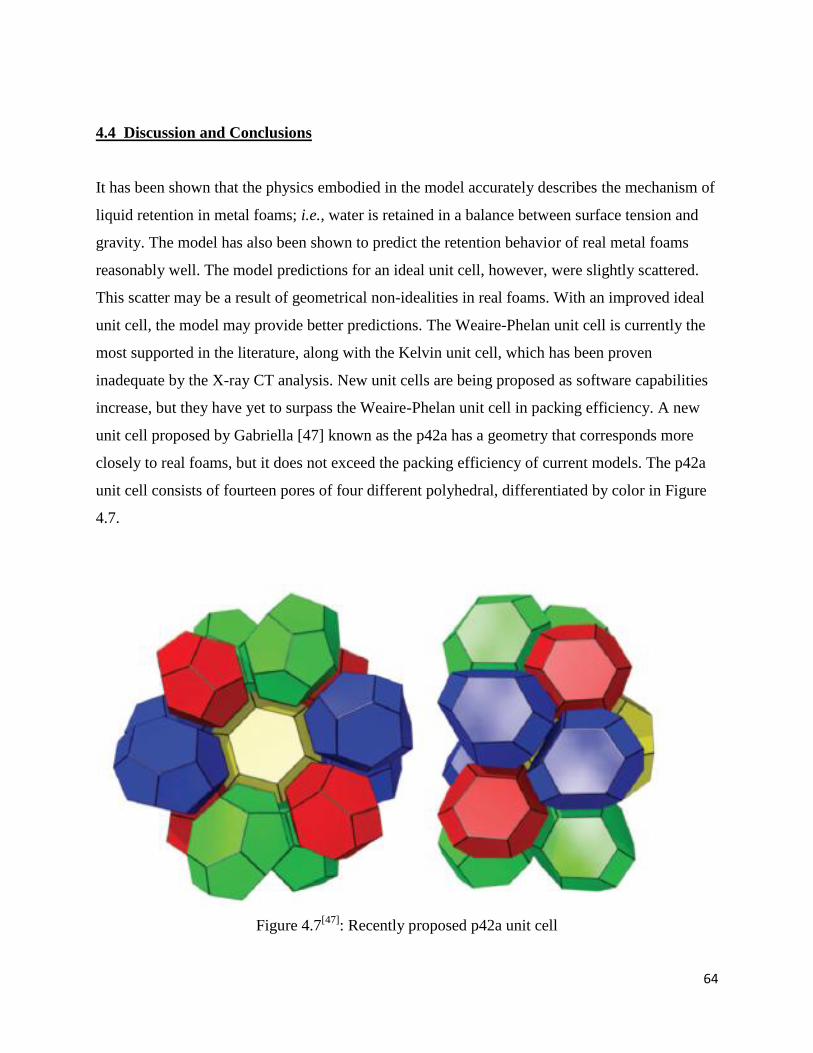
64

4.4 Discussion and Conclusions

It has been shown that the physics embodied in the model accurately describes the mechanism of

liquid retention in metal foams; i.e., water is retained in a balance between surface tension and

gravity. The model has also been shown to predict the retention behavior of real metal foams

reasonably well. The model predictions for an ideal unit cell, however, were slightly scattered.

This scatter may be a result of geometrical non-idealities in real foams. With an improved ideal

unit cell, the model may provide better predictions. The Weaire-Phelan unit cell is currently the

most supported in the literature, along with the Kelvin unit cell, which has been proven

inadequate by the X-ray CT analysis. New unit cells are being proposed as software capabilities

increase, but they have yet to surpass the Weaire-Phelan unit cell in packing efficiency. A new

unit cell proposed by Gabriella [47] known as the p42a has a geometry that corresponds more

closely to real foams, but it does not exceed the packing efficiency of current models. The p42a

unit cell consists of fourteen pores of four different polyhedral, differentiated by color in Figure

4.7.

Figure 4.7[47]

: Recently proposed p42a unit cell

65

66

Chapter 5: Summary

Open-cell metal foam is a promising material for heat exchangers. Many researchers have been

attempting to characterize metal foam and its thermal-hydraulic performance. However, the

geometric models adopted in the literature vary from source to source. In order to determine the

most applicable geometric model, the actual geometry of several metal foam samples was

characterized using X-ray μCT. The analysis revealed a large deviation in strut length, which

highlighted the randomness and irregularity of the foam structure. The average description of a

pore was determined, revealing a predominance of pentagonal windows as well as other features.

After examining several geometric models of foam structures, it was determined that the Weaire-

Phelan unit cell best described open-cell metal foam structures. Analytical models requiring

geometric descriptions of metal foam should follow this geometry rather than the Kelvin unit cell

or other simplified descriptions. The X-ray μCT data also revealed the triangular cross-sections

of the foam struts. Many of the current models describing the thermal-hydraulic performance of

metal foams assume struts with circular cross-sections. By adopting a triangular cross-section,

these and future models could be improved.

When considering metal foam as an air-side heat exchanger material, knowledge of the

condensate retention behavior is valuable. Some experiments were conducted under various

conditions in order to characterize the liquid retention behavior of open-cell metal foams. The

results were grouped into two distinct retention regions, where each region held approximately

half of the total liquid. The data showed an increase in liquid retention as foam PPI increased, as

intuition suggests. It was also determined that the amount of liquid retained increases linearly

with foam PPI in the unsaturated region.

A model based on surface tension was developed to predict the liquid retention in open-cell

metal foam. The model was applied to the real geometry, as determined by the X-ray μCT

analysis, and the WP ideal geometry. The model agreed well with the dip test data for both

geometries within the limits of uncertainty. These results may be useful in future heat exchanger

design, and similar analyses could be applied to a wider range of metal foams for more

generalized results.

67

References

1. Bastawros, A., & Evans, A. G. (1999). “Optimum performance of cellular metal heat sinks

for thermal management of high power electronics.” American Society of Mechanical

Engineers, EEP, 26(3), pp. 733-734.

2. Ohrndorf, A., Krupp, U., & Christ, H. -. (2006). “Metallic open-cell foams - A promising

approach to fabricating good medical implants.” Technology and Health Care, 14(4-5), pp.

201-208.

3. Fuganti, A., Lorenzi, L., Hanssen, A. G., & Langseth, M. (2000). “Aluminium foam for

automotive applications.” Advanced Engineering Materials, 2(4), pp. 200-204.

4. Nabavi, A., & Vahdati Khaki, J. (2010). A novel method for manufacturing of aluminum

foam sandwich panels. Surface and Interface Analysis, 42(4), 275-280.

5. Surace, R., De Filippis, L. A. C., Ludovico, A. D., & Boghetich, G. (2010). Application of

taguchi method for the multi-objective optimization of aluminium foam manufacturing

parameters. International Journal of Material Forming, 3(1), 1-5.

6. Carcel, B., Carcel, A. C., Perez, I., Fernandez, E., Barreda, A., Sampedro, J., et al. (2009).

Manufacture of metal foam layers by laser metal deposition. Paper presented at the , 7131

7. Barletta, M., Gisario, A., Guarino, S., & Rubino, G. (2009). Production of open cell

aluminum foams by using the dissolution and sintering process (DSP). Journal of

Manufacturing Science and Engineering, Transactions of the ASME, 131(4), 0410091-

04100910.

8. Fernández, P., Cruz, L. J., & Coleto, Y. J. (2009). Manufacturing processes of cellular

metals. part II. solid route, metals deposition, other processes. [Procesos de fabricación de

metales celulares. Parte ii: Vía sólida, deposición de metales, otros procesos] Revista De

Metalurgia (Madrid), 45(2), 124-142.

9. Fernández, P., Cruz, L. J., & Coleto, J. (2008). Manufacturing processes of cellular metals.

part I: Liquid route processes. [Procesos de fabricación de metales celulares. Parte I:

Procesos por vía líquida] Revista De Metalurgia (Madrid), 44(6), 540-555.

10. Han, X., Wang, Q., Park, Y., T'Joen, C., Sommers, A., & Jacobi, A. M. (2009). A review of

metal foam and metal matrix composites for heat exchangers and heat sinks. International

Journal of Refrigeration

68

11. Dai, Z., Nawaz, K., Park, Y., Chen, Q., & Jacobi, A. M. (2009). A comparison of metal-foam

heat exchangers to compact multi-louver designs for air-side heat transfer applications.

Proceedings of the Seventh International Conference on Enhanced, Compact and Ultra-

Compact Heat Exchangers: From Microscale Phenomena to Industrial Applications, San

Jose, Costa Rica, , 49-57

12. Boomsma, K., Poulikakos, D., & Zwick, F. (2003). “Metal foams as compact high

performance heat exchangers.” Mechanics of Materials, 35(12), pp. 1161-1176

13. Ghosh, I. (2009). “How good is open-cell metal foam as heat transfer surface?” Journal of

Heat Transfer, 131(10), pp. 1-8.

14. Zhang, G., Yang, L., & Sun, F. (2010). “Experimental investigation on pressure drop and

heat transfer characteristics in metal foam heat exchanger.” Wuhan Ligong Daxue Xuebao

(Jiaotong Kexue Yu Gongcheng Ban)/Journal of Wuhan University of Technology

(Transportation Science and Engineering), 34(5), pp. 986-989.

15. Elayiaraja, P., Harish, S., Wilson, L., Bensely, A., & Lal, D. M. (2010). “Experimental

investigation on pressure drop and heat transfer characteristics of copper metal foam heat

sink.” Experimental Heat Transfer, 23(3), pp. 185-195.

16. T'Joen, C., De Jaeger, P., Huisseune, H., Van Herzeele, S., Vorst, N., & De Paepe, M.

(2010). “Thermo-hydraulic study of a single row heat exchanger consisting of metal foam

covered round tubes.” International Journal of Heat and Mass Transfer, 53(15-16), pp.

3262-3274.

17. Zhao, C. Y., Lu, W., & Tassou, S. A. (2006). “Thermal analysis on metal-foam filled heat

exchangers. part II: Tube heat exchangers.” International Journal of Heat and Mass

Transfer, 49(15-16), pp. 2762-2770.

18. Dai, Z., Nawaz, K., Park, Y. G., Bock, J., & Jacobi, A. M. (2010). Correcting and extending

the boomsma-poulikakos effective thermal conductivity model for three-dimensional, fluid-

saturated metal foams. International Communications in Heat and Mass Transfer, 37(6),

575-580.

19. Calmidi, V. V., & Mahajan, R. L. (1999). Effective thermal conductivity of high porosity

fibrous metal foams. Journal of Heat Transfer, 121(2), 466-471.

69

20. Bhattacharya, A., Calmidi, V. V., & Mahajan, R. L. (2002). Thermophysical properties of

high porosity metal foams. International Journal of Heat and Mass Transfer, 45(5), 1017-

1031.

21. Mahjoob, S., & Vafai, K. (2008). “A synthesis of fluid and thermal transport models for

metal foam heat exchangers.” International Journal of Heat and Mass Transfer, 51(15-16),

pp. 3701-3711

22. Zhao, C. Y., Dai, L. N., Tang, G. H., Qu, Z. G., & Li, Z. Y. (2010). “Numerical study of

natural convection in porous media (metals) using lattice boltzmann method (LBM).”

International Journal of Heat and Fluid Flow, 31(5), pp. 925-934.

23. Ghosh, I. (2010). “Deterioration in heat transfer due to axial conduction of heat in open cell

metal foam.” Porous Media and its Applications in Science, Engineering, and Industry: 3rd

Interntational Conference, 1254 pp. 254-259.

24. Du, Y. P., Qu, Z. G., Zhao, C. Y., & Tao, W. Q. (2010). “Numerical study of conjugated heat

transfer in metal foam filled double-pipe.” International Journal of Heat and Mass Transfer,

53(21-22), pp. 4899-4907

25. Giani, L., Groppi, G., & Tronconi, E. (2005). “Heat transfer characterization of metallic

foams.” Industrial and Engineering Chemistry Research, 44(24), pp. 9078-9085.

26. Briano-Calcagno, C., Fontánez-Delgado, J., & Dukhan, N. (2004). “Characterization of the

heat transfer in open-cell metal foam” High Performance Structures and Materials II, pp.

243-252.

27. Sommers, A. D., & Jacobi, A. M. (2009). “Modeling the retention of water droplets on

topographically-modified, micro-grooved aluminum.” Proceedings of the 2008 ASME

Summer Heat Transfer Conference, 2 pp. 317-326.

28. Xu, X., Leung, C., Chan, M., & Deng, S. (2007). “Condensate retention on a louver-fin-and-

tube air cooling coil.” International Journal of Refrigeration, 30(3), pp. 409-417.

29. Zhong, Y., Joardar, A., Gu, Z., Park, Y., & Jacobi, A. M. (2005). “Dynamic dip testing as a

method to assess the condensate drainage behavior from the air-side surface of compact heat

exchangers.” Experimental Thermal and Fluid Science, 29(8), pp. 957-970.

30. Min, J., & Webb, R. L. (2001). “Condensate formation and drainage on typical fin

materials.” Experimental Thermal and Fluid Science, 25(3-4), pp. 101-111.

70

31. Yau, K. K., Cooper, J. R., & Rose, J. W. (1986). “HORIZONTAL PLAIN AND LOW-

FINNED CONDENSER TUBES - EFFECT OF FIN SPACING AND DRAINAGE STRIPS

ON HEAT TRANSFER AND CONDENSATE RETENTION.” Journal of Heat Transfer,

108(4), pp. 946-950.

32. Bryant, J. A., O'Neal, D. L., & Parker, B. (1995). “Study on the use of a hydrophobic coating

to enhance condensate drainage on a heat pump heat exchanger.” American Society of

Mechanical Engineers, Advanced Energy Systems Division AES, 34, pp. 89-98.

33. Liu, L., Jacobi, A. M., & Chvedov, D. (2009). “A surface embossing technique to create

micro-grooves on an aluminum fin stock for drainage enhancement.” Journal of

Micromechanics and Microengineering, 19(3).

34. Sir Thomson, W. (1887). “On the division of space with minimum partitional area.” Acta

Mathematica, 11(1-4), pp.121-134.

35. Rivier, N. (1996). “Seifenblasenrhetorik, or the Sound of the Last Trumpet?” Forma. 11(3),

pp.195-198.

36. Almgren, F., & Taylor, J. E. “Soap Bubble Clusters”

37. Weaire, D., & Phelan, R. (1994). “A counter-example to Kelvin's conjecture on minimal

surfaces.” Philosophical Magazine Letters, 69(2), pp. 107-10.

38. Weaire, D. & Phelan, R. (1994). “The structure of monodisperse foam.” Philosophical

Magazine Letters, 70(5), pp. 345-50.

39. Rivier, N., & Aste, T. (1996). “Organized Packing.” Forma, 11(3), pp. 223-231.

40. Kusner, R., & Sullivan, J. M. (1996). “Comparing the Weaire-Phelan Equal-Volume Foam to

Kelvin‟s Foam.” Forma, 11(3), pp. 233-242.

41. Aboav, D. A. (1996). “Kelvin‟s „Division of Space‟, and its Aftermath.” Forma, 11(3), pp.

243-254.

42. Kraynik, A. M., & Reinelt, D. A. (1996). “Elastic-Plastic Behaviour of a Kelvin Foam.”

Forma, 11(3), pp. 255-270.

43. Coxeter, H. S. M. (1958). “Close-Packing and Froth.” Illinois J. Math, 2(4B), pp. 746-758.

44. Phelan, R. (1996). “Generalisations of the Kelvin Problem and Other Minimal Problems.”

Forma, 11(3), pp. 287-302.

45. Honda, H., Morita, T., & Tanabe, A. (1979). Establishment of epidermal cell columns in

mammalian skin: Computer simulation. Journal of Theoretical Biology, 81(4), pp. 745-759.

71

46. Tanemura

47. Gabbrielli, R. (2009). A new counter-example to Kelvin's conjecture on minimal surfaces.

Philosophical Magazine Letters, 89(8), 483-491.

48. Sullivan, R. M., Ghosn, L. J., & Lerch, B. A. (2008). A general tetrakaidecahedron model for

open-celled foams. International Journal of Solids and Structures, 45(6), 1754-1765.

49. Ross, S., & Prest, H. F. (1986). On the morphology of bubble clusters and polyhedral foams.

Colloids and Surfaces, 21(C), 179-192.

50. Williams, R. E. (1968). Space-filling polyhedron: Its relation to aggregates of soap bubbles,

plant cells, and metal crystallites. Science, 161(3838), 276-277.

51. Saadatfar, M., Barry, J., Weaire, D., & Hutzler, S. (2008). “Ordered cylindrical foam

structures with internal bubbles.” Philosophical Magazine Letters, 88(9-10), pp. 661-668.

52. van der Net, A., Delaney, G. W., Drenckhan, W., Weaire, D., & Hutzler, S. (2007).

“Crystalline arrangements of microbubbles in monodisperse foams.” Colloids and Surfaces

A: Physicochemical and Engineering Aspects, 309(1-3), pp. 117-124.

53. Kriszt, B., & Faure, K. (2003). “Characterization of the cell structure of metallic foams.”

[Charakterisierung der zellstruktur von metallischen schäumen] Praktische

Metallographie/Practical Metallography, 40(11), pp. 537-555.

54. McDonald, S. A., Mummery, P. M., Johnson, G., & Withers, P. J. (2006). “Characterization

of the three-dimensional structure of a metallic foam during compressive deformation.”

Journal of Microscopy, 223(2), pp. 150-158.

55. Krishnan, S., Murthy, J. Y., & Garimella, S. V. (2006). “Direct Simulation of Transport in

Open-Cell Metal Foam.” Journal of Heat Transfer, 28(8), pp. 793-800.

56. J.A.F. Plateau (1873) “Statique Experimentale et Theorique des Liquides Soumis aux Seules

Forces Moleculaires,” Gauthier-Villard, Paris.

57. Matzke, E. B., (1946). “The Three-Dimensional Shape of Bubbles in Foam-An Analysis of

the Role of Surface Forces in Three-Dimensional Cell Shape Determination.”American

Journal of Botany, 33, pp. 58-80.

58. Brakke, K. A. (1992). “Minimal surfaces, corners, and wires”. The Journal of Geometric

Analysis, 2(1), 11-36.

59. www.steelpillow.com

72

60. Schmierer, E. N., Razani, A., Keating, S., & Melton, T. (2004). “Characterization of high

porosity open-celled metal foam using computed tomography.” American Society of

Mechanical Engineers, Heat Transfer Division, HTD, 375(2), pp. 415-424.

61. Montminy, M. D., Tannenbaum, A. R., & MacOsko, C. W. (2004). “The 3D structure of real

polymer foams.” Journal of Colloid and Interface Science, 280(1), pp. 202-211.

62. Saadatfar, M., Garcia-Moreno, F., Hutzler, S., Sheppard, A. P., Knackstedt, M. A., Banhart,

J., et al. (2009). “Imaging of metallic foams using X-ray micro-CT.” Colloids and Surfaces

A: Physicochemical and Engineering Aspects, 344(1-3), pp. 107-112.

63. Michaeli, W., Schrickte, L., Berdel, K., “Structural analysis of polymeric foams.”

Proceedings of the Skyscan User Meeting 2009. pp. 51-54.

64. Lin, C. L., Videla, A. R., Yu, Q., & Miller, J. D. (2010). “Characterization and analysis of

porous, brittle solid structures by X-ray micro computed tomography.” JOM, 62(12), pp. 86-

89.

65. Vabre, A., Legoupil, S., Buyens, F., Gal, O., Riva, R., Gerbaux, O., et al. (2007). “Metallic

foams characterization with X-ray microtomography using Medipix2 detector.” Nuclear

Instruments and Methods in Physics Research, Section A: Accelerators, Spectrometers,

Detectors and Associated Equipment, 576(1), pp. 169-172.

66. Maire, E., Fazekas, A., Salvo, L., Dendievel, R., Youssef, S., Cloetens, P., et al. (2003). “X-

ray tomography applied to the characterization of cellular materials. related finite element

modeling problems.” Composites Science and Technology, 63(16), pp. 2431-2443.

67. Winter Jr., J. M., Green Jr., R. E., Waters, A. M., & Green, W. H. (1999). “X-ray computed

tomography of ultralightweight metals.” Research in Nondestructive Evaluation, 11(4), pp.

199-211.

68. www.xviewct.com

69. www.xradia.com

70. Nawaz, K., Bock, J., Dai, Z. & Jacobi, A. (2010). “Experimental Studies to Evaluate the Use

of Metal Foams in Highly Compact Air-Cooling Heat Exchangers.” International

Refrigeration and Air Conditioning Conference at Purdue. Paper Number 2502.

71. www.Wikipedia.org

72. www.ndt.ed.org

73

73. Bodla, K.K., Murthy, J.Y., and Garimella, S.V. (2010). “Microtomography-Based Simulation

of Transport through Open-Cell Metal Foams.” Numerical Heat Transfer, Part A:

Applications. 58(7), pp. 527-544.

74. Kline, S.J. and F.A. McClintock. (1953). “Describing uncertainties in single-sample

experiments.” Mechanical Engineering. 75, pp. 3-8.

74

Appendix A: Experimental Results: Dip Test Raw Data—Water

MODERATE RATE OF WITHDRAWAL

5 PPI-Treated

5 PPI-Untreated Ac 0.734375 in2 Ac 0.765625 in2

Vtot 2.524414 in3 Vtot 2.727539 in3

mwet 9.1 g mwet 9.8 g

φ 0.920803

φ 0.921062

Table A.1: Raw data, 5 PPI , mwet [g] h [in*64]

mwet [g] h [in*64]

14.1 14

13.6 14 13.8 14

13.9 14

13.8 12

13.9 16 13.7 12

13.8 14

13.5 10

13.9 14 14 12

13.5 14

13.8 14

13.5 14 13.4 12

14 16

13.7 16

13.7 16 13.4 14

13.7 12

14.1 14

13.7 12 13.7 14

13.9 14

14 14

14.4 14 13.2 12

13.9 14

13.5 12

13.6 14 13.6 12

13.6 12

13.8 14

13.8 16 14.1 14

13.8 14

13.9 12

13.8 12 13.7 12

14.3 14

13.5 10

14.2 14 13.9 14

13.8 16

13.5 14

13.7 12 13.7 10

13.9 16

13.4 12

14.1 16 13.7 12

14.1 16

13.4 12

13.9 14 13.7 14

14.1 12

14 14

13.7 12 13.9 12

13.5 12

75

10 PPI-Treated

10 PPI-Untreated Ac 0.71875 in2 Ac 0.71875 in2

Vtot 2.515625 in3 Vtot 2.493164 in3

mwet 9.3 g mwet 8.1 g

0.918779

0.928622

Table A.2: Raw Data, 10 PPI mwet [g] h [in*64]

mwet [g] h [in*64] 13.1 12

12.4 14

12.8 12

11.9 12 13.1 14

11.6 12

13.2 14

12 12 13.1 12

11.9 12

13.5 14

12.3 12 12.8 12

12.2 12

13.1 12

11.8 12 13.2 14

12.1 14

13 12

12.5 12 13 12

11.9 12

13.2 12

12.1 12 13.2 12

11.8 12

13.1 12

11.9 14 12.9 12

11.9 12

13.1 12

12 12 13.2 14

11.8 10

13 12

12.5 14 13 12

12.5 14

13.1 14

12 12 12.9 12

11.9 12

13.4 14

12.1 14 13.1 12

12.1 12

12.7 10

11.9 12 13.3 12

12.3 14

13.4 12

12 14 13.1 12

12 14

12.9 12

12.5 12 13.4 14

12.4 14

13.1 12

12.4 14

76

20 PPI-Treated

20 PPI-Untreated Ac 0.703125 in2 Ac 0.688477 in2

Vtot 2.460938 in3 Vtot 2.409668 in3

mwet 5.8 g mwet 9.2 g

0.948221

0.91612

Table A.3 Raw Data, 20 PPI mwet [g] h [in*64]

mwet [g] h [in*64] 11.8 20

15.9 22

12.1 22

15.5 24 11.2 20

15.6 22

11.6 20

15.7 24 11.8 20

16 24

11.9 22

15.9 22 11.7 20

16 24

11.7 20

16.1 24 11.9 22

15.3 20

11.6 20

15.7 22 11.4 18

15.9 24

11.9 20

15.7 22 12 22

15.6 24

12 22

15.9 24 11.9 22

15.7 20

11.8 20

15.5 22 11.6 20

16.2 24

12.1 22

15.4 22 12.4 22

15.7 20

11.3 18

15.8 24 11.5 18

15.9 22

12 20

16 24 12 20

15.7 22

11.7 20

15.5 20 11.6 20

16 24

11.7 20

15.9 22 11.5 20

16.1 24

11.8 20

15.6 20 11.6 20

16.2 24

12.2 22

15.9 22 11.4 20

11.7 20

77

40 PPI-Treated

40 PPI-Untreated Ac 0.734375 in2 Ac 0.717773 in2

Vtot 2.570313 in3 Vtot 2.489777 in3

mwet 7.8 g mwet 9.5 g

0.933329

0.916171

Table A.4: Raw Data, 40 PPI mwet [g] h [in*64]

mwet [g] h [in*64]

15.3 20

17.7 28 15.8 18

17.5 26

15.5 18

17.4 28 15.6 16

17.8 28

16.3 22

17.3 26 16.5 22

17.8 30

16.3 18

17.3 28 17.3 24

17.2 28

17.2 20

17.3 28 17.4 26

17.6 30

17.9 24

17.2 28 17.8 26

17.4 28

18 26

17.4 28 17.4 24

17.1 28

17.8 26

17.2 30 17.6 24

17.4 30

18 24

17.4 28 17.8 26

17.6 30

17.8 26

17.1 28 17.9 24

16.9 28

17.9 24

17.6 28 17.6 26

17 26

17.7 22

17 26 17.6 22

17.8 30

17.5 24

17.4 30 17.7 24

17.7 28

17.5 26

17.8 28 17.8 24

17.7 30

17.7 26

17.4 28 17.7 24

17.7 28

78

FAST AND SLOW RATES OF WITHDRAWAL Table A.5: Raw Data, 5 PPI, fast and slow rates of withdrawal

5 PPI treated untreated fast slow fast slow mwet [g] h [in*64] mwet [g] h [in*64] mwet [g] h [in*64] mwet [g] h [in*64] 14.4 16 12.8 16 14.3 12 13.1 12 14.2 14 12.4 14 14.6 14 12.6 14 14.3 16 12.4 14 14.6 14 12.9 12 14.2 16 12.4 14 14.6 16 12.7 12 14.4 16 12.1 14 14.3 12 13 12 14.7 16 12.5 12 14.3 12 12.7 14 14.7 18 12.7 14 14.6 16 13 14 14.4 16 12.7 16 14.7 16 12.9 14 14.8 16 12.6 14 14.9 14 13 14 14.4 16 12.2 12 14.7 16 12.9 14 14.9 18 12.2 14 14.4 16 12.8 12 14.2 14 12.6 14 14.5 16 12.5 12 14.3 16 12.6 14 14.6 14 12.9 12 14.8 16 12.1 14 14.9 14 12.9 14 14.7 16 12.5 12 14.6 14 12.9 12 14.5 14 12.8 14 14.8 14 12.8 12 14.3 14 12.6 14 15 16 12.8 12 14.6 16 12.6 12 14.8 14 12.9 14 14.2 14 12.5 14 15 16 12.8 12 14.4 16 12.3 12 14.8 14 12.7 14 14.3 16 12.6 16 14.8 14 12.6 14 14.3 14 12.4 14 14.9 16 12.9 12 14.4 14 12.2 14 14.3 14 12.8 14 14 14 12 12 15.1 16 12.7 12 14.4 16 12.3 12 14.7 14 12.9 12 14.4 16 12.6 12 14.7 14 13 14 14.6 16 12.2 12 14.5 14 12.5 12 14.4 16 12.2 12 14.2 12 12.8 14 14.5 14 12.5 14 14.7 14 12.8 12 14.6 14 12.5 14 14.5 14 12.8 12

79

Table A.6: Raw Data, 10 PPI, fast and slow rates of withdrawal

10 PPI treated untreated fast slow fast slow mwet [g] h [in*64] mwet [g] h [in*64] mwet [g] h [in*64] mwet [g] h [in*64] 13.8 16 12 12 12.7 14 10.8 8 14 14 12.2 12 13.2 12 10.8 8 14.1 16 12.2 12 12.9 12 10.9 8 14.8 16 12.1 12 13 12 10.9 10 14.2 16 12.1 12 12.6 14 10.8 8 14.1 16 12.2 12 13.1 12 10.8 8 14.2 14 12.2 12 12.7 12 10.8 10 14.2 16 12.2 14 12.9 12 10.7 10 14.1 14 12.2 14 13 14 10.7 8 14 14 11.9 12 13.1 14 10.8 8 13.9 14 12.1 14 12.4 12 10.7 10 14.4 14 12 12 13.1 14 10.6 8 14.3 16 12 12 13.1 14 10.7 8 14.3 14 12.1 12 13 14 10.9 10 14.7 16 12.2 12 12.9 14 10.6 8 14 16 12.1 12 12.9 14 11.1 10 14.3 14 12.1 12 13.4 14 10.7 8 14.2 14 12.1 12 21.9 14 10.8 10 14.3 16 12.4 12 13.2 14 10.8 8 14.3 16 12 10 12.9 14 10.6 8 14.4 16 12 12 12.9 14 10.6 8 13.8 14 12.1 12 12.9 14 10.6 8 14.1 14 12 12 13 14 10.8 10 14.5 16 11.9 12 13 14 10.8 8 14.5 16 12 10 13.5 16 10.6 8 14.2 14 11.9 12 13.1 14 10.6 6 14.5 14 12 10 12.9 14 10.5 8 14.3 16 12 12 12.7 12 10.6 10 14.2 14 12.1 12 12.8 14 10.5 6 14.3 14 12.1 12 12.9 14 10.6 10

80

Table A.7: Raw Data, 20 PPI, fast and slow rates of withdrawal

20 PPI treated untreated fast slow fast slow mwet [g] h [in*64] mwet [g] h [in*64] mwet [g] h [in*64] mwet [g] h [in*64] 12.2 20 9.7 20 16.4 20 13.8 16 11.7 20 9.9 20 16.6 18 13.6 16 12.3 22 9.5 18 16.2 18 13.9 18 12.7 20 9.8 18 16.1 20 13.5 16 12.5 20 9.6 16 16.4 20 13.8 18 12.2 20 9.5 16 16.5 20 13.7 18 12.3 18 9.6 18 15.9 18 13.7 18 12 22 9.5 16 16.1 20 13.8 16 12.4 20 9.7 18 16.7 20 13.7 16 12.3 20 9.9 16 16.4 20 13.8 16 12.2 18 9.7 16 16.3 22 13.7 18 12.5 22 9.9 18 16.4 22 13.9 18 12.2 20 10 18 16.1 20 13.7 18 12.3 20 10.2 20 16.2 18 13.7 16 12.5 22 9.6 16 16.3 20 13.7 18 12.3 22 9.7 18 16.1 20 13.8 18 12.6 22 9.7 16 16.3 20 13.9 16 11.9 20 9.6 16 16.5 18 13.9 18 12.2 22 9.9 18 16.7 20 13.7 16 12.2 22 9.7 16 16.5 20 13.8 18 12.4 22 9.9 18 16.5 22 13.7 16 12.5 20 9.8 16 16.4 20 13.7 16 12.3 22 9.9 16 16.1 20 13.8 16 12.1 22 9.7 18 16.5 22 13.6 16 12.6 20 9.8 18 16.2 20 13.8 18 12.1 18 9.9 18 16.5 22 13.9 16 12 20 9.7 16 16.4 20 13.7 16 12.5 22 9.9 18 16.4 20 13.7 18 12.2 22 9.6 18 16.4 20 13.7 16 12.3 22 10 18 16.4 20 13.8 18

81

Table A.8: Raw Data, 40 PPI, fast and slow rates of withdrawal

40 PPI treated untreated fast slow fast slow mwet [g] h [in*64] mwet [g] h [in*64] mwet [g] h [in*64] mwet [g] h [in*64] 18 28 15.8 24 17.8 26 15.4 24 18.1 28 15.6 22 18 28 15.4 24 17.7 28 15.5 22 18.3 28 15.5 22 17.8 30 15.9 24 17.5 26 15.4 24 18 28 15.7 24 18 28 15.5 24 18.4 30 15.8 24 18.2 30 15.4 24 18 28 15.8 24 18 26 15.5 24 17.4 26 15.6 24 18 30 15.4 24 18.3 30 15.7 24 17.7 30 15.4 24 18.3 28 15.7 24 17.7 28 15.4 24 18.2 30 15.4 22 18.2 28 15.5 24 18.3 28 15.5 24 17.8 28 15.4 24 17.9 28 15.4 22 18 30 15.3 24 18.1 28 15.5 24 17.6 26 15.4 24 18.4 28 15.8 26 17.8 26 15.2 22 17.9 28 15.6 24 17.9 28 15.3 24 17.9 30 15.4 24 18.3 30 15.5 24 18.1 30 15.3 22 17.9 30 15.3 22 17.9 28 15.4 24 18 30 15.3 24 17.8 28 15.5 24 18.1 30 15.5 24 17.8 30 15.4 24 17.9 28 15.4 24 17.7 28 15.5 24 17.7 28 15.4 24 18 30 15.6 24 17.9 28 15.4 24 18.1 30 15.7 24 17.8 28 15.5 24 17.9 28 15.8 26 17.8 30 15.2 22 17.6 28 15.4 22 17.7 28 15.4 24 18 30 15.4 24 17.7 28 15.4 24 17.8 28 15.6 26 18 28 15.3 24 17.8 30 15.4 24 17.7 28 15.4 24 17.6 28 15.4 24 17.7 28 15.3 24

82

Appendix B: Experimental Results: Dip Test

Raw Data—Ethylene Glycol

MODERATE RATE OF WITHDRAWAL

5 PPI-Treated

5 PPI-Untreated Ac 0.741667 in2 Ac 0.826667 in2

Vtot 2.58347 in3 Vtot 2.96222 in3

mwet 9.1 g mwet 9.8 g

0.922613

0.927316

Table B.1: Raw Data, 5 PPI mwet [g] h [in*60]

mwet [g] h [in*60]

13.8 8

13.3 8 13.5 10

13.4 5

13.6 8

13.6 10 13.5 8

13.5 7

13.6 7

13.4 7 13.4 9

13.4 8

13.5 10

13.5 7 13.4 11

13.4 8

13.7 7

13.3 8 13.5 10

13.6 10

13.5 8

13.5 9 13.2 10

13.1 6

14 8

13.5 8 13.3 11

13.6 7

13.4 8

13.7 8 13.3 9

13.2 8

13.1 9

13.5 6 13.1 8

13.3 6

12.9 7

13.7 7 13.3 8

13.6 8

12.9 9

14 10 13.3 7

13.9 9

13 9

13.7 8 13.3 9

13.6 8

13.3 10

13.9 10 13.5 10

13.9 8

13.2 9

13.6 7 13.2 11

14 10

13.5 7

13.5 7 13.3 11

13.3 7

83

10 PPI-Treated

10 PPI-Untreated Ac 0.707778 in2 Ac 0.775 in2

Vtot 2.477222 in3 Vtot 2.71250 in3

mwet 5.7 g mwet 8.1 g

0.949448

0.934394

Table B.2: Raw Data, 10 PPI mwet [g] h [in*60]

mwet [g] h [in*60]

10.7 13

13.5 15 11.1 14

12.4 13

11.2 14

13.5 15 11.3 14

13.2 16

11.2 13

13.4 18 11.1 13

13.2 15

11 13

12.9 14 10.9 13

13.3 14

10.7 12

13.2 14 11.1 13

13.5 14

11.1 13

13.5 13 11.3 14

13.5 15

10.7 12

13.5 15 11 13

13 15

11.3 12

13.6 14 11.1 13

13.3 13

11.3 14

13.2 15 11.2 13

13.3 13

11.3 12

13.5 14 11.5 14

13.6 15

11.2 14

13.6 13 10.9 13

13.3 13

11 13

13.5 13 11.4 13

13.4 13

10.8 12

13.7 15 11.5 13

13.3 13

11.5 14

13.5 15 11.4 14

13.3 14

11.7 14

12.6 12 11.3 13

12.8 12

84

20 PPI.A-Untreated

20 PPI.B-Untreated Ac 0.775 in2 Ac 0.758333 in2

Vtot 2.72542 in3 Vtot 2.628889 in3

mwet 9.5 g mwet 9.3 g

0.923419

0.922279

Table B.3: Raw Data, 20 PPI mwet [g] h [in*60]

mwet [g] h [in*60]

16.8 22

16.8 18 16.3 22

17 17

17.4 20

17 17 17.3 21

17.2 16

16.9 21

17.2 19 16.9 20

17.2 17

17.2 20

17.3 18 17.4 22

17 16

17.2 20

17.2 18 16.9 21

17.2 18

17 22

16.9 18 17.2 20

16.9 17

17.2 21

17.2 19 14.6 22

16.7 19

17.1 20

17.2 17 17.3 21

17.1 16

17.4 20

16.9 18 16.9 21

16.9 16

17.2 22

16.8 18 17.4 23

16.9 17

17.3 21

16.7 17 17.4 22

16.5 18

17 21

16.9 17 17 20

16.8 17

17.2 22

17 19 16.8 19

17 17

17.1 21

17.3 17 17 20

17.5 18

17.3 21

17.1 17 17.1 22

17.4 19

85

40 PPI-Treated Ac 0.725 in2

Vtot 2.561667 in3

mwet 7.7 g

0.933961

Table B.4: Raw Data, 40 PPI

mwet [g] h [in*60] 17.3 27 17.2 26 17.2 28 17.3 25 17 26 17.1 25 16.9 24 16.9 25 17.1 24 17.1 25 17.3 25 16.8 26 16.9 25 17.2 25 17 25 16.9 26 16.9 25 17 27 17.1 24 16.9 24 17.2 25 17 24 17.3 25 17 23 17 25 17 26 17 24 16.6 23 17.4 24 17.4 25

86

Appendix C: Experimental Results: Dip Test

Raw Data—91% Isopropyl Alcohol

MODERATE RATE OF WITHDRAWAL

5 PPI-Treated

5 PPI-Untreated Ac 0.741667 in2 Ac 0.826667 in2

Vtot 2.58347 in3 Vtot 2.96222 in3

mwet 9.1 g mwet 9.8 g

φ 0.922613

φ 0.927316

Table C.1: Raw Data, 5 PPI mwet [g] h [in*60]

mwet [g] h [in*60]

10.9 3

11.5 2 10.8 1

11.6 4

10.9 3

11.4 2 10.8 4

11.6 5

10.8 2

11.6 5 10.7 3

11.5 4

10.8 3

11.7 3 10.7 4

11.8 6

10.8 4

11.5 4 10.8 3

11.6 4

10.8 4

11.6 4 10.7 2

11.6 4

11 4

11.5 4 10.8 3

11.7 3

10.8 3

11.5 4 10.8 4

11.5 5

10.8 2

11.6 5 10.9 3

11.3 3

10.8 3

11.6 4 10.9 4

11.6 5

10.8 4

11.6 6 10.9 4

11.6 4

10.7 2

11.7 5 10.8 3

11.6 4

10.8 4

11.5 2 10.7 3

11.6 4

10.8 3

11.7 3 10.8 4

11.8 5

10.7 3

11.5 4 10.8 4

11.7 5

87

10 PPI-Treated

10 PPI-Untreated Ac 0.707778 in2 Ac 0.775 in2

Vtot 2.477222 in3 Vtot 2.71250 in3

mwet 5.7 g mwet 8.1 g

φ 0.949448

φ 0.934394

Table C.2: Raw Data, 10 PPI mwet [g] h [in*60]

mwet [g] h [in*60]

7.7 5

10.3 6 7.7 6

10.5 5

7.8 6

10.2 6 7.6 6

10.2 5

7.8 7

10.2 7 7.8 5

10.4 5

7.8 6

10.3 6 7.9 5

10.4 6

8.1 7

10.2 7 7.9 6

10.4 6

7.7 5

10.4 6 7.8 6

10.4 7

8.1 6

10.2 6 7.8 6

10 5

7.9 6

10.1 6 7.8 5

10.2 7

7.8 6

10.1 5 7.7 5

10.1 6

7.9 6

10.1 5 8.1 7

10.1 7

7.9 6

10.2 6 7.8 7

10.2 6

7.8 6

10.3 5 7.7 6

10.3 7

7.8 6

10.1 6 7.7 5

10.4 7

7.7 6

10.3 6 7.7 6

10.3 6

7.6 5

10.1 6 7.6 5

10.2 7

88

20 PPI.A-Untreated

40 PPI-Treated Ac 0.775 in2 Ac 0.725 in2

Vtot 2.72542 in3 Vtot 2.561667 in3

mwet 9.5 g mwet 7.7 g

φ 0.923419

φ 0.933961

Table C.3: Raw Data, 20 PPI Table C.4: Raw Data, 40 PPI

mwet [g] h [in*60]

mwet [g] h [in*60] 12.8 9

11.4 12

12.7 8

11.9 14 13 10

11.7 15

12.7 9

12 15 12.8 8

12 13

13.1 10

11.8 13 12.7 10

12 14

12.9 9

11.6 12 12.7 10

12.1 15

12.4 8

12.1 14 12.7 9

11.9 12

12.8 10

12.1 14 12.5 9

12.1 14

12.7 10

12.2 15 13 8

11.9 13

12.6 8

11.7 13 12.7 10

11.6 12

12.7 9

12 13 12.8 10

11.8 14

12.8 11

12 15 12.9 9

11.9 13

12.8 9

12.2 13 12.6 8

12.1 14

12.6 9

12.1 15 12.8 8

12.2 14

12.7 9

11.8 13 12.9 10

11.8 14

12.7 9

11.8 13 12.5 8

12 13

12.6 9

11.6 12

89

Appendix D: X-ray μCT Image Analysis—Strut Density

Multiple X-ray μCT images were analyzed to determine the average number of struts intersecting

a given unit area. The green boxes represent a known area in which the number of intersecting

struts was counted. The struts were „tagged‟ with green markers as they were counted for

accuracy. 5 PPI

Figure D.1: Strut Density Analysis of X-ray μCT image of 5 PPI sample

Figure D.2: Strut Density Analysis of X-ray μCT image of 5 PPI sample

90

Figure D.3: Strut Density Analysis of X-ray μCT image of 5 PPI sample

Figure D.4: Strut Density Analysis of X-ray μCT image of 5 PPI sample

91

Figure D.5: Strut Density Analysis of X-ray μCT image of 5 PPI sample

Figure D.6: Strut Density Analysis of X-ray μCT image of 5 PPI sample

92

Figure D.7: Strut Density Analysis of X-ray μCT image of 5 PPI sample

93

10 PPI

Figure D.8: Strut Density Analysis of X-ray μCT image of 10 PPI sample

Figure D.9: Strut Density Analysis of X-ray μCT image of 10 PPI sample

94

Figure D.10: Strut Density Analysis of X-ray μCT image of 10 PPI sample

Figure D.11: Strut Density Analysis of X-ray μCT image of 10 PPI sample

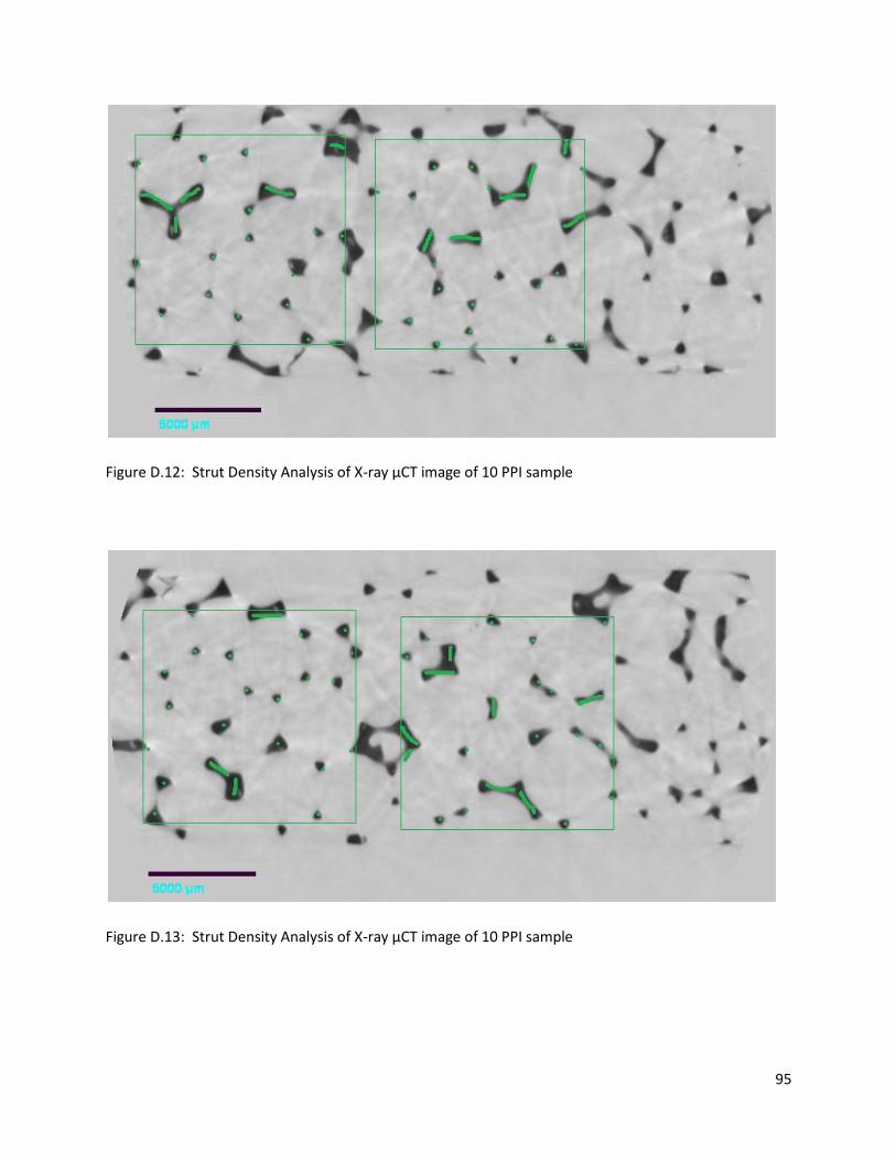
95

Figure D.12: Strut Density Analysis of X-ray μCT image of 10 PPI sample

Figure D.13: Strut Density Analysis of X-ray μCT image of 10 PPI sample

96

Figure D.14: Strut Density Analysis of X-ray μCT image of 10 PPI sample

Figure D.15: Strut Density Analysis of X-ray μCT image of 10 PPI sample

97

Figure D.16: Strut Density Analysis of X-ray μCT image of 10 PPI sample

Figure D.17: Strut Density Analysis of X-ray μCT image of 10 PPI sample

98

Figure D.18: Strut Density Analysis of X-ray μCT image of 10 PPI sample

Figure D.19: Strut Density Analysis of X-ray μCT image of 10 PPI sample

99

Figure D.20: Strut Density Analysis of X-ray μCT image of 10 PPI sample

Figure D.21: Strut Density Analysis of X-ray μCT image of 10 PPI sample

100

20 PPI SAMPLE A

Figure D.22: Strut Density Analysis of X-ray μCT image of 20 PPI sample A

Figure D.23: Strut Density Analysis of X-ray μCT image of 20 PPI sample A

101

Figure D.24: Strut Density Analysis of X-ray μCT image of 20 PPI sample A

102

20 PPI SAMPLE B

Figure D.25: Strut Density Analysis of X-ray μCT image of 20 PPI sample B

Figure D.26: Strut Density Analysis of X-ray μCT image of 20 PPI sample B

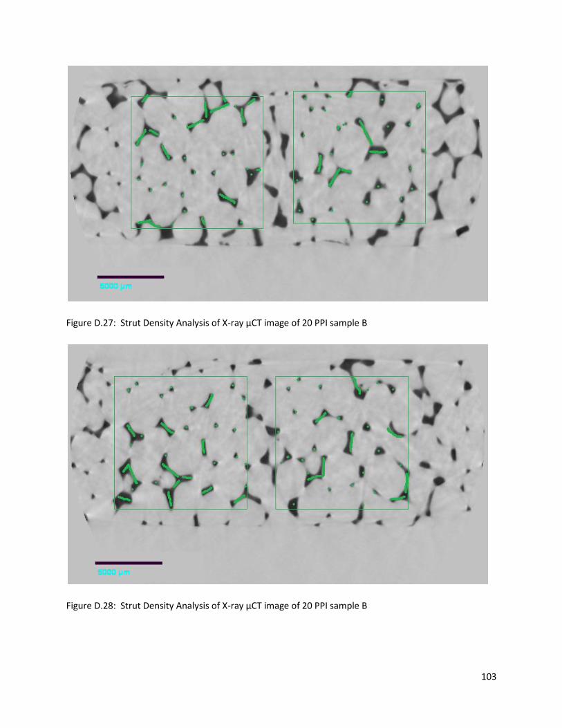
103

Figure D.27: Strut Density Analysis of X-ray μCT image of 20 PPI sample B

Figure D.28: Strut Density Analysis of X-ray μCT image of 20 PPI sample B

104

Figure D.29: Strut Density Analysis of X-ray μCT image of 20 PPI sample B

Figure D.30: Strut Density Analysis of X-ray μCT image of 20 PPI sample B

105

Figure D.31: Strut Density Analysis of X-ray μCT image of 20 PPI sample B

Figure D.32: Strut Density Analysis of X-ray μCT image of 20 PPI sample B

106

Figure D.33: Strut Density Analysis of X-ray μCT image of 20 PPI sample B

Figure D.34: Strut Density Analysis of X-ray μCT image of 20 PPI sample B

107

Appendix E: X-ray μCT Image Analysis—Strut Diameter

Multiple X-ray μCT images were analyzed to determine the average strut diameter. The pink

ellipses were drawn around struts perpendicular to the viewing plane. Both the height and width

of the ellipses were recorded as strut diameters when determining the average.

5 PPI

Figure E.1: Strut Diameter Analysis of X-ray μCT image of 5 PPI sample

Figure E.2: Strut Diameter Analysis of X-ray μCT image of 5 PPI sample

108

Figure E.3: Strut Diameter Analysis of X-ray μCT image of 5 PPI sample

Figure E.4: Strut Diameter Analysis of X-ray μCT image of 5 PPI sample

109

10 PPI

Figure E.5: Strut Diameter Analysis of X-ray μCT image of 10 PPI sample

Figure E.6: Strut Diameter Analysis of X-ray μCT image of 10 PPI sample

110

20 PPI SAMPLE A

Figure E.7: Strut Diameter Analysis of X-ray μCT image of 20 PPI sample A

Figure E.8: Strut Diameter Analysis of X-ray μCT image of 20 PPI sample A

111

Appendix F: Uncertainty Analysis

The propagation equation defined by Kline and McClintock [74] was used to determine the

individual uncertainties for calculated quantities. Statistical uncertainties (two-sigma) were

assigned to FoamView-generated values.

2 2

2 2

22

2 2

2

2 2

1

c

tot c

wet f

tot f

req c

A length width

V A c height

m m m

f

V m

tot ftot f

liq c liq c

L A h

liq liq

u width u length u

u height u A u

u u u

mu u u

VV

h g A g hA gu u u

2

22 2

2 2 2

Zero uncertainty is assumed for densities, surfa

tot c X ray

X ray

liq

liq

L X ray A c l c X ray struts

X ray X ray area

u

struts strutsu l u A u A l u

area area

ce tensions, and gravitational acceleration.

112

Table F.1: Measured Uncertainty

Measured Quantity Nomenclature Bias Error Precision Limit

Length of foam sample length 0.017 in 0.017 in

Width of foam sample width 0.017 in 0.017 in

Height of foam sample height 0.017 in 0.017 in

Height of water column h 0.05 in 0.017 in

Mass of foam (dry and wet) mf, mwet 0.01 g 0.01 g

Table F.2: Statistical Uncertainty

Statistical Quantity Nomenclature Average 2 Standard Deviations

Strut density

5 PPI

10 PPI

20 PPI

(struts/area)

91700 struts/m2

221000 struts/m2

305000 struts/m2

28800 struts/m2

35600 struts/m2

61400 struts/m2

Strut length

5 PPI

10 PPI

20 PPI

lX-ray

1.92 mm

1.49 mm

1.12 mm

1.37 mm

1.03 mm

0.84 mm

Table F.3: Uncertainty Propagation

Quantity Nomenclature Maximum

Uncertainty

Minimum

Uncertainty

Cross sectional area of foam Ac 0.038 in2 0.034 in

2

Volume of foam Vtot 0.14 in3 0.12 in

3

Void fraction 0.0046 0.0026

Average contact length

5 PPI

10 PPI

20 PPI

Ltot

0.132 m

0.188 m

Required contact length

5 PPI

10 PPI

20 PPI

Lreq

0.200 m (91% IPA)

0.199 m (91% IPA)

0.188 m (91% IPA)

0.078 m (water)

0.055 m (water)

0.056 m (water)

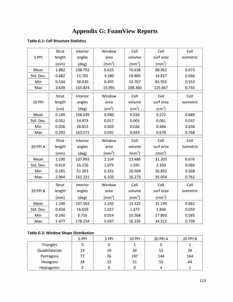
113

Appendix G: FoamView Reports

Table G.1: Cell Structure Statistics

5 PPI

Strut Interior Window Cell Cell Cell

length angles area volume surf area isometric

(mm) (deg) (mm2) (mm3) (mm2) Mean 1.882 108.792 6.625 76.638 98.962 0.673

Std. Dev. 0.682 15.701 3.180 18.805 14.827 0.066

Min 0.534 58.430 0.497 53.767 83.955 0.553

Max 3.639 165.824 15.991 108.360 125.667 0.733

10 PPI

Strut Interior Window Cell Cell Cell

length angles area volume surf area isometric

(cm) (deg) (cm2) (cm3) (cm2) Mean 0.149 108.039 0.040 0.034 0.572 0.689

Std. Dev. 0.052 14.873 0.017 0.005 0.061 0.037

Min 0.036 28.813 0.003 0.026 0.484 0.634

Max 0.293 163.571 0.091 0.043 0.678 0.768

20 PPI A

Strut Interior Window Cell Cell Cell

length angles area volume surf area isometric

(mm) (deg) (mm2) (mm3) (mm2) Mean 1.100 107.993 2.154 13.486 31.203 0.676

Std. Dev. 0.410 16.216 1.075 1.595 2.350 0.060

Min 0.265 51.393 0.331 10.504 26.853 0.568

Max 2.964 161.231 6.103 16.273 35.054 0.761

20 PPI B

Strut Interior Window Cell Cell Cell

length angles area volume surf area isometric

(mm) (deg) (mm2) (mm3) (mm2) Mean 1.140 107.562 2.242 13.325 31.144 0.662

Std. Dev. 0.434 16.659 1.027 1.472 1.836 0.050

Min 0.260 0.716 0.014 10.568 27.803 0.585

Max 2.477 178.234 5.037 16.235 34.512 0.739

Table G.2: Window Shape Distribution

5 PPI 5 PPI 10 PPI 20 PPI A 20 PPI B

Triangles 0 0 1 0 1 Quadrilaterals 19 19 36 52 39 Pentagons 77 76 197 144 164 Hexagons 28 32 51 55 44 Heptagons+ 2 0 0 4 1

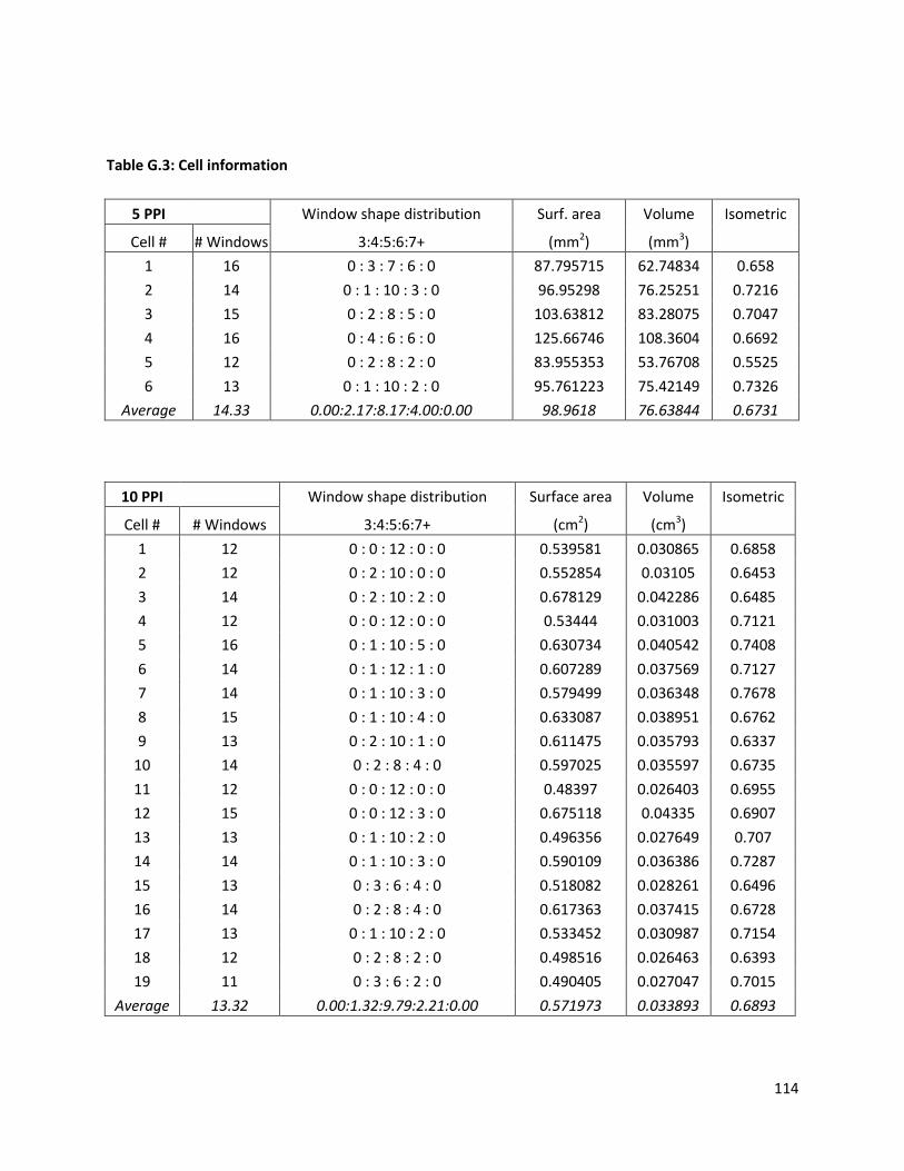
114

Table G.3: Cell information

5 PPI

Window shape distribution Surf. area Volume Isometric Cell # # Windows 3:4:5:6:7+ (mm2) (mm3)

1 16 0 : 3 : 7 : 6 : 0 87.795715 62.74834 0.658 2 14 0 : 1 : 10 : 3 : 0 96.95298 76.25251 0.7216 3 15 0 : 2 : 8 : 5 : 0 103.63812 83.28075 0.7047 4 16 0 : 4 : 6 : 6 : 0 125.66746 108.3604 0.6692 5 12 0 : 2 : 8 : 2 : 0 83.955353 53.76708 0.5525 6 13 0 : 1 : 10 : 2 : 0 95.761223 75.42149 0.7326 Average 14.33 0.00:2.17:8.17:4.00:0.00 98.9618 76.63844 0.6731

10 PPI

Window shape distribution Surface area Volume Isometric Cell # # Windows 3:4:5:6:7+ (cm2) (cm3)

1 12 0 : 0 : 12 : 0 : 0 0.539581 0.030865 0.6858 2 12 0 : 2 : 10 : 0 : 0 0.552854 0.03105 0.6453 3 14 0 : 2 : 10 : 2 : 0 0.678129 0.042286 0.6485 4 12 0 : 0 : 12 : 0 : 0 0.53444 0.031003 0.7121 5 16 0 : 1 : 10 : 5 : 0 0.630734 0.040542 0.7408 6 14 0 : 1 : 12 : 1 : 0 0.607289 0.037569 0.7127 7 14 0 : 1 : 10 : 3 : 0 0.579499 0.036348 0.7678 8 15 0 : 1 : 10 : 4 : 0 0.633087 0.038951 0.6762 9 13 0 : 2 : 10 : 1 : 0 0.611475 0.035793 0.6337 10 14 0 : 2 : 8 : 4 : 0 0.597025 0.035597 0.6735 11 12 0 : 0 : 12 : 0 : 0 0.48397 0.026403 0.6955 12 15 0 : 0 : 12 : 3 : 0 0.675118 0.04335 0.6907 13 13 0 : 1 : 10 : 2 : 0 0.496356 0.027649 0.707 14 14 0 : 1 : 10 : 3 : 0 0.590109 0.036386 0.7287 15 13 0 : 3 : 6 : 4 : 0 0.518082 0.028261 0.6496 16 14 0 : 2 : 8 : 4 : 0 0.617363 0.037415 0.6728 17 13 0 : 1 : 10 : 2 : 0 0.533452 0.030987 0.7154 18 12 0 : 2 : 8 : 2 : 0 0.498516 0.026463 0.6393 19 11 0 : 3 : 6 : 2 : 0 0.490405 0.027047 0.7015 Average 13.32 0.00:1.32:9.79:2.21:0.00 0.571973 0.033893 0.6893

115

20 PPI A

Window shape distribution Surface area Volume Isometric Cell # # Windows 3:4:5:6:7+ (mm2) (mm3)

1 14 0 : 2 : 8 : 4 : 0 29.510557 12.3712 0.6735 2 14 0 : 3 : 8 : 3 : 0 29.038305 11.21198 0.5806 3 13 0 : 4 : 6 : 3 : 0 31.580784 12.75224 0.5839 4 14 0 : 2 : 8 : 4 : 0 35.054295 16.27279 0.6953 5 17 0 : 2 : 10 : 5 : 0 34.134762 15.60678 0.6926 6 13 0 : 1 : 10 : 2 : 0 30.815746 13.52674 0.7072 7 13 0 : 3 : 6 : 4 : 0 34.73048 14.50738 0.5682 8 14 0 : 2 : 8 : 4 : 0 33.004833 15.26167 0.7327 9 13 0 : 1 : 10 : 2 : 0 30.346569 13.15486 0.7003 10 14 0 : 2 : 8 : 4 : 0 32.230419 14.29113 0.6899 11 10 0 : 4 : 6 : 0 : 0 26.85264 10.50406 0.6445 12 15 0 : 4 : 4 : 7 : 0 27.574707 11.87459 0.7606 13 14 0 : 5 : 7 : 2 : 0 32.153728 14.4092 0.7064 14 14 0 : 2 : 8 : 4 : 0 30.257261 12.31871 0.6196 15 14 0 : 2 : 8 : 4 : 0 30.773834 13.79562 0.7386 16 14 0 : 2 : 10 : 2 : 0 31.181232 13.92277 0.7231 Average 13.75 0.00:2.56:7.81:3.38:0.00 31.202509 13.48636 0.6761

20 PPI B

Window shape distribution Surface area Volume Isometric

Cell # # Windows 3:4:5:6:7+ (mm2) (mm3) 1 13 0 : 1 : 10 : 2 : 0 30.389162 13.17633 0.6997

2 12 0 : 3 : 6 : 3 : 0 30.134407 11.89277 0.5846 3 13 0 : 1 : 10 : 2 : 0 30.742638 13.18135 0.6763 4 14 0 : 1 : 10 : 3 : 0 34.251205 14.73156 0.6108 5 15 0 : 2 : 10 : 3 : 0 31.904577 14.21456 0.7037 6 13 0 : 3 : 6 : 4 : 0 30.839428 13.21567 0.6735 7 14 0 : 1 : 10 : 3 : 0 33.812984 15.65369 0.7169 8 13 0 : 2 : 10 : 1 : 0 29.481503 12.19776 0.6567 9 11 0 : 2 : 8 : 1 : 0 30.124838 12.24536 0.6203 10 14 0 : 1 : 10 : 3 : 0 30.629086 13.70393 0.7392 11 12 0 : 2 : 8 : 2 : 0 30.013332 12.14431 0.617 12 14 0 : 2 : 8 : 4 : 0 34.511688 16.23501 0.7252 13 13 0 : 3 : 8 : 2 : 0 31.493046 13.38451 0.6487 14 13 0 : 3 : 6 : 4 : 0 31.031582 13.33614 0.6731 15 12 0 : 4 : 4 : 4 : 0 27.80282 10.56771 0.5877 Average 13.07 0.00:2.07:8.27:2.73:0.00 31.144156 13.32538 0.6622

116

AUTHOR’S BIOGRAPHY

Jessica Bock is the daughter of Don and Rhonda Bock from Benton, Kentucky. She graduated

Magna Cum Laude from the University of Evansville in 2009 with a Bachelor of Science degree

in Mechanical Engineering. Following the completion of her Master of Science Degree in

Mechanical Engineering, Jessica will continue her studies at the University of Illinois at Urbana-

Champaign pursuing her Ph.D.