A GIS Commodity Flow Model for Transportation Policy Analysis:

A Case Study of the Impacts of a Snake River Drawdown

EWITS Research Report Number 18

by

Eric L. Jessup

John Ellis

Department of Agricultural Economics

and

Ken Casavant, EWITS Project Director Washington State University

Department of Agricultural Economics 101 Hulbert Hall

Pullman, WA 99164-6210

EWITS Research Reports: Background and Purpose

This is the eighteenth in a series of reports prepared from the Eastern Washington Intermodal Transportation Study (EWITS). The reports prepared as part of this study provide information to help shape the multimodal network necessary for the efficient movement of both freight and people into the next century. EWITS is a six-year study funded jointly by the Federal government and the Washington State Department of Transportation as a part of the Intermodal Surface Transportation Efficiency Act of 1991. Dr. Ken Casavant of Washington State University is Director of the study. A state-level Steering Committee provides overall direction pertaining to the design and implementation of the project. The Steering Committee includes Jerry Lenzi, Regional Administrator (WSDOT, Eastern Region); Richard Larson (WSDOT, South Central Region); Don Senn (WSDOT, North Central Region); Charles Howard (WSDOT, Planning Manager), and Jay Weber (Douglas County Commissioner). Pat Patterson represents the Washington State Transportation Commission on the Steering Committee. An Advisory Committee with representation from a broad range of transportation interest groups also provides guidance to the study. The following are key goals and objectives for the Eastern Washington Intermodal Transportation Study:

• Facilitate existing regional and state-wide transportation planning efforts.

• Forecast future freight and passenger transportation service needs for eastern Washington.

• Identify gaps in eastern Washington's current transportation infrastructure.

• Pinpoint transportation system improvement options critical to economic

competitiveness and mobility within eastern Washington. For additional information about the Eastern Washington Intermodal Transportation Study or this research report, please contact Ken Casavant at the following address:

Ken Casavant, Project Director Department of Agricultural Economics

Washington State University Pullman, WA 99164-6210

(509) 335-1608

DISCLAIMER The contents of this report reflect the views of the authors, who are responsible for the facts and accuracy of the data presented herein. The contents do not necessarily reflect the official views or policies of the Washington State Department of Transportation or the Federal Highway Administration. This report does not constitute a standard, specification, or regulation.

EWITS PREVIOUS REPORTS NOW AVAILABLE

1. Gillis, William R. and Kenneth L. Casavant. "Linking Transportation System Improvements to New Business Development in Eastern Washington.” EWITS Research Report Number 1. February 1994.

2. Gillis, William R. and Kenneth L. Casavant. "Lessons from Eastern

Washington: State Route Mainstreets, Bypass Routes and Economic Development in Small Towns.” EWITS Research Report Number 2. February 1994.

3. Gillis, William-R. and Kenneth L. Casavant. "Washington State Freight

Truck Origin and Destination Study: Methods, Procedures, and Data Dictionary.” EWITS Research Report Number 3. December 1994.

4. Gillis, William R. and Kenneth L. Casavant. "Major Generators of Traffic on

U.S. 395 North of Spokane: Including Freight Trucks and Passenger Vehicles Crossing the International Border.” EWITS Research Report Number 4. January 1995.

5. Newkirk, Jonathan, Ken Eriksen, and Kenneth L. Casavant. "Transportation

Characteristics of Wheat and Barley Shipments on Haul Roads To and From Elevators in Eastern Washington.” EWITS Research Report Number 5. March 1995.

6. Jessup, Eric and Kenneth L. Casavant. "A Quantitative Estimate of Eastern

Washington Annual Haul Road Needs for Wheat and Barley Movement.” EWITS Research Report Number 6. March 1995.

7. Gillis, William R., Emily Gruss Gillis, and Kenneth L. Casavant.

"Transportation Needs of Eastern Washington Fruit, Vegetable and Hay Industries.” EWITS Research Report Number 7. March 1995.

8. Casavant, Kenneth L. and William R. Gillis. "Importance of U.S. 395 Corridor

For Local and Regional Commerce in South Central Washington.” EWITS Research Report Number 8. April 1995.

9. Gillis, William R., Eric L. Jessup, and Kenneth L. Casavant. "Movement of Freight on Washington's Highways: A Statewide Origin and Destination Study.” EWITS Report Number 9, November 1995.

10. Chase, Robert A. and Kenneth L. Casavant. "Eastern Washington

Transport-Oriented Input Output Study: Technical Report.” EWITS Research Report Number 10. March 1996.

11. Chase, Robert A. Kenneth L. Casavant. "The Economic Contribution of

Transport Industries to Eastern Washington.” EWITS Report Number 11. April 1996.

12. Lee, Nancy S. and Kenneth L. Casavant. "Waterborne Commerce on the

Columbia-Snake.” EWITS Report Number 12. October 1996. 13. Alderson, Lynn C., Kenneth L. Casavant and Eric Jessup. "Transportation

Characteristics and Needs of Forest Products Industries Using Eastern Washington Highways: Part I Economic Structure of the Industry.” EWITS Research Report Number 13. January 1997.

14. Eriksen, Ken and Kenneth L. Casavant. "Impact of North American Free

Trade Agreement (NAFTA) on Washington Highways - Part 1: Commodity and Corridor Projections.” EWITS Research Report Number 14. January 1997.

15. Alderson, Lynn C. and Kenneth L. Casavant. "Transportation Characteristics

and Needs of Forest Products Industries Using Eastern Washington Highways: Part 2 Movement of Raw Logs.” EWITS Research Report Number 15. May 1997.

16. Alderson, Lynn C. and Kenneth L. Casavant. "Transportation Characteristics

and Needs of Forest Products Industries Using Eastern Washington Highways: Part 3 Shipment from Mills.” EWITS Research Report Number 16. May 1997.

17. Alderson, Lynn C. and Kenneth L. Casavant. "Transportation Characteristics

and Needs of Forest Products Industries Using Eastern Washington Highways: Part 4 Commercial Shipments.” EWITS Research Report Number 17. February 1997.

EWITS Previous Working Paper Series Now Available

1. Lee, Nancy and Ken Casavant. "Grain Receipts at Columbia River Grain Terminals.” EWITS Working Paper #1, March 1996.

2. Lenzi, Jerry, Eric Jessup, and Ken Casavant. "Prospective Estimates for

Road Impacts in Eastern Washington from a Drawdown of the Lower Snake River.” EWITS Working Paper #2, March 1996.

3. Ellis, John, Eric Jessup, and Ken Casavant. "Modeling Changes in Grain

Transportation Flows in Response to Proposed Snake River Drawdowns: A Case Study for Eastern Washington.” EWITS Working Paper #3, March, 1996.

4. Painter, Kate and Ken Casavant. "A Comparison of Canadian Versus All

Truck Movements In Washington State With A Special Emphasis On Grain Truck Movements.” EWITS Working Paper #4, March 1996.

5. Jessup, Eric L., John Ellis and Kenneth L. Casavant. "Estimating the Value

of Rail Car Accessibility for Grain Shipments: A GIS Approach.” EWITS Working Paper #5. April 1996.

6. Painter, Kathleen M. and Kenneth L. Casavant. "Truck Movement

Characteristics on Selected Truck Routes in Washington State.” EWITS Working Paper #6. August 1996.

7. Lee, Nancy S. and Kenneth L. Casavant. "Grain Receipts at Columbia River

Grain Terminals, 1980-81 to 1995-96.” EWITS Working Paper #7. January 1997.

8. Jessup, Eric L. and Ken Casavant. "Economic Evaluation of Grain Shipment

Alternatives: A Case Study of the Coulee City and Palouse River Railroad.” EWITS Working Paper #8, March 1997.

Table of Contents Introduction ................................................................................................................... 1 Objective and Approach ............................................................................................... 2 Information Sources ..................................................................................................... 3 Optimization/Modeling Procedure ............................................................................... 5 Results ......................................................................................................................... 12 Disaggregated Wheat Highway Flows....................................................................... 15 Conclusions................................................................................................................. 16 References ................................................................................................................... 29 Appendix A: Arc Macro Language (AML) Program Description ............................ 30 Appendix B: GAMS Model Description .................................................................... 42

List of Figures Figure 1 Eastern Washington Study Area .................................................................. 3 Figure 2 Data and Information Sources ..................................................................... 4 Figure 3 Columbia/Snake River, Elevators, Feedlots, River Ports and Active Rail

Lines in Eastern Washington ....................................................................... 6 Figure 4 Eastern Washington Roads, Highways and Interstates ............................... 7 Figure 5 Eastern Washington Wheat Production Per Acre, by Township/Range....... 8 Figure 6 Eastern Washington Barley Production Per Acre, by Township/Range ....... 9 Figure 7 Optimization Methodology Using GIS and External Optimization Program,

GAMS ........................................................................................................ 10 Figure 8 Optimized Wheat Flows on Eastern Washington Highways (Base Scenario) ......................................................................................... 17 Figure 9 Optimized Wheat Flows on Eastern Washington Highways (No-Barge Scenario) .................................................................................. 18 Figure 10 Optimized Barley Flows on Eastern Washington Highways (Base Scenario) ......................................................................................... 19 Figure 11 Optimized Barley Flows on Eastern Washington Highways (No-Barge Scenario) .................................................................................. 20 Figure 12 Optimized Wheat Highway Flows (Farm to Elevators Without Rail, Base Scenario) .......................................................................................... 21 Figure 13 Optimized Wheat Highway Flows (Farm to Elevators Without Rail, No Barge Scenario).................................................................................... 22 Figure 14 Optimized Wheat Highway Flows (Farm to Elevators With Rail, Base Scenario) .......................................................................................... 23 Figure 15 Optimized Wheat Highway Flows (Farm to Elevators With Rail, No-Barge Scenario) ................................................................................... 24 Figure 16 Optimized Wheat Highway Flows (Farm to River Ports, Base Scenario)... 25 Figure 17 Optimized Wheat Highway Flows (Farm to River Ports, No-Barge Scenario) ................................................................................... 26 Figure 18 Optimized Wheat Highway Flows (Elevator to Elevator and Elevator to River Ports, Base Scenario ........................................................................ 27 Figure 19 Optimized Wheat Highway Flows (Elevator to Elevator and Elevator to River Ports, No-Barge Scenario................................................................. 28

List of Tables Table 1 Wheat Flow Modal Distribution (bushels)................................................... 12 Table 2 Wheat Transportation Costs ...................................................................... 12 Table 3 Wheat Transportation Costs by Origin-Destination Shipment Type ........... 13 Table 4 Barley Flow Modal Distribution................................................................... 14 Table 5 Barley Transportation Costs....................................................................... 14 Table 6 Barley Transportation Costs by Origin-Destination Shipment Type ........... 14 Table A1 Node Type Descriptions............................................................................. 30 Table A2 Origin and Destination File Descriptions .................................................... 30 Table A3 Number of Closest Node Pairs Selected for Each O-D Type..................... 31 Table B1 Description of Input Sets Used in the GAMS Model................................... 42 Table B2 Parameter Description for GAMS Model .................................................... 43

Introduction A myriad of policy debates involving transportation infrastructure, production agriculture, environmentalism, business and trade, and economic welfare are currently underway in the Pacific Northwest. Among these debates are several of specific interests to residents of Eastern Washington where intense wheat and barley production comprise the predominant land use. In addition to heavy concentration of land allocated to production activities, significant economic activity and transportation demands are generated from the production, harvesting and marketing of tremendous grain volumes. These immediate and far reaching ties to residents of Eastern Washington, therefore, create sizeable impacts when external or political stimuli alter the manner of grain production, harvesting, and especially, marketing. Recent national rail mergers and consolidations have targeted several low density rail lines in Eastern Washington for abandonment or sale to shortline operators, creating shipping concerns for producers who rely upon rail transport, highway degradation fears for state transportation officials and highway users, air and noise pollution worries for environmentals, and traffic safety issues for commuters and passenger vehicle operators. Perhaps less problematic, but significant nonetheless, is the seasonal occurrence of grain rail car shortages. The problem arises from the seasonality associated with grain production, harvest and transport. Favorable marketing conditions from September through February encourage producers to ship the majority of grain during these time periods, with considerably less grain movement the remaining six months. Consequently, the quantity of rail cars demanded is considerably larger during this time period. Rail companies, however, invest in equipment (grain cars) with the anticipation of receiving a favorable return on investment, which is difficult if the rail car is not used throughout the year. Thus, to maintain a consistent return on investment, railroad companies attempt to purchase and allocate grain cars on a monthly basis, supplying a base number of rail cars throughout the year rather than supplying cars to meet peak demand. Unfortunately, the demand for grain cars is not evenly distributed throughout the year and a sub-optimal transportation system results as grain is diverted to other, often more costly, modes. Environmental choices also impact grain flows, illustrated by recent attempts to save certain species of salmon from extinction. Regional residents involved with, and affected by, salmon recovery efforts in the Northwest realize the complexities involved with debating the competing interests between fish and man. History has favored man, especially in the Pacific Northwest, where the lock and dam system on the Columbia and Snake rivers has generated an abundance of cheap electricity for businesses and consumers, plentiful water for irrigation in the agricultural sector and cheap, easy access to ocean ports via river barge navigation from Lewiston, Idaho to the ocean.

1

Certain salmon stocks have continued to decrease, to the point where four Snake River Chinook and sockeye species are listed for protection under the federal Endangered Species Act. Since 1980, the Pacific Northwest has spent more than $3 billion trying to save the native fish from extinction, resulting in a multitude of strategies designed to improve salmon survival. One strategy, known as a "river drawdown," involves lowering the water level, thereby increasing river flow and riverine habitat and hopefully, the salmon's odds of survival. Unfortunately, barge traffic would probably cease during drawdown periods, causing potentially adverse impacts on grain farmers, who rely heavily on barge transportation, and on state and local highways as previously river bound commodities take to the highways. Paramount with each of these policy debates is weighing the positive and negative impacts for different constituents and having access to accurate, relevant information. This endeavor works toward that end by constructing a tool that provides information regarding grain producer and transportation infrastructure impacts, for these and other policy discussions. The tool is a transportation optimization model for commodity flows and blends a Geographic Information System (GIS) with a Generalized Algebraic Modeling System (GAMS) optimization package. After describing the model specification and optimization procedure, the model is applied to the river drawdown debate mentioned above.

Objective and Approach This study's purpose is to empirically investigate shipper and transportation infrastructure usage for current Eastern Washington grain flows, and then in the presence of a Snake River drawdown. Changes in transportation flows and shipping cost in the 20 county grain production region of Eastern Washington (see Figure 1) are determined and graphically illustrated. A transportation optimization model, implemented through a Geographical Information System (GIS) incorporating grain movements originating from 695 township centers and passing through over 400 grain elevators en route to final destinations, is descriptively and analytically developed. Impacts on producer's (private) cost of transportation are estimated and transportation flow changes on roads and highways are also presented. Shifts in modal reliance are also provided. Descriptions of the data acquisition and modification procedures are first presented, followed by the transportation optimization model description. The appendices contain detailed technical information about the Arc Macro Language (AML) and GAMS optimization programs, in addition to the program code.

2

lnformation Sources The transportation and marketing system being modeled involves grain movements from production areas in eastern Washington to feedlots and ocean ports for processing, consumption and export. Intermediate destinations, such as elevators and river ports, serve as short (and long) term storage facilities, transfer stations and points of consolidation. Hence, information each component of the system was needed on a common platform to facilitate investigation and analysis. The one common element for each component of the system being modeled is geography. The production areas, elevators, river ports, ocean ports and transportation infrastructure (roads, highways, rail lines, barges) are all connected through geography, creating an ideal environment for a Geographical Information Systems approach.

Figure 1: Eastern Washington Study Area

The GIS coverage’s were constructed primarily from four sources, as illustrated in Figure 2. The Washington State Department of Transportation (WSDOT) provided GIS coverage’s for most county, state, U.S., and Interstate highways, in addition to active rail lines and navigable waterways (see Figure 3). However, these files weren't entirely complete; missing road names and lower density county roads were added from. U.S. Bureau of Census Topologically Integrated Geographic Encoding and Referencing (TIGER) files. WSDOT and TIGER file coverage’s were merged and edited to remove any coinciding arcs or needless road coverage’s, resulting in a complete and non-duplicative coverage of the road and highway transportation network (Figure 4). The WSDOT no longer differentiates between U.S. and state highways, since both are maintained by the state. However, they are presented separately here, corresponding to the TIGER file classifications.

3

Additional information relating to the grain production areas and intermediate destinations (elevators and river ports) was obtained from the Agricultural Soil and Conservation Service (ASCS) and from an elevator survey sent to each of the 400 plus grain elevators in the study area. Detailed data concerning on-farm storage locations and capacities, in addition to acreage and production estimates within each township, were obtained from the ASCS, county assessors, and on site visual inspection (see Figures 5 and 6). Elevator locations, capacities, handling and storage rates, and modal usage were acquired from the survey sent to all elevators in the study area. Over 90% of the surveyed elevators (96% of volume) returned completed questionnaires, providing valuable information on grain movements from production locations to final destinations and the modes utilized in the process. Transport rates for truck shipments were also obtained from the elevator survey. Rail rates were collected from Burlington Northern and Union Pacific, the two class I railroad companies operating in the region, and barge rates were obtained from barge companies operating on the river.

Figure 2: Data and Information Sources

4

Optimization/Modeling Procedure Several GIS software packages designed for transportation modeling and analysis do provide some limited internal optimization features. However, the approach implemented in this analysis utilizes, for flexibility and robustness, an optimization package, which is external to the GIS software. The process being modeled consists of two products (wheat and barley), utilizing multiple modal options and passing through multiple intermediate destinations along several route options, to different final destinations. The complexity associated with this transportation system necessitates a modeling procedure with tremendous flexibility at each phase of the transport process. Therefore, the optimization software used to allocate grain shipments on various modes and routes is called GAMS, an acronym for Generalized Algebraic Modeling System, and is external to the GIS software, Arc Info. The method used to combine the GIS with the minimum cost transportation model is presented in Figure 7. Arc Info is used to generate a collection of minimum distance node combination tables from township centers to elevators, township centers to ports, elevators to elevators, and elevators to river ports (see AML description in Appendix A). These distance tables are then exported to an intermediate program, such as Quattro Pro and Fox Pro, to generate cost coefficients, which are used as an input file in the GAMS optimization model. At each phase of the transportation process, multiple shipment alternatives are incorporated into the optimization model to provide maximum flexibility. Hence, should an optimization run, examining an alternative policy, preclude use of one route, the model still has several routing alternatives from which to choose. Once the set of minimum distance routes are compiled in ArcInfo, and associated cost components incorporated in Quattro Pro, the GAMS optimization software is used to determine the least cost set of shipping routes (see GAMS description in Appendix B). Truck transportation cost coefficients were calculated by estimating a regression equation from elevator survey responses concerning truck transport cost per bushel/mile. A separate equation for wheat (Equation 1) and barley (Equation 2) was estimated. Both equations have the same form where cost per bushel/mile decreases as distance increased initially, but then reaches a point where costs bottom out and then increases with subsequent increases in distance. This reflects the fixed cost of owning a truck and how that amount decreases per bushel/mile as it's spread across more miles. But as distance increases, truck operating expenses increases, causing truck transportation costs per bushel/mile to increase as well. Wheat Truck Cost Per Bushel Mile = .036018 + (.001911 *miles)+(.1518661miles) Equation (1) Barley Truck Cost Per Bushel Mile =.026728 + (.001853 *miles)+ (.1190261miles) Equation (2)

5

Figure 3: Columbia/Snake River, Elevators, Feedlots, River Ports and Active Rail Lines in Eastern Washington

6

Figure 4: Eastern Washington Roads, Highways and Interstates

7

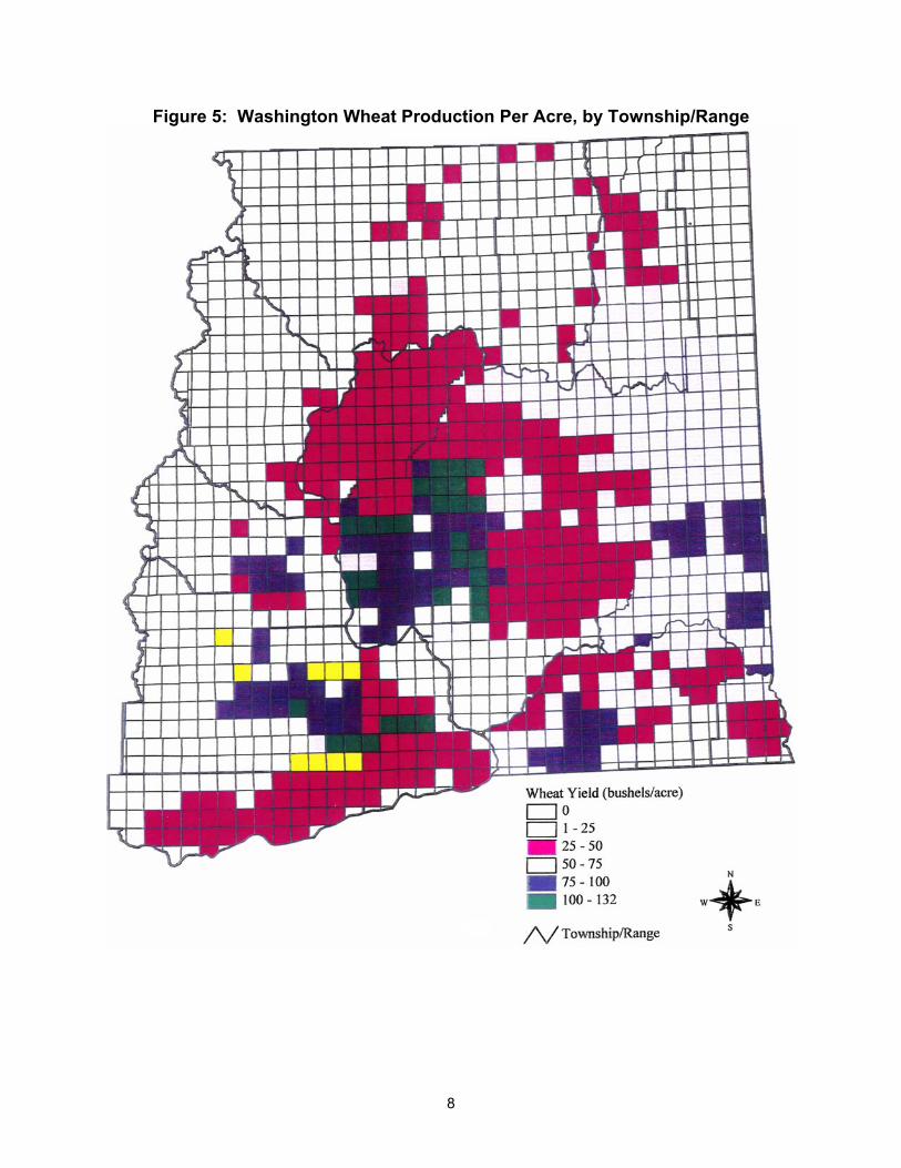
Figure 5: Washington Wheat Production Per Acre, by Township/Range

8

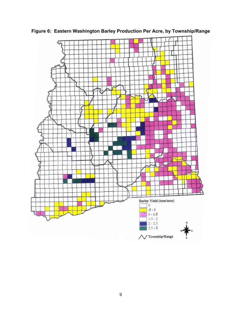
Figure 6: Eastern Washington Barley Production Per Acre, by Township/Range

9

The GAMS model is a linear programming model where the objective is to ship known quantities of grain from production points (township centers) to predefined destinations, while minimizing total transportation cost. The volume of grain supply (and demand) at each township (and final destination) is known. However, the volume of shipments on given routes and modes to reach the final destination is not known. The complexity increases with the introduction of intermediate destinations (elevators and river ports). The movement from production areas is predominately confined to truck shipments, which generally haul directly to river ports for barge transport or to elevators. Once the grain reaches the elevator, several possibilities exist for where and how it may move. If the elevator has rail access, the grain may be loaded onto rail for shipment to final destinations. If the elevator doesn't have rail access, then grain may be transhipped to another elevator with rail access or trucked to a river port for barge transport. The GAMS optimization model incorporates each of these modal shipment and route options at each stage of the grain marketing process, with the decision criteria at each juncture being cost minimization.

Figure 7: Optimization Methodology using GIS and external optimization program, GAMS

The optimization model also includes a variety of constraints, which are constructed to maintain realism in the modeling process. A theoretical optimization system would identify the origin points and the quantities to be shipped, the collection of possible routes on various modes, the cost associated with each route option, and the final destinations, and then allow the linear program to solve for the least cost optimal solution. However, there are capacity constraints at the intermediate destinations which fin-tit the amount of grain, which can be handled at each location. There are also capacity constraints associated with usage of certain modes of transport, particularly for rail shipments. Therefore, to insure that these capacities and others relating to the origins and destinations are not exceeded, the following constraints are included in the optimization model.

10

Supply Balance Equation

=

≤∑n

ij ji 1

S S ∀ j Equation (3)

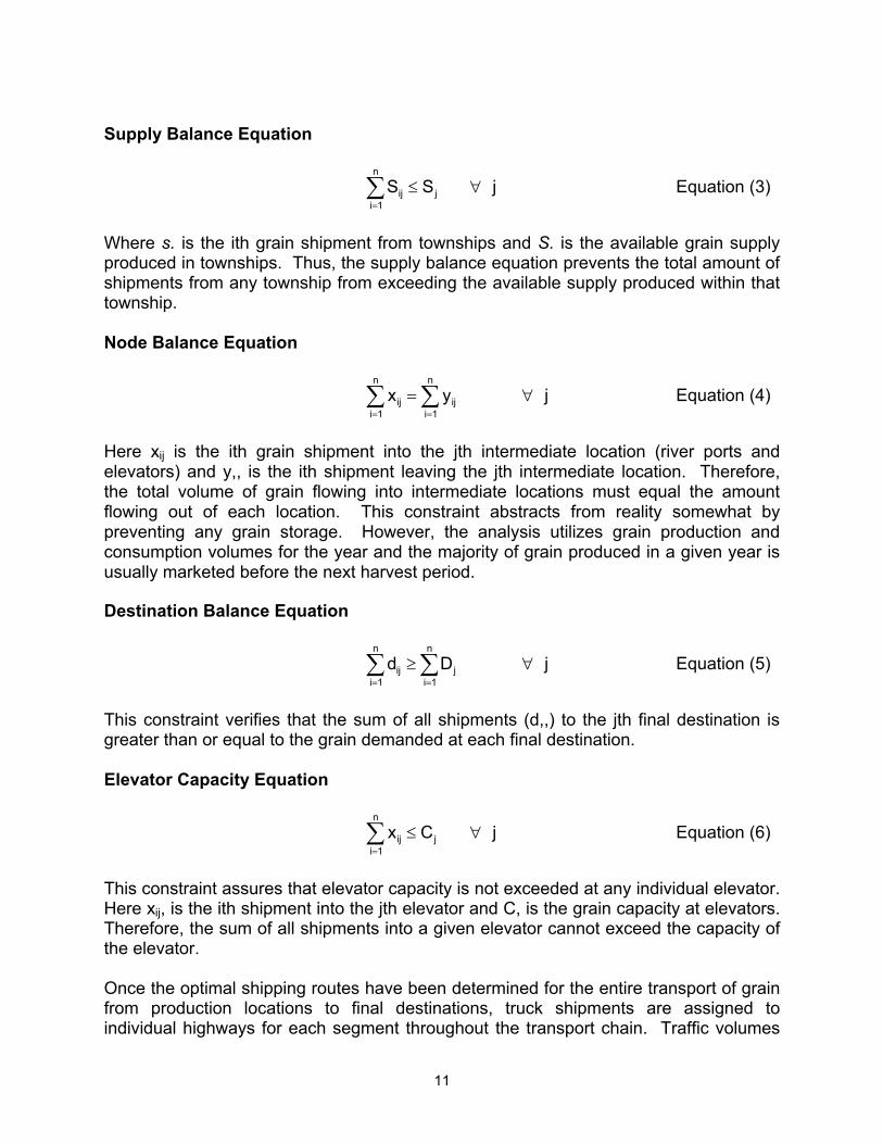
Where s. is the ith grain shipment from townships and S. is the available grain supply produced in townships. Thus, the supply balance equation prevents the total amount of shipments from any township from exceeding the available supply produced within that township. Node Balance Equation

= =

=∑ ∑n n

ij iji 1 i 1

x y ∀ j Equation (4)

Here xij is the ith grain shipment into the jth intermediate location (river ports and elevators) and y,, is the ith shipment leaving the jth intermediate location. Therefore, the total volume of grain flowing into intermediate locations must equal the amount flowing out of each location. This constraint abstracts from reality somewhat by preventing any grain storage. However, the analysis utilizes grain production and consumption volumes for the year and the majority of grain produced in a given year is usually marketed before the next harvest period. Destination Balance Equation

= =

≥∑ ∑n n

ij ji 1 i 1

d D ∀ j Equation (5)

This constraint verifies that the sum of all shipments (d,,) to the jth final destination is greater than or equal to the grain demanded at each final destination. Elevator Capacity Equation

=

≤∑n

ij ji 1

x C ∀ j Equation (6)

This constraint assures that elevator capacity is not exceeded at any individual elevator. Here xij, is the ith shipment into the jth elevator and C, is the grain capacity at elevators. Therefore, the sum of all shipments into a given elevator cannot exceed the capacity of the elevator. Once the optimal shipping routes have been determined for the entire transport of grain from production locations to final destinations, truck shipments are assigned to individual highways for each segment throughout the transport chain. Traffic volumes

11

are then summed for each individual highway arc, since truck shipments starting at different origin points and traveling to different destinations may at times utilize common roads and highways. The truck traffic volumes on roads and highways can then be displayed geographically using either Arclnfo or Arcview. Identification of highway segments with heavy concentrations of truck traffic are then easily identified, in addition to illustrating changes in highway truck traffic flows from different policy scenarios.

Results This portion of the research report presents results from the transportation optimization model concerning modal usage, highway grain flows, and transportation costs for wheat and barley shipments. Two different scenarios are provided including (1) a base scenario depicting current grain flows and (2) a no-barge scenario where barge traffic is eliminated above the Tri-Cities. The total volume of one years grain production (I 994) in this case study is modeled, assuming no extended grain storage. The total volume of wheat shipped via different modes for the base and no-barge Scenarios is 132,836,124 bushels, as depicted in Table 1. Approximately 60 percent of this volume is shipped from production areas to elevators and the remaining 40 percent shipped directly to river ports via truck. This proportion is practically the same for both scenarios, indicating that sizeable amounts of grain would still be trucked directly from production locations to river ports at/or below the Tri-Cities in the absence of river navigation above the Tri-Cities. The largest change in modal usage for wheat shipment in the presence of a river drawdown would be the elevator to river port shipments, which would switch to rail. Elevator to river port shipments decrease 21 percent while elevator to Portland via rail shipments increase by roughly the same percentage. In terms of absolute change, 28.3 million bushels of wheat, would switch from barge to rail. Total transportation costs for all wheat shipments are $65,901,176 and $67,205,885 for the Base and No-Barge Scenarios, respectively, as illustrated in Table 2. The $1.3 million increase in shipper transportation costs amounts to slightly less than 1 cent/bushel, illustrating very little change in region wide shipping charges. However, this represents somewhat of an "averaged" cost per bushel shipping charge indicating that certain shippers would be more adversely impacted than others. Table 1--Wheat Flow Modal Distribution (bushels)

Scenario Truck Rail Barge Total Township

to Elevator

Township to

River Port

Elevator to

Elevator

Elevator to

River Port

Elevator to

Portland

River Port to

Portland

Base 78,098,753 54,737,371 40,276 51,102,369 26,996,384 105,839,740 132,836,124 (Percent of Total)* 59% 41% .03% 38% 20% 80% No-Barge 78,288,953 54,547,171 595,817 22,921,729 55,367,224 77,468,900 132,836,124 (Percent of Total) 59% 41% .4% 17% 42% 58% Absolute Change +190,200 -190,200 +555,541 -28,180,640 +28,370,840 -28,370,840 *Does not sum to 100% due to double counting Table 2--Wheat Transportation Costs Scenario Total Transportation Cost ($) Total Transportation Cost/bu. (cents/bu.) Base 65,901,176 49.61 No-Barge 67,205,885 50.59

12

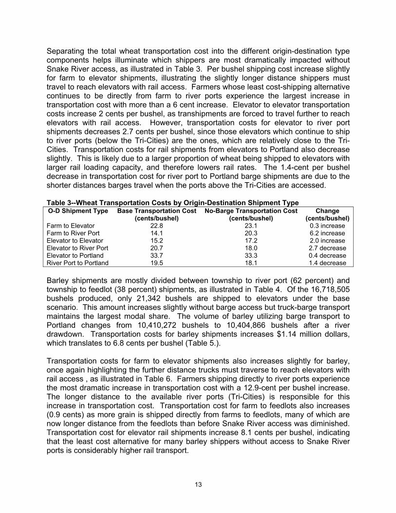
Separating the total wheat transportation cost into the different origin-destination type components helps illuminate which shippers are most dramatically impacted without Snake River access, as illustrated in Table 3. Per bushel shipping cost increase slightly for farm to elevator shipments, illustrating the slightly longer distance shippers must travel to reach elevators with rail access. Farmers whose least cost-shipping alternative continues to be directly from farm to river ports experience the largest increase in transportation cost with more than a 6 cent increase. Elevator to elevator transportation costs increase 2 cents per bushel, as transhipments are forced to travel further to reach elevators with rail access. However, transportation costs for elevator to river port shipments decreases 2.7 cents per bushel, since those elevators which continue to ship to river ports (below the Tri-Cities) are the ones, which are relatively close to the Tri-Cities. Transportation costs for rail shipments from elevators to Portland also decrease slightly. This is likely due to a larger proportion of wheat being shipped to elevators with larger rail loading capacity, and therefore lowers rail rates. The 1.4-cent per bushel decrease in transportation cost for river port to Portland barge shipments are due to the shorter distances barges travel when the ports above the Tri-Cities are accessed. Table 3--Wheat Transportation Costs by Origin-Destination Shipment Type O-D Shipment Type Base Transportation Cost

(cents/bushel) No-Barge Transportation Cost

(cents/bushel) Change

(cents/bushel) Farm to Elevator 22.8 23.1 0.3 increase Farm to River Port 14.1 20.3 6.2 increase Elevator to Elevator 15.2 17.2 2.0 increase Elevator to River Port 20.7 18.0 2.7 decrease Elevator to Portland 33.7 33.3 0.4 decrease River Port to Portland 19.5 18.1 1.4 decrease Barley shipments are mostly divided between township to river port (62 percent) and township to feedlot (38 percent) shipments, as illustrated in Table 4. Of the 16,718,505 bushels produced, only 21,342 bushels are shipped to elevators under the base scenario. This amount increases slightly without barge access but truck-barge transport maintains the largest modal share. The volume of barley utilizing barge transport to Portland changes from 10,410,272 bushels to 10,404,866 bushels after a river drawdown. Transportation costs for barley shipments increases $1.14 million dollars, which translates to 6.8 cents per bushel (Table 5.). Transportation costs for farm to elevator shipments also increases slightly for barley, once again highlighting the further distance trucks must traverse to reach elevators with rail access , as illustrated in Table 6. Farmers shipping directly to river ports experience the most dramatic increase in transportation cost with a 12.9-cent per bushel increase. The longer distance to the available river ports (Tri-Cities) is responsible for this increase in transportation cost. Transportation cost for farm to feedlots also increases (0.9 cents) as more grain is shipped directly from farms to feedlots, many of which are now longer distance from the feedlots than before Snake River access was diminished. Transportation cost for elevator rail shipments increase 8.1 cents per bushel, indicating that the least cost alternative for many barley shippers without access to Snake River ports is considerably higher rail transport.

13

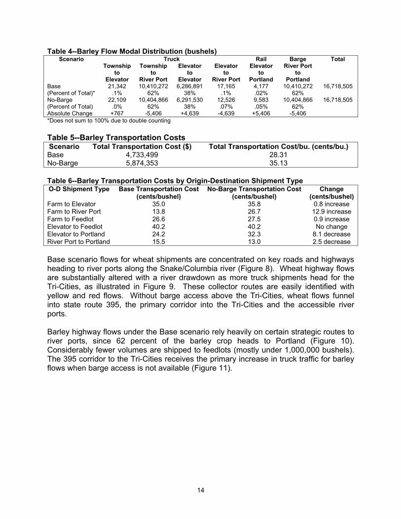
Table 4--Barley Flow Modal Distribution (bushels) Scenario Truck Rail Barge Total

Township to

Elevator

Township to

River Port

Elevator to

Elevator

Elevator to

River Port

Elevator to

Portland

River Port to

Portland

Base 21,342 10,410,272 6,286,891 17,165 4,177 10,410,272 16,718,505 (Percent of Total)* .1% 62% 38% .1% .02% 62% No-Barge 22,109 10,404,866 6,291,530 12,526 9,583 10,404,866 16,718,505 (Percent of Total) .0% 62% 38% .07% .05% 62% Absolute Change +767 -5,406 +4,639 -4,639 +5,406 -5,406 *Does not sum to 100% due to double counting Table 5--Barley Transportation Costs Scenario Total Transportation Cost ($) Total Transportation Cost/bu. (cents/bu.) Base 4,733,499 28.31 No-Barge 5,874,353 35.13 Table 6--Barley Transportation Costs by Origin-Destination Shipment Type O-D Shipment Type Base Transportation Cost

(cents/bushel) No-Barge Transportation Cost

(cents/bushel) Change

(cents/bushel) Farm to Elevator 35.0 35.8 0.8 increase Farm to River Port 13.8 26.7 12.9 increase Farm to Feedlot 26.6 27.5 0.9 increase Elevator to Feedlot 40.2 40.2 No change Elevator to Portland 24.2 32.3 8.1 decrease River Port to Portland 15.5 13.0 2.5 decrease Base scenario flows for wheat shipments are concentrated on key roads and highways heading to river ports along the Snake/Columbia river (Figure 8). Wheat highway flows are substantially altered with a river drawdown as more truck shipments head for the Tri-Cities, as illustrated in Figure 9. These collector routes are easily identified with yellow and red flows. Without barge access above the Tri-Cities, wheat flows funnel into state route 395, the primary corridor into the Tri-Cities and the accessible river ports. Barley highway flows under the Base scenario rely heavily on certain strategic routes to river ports, since 62 percent of the barley crop heads to Portland (Figure 10). Considerably fewer volumes are shipped to feedlots (mostly under 1,000,000 bushels). The 395 corridor to the Tri-Cities receives the primary increase in truck traffic for barley flows when barge access is not available (Figure 11).

14

Disaggregated Wheat Highway Flows Wheat highway flows are further disaggregated for different phases of the wheat marketing process in the remaining Figures (Figures 12-19). Before (base) and after (no-barge) pictures are provided for 1)farm to elevators with rail, 2)farm to elevators without rail, 3)farm to river ports, and 4)elevator to elevator and elevator to river port shipments. Detailed identification of grain flow changes at the disaggregated level reveals patterns not evident for total highway flow changes. Comparing farm to elevators without rail shipments for the base (Figure 12) and no-barge (Figure 13) highlights a noticeable decline in grain flows (in terms of number of farms shipping to an elevator without rail). This seems like a reasonable expectation since elevators without rail loading facilities likely ship to river ports and without river port access, elevators with rail access would be the least cost alternative. Comparison of Figure 14 (farm to elevator with rail, base scenario) and Figure 15 (farm to elevator with rail, no-barge scenario) supports this claim. Several key elevators with rail loading facilities (those with large rail grain loading capacity) become collector points for rail shipments when barge transport ceases above Pasco. Farm to river port grain highway flows also change substantially with fewer local and rural roads east of Pasco receiving much truck traffic, comparing the no-barge scenario (Figure 16) with the base (Figure 17). Without barge access, a few critical highways (US395, SR26, and SR1 7) become collector roads for grain truck traffic to Pasco. Elevator to river port grain movements follow this same pattern with considerably less truck traffic being concentrated on roads leading to river ports above Pasco (Figures 18 and 19).

15

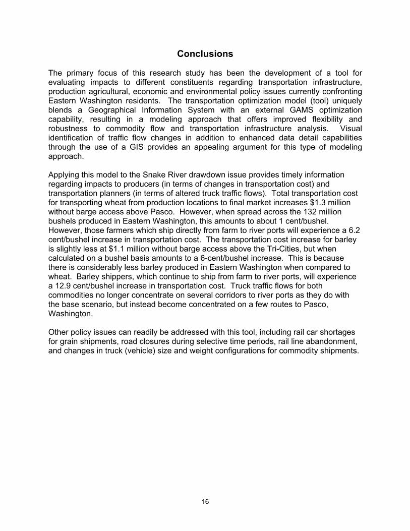
Conclusions The primary focus of this research study has been the development of a tool for evaluating impacts to different constituents regarding transportation infrastructure, production agricultural, economic and environmental policy issues currently confronting Eastern Washington residents. The transportation optimization model (tool) uniquely blends a Geographical Information System with an external GAMS optimization capability, resulting in a modeling approach that offers improved flexibility and robustness to commodity flow and transportation infrastructure analysis. Visual identification of traffic flow changes in addition to enhanced data detail capabilities through the use of a GIS provides an appealing argument for this type of modeling approach. Applying this model to the Snake River drawdown issue provides timely information regarding impacts to producers (in terms of changes in transportation cost) and transportation planners (in terms of altered truck traffic flows). Total transportation cost for transporting wheat from production locations to final market increases $1.3 million without barge access above Pasco. However, when spread across the 132 million bushels produced in Eastern Washington, this amounts to about 1 cent/bushel. However, those farmers which ship directly from farm to river ports will experience a 6.2 cent/bushel increase in transportation cost. The transportation cost increase for barley is slightly less at $1.1 million without barge access above the Tri-Cities, but when calculated on a bushel basis amounts to a 6-cent/bushel increase. This is because there is considerably less barley produced in Eastern Washington when compared to wheat. Barley shippers, which continue to ship from farm to river ports, will experience a 12.9 cent/bushel increase in transportation cost. Truck traffic flows for both commodities no longer concentrate on several corridors to river ports as they do with the base scenario, but instead become concentrated on a few routes to Pasco, Washington. Other policy issues can readily be addressed with this tool, including rail car shortages for grain shipments, road closures during selective time periods, rail line abandonment, and changes in truck (vehicle) size and weight configurations for commodity shipments.

16

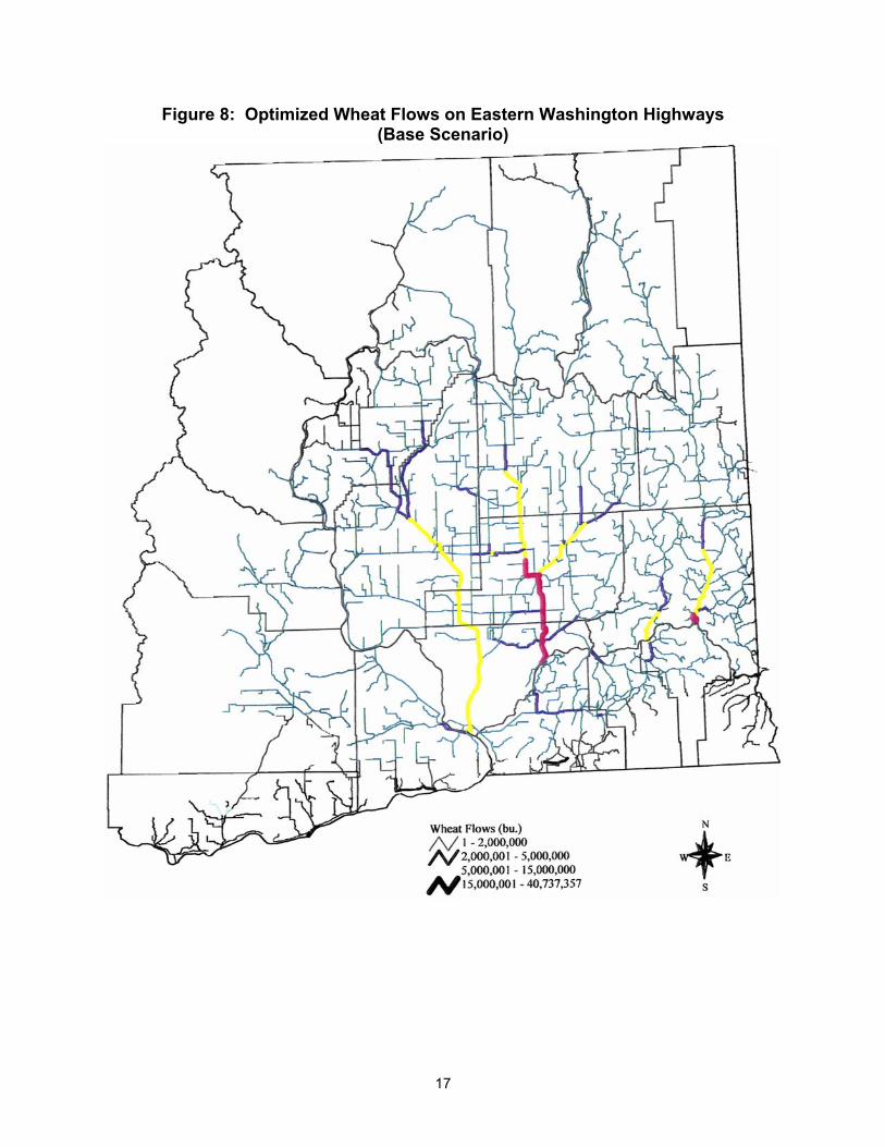
Figure 8: Optimized Wheat Flows on Eastern Washington Highways (Base Scenario)

17

Figure 9: Optimized Wheat Flows on Eastern Washington Highways (Base Scenario)

18

Figure 10: Optimized Wheat Flows on Eastern Washington Highways (Base Scenario)

19

Figure 11: Optimized Wheat Flows on Eastern Washington Highways (Base Scenario)

20

Figure 12: Optimized Wheat Flows on Eastern Washington Highways (Base Scenario)

21

Figure 13: Optimized Wheat Flows on Eastern Washington Highways (Base Scenario)

22

Figure 14: Optimized Wheat Flows on Eastern Washington Highways (Base Scenario)

23

Figure 15: Optimized Wheat Flows on Eastern Washington Highways (Base Scenario)

24

Figure 16: Optimized Wheat Flows on Eastern Washington Highways (Base Scenario)

25

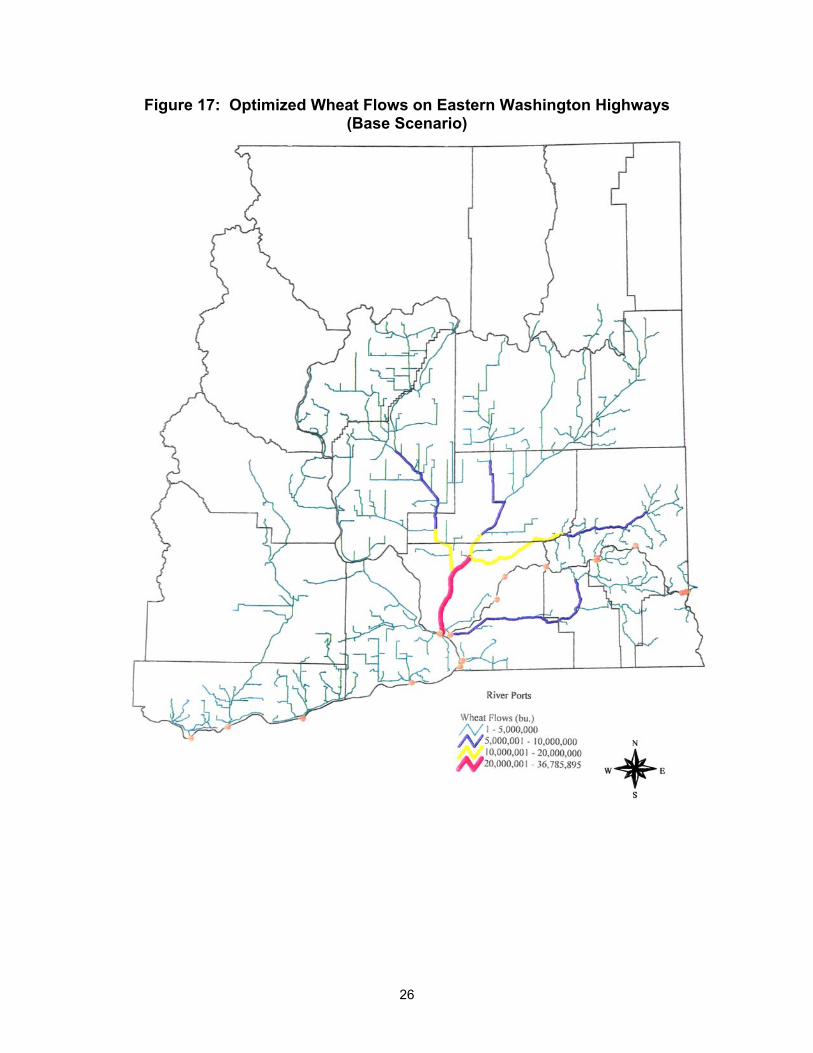
Figure 17: Optimized Wheat Flows on Eastern Washington Highways (Base Scenario)

26

Figure 18: Optimized Wheat Flows on Eastern Washington Highways (Base Scenario)

27

Figure 19: Optimized Wheat Flows on Eastern Washington Highways (Base Scenario)

28

References Kenneth L. Casavant and Richard Mack. "An Economic Evaluation of the Performance

of the Washington State Department of Transportation Grain Train Project.” Prepared for the Washington State Department of Transportation. February, 1996.

William R. Gillis, Eric L. Jessup and Kenneth L. Casavant. "Movement of Freight on

Washington's Highways: A Statewide Origin and Destination Study.” Eastern Washington Intermodal Transportation Study Report #9. Washington State University/Washington State Department of Transportation, November 1995.

Jonathon R. Newkirk and Ken A. Eriksen. "Transportation Characteristics of Wheat and

Barley Shipments on Haul Roads To and From Elevators in Eastern Washington.” Eastern Washington Intermodal Transportation Study #5. Washington State University/Washington State Department of Transportation, March, 1995.

Freight Services Incorporated (FSI). "A Review of Eastern Washington Grain Car

Supply, Impacts on Shipping, and Need for Governmental Intervention.” Prepared for the Washington State Department of Transportation. September, 1993.

29

Appendix A

Arc Macro Language (AML) Program Description The route generation process begins with a parent coverage (in this AML the parent coverage is bigcov) where the collection of all arcs and nodes are contained. An arc is a series of points that start and end with a node. A node is an intersection point where two or more arcs meet. Nodes are also classified into numeric categories based on common features or characteristics. This model is concerned with generating grain-shipping routes on highways between certain nodes of interest, which are provided in Table Al. Table A1--Node Type Descriptions Node Type Geographic Description Origin/Destination Type

2 On-farm grain storage location Origin Point 3 Elevator without rail loading facilities Intermediate Destination 4 Elevator with rail loading facilities Intermediate Destination 5 River Port Intermediate Destination 6 Feedlot Final Destination 8 Township Center Origin Point

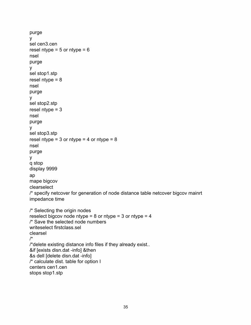
Node types 2 and 8 are considered origin nodes in Table Al but in the current model specification only node types 8 are used as origin shipping points. Future analysis may require using node type 2 instead of node type 8 (or some combination of the two) as origin points in the model. Also notice that the final destination "Portland" is not listed in the table. This is because Portland is accessed via river barge or rail and not truck shipment. The model begins by first checking to see if important files, which are generated in the model, already exist and then deletes them. This is to prevent problems overwriting files should the program abort before completion. Then beginning on page 35, three origin files (stopl.stp, stop2.stp, and stop3.stp) and three destination files (cen1.cen, cen2.cen, and cen3.cen) are generated from the parent coverage (bigcov) node attribute table. These origin and destination files separate node attribute information to allow pairing of different origin and destination node combinations of interest. The node types contained in each .stp and .cen file are provided in Table A2. Table A2--Origin and Destination File Description

Origin File Node Type Destination File Node Type stop1.stp 8 cen1.cen 3 and 4 stop2.stp 3 cen2.cen 4 stop3.stp 3, 4 and 8 cen3.cen 5 and 6

After these stop and cen files are created the netcover is specified for the parent coverage bigcov as mainrt. The netcover command simply specifies the line coverage containing the network and the output route system to which paths, tours and allocations are written. The impedance variable is time, which is used to identify which origin, and destination node pairs are selected. The stop and cen files in Table A2 are

30

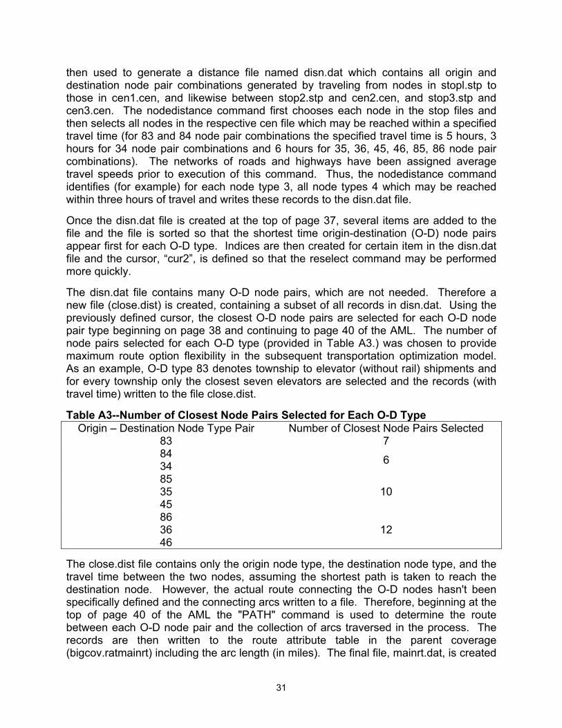
then used to generate a distance file named disn.dat which contains all origin and destination node pair combinations generated by traveling from nodes in stopl.stp to those in cen1.cen, and likewise between stop2.stp and cen2.cen, and stop3.stp and cen3.cen. The nodedistance command first chooses each node in the stop files and then selects all nodes in the respective cen file which may be reached within a specified travel time (for 83 and 84 node pair combinations the specified travel time is 5 hours, 3 hours for 34 node pair combinations and 6 hours for 35, 36, 45, 46, 85, 86 node pair combinations). The networks of roads and highways have been assigned average travel speeds prior to execution of this command. Thus, the nodedistance command identifies (for example) for each node type 3, all node types 4 which may be reached within three hours of travel and writes these records to the disn.dat file. Once the disn.dat file is created at the top of page 37, several items are added to the file and the file is sorted so that the shortest time origin-destination (O-D) node pairs appear first for each O-D type. Indices are then created for certain item in the disn.dat file and the cursor, “cur2”, is defined so that the reselect command may be performed more quickly. The disn.dat file contains many O-D node pairs, which are not needed. Therefore a new file (close.dist) is created, containing a subset of all records in disn.dat. Using the previously defined cursor, the closest O-D node pairs are selected for each O-D node pair type beginning on page 38 and continuing to page 40 of the AML. The number of node pairs selected for each O-D type (provided in Table A3.) was chosen to provide maximum route option flexibility in the subsequent transportation optimization model. As an example, O-D type 83 denotes township to elevator (without rail) shipments and for every township only the closest seven elevators are selected and the records (with travel time) written to the file close.dist. Table A3--Number of Closest Node Pairs Selected for Each O-D Type

Origin – Destination Node Type Pair Number of Closest Node Pairs Selected 83 7 84 34 6

85 35 45

10

86 36 46

12

The close.dist file contains only the origin node type, the destination node type, and the travel time between the two nodes, assuming the shortest path is taken to reach the destination node. However, the actual route connecting the O-D nodes hasn't been specifically defined and the connecting arcs written to a file. Therefore, beginning at the top of page 40 of the AML the "PATH" command is used to determine the route between each O-D node pair and the collection of arcs traversed in the process. The records are then written to the route attribute table in the parent coverage (bigcov.ratmainrt) including the arc length (in miles). The final file, mainrt.dat, is created

31

from the bigcov.ratmainrt file but first two additional files (orig.dat and dest.dat) must be created so that the items contained in each file may be joined with mainrt.dat. The orig.dat and dest.dat files are created by first selecting certain items from the bigcov.nat file and writing the records to each respective file. Orig.dat contains node information about all origin nodes and dest.dat contains information about all destination nodes. The item names in both files are changed to names that are more descriptive and consistent across files and then these two files, in addition to close. dist, are joined with mainrt.dat with the use of the "JOINITEM" command. As previously mentioned, the file mainrt.dat is created from the route attribute table bigcov.ratmainrt, with some added items and new names. Both files are a record of all routes and the length (in miles) of all combined arcs that comprise a given route. Mainrt.dat is then used to create the input sets in the GAMS transportation optimization model. Routes are divided into separate O-D node type pairings (83, 84, 85, 86, 34, 35, 36, 45, 46) and the distances are multiplied by per bushel/mile cost coefficients to determine the cost associated with traversing each route. Routes that end at an elevator or river port have storage and handling charges added to the cost of each route. These routes (and their associated cost) are the set of all potential routes from which the transportation model has to choose in determining the least cost optimal solution, given certain constraints on grain supply availability, elevator capacity, and quantity demanded at each final destination. Once the transportation optimization model has allocated grain volumes to specific routes, some additional steps are necessary to link the grain flows to individual highway arcs. Grain volumes from the GAMS model output corresponds to routes that are referenced using unique origin and destination site names which are separated by a period (for example, TR653138.EL46E representing a township to elevator (83) route). However, instead of having a name to represent routes, numbers are assigned to specific routes in ArcInfo indicating that the GAMS output must be linked (via the O-D name) with the mainrt.dat file to query those routes from mainrt.dat with positive grain flows. This newly created file (named new.dat for illustration) contains all the information of mainrt.dat, in addition to grain flows for each route. This file is then joined with the section table bigcov.secmainrt to add the grain flows for each route to the individual highway arcs comprising a route. After the grain volumes are added to individual highway arcs, the "FREQUENCY" command is used to sum over all routes the grain volume utilizing each highway arc. In many situations, a given highway arc will be common to several routes. Hence, all grain shipments, which utilize an arc, must be summed to represent the total volume passing over that particular arc. The file that is generated (specified when executing the "FREQUENCY" command) with this procedure contains the aggregated grain flows on each arc. Joining this table with the arc attribute table bigcov.aat allows display of the, grain flows throughout the entire highway network.

32

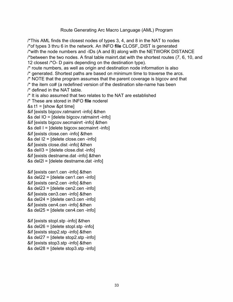
Route Generating Arc Macro Language (AML) Program

/*This AML finds the closest nodes of types 3, 4, and 8 in the NAT to nodes /*of types 3 thru 6 in the network. An INFO file CLOSF,.DIST is generated /*with the node numbers and -IDs (A and B) along with the NETWORK DISTANCE /*between the two nodes. A final table mainrt.dat with the shortest routes (7, 6, 10, and 12 closest /*O- D pairs depending on the destination type). /* route numbers, as well as origin and destination node information is also /* generated. Shortest paths are based on minimum time to traverse the arcs. /* NOTE that the program assumes that the parent coverage is bigcov and that /* the item co# (a redefined version of the destination site-name has been /* defined in the NAT table. /* It is also assumed that two relates to the NAT are established /* These are stored in INFO file noderel &s t1 = [show &pt time] &if [exists bigcov.ratmainrt -info] &then &s del IO = [delete bigcov.ratmainrt -info] &if [exists bigcov.secmainrt -info] &then &s dell I = [delete bigcov.secmainrt -info] &if [exists close.cen -info] &then &s del I2 = [delete close.cen -info] &if [exists close.dist -info] &then &s deII3 = [delete close.dist -info] &if [exists destname.dat -info] &then &s del2l = [delete destname.dat -info]

&if [exists cen1.cen -info] &then &s del22 = [delete cen1.cen -info] &if [exists cen2.cen -info] &then &s del23 = [delete cen2.cen -info] &if [exists cen3.cen -info] &then &s del24 = [delete cen3.cen -info] &if [exists cen4.cen -info] &then &s del25 = [delete cen4.cen -info]

&if [exists stopl.stp -info] &then &s del26 = [delete stopl.stp -info] &if [exists stop2.stp -info] &then &s del27 = [delete stop2.stp -info] &if [exists stop3.stp -info] &then &s del28 = [delete stop3.stp -info]

33

&if [exists stop4.stp'-infol &then &s del29 = [delete stop4.stp –info &messages &off tables sel bigcov.nat calc bigcov-id = bigcov# q stop /* Create the base file from the NAT for use with the nodedistance command in ap pullitems bigcov.nat cen1.cen bigcov-id ntype end /* Create stops and centers files for 3 options /* Stops files are used for origins and centers files for the destinations /* /* stops file ntypes centers file ntype time limit /* /* stopl.stp 8 cen1.cen 3,4 3 hrs /* stop2.stp 3 cen2.cen 4 3 hrs /* stop3.stp 3,4,8 cen3.cen 5,6 4hrs /* /* Assumes ntype entity

2 on farm storage location 3 elev 4 elev with rail 5 port 6 feedlot 8 township center

tables copy cen1cen stopl.stp copy cen1cen stop2.stp copy cen1cen stop3.stp copy cen1cen cen2.cen copy cen1cen cen3.cen sel cen1cen resel ntype = 3 or ntype 4 nsel purge y sel cen2.cen resel ntype = 4 nsel

34

purge y sel cen3.cen resel ntype = 5 or ntype = 6 nsel purge y sel stop1.stp resel ntype = 8 nsel purge y sel stop2.stp resel ntype = 3 nsel purge y sel stop3.stp resel ntype = 3 or ntype = 4 or ntype = 8 nsel purge y q stop display 9999 ap mape bigcov clearselect /* specify netcover for generation of node distance table netcover bigcov mainrt impedance time /* Selecting the origin nodes reselect bigcov node ntype = 8 or ntype = 3 or ntype = 4 /* Save the selected node numbers writeselect firstclass.sel clearsel /* /*delete existing distance info files if they already exist.. &if [exists disn.dat -info] &then &s dell [delete disn.dat -info] /* calculate dist. table for option I centers cen1.cen stops stop1.stp

35

nodedistance stops centers disn.dat 5 network ids /* calculate dist. table for option 2 centers cen2.cen stops stop2.stp nodedistance stops centers disn2.dat 3 network ids /* calculate dist. table for option 3 centers cen3.cen stops stop3.stp nodedistance stops centers disn3.dat 6 network ids &messages &on /* join 4 distance tables together using arcedit &data arc arcedit edit disn.dat info get disn2.dat get disn3.dat save disn.dat y y y q &end &messages &off &data arc tables /* Add items for origin ntype, dest. ntype, and combination additem disn.dat ot 4 5 b additem disn.dat dt 4 5 b additem disn.dat odt 4 5 b additem disn.dat oco# 2 2 c additem disn.dat dco# 2 2 c relate restore noderel sel disn.dat calc ot = orel//ntype calc dt = drel//ntype calc odt = 10 * ot + dt move orel//co# to oco# move drel//co# to dco# /* Put table in correct order so that least time elev are in the table /* first. sort odt bigcov#a network q stop &end /* Create indices on selected items so that reselect perform more quickly &data arc

36

indexitem disn.dat bigcov#a indexitem disn.dat bigcov#b indexitem disn.dat dt q &end /* open the nodes in the first class readselect firstclass.sel &s cnt [extract I [show select bigcov node]] cursor cur2 declare disn.dat info &s t2 = [show &pt time] &format 3 relate restore noderel &do i = I &%cnt% /*set the record numbers for the class1 nodes &s mnhl [show select bigcov node %i% item bigcov#] &s ontype [show select bigcov node %i% item ntype] &s oname = [show select bigcov node %i% item co#

&lv oname clearsel bigcov node /*find those node pair distances of interest /* for dest type 3 /* If the od pair is type 33 (elev to elev) writes only for those /* pairs within the same firm. Does not limit the write to only the /* 3 closest for od pairs of this type. Other od pair types (i.e., 83) /* are written for the 3 closest pairs to a given origin node. aselect disn.dat info reselect disn.dat info bigcov#a = %mnhl% reselect disn.dat info dt = 3 &if [value ontype] <> 3 &then &do /*find the 7 closest nodes and write to INFO file appended &s num1 = [extract I [show select disn.dat info]] &s num2 = [min 7 %num1 %] cursor cur2 open

&do k = I &to %num2% inf6file disn.dat info close.dist # append cur cur2 next &end cursor cur2 close

&end /* For od type 33 pairs, write out all entries within a given firm &else &do

reset disn.dat info dco# co [quote %oname%]

37

&s num1 = [extract 1 [show select disn.dat info]] &if %num1% ge 1 &then infofile disn.dat info close.dist # append &end clearsel /*find those node pair distances of interest /* for dest type 4 aselect disn.dat info reselect disn.dat info bigcov#a = %mnhl% reselect disn.dat info dt = 4 /*find the 6 closest nodes and write to INFO file appended &s num1 = [extract I [show select disn.dat info]] &s num2 = [min 6 %num I%] cursor cur2 open &do k = I &to O/onum2% infofile disn.dat info close.dist # append cur cur2 next &end cursor cur2 close clearsel /*find those node pair distances of interest /* for dest type 5 aselect disn.dat info reselect disn.dat info bigcov#a = %mnhl% reselect disn.dat info dt = 5 /*find the 10 closest nodes and write to INFO file appended &s num1 = [extract I [show select disn.dat info]] &s num2 = [min IO %num I%] cursor cur2 open &do k = I &to %num2% infofile disn.dat info close.dist # append cur cur2 next &end cursor cur2 close clearsel /*find those node pair distances of interest /* for dest type 6 aselect disn.dat info reselect disn.dat info bigcov#a = %mnhl% reselect disn.dat info dt = 6 /*find the 12 closest nodes and write to INFO file appended &s num1 = [extract I [show select disn.dat info]] &s num2 = [min 12 %num I%]

38

cursor cur2 open &do k = I &to %num2% infofile disn.dat info close.dist # append cur cur2 next &end cursor cur2 close clearsel readselect firstclass.sel &end /* end of big loop to create file close.dist /* Time to generate the route system for those records in close.dist &s t3 = [show &pt time] clearsel relate restore noderel cursor curl declare close.dist ro cursor curl open &do &while %:cur1.AML$NEXT% &s x = [VALUE :cur1.bigcov-ida] &s y = [VALUE :cur1.bigcov-idb] &s w = [VALUE :cur1.orel//ntype * 10 + [VALUE :cur1.drel//ntype] path %x% %y% end %w% cursor curl next &end cursor curl close /* draw the resulting route system /* routelines bigcov mainrt 6 /* &sv done [QUERY 'Hit return to continue' .FALSE.] /* quit ap q /* Tack the arclength onto the RAT file routestats bigcov mainrt arclength end end /* delete old files if they exist &if [exists orig.dat -info] &then &s del5 = [delete orig.dat -info] &if [exists dest.dat -info] &then &s del6 = [delete dest-dat -info] &if [exists mainrt.dat -info] &then &s del7 = [delete mainrt-dat -info] /* Pull selected items from the NAT to create an orig and dest file to /* tack onto the RAT file and create the file mainrt.dat

39

pullitems bigcov.nat orig.dat bigcov# ntype site-name county ctr end /* additem %rt%# to close.dist so can join to RAT tables copy orig.dat dest.dat additem close.dist mainrt# 4 5 b dropitem close.dist bigcov-ida bigcov-idb sel close.dist calc mainrt# = $recno /* 143 reduce the orig.dat to only origin nodes and alter item names sel orig.dat resel ntype = 3 or ntype 4 or ntype 8 nsel purge y alter bigcov# bigcov#a,,,, alter ntype ontype,,,, alter site_name osn,,,, alter county ocounty,,,, alter ctr octr,,,, /* reduce the dest.dat to only destination nodes and alter item names sel dest.dat resel ntype ge 3 and ntype le 6 nsel purge y alter bigcov# bigcov#b,,,, alter ntype dntype,,,, alter site_name dsn,,,, alter county

40

dcounty,,, alter ctr dctr,,,, copy bigcov.ratmainrt mainrt-dat q stop /* 177 join close.dist to the copied RAT and then join /* the origin and destination node information joinitem mainrt.dat close.dist mainrt.dat mainrt# arclength joinitem mainrt.dat orig.dat mainrt.dat bigcov#a network joinitem mainrt.dat dest.dat mainrt.dat bigcov#b octr dropitem mainrt.dat mainrt.dat ot dropitem mainrt.dat mainrt.dat dt dropitem mainrt.dat mainrt.dat odt tables sel mainrt.dat list &messages &on N q stop &s t4 = [show &pt time] &lv t1 t2 t3 t4

41

Appendix B

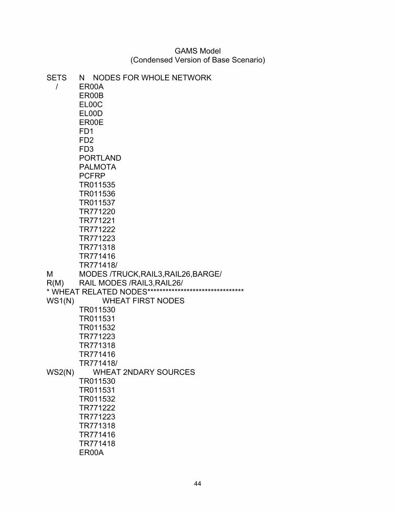
GAMS Model Description The transportation optimization model, which allocates grain shipments throughout the transportation network, utilizes the Generalized Algebraic Modeling System (GAMS). A condensed version of the actual program used to model the base scenario follows this brief description. GAMS models have a very unique structure and format. Large, complex models can- be represented in a very compact, understandable language and changes easily made. Initially, however, they can be confusing without some basic explanation. The transportation optimization model begins by defining all input SETS to be used in the model. In this model there are 36 input sets, which are described in Table B 1. These input sets provide the basic building blocks for the remainder of the GAMS program since any algebraic manipulations will generally involve these input sets. Table B1--Description of Input Sets Used in the GAMS Model Set Name Description

N Every node in the transportation network. Includes all elevators, feedlots, river ports, grain production townships, and Portland.

M All available transport modes including: truck, 3-car rail, 26-car rail, and barge.

R(M) Rail modes including: 3-car rA and 26-car rail. WS1(N) Every township/range in Eastern Washington with positive wheat

production. WS2(N) WS1(N) in addition to all elevators which handle wheat and river ports, WINT(N) All elevators, which handle wheat and river ports. ELEV(N) Elevators without rail loading facilities. RELEV(N) Elevators with rail loading facilities. WD(N) The only wheat destination node: Portland. WD2(N) All elevators, river ports and Portland. IPORT(N) The 17 river ports located on the Snake/Columbia river system. BS1(N) Every township/range in Eastern Washington with positive barley

production. BS2(N) BS1 (N) in addition to all elevators which handle barley and river ports. BINT(N) Elevators which handle barley and river ports. BFD(N) All feedlots in Eastern Washington which use barley, BINT2(N) All elevators, which handle wheat, river ports, and feedlots. BD(N) Feedlots and Portland. BD2(N) Elevators handling wheat, river ports, feedlots and Portland. CAPSET(N) All elevators. C01(N) Every township/range in Adams county with positive wheat production. C05(N) Every township/range in Benton county with positive wheat production. C07(N) Every township/range in Chelan county with positive wheat production. C13(N) Every township/range in Columbia county with positive wheat production. C17(N) Every township/range in Douglas county with positive wheat production. C21(N) Every township/range in Franklin county with positive wheat production.

42

C23(N) Every township/range in Garfield and Asotin counties with positive wheat production.

C25(N) Every township/range in Grant county with positive wheat production. C37(N) Every township/range in Kittitas county with positive wheat production. C39(N) Every township/range in Klickitat county with positive wheat production. C43(N) Every township/range in Lincoln county with positive wheat production. C47(N) Every township/range in Okanogan county with positive wheat production.C63(N) Every township/range in Spokane and Ferry counties with positive wheat

production. C65(N) Every township/range in Stevens county with positive wheat production. C71(N) Every township/range in Walla Walla county with positive wheat

production. C75(N) Every township/range in Whitman county with positive wheat production. C77(N) Every township/range in Yakima county with positive wheat production. After all input sets have been defined, the data is then declared by using the 'TABLES" command. Two large tables are declared: WARCS and BARCS for wheat and barley arcs, respectively. Within each table is a listing of all origin-destination node pairs and the cost coefficient to travel between the two nodes. Each table has truck, 3-car rail, 26-car rail, and barge shipment options. All route combinations generated in the previous AML program are included in the tables, WARCS and BARCS. The next segment of the model involves defining the parameters and assigning the values for each set of parameters. The 'PARAMETER" command is used here to define the nine parameters described in Table B2. Table B2--Parameter Description for GAMS model

Parameter Description WSUP(N) Wheat supply (in bushels) produced in each township/range. BSUP(N) Barley supply (in bushels) produced in each township/range. RAILCAPW(N) Historical volume of wheat shipped on rail from elevators. RAILCAPB(N) Historical volume of barley shipped on rail from elevators. RAILCAPW2(N) Variable used to scale RAILCAPW(N). RAILCAPB2(N) Variable used to scale RAILCAPB(N). CAPRHS(N) Elevator grain capacity, in bushels. CAPRHS2(N) Variable used to scale elevator grain capacity. BDEM(N) Volume of barley demand at each feedlot and Portland. All variables and equations in the model are then defined. The variables are all unknowns to be determined in the optimization process such as grain flows on individual arcs and total cost. The variables in combination with the input sets and parameters defined earlier are the ingredients used to construct the equations. The variables and equations are described in the GAMS program. The final step is to specify how the model is to be solved which simply involves submitting the 'SOLVE" statement, instructing the model to minimize total transport cost using a linear program. Following this statement are several loops where the display of grain flows are separated into several origin-destination pairs for analysis.

43

GAMS Model (Condensed Version of Base Scenario)

SETS N NODES FOR WHOLE NETWORK / ER00A ER00B EL00C EL00D ER00E FD1 FD2 FD3 PORTLAND PALMOTA PCFRP TR011535 TR011536 TR011537 TR771220 TR771221 TR771222 TR771223 TR771318 TR771416 TR771418/ M MODES /TRUCK,RAIL3,RAIL26,BARGE/ R(M) RAIL MODES /RAIL3,RAIL26/ * WHEAT RELATED NODES******************************** WS1(N) WHEAT FIRST NODES TR011530 TR011531 TR011532 TR771223 TR771318 TR771416 TR771418/ WS2(N) WHEAT 2NDARY SOURCES TR011530 TR011531 TR011532 TR771222 TR771223 TR771318 TR771416 TR771418 ER00A

44

EL00C EL00D ER00E ER00F ER00G EL00H ER00K ER71J ER71M EL710 PALMOTA PCFRP PCFPGG PLYONSF PWINDUST PCLARK PUMATIILL PROOSVLT PBIGGS PDALLES/ WINT(N) WHEAT INTERMEDIATE NODES EROOA / ER00A EL00C ER00K EL01B ER01C EL02A ER02B ER02F EL71O PALMOTA PCFRP PCFPGG PLYONSF PWINDUST PWALLULA PPTKELLY PUMATILL PROOSVLT PBIGGS PDALLES/ ELEV(N) ELEVATORS WITH NO RAIL / EL00C EL00D EL00H EL01B

45

EL671 EL67J EL67K EL67L EL67V EL67X EL71G EL71O/ RELEV(N) WHEAT ELEVATORS WITH RAIL / ER00A ER00B ER00E ER00F ER00G ER71A ER71D ER71F ER711 ER71J ER71M/ WD(N) WHEAT DEST NODE /PORTLAND/ WD2(N) WHEAT 2NDARY DESTINATIONS / ER00A EL00C EL00D ER00E ER00F ER00G EL00H ER00K EL01B ER01C ER71M EL710 PALMOTA PCFRP PCFPGG PLYONSF PWINDUST PCLARK PUMATILL PROOSVLT PBIGGS PDALLES PORTLAND/ IPORT(N) INTERMEDIATE PORTS

46

/ PALMOTA PCFRP PCFPGG PLYONSF PWINDUST PCLARK PWILMA PSHEFLR PPPASCO PKENN PBURBANK PWALLULA PPTKELLY PUMATILL PROOSVLT PBIGGS PDALLES/ * BARLEY RELATED NODES************** BS1(N) BARLEY FIRST SOURCES / TR011531 TR011535 TR011536 TR011628 TR011736 TR011738 TR771220 TR771416 TR771418/ BS2(N) 2NDARY BARLEY SOURCES / TR011531 TR011535 TR011536 TR011628 TR011629 TR011631 ER00A ER00B EL00C EL00D ER00E ER00G EL00H EL01B ER01C EL02A ER02B

47

ER02F ER06A EL11A EL710 PALMOTA PCFRP PCFPGG PPPASCO PKENN PBURBANK PWALLULA PPTKELLY PUMATILL PROOSVLT PBIGGS PDALLES/ BINT(N) BARLEY INTERMEDIATE NODES / ER00A ER00B EL00C ER711 ER71J ER71M EL71O PALMOTA PCFRP PCFPGG PLYONSF PWINDUST PCLARK PWILMA PSHEFLR PPPASCO PKENN PBURBANK PWALLULA PPTKELLY PUMATILL PROOSVLT PBIGGS PDALLES/ BFD(N) FEEDLOTS / FD1 FD2 FD3 FD4

48

FD5 FD6 FD7 FD8 FD9 FD10 FD11 FD12/ BINT2(N) ADD BARLEY INTERMEDIATE NODES BD(N) BARLEY FINAL DESTINATIONS / FD1 FD2 FD3 FD4 FD5 FD6 FD7 FD8 FD9 FD10 FD11 FD12 PORTLAND/ BD2(N) 2NDARY BARLEY FINAL DESTINATIONS ER00A ER00B EL00C EL0D EL71G ER711 ER71J ER71M EL71O PALMOTA PCFRP PCFPGG PLYONSF PWINDUST PCLARK PWILMA PSHEFLR PPPASCO PKENN PBURBANK PWALLULA PPTKELLY

49

PUMATILL PROOSVLT PBIGGS PDALLES FD1 FD2 FD3 FD4 FD5 FD6 FD7 FD8 FD9 FD10 FD11 FD12 PORTLAND/ CAPSET (N) ELEV WITH MAX CAPACITIES / ER00A ER00B EL00C EL00D ER00E ER00F ER00G EL00H ER00K EL01B ER01C EL02A EL71G ER711 ER71J ER71M EL71O/ C01(N) ADAMS COUNTY WHEAT TRS / TRO11530 TR011531 TR011532 TR011533 TR01203 5 TR012036 TR012037 TR012038/ C05(N) BENTON COUNTY WHEAT TRS / TR050524

50

TR050529 TR050825 TR050826 TR050827 TR051324/ C07(N) CHELAN COUNTY WHEAT TRS / TR072121 TR072122 TR072220 TR072319 TR072320 TR072721 TR072722/ C13(N) COLUMBIA COUNTY WHEAT TRS / TR130839 TR130938 TR130939 TR131237 TR131238 TR131239 TR131338 TR131339/ C17(N) DOUGLAS COUNTY WHEAT TRS / TR172122 TR172221 TR172222 TR172521 TR172522 TR172523 TR172524 TR173028 TR173029 TR173030/ C21 (N) FRANKLIN COUNTY WHEAT TRS / TR211133 TR211428 TR211431 TR211433 TR211434 TR211435/ C23(N) GARFIELD AND ASOTIN COUNTY WHEAT TRS / TR030745 TR030746 TR030844 TR030845 TR030846

51

TR030847 TR231442 TR231443/ C25(N) GRANT COUNTY WHEAT TRS / TR251424 TR251425 TR251525 TR251526 TR251623 TR251624 TR251625 TR252730 TR252830/ C37(N) KITTITAS COUNTY WHEAT TRS / TR371618 TR371619 TR371620 TR371717 TR371920 TR371922 TR372017 TR372022/ C39(N) KLICKITAT COUNTY WHEAT TRS / TR390215 TR390312 TR390313 TR390314 TR390315 TR390316 TR390317 TR3903 I 8 TR390319 TR390320 TR390412 TR390413 TR390623/ C43(N) LINCOLN COUNTY WHEAT TRS / TR432131 TR432132 TR432133 TR432134 TR432135 TR432136 TR432832 TR432833 TR432834

52

TR432836 TR432837/ C47(N) OKANOGAN COUNTY WHEAT TRS / TR472925 TR472931 TR473025 TR473026 TR473027 TR473327 TR473625 TR473626 TR473628 TR473727 TR473728 TR473827 TR473929/ C63(N) SPOKANE AND FERRY COUNTY WHEAT TRS / TR632140 TR632141 TR632142 TR632844 TR632942 TR632943 TRI92935 TRI93236 TRI93237 TRI93537 TRI93836 TRI94032 TRI94034/ C65(N) STEVENS COUNTY WHEAT TRS / TR652741 TR652839 TR652840 TR652841 TR653341 TR653437 TR653739 TR653837/ C71 (N) WALLA WALLA COUNTY WHEAT TRS / TR710631 TR710632 TR710633 TR711036 TR711133 TR711134

53

TR711135 TR711335/ C75(N) WHITMAN COUNTY WHEAT TRS / TR751145 TR751146 TR751245 TR751246 TR751337 TR752044 TR752045 TR752046/ C77(N) YAKIMA COUNTY WHEAT TRS / TR770720 TR770721 TR770722 TR770723 TR770821 TR770822 TR771222 TR771223 TR771318 TR771416 TR771418/ ALIAS (N,NP); BINT12(N) = BINT(M) + BFD(N); TABLE WARCS (N,NP,M) TRANSPORT AND HANDLING COSTS BY MODE TRUCK RAIL3 RAIL26 BARGE ER02B.PORTLAND 0.373030 ER09O.PORTLAND 0.405455 ER20A.PORTLAND 0.464848 ER27B.PORTLAND 0.324242 ER44J.PORTLAND 0.324242 ER50A.PORTLAND 0.373030 ER50F.PORTLAND 0.373030 ER58M.PORTLAND 0.375152 ER00A.PORTLAND 0.383333 ER00K.PORTLAND 0.364545 ER09A.PORTLAND 0.319697 ER09E.PORTLAND 0.306970 ER09G.PORTLAND 0.364545 ER09I.PORTLAND 0.306970 ER11D.PORTLAND 0.383333 ER11L.PORTLAND 0.422121 ER11M.PORTLAND 0.383333 ER11O.PORTLAND 0.383333 ER11S.PORTLAND 0.383333

54

ER11U.PORTLAND 0.383333 ER11V.PORTLAND 0.383333 ER11X.PORTLAND 0.364545 ER46A.PORTLAND 0.383333 ER58F.PORTLAND 0.313636 ER71I.PORTLAND 0.286970 ER71J.PORTLAND 0.365455 ER71M.PORTLAND 0.324242 PALMOTA.PORTLAND 0.212400 PCFRP.PORTLAND 0.211560 PCFPGG.PORTLAND 0.211560 PLYONSF.PORTLAND 0.202880 PWINDUST.PORTLAND 0.193360 PCLARK.PORTLAND 0.219120 PWILMA.PORTLAND 0.219120 PSHEFLR.PORTLAND 0.192520 PPPASCO.PORTLAND 0.181600 PKENN.PORTLAND 0.181600 PBURBANK.PORTLAND 0.181600 PWALLULA.PORTLAND 0.180200 PPTKELLY.PORTLAND 0.180200 PUMATILL.PORTLAND 0.179080 PROOSVLT.PORTLAND 0.176000 PBIGGS.PORTLAND 0.164240 PDALLES.PORTLAND 0.153600 EL66F.ER66E 0.26381 EL67L.ER67M 0.26381 EL67L.ER67N 0.26381 EL67X.ER67Y 0.26381 EL67D.ER67S 0.26381 EL58A.ER58C 0.26381 EL25B.ER25A 0.26381 EL33R.EL02F 0.26381 EL58D.ER58C 0.26381 EL25B.ER52A 0.26381 EL20B.ER50P 0.32287 EL20B.ER461 0.32328 EL20B.ER46D 0.32827 EL40E.PCFRP 0.15011 EL40E.PCFPGG 0.15011 EL13I.PLYONSF 0.15011 EL47P.PNWINDUST 0.15011 EL630.PSHEFLR 0.17010 EL41M.PCFPGG 0.15019 EL41M.PCFRP 0.15069 EL63N.PSHEFLR 0.17154

55

EL13K.PLYONSF 0.17234 EL65D.PLYONSF 0.16251 EL65D.PWINDUST 0.16650 EL59A.PWILMA 0.17688 EL63R.PLYONSF 0.17693 ER67R.PALMOTA 0.17822 ER63A.PPTKELLY 0.20352 ER57B.PSHEFLR 0.20374 ER13A.PCFPGG 0.20386 ER14F.PWALLULA 0.16388 ER57A.PSHEFLR 0.20390 ER66E.PCFPGG 0.19425 ER67M.PCFPGG 0.17967 ER18A.PBURBANK 0.44387 ER711.PPPASCO 0.44732 ER711.PKENN 0.44870 ER711.PBURBANK 0.44910 TR211435.EL65D 0.34330 TR011530.EL03A 0.34330 TR01203I.EL34I 0.34330 TR710737.EL63G 0.34330 TR751944.EL48A 0.34330 TR710935.EL63X 0.34330 TR751943.EL67E 0.34330 TR172522.EL11E 0.34330 TR012033.EL35I 0.34330 TR752042.EL25D 0.34330 TR012037.EL47N 0.29329 TR771020.ER44J 0.19120 TR432632.ER00E 0.32233 TR751943.ER67C 0.26625 TR751841.ER52E 0.28228 TR751643.ER67M 0.30186 TR751539.ER28F 0.24790 TR751643.ER67P 0.26839 TR632341.ER44E 0.25448 TR751643.ER67N 0.33761 TR751643.ER01C 0.26555 TR632345.ER71A 0.27507 TR632245.ER18B 0.28153 TR231340.PCFRP 0.09626 TR710931.PBURBANK 0.09398 TR71063 I.PPTKELLY 0.08556 TR751145.PWILMA 0.08300 TR231443.PALMOTA 0.07811 TRO31145.PCLARK 0.07420

56

TR71073 I.PPTKELLY 0.07342 TR751440.PCFPGG 0.07320 TR050829.PKENN 0.07296 TR031145.PWILMA 0.07291 TR390320.PROOSVLT 0.07269 TR172521.PLYONSF 0.37249 TR072319.PBIGGS 0.37434 TR172122.PBIGGS 0.37647 TR072320.PBIGGS 0.38731 TABLE BARCS (N,NP,M) TRANSPORT AND HANDLING COSTS BY MODE TRUCK RAIL3 RAIL26 BARGE PALMOTA.PORTLAND .160080 PCFRP.PORTLAND .159360 PCFPGG.PORTLAND .159360 PLYONSF.PORTLAND .150720 PWINDUST.PORTLAND .141360 PCLARK.PORTLAND .166800 PWILMA.PORTLAND .166800 PSHEFLR-PORTLAND .140400 PBIGGS.PORTLAND .112560 PDALLES.PORTLAND .102240 ER02B.PORTLAND 0.328267 ER20A.PORTLAND 0.409067 ER35F.PORTLAND 0.375200 ER50A.PORTLAND 0.328267 ER50F.PORTLAND 0.328267 ER02F.PORTLAND 0.199200 ER16A.PORTLAND 0.337333 ER16D.PORTLAND 0.337333 ER18A.PORTLAND 0.215200 ER18B.PORTLAND 0.215200 ER33B.PORTLAND 0.192267 ER35A.PORTLAND 0.320800 ER35G.PORTLAND 0.320800 ER67R.PORTLAND 0.285333 ER71A. PORTLAND 0.215200 ER71D.PORTLAND 0.326133 ER71F.PORTLAND 0.225600 ER71I.PORTLAND 0.252533 ER71J.PORTLAND 0.252533 ER71M.PORTLAND 0.285333 EL67L.ER67M 0.23172 EL67L.ER67N 0.23172 EL67X.ER67Y 0.23172 EL67D.ER67S 0.23172 EL43D.ER43B 0.23172

57

EL25B.ER25A 0.23172 EL33R.EL02F 0.23172 EL25B.ER52A 0.23172 EL18K.ER46D 0.21133 EL11G.ER00B 0.22242 EL11E.ER11L 0.22322 EL40E.PCFRP 0.13692 EL40E.PCFPGG 0.13692 EL13I.PLYONSF 0.13692 EL41M.PCFPGG 0.13692 EL41M.PCFRP 0.13772 EL13K.PLYONSF 0.15974 EL01B.PALMOTA 0.16165 EL13L.PLYONSF 0.16247 EL59A.PCLARK 0.18325 EL57L.PSHEFLR 0.16327 EL59A.PWILMA 0.18464 EL28D.PCFPGG 0.16575 EL28D.PCFRP 0.16621 EL41K.PCFPGG 0.14646 EL67V.PALMOTA 0.12664 EL13L.PCFPGG 0.16692 EL13H.PLYONSF 0.16706 EL26C.PCLARK 0.13734 EL59D.PCLARK 0.18787 EL41K.PCFRP 0.14817 EL13L.PCFRP 0.16864 EL57M.PLYONSF 0.16867 EL26C.PWILMA 0.13886 EL67L.PALMOTA 0.12892 EL13D.PCFPGG 0.16916 EL71G.PPPASCO 0.41292 EL16H.PCFPGG 0.41331 EL16H.PCFRP 0.41389 EL71G.PKENN 0.41425 EL71G.PBURBANK 0.41464 EL17E.FD3 0.14409 EL43D.FD10 0.14645 EL43D.FD8 0.14657 EL34E.FD1 0.14408 EL17A.FD3 0.14335 EL17E.FD2 0.14367 EL43D.FD2 0.15620 EL17C.FD12 0.15015 EL341.FD1 0.15474 EL17C.FD1 0.15079

58

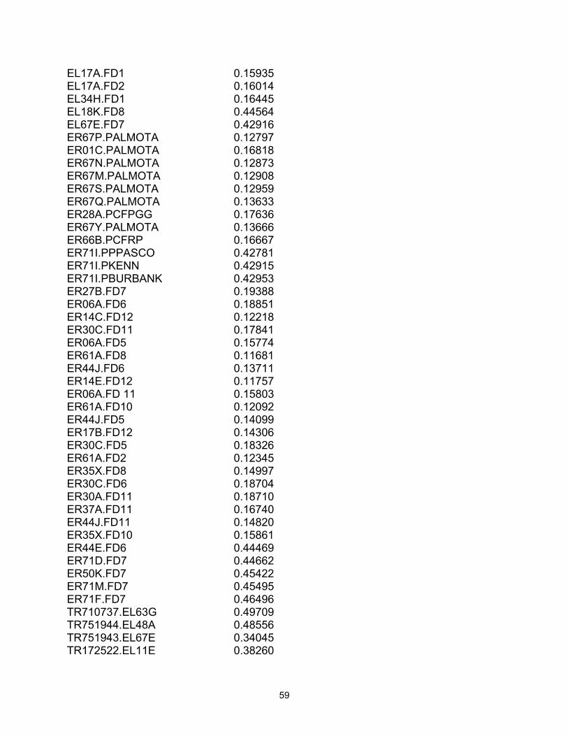
EL17A.FD1 0.15935 EL17A.FD2 0.16014 EL34H.FD1 0.16445 EL18K.FD8 0.44564 EL67E.FD7 0.42916 ER67P.PALMOTA 0.12797 ER01C.PALMOTA 0.16818 ER67N.PALMOTA 0.12873 ER67M.PALMOTA 0.12908 ER67S.PALMOTA 0.12959 ER67Q.PALMOTA 0.13633 ER28A.PCFPGG 0.17636 ER67Y.PALMOTA 0.13666 ER66B.PCFRP 0.16667 ER71I.PPPASCO 0.42781 ER71I.PKENN 0.42915 ER71I.PBURBANK 0.42953 ER27B.FD7 0.19388 ER06A.FD6 0.18851 ER14C.FD12 0.12218 ER30C.FD11 0.17841 ER06A.FD5 0.15774 ER61A.FD8 0.11681 ER44J.FD6 0.13711 ER14E.FD12 0.11757 ER06A.FD 11 0.15803 ER61A.FD10 0.12092 ER44J.FD5 0.14099 ER17B.FD12 0.14306 ER30C.FD5 0.18326 ER61A.FD2 0.12345 ER35X.FD8 0.14997 ER30C.FD6 0.18704 ER30A.FD11 0.18710 ER37A.FD11 0.16740 ER44J.FD11 0.14820 ER35X.FD10 0.15861 ER44E.FD6 0.44469 ER71D.FD7 0.44662 ER50K.FD7 0.45422 ER71M.FD7 0.45495 ER71F.FD7 0.46496 TR710737.EL63G 0.49709 TR751944.EL48A 0.48556 TR751943.EL67E 0.34045 TR172522.EL11E 0.38260

59

TR012033.EL351 0.32082 TR752042.EL25D 0.38857 TR751845.EL33X 0.40010 TR752042.EL50H 0.32222 TR751439.EL28J 0.35984 TR752042.EL50G 0.30604 TR231240.EL41M 0.26395 TR390311.EL17E 0.57591 TR390311.EL43D 0.59158 TR751545.ER67T 0.36125 TR771021.ER06A 0.36940 TR632643.ER71D 0.40694 TR252126.ER35X 0.38940 TR751944.ER33B 0.46299 TR432537.ER35U 0.32432 TR432537.ER16A 0.31324 TR072220.ER11X 0.25311 TR432336.ER35P 0.32039 TR011538.ER28G 0.25937 TR432539.ER46A 0.31586 TR632346.ER71J 0.34469 TR632540.ER46D 0.30864 TR751538.ER28G 0.24045 TR751544.ER67S 0.27412 TR011935.ER47A 0.25431 TR432538.ER16D 0.27255 TR751841.ER52J 0.27185 TR752043.ER50A 0.27184 TR390412.ER27B 0.51682 TR390312.ER27B 0.53241 TR751146.PWILMA 0.13678 TR751146.PCLARK 0.10805 TR231340.PCFPGG 0.10290 TR71073 I.PWALLULA 0.07877 TR231340.PCFRP 0.07493 TR71063 I.PPTKELLY 0.06682 TR231443.PALMOTA 0.06133 TR031145.PCLARK 0.05860 TR71073 I.PPTKELLY 0.05808 TR751440.PCFPGG 0.05794 TR031145.PWILMA 0.05776 TR390320.PROOSVLT 0.05762 TR751440.PCFRP 0.05748 TR390316.PBIGGS 0.05701 TR710631.PWALLULA 0.05683 TR653439.PWILMA 0.34677

60

TR513043.PKENN 0.34758 TR513043.PBURBANK 0.34797 TR653439.PLYONSF 0.34872 TR653439.PWINDUST 0.35179 TR771022.FD5 0.11233 TR771021.FD6 0.09661 TR251924.FD10 0.08950 TR251829.FD1 0.06855 TR251830.FD1 0.06717 TR770922.FD11 0.06705 TR710731.FD9 0.06252 TR252024.FD8 0.05954 TR251924.FD8 0.05948 TR770923.FD11 0.05853 TR771021.FD5 0.05810 TR251923.FD10 0.05808 TR632143.FD7 0.36051 TR632641.FD7 0.36195 TR751743.FD7 0.36242 TR751246.FD10 0.36402 TR632443.FD7 0.36418 TR632441.FD5 0.36583 TR632544.FD7 0.36619 TR6326-43.FD7 0.36630 TR751843.FD7 0.36781 TR632343.FD7 0.37206 TR632743.FD7 0.37481 TR632644.FD7 0.37861 TR632545.FD7 0.37915 TR632444.FD7 0.38049 TR632645.FD7 0.38226 PARAMETER WSUP(N) AVAILABLE WHEAT BU / TR011530 238605.0 TR011531 426408.0 TR011532 312468.0 TR011533 319029.0 TR011534 304851.0 TR011535 396002.0 TR011536 195014.0 TR011537 300501.0 TR011538 44093.0 TR011628 12390.0 TR011630 664014.0 TR771416 15140.0 TR771418 1090.0 /; PARAMETER BSUP(N) AVAILABLE BARLEY BU / TR011531 74981.0 TR011535 1066.0 TR011536 3305.0

61

TR011628 3632.0 TR011629 16347.0 TR011631 34838.0 TR011632 17316.0 TR771123 154.0 TR771217 1965.0 TR771220 531.0 TR771416 2694.0 TR771418 1773.0 /; PARAMETER RAILCAPW(N) RAIL CAPACITY FOR WHEAT ELEV W RAIL / ER00A 256000 ER00K 119700 ER02B 48000 ER09A 600000 ER09E 100000 ER09G 400000 ER091 100000 ER67C 20672 ER67Q 5476 ER67R 789232 ER71A 446500 ER71D 339150 ER71F 188100 ER711 716300 ER71J 157700 ER71M 324900 /; PARAMETER RAILCAPB(N) RAIL CAPACITY FOR BARLEY / ER02B 16000 ER02F 6400 ER16A 150000 ER16D 200000 ER18A 184933 ER18B 90048 ER20A 400 ER33B 51512 ER35A 71966 ER67M 6924 ER67P 96000 ER67R 322585 ER71A 336600 ER71D 256700 ER71F 142800 ER711 541450 ER71J 119850 ER71M 461550 /; PARAMETER CAPRHS(N) ELEV CAPACITIES / ER00A 2197000 ER00B 62000 EL00C 575000 EL00D 670000 ER68E 567000 ER71A 901000 ER71D 687000

62

ER71F 381000 EL71G 160000 ER711 1449000 ER71J 320000 ER71M 1235000 EL710 445000 /; PARAMETER BDEM(N) BARLEY DEMAND AT DEST SITES / PORTLAND 10414449 FD1 379473 FD2 43663 FD3 6238 FD4 0 FD5 4990095 FD6 1965 FD7 9356 FD8 124752 FD9 218317 FD10 18713 FD11 24950 FD12 486534/; PARAMETER CAPRHS2(N) UPDATED ELEV. CAPACITIES; CAPRHS2(N) = 1*CAPRHS(N); PARAMETER RAILCAPW2(N) UPDATED WHT RAIL MAX VALUES; PARAMETER RAILCAPB2(N) UPDATED BARLEY RAIL MAX VALUES; RAILCAPW2(N) = 1*RAILCAPW(N); RAILCAPB2(N) = 1*RAILCAPB(N); VARIABLES W(NNP,M) WHEAT FLOW ON ARCS N TO NP VIA MODE M B(N,NP,M) BARLEY FLOW ON ARCS N TO NP VIA MODE M TC TOTAL COST WTC TOTAL COST WHEAT BTC TOTAL COST BARLEY TRW TOTAL WHEAT RAIL TRB TOTAL BARLEY RAIL POSITIVE VARIABLES W, B; EQUATIONS WNB(N) NODE BALANCE WHEAT WDB(N) DESTINATION BALANCE WHEAT WSB(N) SUPPLY BALANCE WHEAT BNB(N) NODE BALANCE BARLEY BDB(N) DESTINATION BALANCE BARLEY BSB(N) SUPPLY BALANCE BARLEY CAP(N) CAPACITIES ON ELEVATORS RAILW(N) RAIL CAPACITY FOR WHEAT RAILB(N) RAIL CAPACITY FOR BARLEY T01 LIMIT ON ADAMS COUNTY TR TO PORT T05 LIMIT ON BENTON COUNTY TR TO PORT T07 LIMIT ON CHELAN COUNTY TR TO PORT T13 LIMIT ON COLUMBIA COUNTY TR TO PORT

63

T17 LIMIT ON DOUGLAS COUNTY TR TO PORT T21 LIMIT ON FRANKLIN COUNTY TR TO PORT T23 LIMIT ON GARFIELD COUNTY TR TO PORT T25 LIMIT ON GRANT COUNTY TR TO PORT T37 LIMIT ON KIMTAS COUNTY TR TO PORT T39 LIMIT ON KLICKITAT COUNTY TR TO PORT T43 LIMIT ON LINCOLN COUNTY TR TO PORT T47 LIMIT ON OKANOGAN COUNTY TR TO PORT T63 LIMIT ON SPOKANECOUNTY TR TO PORT T65 LIMIT ON STEVENS COUNTY TR TO PORT T71 LIMIT ON WALLA WALLA COUNTY TR TO PORT T75 LIMIT ON WHITMAN COUNTYFR TO PORT T77 LIMIT ON YAKIMA COUNTY TR TO PORT WCOST ACCTING: TOTAL COST WHEAT BCOST ACCTING. TOTAL COST BARLEY TCOST ACCTTNG: TOTAL COST; WDB(WD).. SUM((WINT,M)$WARCS(WINT,WD,M),W(WINT,WD,M))=G=132836124; WSB(WS 1).. SUM((WINT,M)$WARCS(WS1,WINT,M),W(WS1,WINT,M)) =L= WSUP(WS 1); WNB(WINT)SSLJM((N,M),WARCS(WINT,N,M)).. SUM((WS2,M)$WARCS(WS2,WINT,M), W(WS2,WINT,M)) =E= SUM((WD2,M)$WARCS(WINT,WD2,M), W(WINT,WD2,M)) T01.. SUM((C01,IPORT,M)SWARCS(C01,IPORT,M),W(C01,IPORT,M)) =L=4469867; T05.. SUM((C05,IPORT,M)SWARCS(C05,IPORT,M),W(C05,IPORT,M)) =L=5089365; T07.. SUM((C07,IPORT,M)SWARCS(C07,IPORT,M),W(C07,IPORT,M)) =L=14300; T13.. SUM((C13,IPORT,M)SWARCS(C13,IPORT,M),W(C13,IPORT,M)) =L=867058; T17.. SUM((C17,IPORT,M)SWARCS(C17,IPORT,M),W(C17,IPORT,M)) =L=5881930; T21.. SUM((C21,IPORT,M)$WARCS(C21,IPORT,M),W(C21,IPORT,M)) =L=4703398; T23.. SUM((C23,IPORT,M)SWARCS(C23,IPORT,M),W(C23,IPORT,M)) =L=3800669;

64

T25.. SUM((C25,IPORT,M)SWARCS(C25,IPORT,M),W(C25,IPORT,M)) =L=4642981; T37.. SUM((C37,IPORT,M)SWARCS(C37,IPORT,M),W(C37,IPORT,M)) =L=141519; T39.. SUM((C39,IPORT,M)$WARCS(C39,IPORT,M),W(C39,IPORT,M)) =L=2242982; T43.. SUM((C43,IPORT,M)SWARCS(C43,IPORT,M),W(C43,IPORT,M)) =L=7680181; T47.. SUM((C47,IPORT,M)SWARCS(C47,IPORT,M),W(C47,IPORT,M)) =L=121171; T63.. SUM((C63,IPORT,M)SWARCS(C63,IPORT,M),W(C63,IPORT,M)) =L=577097; T65.. SUM((C65,IPORT,M)SWARCS(C65,IPORT,M),W(C65,IPORT,M)) =L=289432; T71.. SUM((C71,IPORT,M)$WARCS(C71,IPORT,M),W(C71,IPORT,M)) =L=1795242; T75.. SUM((C75,IPORT,M)$WARCS(C75,IPORT,M),W(C75,IPORT,M)) =L=11530216; T77.. SUM((C77,IPORT,M)SWARCS(C77,IPORT,M),W(C77,IPORT,M)) =L=995879; BDB(BD).. SUM((BS2,M)$BARCS(BS2,BD,M),B(BS2,BD,M))=G=BDEM(BD); BSB(BS1).. SUM((BINT2,M)$BARCS(BS1,BINT2,M),B(BS1,BINT2,M)) =L= BSUP(BS1); BNB(BINT)$SUM((N,M),BARCS(BINT,N,M)).. SUM((BS2,M)$BARCS(BS2,BINT,M), B(BS2,BINT,M)) =E= SUM((BD2,M)$BARCS(BINT,BD2,M), B(BINT,BD2,M)); CAP(CAPSET).. SUM((WS2,M)SWARCS(WS2,CAPSET,M), W(WS2,CAPSET,M)) + SUM((BS2,M)SBARCS(BS2,CAPSET,M), B(BS2,CAPSET,M)) =L= CAPRHS2(CAPSET);

65

RAILW(WINT).. SUM((WD,R)$WARCS(WINT,WD,R), W(WINT,WD,R)) =L= RAILCAPW(WINT); RAILB(BINT).. SUM((BD,R)$BARCS(BINT,BD,R), B(BINT,BD,R)) =L= RAILCAPB(BINT); TCOST.. TC=E=SUM((N,NP,M)$WARCS(N,NP,M),WARCS(N,NP,M)*W(N,NP,M))+ SUM((N,NP,M)$BARCS(N,NP,M),BARCS(N,NP,M)*B(N,NP,M)) ; WCOST.. WTC=E=SUM((N,NP,M)$WARCS(N,NP,M),WARCS(NNP,M)*W(N,NP,M)); BCOST.. BTC=E=SUM((N,NP,M)$BARCS(NNP,M),BARCS(N,NP,M)*B(N,NP,M)); MODEL TEST /ALL/; OPTION LIMROW = 5; OPTION LIMCOL = 5; OPTION RESLIM = 5000; OPTION ITERLIM = 100000; SOLVE TEST MINIMIZING TC USING LP; DISPLAY W.L, B.L; FILE RES /’EJ.DAT’/; PUT RES; PUT "TOTAL COST = /; PUT TC.L /; PUT /; PUT "TOTAL COST WHEAT = /; PUT WTC.L /; PUT /; PUT 'TOTAIL COST BARLEY =" /; PUT BTC.L /; PUT /; ***PUT "WHEAT ARCS" /; ***LOOP ((N,NP,M), ***IF (W(N,NP,M) GT 0, ***PUT N.TL, NP.TL, M.TL, W.L(N,NP,M) /)); PUT "WHEAT ARCS FOR TRS TO ELEVATORS" /; LOOP ((WS1,CAPSET,M), IF (W(WS1,CAPSET,M) GT 0, PUT WS 1.TL, CAPSET.TL, M.TL, W.L(WS1,CAPSET,M) /)); PUT "WHEAT ARCS FOR TRS TO RIVER PORTS” /; LOOP ((WS1,IPORT,M), IF (W(WS1,IPORT,M) GT 0 PUT WS1.TL, IPORT.TL, M.TL, W.L(WS1,IPORT,M) /));

66

PUT “WHEAT ARCS FOR ELEVATORS TO ELEVATORS WITH RAIL” /; LOOP ((ELEV,RELEV,M), IF (W(ELEV,RELEV,M) GT 0, PUT ELEV.TL, RELEV.TL, M.TL, W.L(ELEV,RELEV,M) /)); PUT “WHEAT ARCS FOR ELEVATORS TO RIVER PORTS” /; LOOP ((CAPSET,IPORT,M), IF (W(CAPSET,IPORT,M) GT 0, PUT CAPSET.TL, IPORT.TL, M.TL, W.L(CAPSET,IPORT,M) /)); PUT “WHEAT ARCS FOR RIVER PORTS TO PORTLAND” /; LOOP ((IPORT,WD,M), IF (W(IPORT,WD,M) GT 0, PUT IPORT.TL, WD.TL, M.TL, W.L(IPORT,WD,M) /)); PUT “WHEAT ARCS FOR ELEVATORS WITH RAIL TO PORTLAND” /; LOOP (RELEV,WD,M), IF (W(RELEV,WD,M) GT 0, PUT RELEV.TL, WD.TL, M.TL, W.L(RELEV,WD,M) /)); ***PUT “BARLEY ARCS” /; ***LOOP ((N,NP,M), ***IF (B(N,NP,M) GT 0, ***PUT N.TL, NP.TL, M.TL, B.L(N,NP,M) /)); PUT “BARLEY ARCS FOR TRS TO ELEVATORS” /; LOOP ((BS1,CAPSET,M), IF (B(BS1,CAPSET,M) GT 0 PUT BS1.TL, CAPTSET.TL, M.TL, B.L(BS1,CAPSET,M) /)); PUT “BARLEY ARCS FOR TRS TO RIVER PORTS” /; LOOP ((BS1,IPORT,M), IF (B(BS1,IPORT,M) GT 0, PUT BS1.TL, IPORT.TL, M.TL, B.L(BS1,IPORT,M) /)); PUT “BARLEY ARCS FOR ELEVATORS TO ELEVATORS WITH RAIL” /; LOOP ((ELEV,RELEV,M), IF (B(ELEV,RELEV,M) GT 0, PUT ELEV.TL, RELEV.TL, M.TL, B.L(ELEV,RELEV,M) /)); PUT “BARLEY ARCS FOR ELEVATORS TO RIVER PORTS” /; LOOP ((CAPSET,IPORT,M), IF (B(CAPSET,IPORT,M) GT 0, PUT CAPSET.TL, IPORT.TL, M.TL, B.L(CAPSET,IPORT,M) /));

67

68

PUT “BARLEY ARCS FOR RIVER PORTS TO PORTLAND” /; LOOP ((IPORT,BD,M), IF (B(IPORT,BD,M) GT 0, PUT IPORT.TL, BD.TL, M.TL, B.L(IPORT,BD,M) /)); PUT "BARLEY ARCS FOR ELEVATORS WITH RAIL TO PORTLAND” /; LOOP ((RELEV,BD,M), IF (B(RELEV,BD,M) GT 0, PUT RELEV.TL, BD.TL, M.TL, B.L(RELEV,BD,M) /)); PUT "BARLEY ARCS FOR TRS TO FEEDLOTS" /; LOOP ((BS1,BFD,M), IF (B(BS1,BFD,M) GT 0, PUT BS1.TL, BFD.TL, M.TL, B.L(BS1,BFD,M) /)); PUT "BARLEY ARCS FOR ELEVATORS TO FEEDLOTS" /; LOOP ((CAPSET,BFD,M), IF (B(CAPSET,BFD,M) GT 0, PUT CAPSET.TL, BFD.TL, M.TL, B.L(CAPSET,BFD,M) /)); ***PUT "DUAL PRICES FOR ELEVATOR CAPACITY “ /; ***LOOP ((CAPSET), ***PUT CAPSET.TL, CAP.M(CAPSET) /); ***PUT "DUAL PRICES FOR WHEAT RAIL " /; ***LOOP ((WINT), ***PUT WINT.TL, RAILW.M(WINT) /); ***PUT “DUAL PRICES FOR BARLEY RAIL” /; ***LOOP ((BINT), ***PUT BINT.TL, RAILB.M(BINT) /);