a global macroeconomic forecasting model for the philippines ruperto majuca, ph.d (illinois), j.d....

A Global MacroeconomicForecasting Model for the Philippines

Ruperto Majuca, Ph.D (Illinois), J.D.

De La Salle University, Manila

51st Philippine Economic Society Annual MeetingNovember 2013 (Makati City, Philippines)

Outline

Introduction The Model’s Stochastic Equations Estimation Methods Estimation Results Summary of Findings and Conclusions

Table of Contents

Introduction The Model’s Stochastic Equations Estimation Methods Estimation Results Summary of Findings and Conclusions

Motivating Questions How does a slowdown in U.S. or a U.S. debt

default affect PH economy, directly & indirectly via effects on EU, China, Japan, ASEAN?

■ How does a debt crisis in EU, or China slowdown, affect U.S., China, Japan, ASEAN, and PH directly & indirectly?

■ What has greater impact on PH, shocks from the U.S., EU, China, Japan, ASEAN, or its own shocks?

■ What are the ripple effects of the shocks to Philippine GDP, unemployment, inflation, interest rates, exchange rates, etc.?

Research Interests

Economic & financial linkages PH with ASEAN, U.S., EU, China, Japan, & those economies’ linkages with each other

■ Transmission of shocks from U.S., E.U., Japan, and China to ASEAN, & PH

■ Quantifying the ripple effects to ASEAN & AMSs’ GDP growth, inflation, interest rates, exchange rate, & unemployment

■ Implications for policy and macroeconomic management

Research Methodology, 1 Traditional PH models (equation-by-equation OLS,

ECM)NEDA QMMPIDSAteneo (AMFM), others

Simultaneity bias, exogeneity issueEstimates are biased and inconsistentIncreasing sample cannot cure bias in estimates

Lucas (1976) critiqueCoefficient estimates are not policy invariantLucas: conclusions and policy advice based on

these models are invalid and misleading

Research Methodology, 2 Post Lucas critique. Now standard: modern,

dynamic quantitative economics Dynamic stochastic general equilibrium (DSGE

models)Global projection models

Utilizes state of the art: Bayesian methods This work: global projection model to analyze

interplay of key macroeconomic variables across countries/regionsU.S., E.U., Japan, China, ASEAN, PHGDP growth, inflation, interest rates, exchange rate,

unemployment

Designed to capture cross-regions and cross-country macroeconomic linkages (e.g., US, EU, Japan, China, ASEAN, AMS)

Traces cross-border ripple effects of key macroeconomic variables (GDP growth, inflation, interest rates, exchange rates, unemployment)

Bayesian estimation techniquesPriors plus Bayesian updating via Kalman filter;

Markov Chain Monte Carlo

The Global Projection Model

Table of Contents

Introduction

The Model’s Stochastic Equations Estimation Methods Estimation Results Summary of Findings and Conclusions

Potential Output

NAIRU

Equilibrium Real Interest Rate

GPM Stochastic Equations, 1

𝑟𝑖,𝑡 = 𝑅𝑖,𝑡 − 𝑅𝑖,𝑡

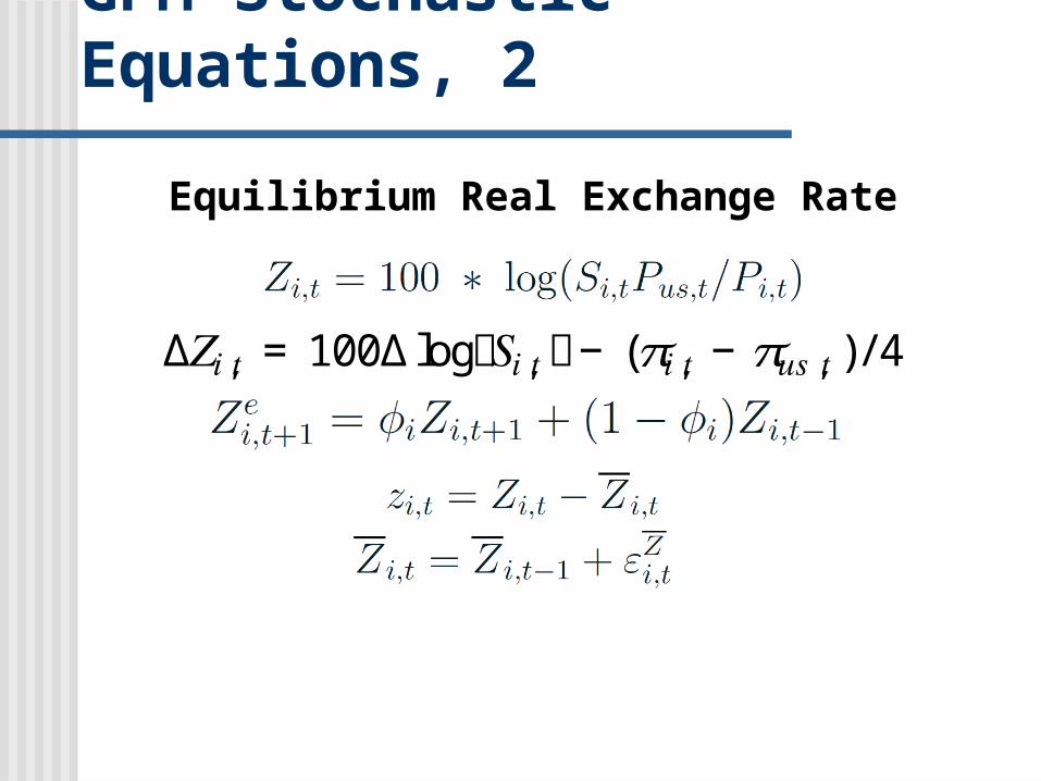
Equilibrium Real Exchange Rate


Δ𝑍𝑖,𝑡 = 100Δlog൫𝑆𝑖,𝑡൯− (𝜋𝑖,𝑡 − 𝜋𝑢𝑠,𝑡)/4

Output Gap (Aggregate Demand / IS Curve)

Inflation (New Keynesian Phillips Curve)


Policy Interest Rate (Taylor Type Rule)

Uncovered Interest Parity (Bilateral Real Exchange Rate)

Unemployment Rate



Equations Incorporating BLT_US

Table of Contents

Introduction The Model’s Stochastic Equations

Estimation Methods Estimation Results Summary of Findings and Conclusions

Bayesian Estimation

Mixture between classical estimation and calibration of macro models

Puts some weight on the priors and some weight on the data

Combine prior and MLE estimation via Kalman filter

Recover posterior distribution via MCMC (Metropolis Hastings)

Estimation Strategy

Start with GPM4 (US, EU, Japan, China); estimate coefficients

■ Proceed with GPM5 (US, EU, Japan, China + ASEAN), fixing coefficient for GPM4. Assumes ASEAN doesn’t change GPM4 coefficients

■ Then proceed with GPM6 (US, EU, Japan, China, ASEAN + Philippines), mutatis mutandis

■ 250,000 MH draws each stage; first 30% used as burn-in

Data Requirements

Consumer price index Real gross domestic product Nominal interest rate Nominal exchange rate Unemployment rate Bank lending variable for US CPI, GDP and ER are in logs

Table of Contents

Introduction The Model’s Stochastic Equations Estimation Methods

Estimation Results Summary of Findings and Conclusions

Estimation Results: GPM5 Parameters

Prior distribution

Prior mean

Prior s.d. Posterior mode

s.d.

alpha1_AS beta 0.750 0.1000 0.8221 0.0356 alpha2_AS gamm 0.100 0.0500 0.0687 0.0160 alpha3_AS beta 0.500 0.2000 0.4512 0.0548 beta1_AS gamm 0.650 0.1000 0.6353 0.0247 beta2_AS beta 0.150 0.1000 0.0943 0.0320 beta3_AS gamm 0.150 0.1000 0.0690 0.0126 gamma1_AS beta 0.750 0.1000 0.9430 0.0155 gamma2_AS gamm 1.100 0.1000 1.0857 0.0346 gamma4_AS gamm 0.500 0.2000 0.4719 0.0576 lambda1_AS beta 0.500 0.1000 0.6299 0.0296 lambda2_AS gamm 0.400 0.1000 0.3774 0.0198 lambda3_AS gamm 0.050 0.0100 0.0480 0.0032 rho_AS beta 0.500 0.2000 0.0110 0.0689 phi_AS beta 0.600 0.1000 0.6625 0.0258 tau_AS beta 0.050 0.0200 0.0427 0.0049 rr_bar_AS_ss norm 1.500 0.1000 1.4835 0.0494 growth_AS_ss norm 5.000 0.2000 5.0157 0.0651 beta_reergap_AS gamm 0.050 0.0200 0.0472 0.0074

Prior

distribution Prior mean

Prior s.d.

Posterior mode

s.d.

RES_PIE_AS invg 3.000 Inf 3.6982 0.4221

RES_Y_AS invg 0.500 1.0000 0.2406 0.1084

RES_RS_AS invg 0.600 1.0000 0.2213 0.0347

RES_LGDP_BAR_AS invg 0.200 Inf 18.5265 0.9173

RES_G_AS invg 0.100 Inf 0.0460 0.0381

RES_RR_BAR_AS invg 0.200 Inf 0.1877 0.5291

RES_UNR_GAP_AS invg 0.600 1.0000 0.2488 0.0478

RES_UNR_BAR_AS invg 0.100 Inf 0.0461 0.0493

RES_UNR_G_AS invg 0.100 Inf 0.0472 0.0237

RES_LZ_BAR_AS invg 5.000 Inf 4.8714 0.8198

RES_RR_DIFF_AS invg 1.000 Inf 0.4591 0.3230

Estimation Results: GPM5 S.D. of Structural Shocks

Estimation Results: GPM6 Parameters, 1

Prior distribution

Prior mean

Prior s.d. Posterior mode

s.d.

alpha1_PH beta 0.750 0.0500 0.7810 0.0434

alpha2_PH gamm 0.100 0.0500 0.0882 0.0503

alpha3_PH beta 0.500 0.2000 0.4673 0.3086

beta_fact_PH gamm 0.150 0.1000 0.1171 0.1024

beta1_PH gamm 0.650 0.1000 0.5710 0.0806

beta2_PH beta 0.150 0.0500 0.1234 0.0446

beta3_PH gamm 0.150 0.0200 0.1310 0.0181

gamma1_PH beta 0.900 0.0500 0.9101 0.0207

gamma2_PH gamm 1.100 0.5000 0.8872 0.3600

gamma4_PH gamm 0.500 0.2000 0.4034 0.1745

growth_PH_ss norm 5.000 0.2000 5.0000 0.2000

lambda1_PH beta 0.500 0.0500 0.5616 0.0477

lambda2_PH gamm 0.400 0.1000 0.3522 0.0876

lambda3_PH gamm 0.050 0.0300 0.0390 0.0292

lambda1_RS_PH beta 0.500 0.1000 0.4469 0.0868

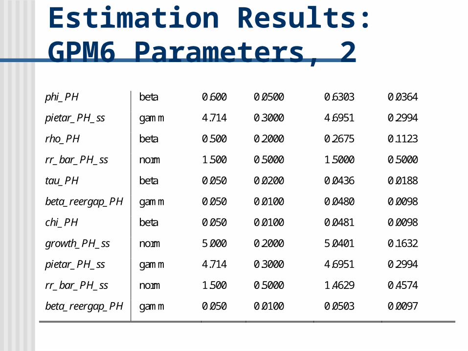
Estimation Results: GPM6 Parameters, 2phi_PH beta 0.600 0.0500 0.6303 0.0364

pietar_PH_ss gamm 4.714 0.3000 4.6951 0.2994

rho_PH beta 0.500 0.2000 0.2675 0.1123

rr_bar_PH_ss norm 1.500 0.5000 1.5000 0.5000

tau_PH beta 0.050 0.0200 0.0436 0.0188

beta_reergap_PH gamm 0.050 0.0100 0.0480 0.0098

chi_PH beta 0.050 0.0100 0.0481 0.0098

growth_PH_ss norm 5.000 0.2000 5.0401 0.1632

pietar_PH_ss gamm 4.714 0.3000 4.6951 0.2994

rr_bar_PH_ss norm 1.500 0.5000 1.4629 0.4574

beta_reergap_PH gamm 0.050 0.0100 0.0503 0.0097

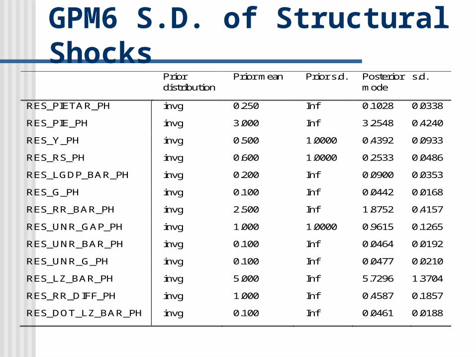
Estimation Results: GPM6 S.D. of Structural Shocks

Prior distribution

Prior mean Prior s.d. Posterior mode

s.d.

RES_PIETAR_PH invg 0.250 Inf 0.1028 0.0338

RES_PIE_PH invg 3.000 Inf 3.2548 0.4240

RES_Y_PH invg 0.500 1.0000 0.4392 0.0933

RES_RS_PH invg 0.600 1.0000 0.2533 0.0486

RES_LGDP_BAR_PH invg 0.200 Inf 0.0900 0.0353

RES_G_PH invg 0.100 Inf 0.0442 0.0168

RES_RR_BAR_PH invg 2.500 Inf 1.8752 0.4157

RES_UNR_GAP_PH invg 1.000 1.0000 0.9615 0.1265

RES_UNR_BAR_PH invg 0.100 Inf 0.0464 0.0192

RES_UNR_G_PH invg 0.100 Inf 0.0477 0.0210

RES_LZ_BAR_PH invg 5.000 Inf 5.7296 1.3704

RES_RR_DIFF_PH invg 1.000 Inf 0.4587 0.1857

RES_DOT_LZ_BAR_PH invg 0.100 Inf 0.0461 0.0188

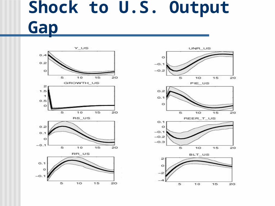
Impulse Responses:Shock to U.S. Output Gap

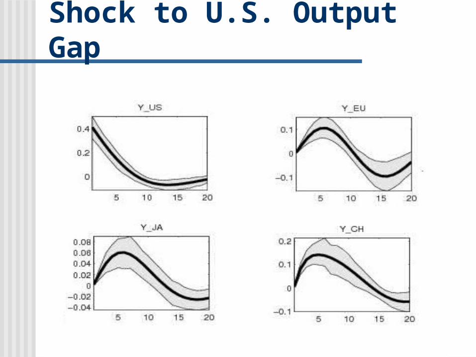
Impulse Responses:Shock to Euro Area Output Gap

Impulse Responses:Shock to Japan Output Gap

Impulse Responses:Shock to China Output Gap

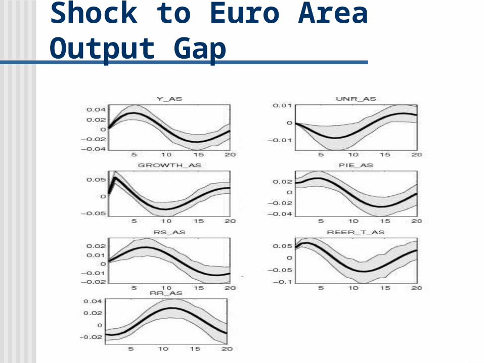
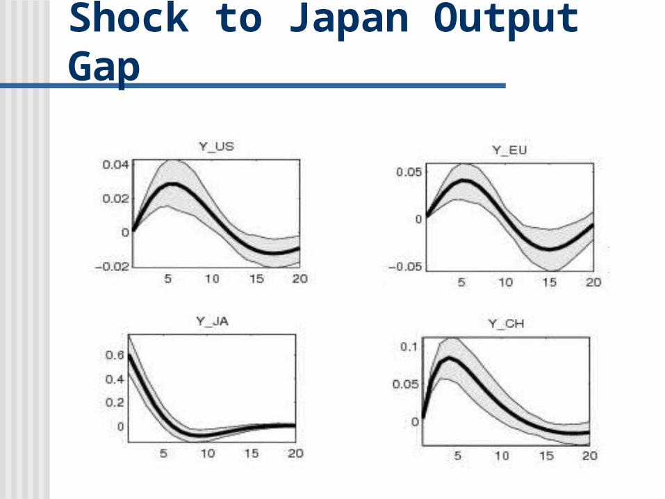
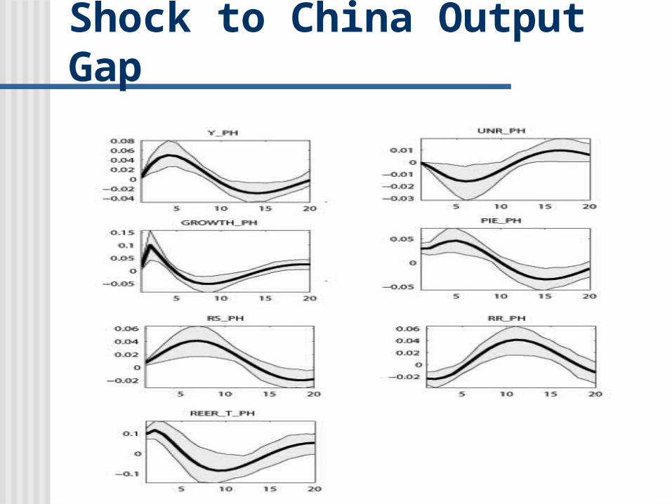
Impulse Responses:Shock to Japan Output Gap

Impulse Responses:Shock to China Output Gap

Impulse Responses:Shock to ASEAN Output Gap

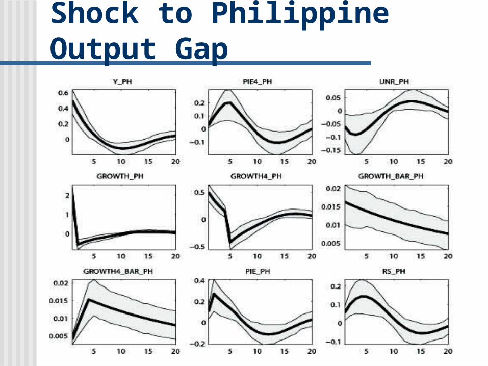
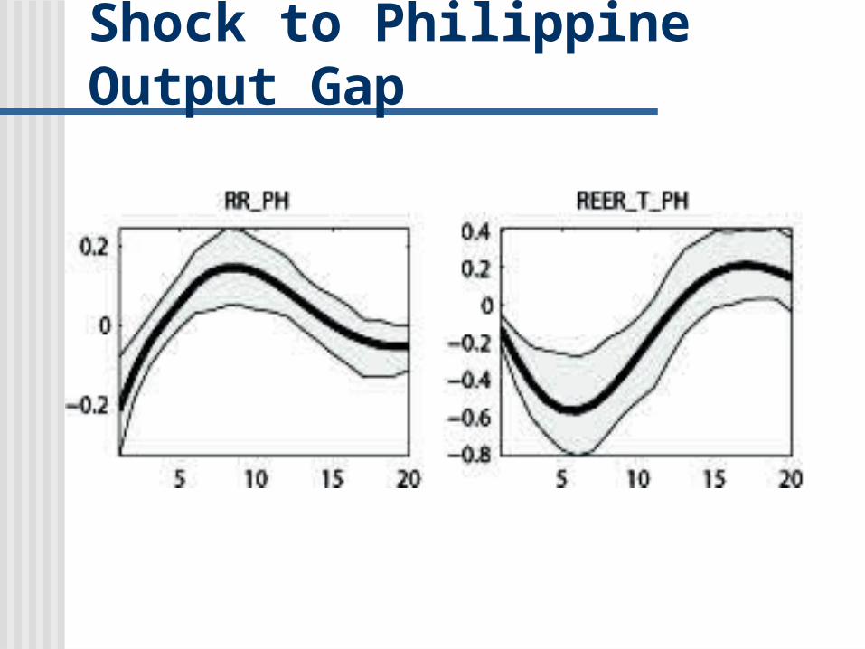
Impulse Responses:Shock to Philippine Output Gap

Table of Contents

Introduction The Model’s Stochastic Equations Estimation Methods Estimation Results

Summary of Findings and Conclusions

Findings and Conclusions, 1 Existing PH models (NEDA QMM, PIDS, AMFM,

etc.) using equation-by-equation OLS, ECM)Simultaneity bias/inconsistency issueLucas (1976): coefficients not policy invariant;

conclusions & policy advice are invalid and misleading

Now standard: modern, dynamic quantitative economics (utilizing Bayesian methods)Dynamic stochastic general equilibrium (DSGE

models)Global projection models

Findings and Conclusions, 2

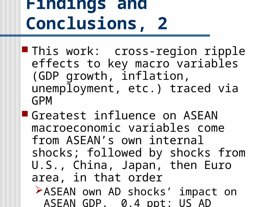
This work: cross-region ripple effects to key macro variables (GDP growth, inflation, unemployment, etc.) traced via GPM

Greatest influence on ASEAN macroeconomic variables come from ASEAN’s own internal shocks; followed by shocks from U.S., China, Japan, then Euro area, in that orderASEAN own AD shocks’ impact on ASEAN

GDP, 0.4 ppt; US AD impact (peaks after 5 or 6 quarters), about 1/7 of ASEAN impact; China AD shock, about 1/9 ASEAN’s; Japan, 1/10; EU, 1/11

Findings and Conclusions, 3 For AMS like PH, domestic shocks also capture

much of the influence on own macroeconomic variables. In the case of PH, this is followed by shocks from the U.S., Japan and China, then ASEAN and Euro area.PH AD shock’s impact to PH GDP, about 0.5

percent; US shock’s impact (peaks after about 5 or 6 quarters), about 1/7 of PH shock’s impact; Japan and China, about 1/10; ASEAN and EU, about 1/17.

Findings and Conclusions, 4

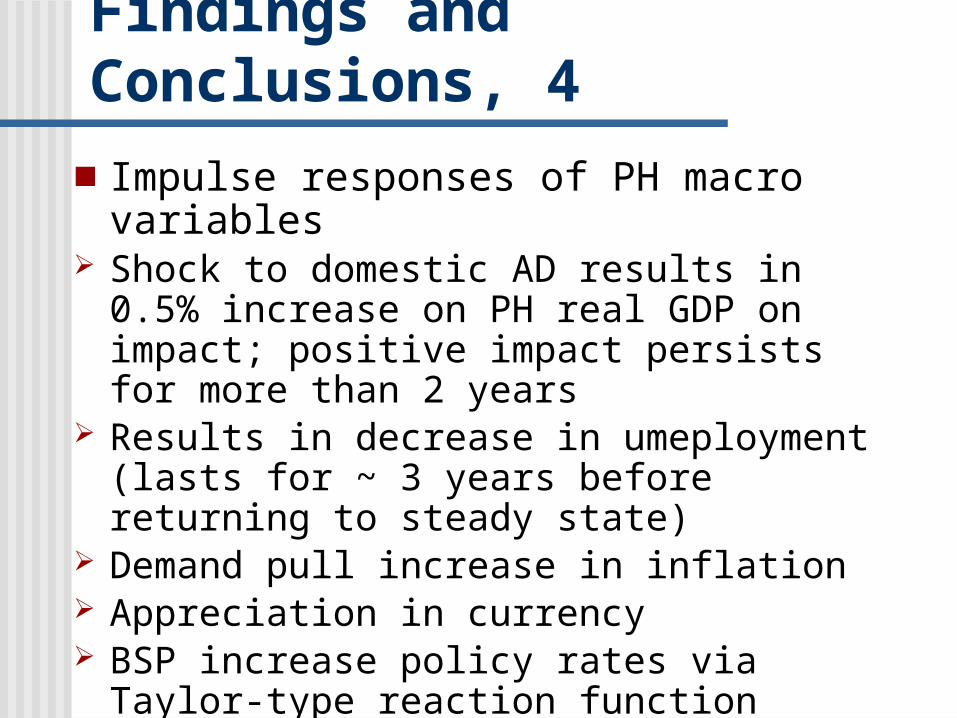
■ Impulse responses of PH macro variables Shock to domestic AD results in 0.5% increase on

PH real GDP on impact; positive impact persists for more than 2 years

Results in decrease in umeployment (lasts for ~ 3 years before returning to steady state)

Demand pull increase in inflation Appreciation in currency BSP increase policy rates via Taylor-type reaction

function

Thank You!

a global macroeconomic forecasting model for the philippines ruperto majuca, ph.d (illinois), j.d....

Documents

unemployment slide

philippines slide

misleading slide

macroeconomic management

exchange rates

global projection model

ph gdp growth

china slowdown