a gradient-based approach for computing nash equilibria of

A GRADIENT-BASED APPROACH FOR COMPUTING NASH EQUILIBRIA OFLARGE SEQUENTIAL GAMES

SAMID HODA∗, ANDREW GILPIN†, AND JAVIER PENA∗

Abstract. We propose a new gradient based scheme to approximate Nash equilibria of large sequen-tial two-player, zero-sum games. The algorithm uses modern smoothing techniques for saddle-point

problems tailored specifically for the polytopes used in the Nash equilibrium problem.

1. Introduction

Equilibrium problems have long attracted the interest of game theorists and optimizers. The Nashequilibrium problem for two-player zero-sum sequential games can be modeled using linear program-ming [12]. In principle, these linear programs can be solved using any state-of-the-art linear program-ming solver (see Section 2). However, for most interesting games, the size of the game tree and thecorresponding linear program is enormous.

This problem seems to be particularly challenging from an optimization perspective. The polytope inthe linear programming formulation tends to be highly degenerate. This is one of the reasons active-setmethods seem to perform poorly on this class of problems [2]. Interior-point methods, despite theirgreat iteration complexity do not fare any better; they pay an enormous per iteration price arising fromthe matrix factorizations required at each iteration. For the size of games we are interested in solving, itis unlikely that an interior-point method will be able to complete even a single iteration in a reasonableamount of time.

Our approach sidesteps these difficulties by solving the basic saddle-point version of the problemusing a smoothing technique proposed by Nesterov [7, 8]. The smoothing step involves perturbing thesaddle point problem in order to transform it into a minimization problem of a convex function withLipschitz gradient. The latter problem in turn is amenable to an efficient gradient-based method. Thismethod has minimal memory requirements and a cost per iteration that is linear in the size of the gametree. In Section 3 we provide a summary of Nesterov’s recent results [7, 8].

At the heart of our approach is the construction of a family of prox functions for the polytopes arisingin the saddle-point formulation of zero-sum two-player sequential games. These prox functions providethe perturbation used in the smoothing portion of the algorithm. Moreover, the performance of thealgorithm depends entirely on finding appropriate prox functions for the constraint set of the problem.In Section 4 we present an inductive construction of nice prox functions for sequential games based on aparticular “lifting” operation used in convex analysis. The lifting operation produces a simple recursioninvolving subproblems over much simpler sets.

We conclude by considering games with a particular uniform structure. For these games we provethat the number of iterations required for obtaining an ε-solution is O(T 2/ε) where T is sublinear in thesize of the game tree.1

Date: July 6, 2007.* Tepper School of Business, Carnegie Mellon University.

† School of Computer Science, Carnegie Mellon University.1Since the solutions we compute have a duality gap of ε, we are actually computing ε-Nash equilibria in which each

player’s incentive to deviate from the strategy is at most ε. In fact, our solutions are ε-minimax solutions since each

player’s payoff guarantee does not depend on the opponent playing any particular strategy.

1

2 SAMID HODA∗, ANDREW GILPIN†, AND JAVIER PENA∗

1

I I

ii

II

A B C D

a ab b

root

2 -2

1

c d

E F1

-2

6 -6

1 -2 4 -2

G H G H

212

1 2

1

2

34

13

23

1 1

2 2 2

1 1 1

Figure 1. A graphical depiction of a two-player sequential game. The dotted linesenclose decision nodes in the same information set. The labels on the decision nodesindicate which player is making the decision while the labels on the edges indicate thechoices. Chance nodes are unlabeled and the edges are labeled with the probability ofeach chance move occurring.

2. Sequential games

In this section we review sequential games. In particular, we describe the sequence form of a gameand the resulting linear programming formulation [12], focusing on the realization polytope that arisesfrom this formulation.

2.1. Preliminaries. A finite sequential game is represented as an extensive form game [9]. The rootof the tree represents the starting point of the game while the leaves represent the termination points.The remaining internal nodes are the decision nodes; they indicate points in the game where one of theplayers (possibly the chance player) has to make a choice. The edges of the game tree are oriented fromthe root towards the leaves. Each edge leaving a particular decision node is labeled with the player’schoice.

A game tree may contain decision nodes that model random events in the game. It is customaryto associate these nodes with a fictitious chance player. The choices available to the chance player arecalled chance moves, which allow the modeling of situations in which the next branch of the game treeis reached randomly according to the probabilities dictated by the game.

The decision nodes are partitioned into information sets [5, 9]. Each information set is associatedwith exactly one player; moreover, the player has exactly the same set of choices at every decision nodein an information set. We assume, without loss of generality, that the choices at distinct informationsets are distinct. If u is an information set then Cu denotes the set of choices at u.

Example 1. Figure 1 illustrates a sequential game with two players. The information sets belongingto the first player are I1, . . . , I4 and the information sets belonging to the second player are i1 and i2.Observe that nodes belonging to the same information set have the same set of choices and that theset of choices corresponding to distinct information sets are disjoint. For example, Ci1 = {a, b} andCi2 = {c, d}. �

2.2. Sequence form. The sequence form of a game leads to a concise representation of strategies. Fortwo-player zero-sum games, this representation yields a concise linear programming formulation [3, 10,

A GRADIENT-BASED APPROACH FOR COMPUTING NASH EQUILIBRIA 3

11, 12].2 Each node in the game tree determines a unique sequence of choices from the root to thatnode for each of the players. A sequence for a player is represented by a string consisting of the labelson the edges corresponding to the choices made by the player and in the order the choices were made.The number of sequences is thus bounded by the number of nodes in the game tree.

Let U and S be the set of all information sets and the set of all sequences belonging to one of theplayers. The empty sequence ε is the sequence in which the player has not yet made a choice. Letσ : U → S be the function that maps each information set u ∈ U to the sequence of choices made bythe player to reach u. We denote the image σ(u) by σu. The set of all sequences S associated with theplayer can be expressed as

S := {ε} ∪ {σuc : u ∈ U, c ∈ Cu}.Note that σ is not necessarily one-to-one since many information sets may be reached by the samesequence of choices by the player. Two different information sets are parallel if they both belong to thesame player and are preceded by the same sequence of choices by that player, i.e. the information setsu and v ∈ U are parallel if σu = σv.

Example 2. The set of all information sets belonging to the first and second player in Figure 1 are

U1 = {I1, I2, I3, I4} and U2 = {i1, i2}.The set of all sequences for the first and second player are

S1 = {ε,A,B,C,D,BE,BF,CG,CH} and S2 = {ε, a, b, c, d}.The sequence of choices made by the first player to reach the information set I1 is σI1 = ε while to reachinformation set I3, the sequence is σI3 = B. Note that concatenating B to the empty sequence resultsin the string B. The string BF corresponds to the sequence in which the first player makes the choiceB followed by the choice F . This sequence does not lead to another information set for the first playerbut to one of two terminal nodes (leaves) determined by a chance move after the first player chooses F .

Observe that σI1 = σI2 = ε and both information sets belong to the first player; thus I1 and I2 areparallel information sets. Finally observe that I3 succeeds I1 while I4 succeeds I2 and σI3 = B 6= C =σI4 . �

A realization plan for the player is any vector x ∈ RS+ such that

(1) x(ε) = 1 and x(σu) =∑

c∈Cu

x(σuc) for all u ∈ U.

The complex (or realization polytope) associated with a player is the set of realization plans for thatplayer. Realization plans induce reduced behavioral strategies which specify a probability distributionover choices at all information sets except those for which a previous choice in the path to the root hasprobability zero. The complex is the convex hull of realization plans that induce deterministic reducedbehavioral strategies [12]. Furthermore, the extreme points of the complex are 0-1 vectors. There areexactly 1+ |U | equations defining the complex for the player. This system of equations has a coefficientmatrix of dimension (1 + |U |) × |S| with entries −1, 0 and 1. The vector on the right-hand side is allzeros except for the first entry which is equal to one.

Example 3. Continuing with the game shown in Figure 1, the complex corresponding to the first playeris Q1 := {x ∈ RS1

+ : Ex = e}, where

ε A B C D BE BF CG CH

E =

rootI1I2I3I4

1

−1 1 1−1 1 1

−1 1 1−1 1 1

, e =

10000

rootI1I2I3I4

.

2The sequence form representation requires that the players have perfect recall ; this means that all the decision nodesin a player’s information set are preceded by the same sequence of moves by that player. We assume that perfect recall

holds in all the results that follow.


The missing entries in the coefficient matrix are zero. Similarly, the complex corresponding to the secondplayer is Q2 := {y ∈ RS2

+ : Fy = f}, where

ε a b c d

F =rooti1i2

1−1 1 1−1 1 1

, f =

100

rooti1i2

.

�

Let S1 and S2 be the set of all sequences for the first and second player respectively. Then the payoffsat the leaves for the first player can be represented by a matrix in RS1×S2 , that is, a matrix whose rowsare indexed by the sequences in S1 and whose columns are indexed by the sequences in S2. Each playerhas their own payoff matrix and in the case of zero-sum games the payoff matrices are negatives of oneanother.

Consider a pair of sequences (s, t) ∈ S1 × S2. Suppose that the pair (s, t) leads to a leaf. Then the(s, t)-entry in the matrix is the sum, over all the leaves reachable by the pair of sequences (s, t), of thepayoff at each leaf multiplied by the probability of chance moves (if any) leading to that leaf. Otherwise,if the pair of sequences (s, t) do not lead to a leaf then the (s, t)-entry in the payoff matrix is zero.

Example 4. The payoff matrix for the first player in the game shown in Figure 1 is

ε a b c d

A =

εABCDBEBFCGCH

1 −11/2

1/2−1−1

1/2 2−1 −1

.

For example, to calculate the (B, a)-entry in the matrix we look at all leaves with the sequence (B, a).Since there is a single leaf with this sequence, we multiply the payoff at that leaf by any chance movesalong the path to the leaf. The payoff is 1 with a single chance move that occurs with probability 1/2;thus the (B, a)-entry is 1/2.

Observe that there are two leaves corresponding to the sequences (BF, b). Thus the (BF, b)-entry inthe matrix is the sum of the payoffs at both leaves multiplied by the probability of the chance movesalong the paths leading to the leaves. The calculation for the (BF, b)-entry in the matrix is

[A](BF,b) =12

(13

)(6) +

12

(23

)(−6) = −1.

�

3. Smoothing techniques

In this section we describe Nesterov’s approach as it applies to our problem. Throughout the paperwe assume that the matrix A contains the payoffs for the first player.

Let S1 and S2 denote the set of all sequences that can be played by the first and second playerrespectively. Identify Q1 ⊆ RS1 and Q2 ⊆ RS2 as the complexes associated with the players. Supposethat the first player picks a realization plan x. The second player’s best response is the solution to

(2) f(x) = miny∈Q2

〈Ay,x〉.


The first player’s goal is to maximize her payoff, that is, she wants to solve the problem max {f(x) : x ∈Q1}. Similarly, if the second player chooses a realization plan y then his opponent’s best response isthe solution to

(3) φ(y) = maxx∈Q1

〈Ay,x〉.

Consequently, the second player’s optimization problem is min {φ(y) : y ∈ Q2}. Using linear program-ming duality [12], it follows that

(4) maxx∈Q1

f(x) = maxx∈Q1

miny∈Q2

〈Ay,x〉 = miny∈Q2

maxx∈Q1

〈Ay,x〉 = miny∈Q2

φ(y).

The problem stated in (4) is the saddle-point formulation of the Nash equilibrium problem for zero-sumtwo-player games.

Next fix two norms ‖ ·‖1 and ‖ ·‖2 associated with RS1 and RS2 (these can be any two norms). Givena norm ‖ · ‖1 for RS1 , the standard norm for the dual space (RS1)∗ is defined as

‖u‖∗1 = max‖x‖1=1

{〈u,x〉1 : x ∈ RS1

}.

We will consider A as a linear map from RS2 to (RS1)∗. Then the vector norms ‖ · ‖1 and ‖ · ‖2 inducethe following operator norm

‖A‖2,1 = max {〈Ay,x〉1 : ‖x‖1 ≤ 1, ‖y‖2 ≤ 1} .We will not explicitly indicate the norm when it can be inferred from the context.

Recall that a function d : Rn → R is strongly convex on a convex subset X ⊆ Rn if there exists ρ > 0such that

(5) d(αx+ (1−α)y) ≤ αd(x) + (1−α)d(y)− 12ρα(1−α)‖x−y‖2 for all α ∈ [0, 1] and all x,y ∈ X.

If d is also differentiable in X then each of the following conditions is equivalent to (5) for the sameρ > 0 [6, Theorem 2.1.9]

(6) d(y) ≥ d(x) + 〈∇d(x),y − x〉+12ρ‖x− y‖2 for all x,y ∈ X,

and,

(7) 〈∇d(x)−∇d(y),x− y〉 ≥ ρ‖x− y‖2 for all x,y ∈ X.The constant ρ is the strong convexity parameter of d(x).

Assume that d1 and d2 are two strongly convex functions over Q1 and Q2 respectively with strongconvexity parameters ρ1 and ρ2, and their minimum values are zero over their respective domains. Let

D1 = maxx∈Q1

d1(x) and D2 = maxy∈Q2

d2(y).

Theorem 3.1. (Nesterov, [8]) There exists3 an algorithm that creates a sequence of points (xk,yk) ∈Q1 ×Q2 such that

(8) 0 ≤ φ(yk)− f(xk) ≤ 4 ‖A‖k + 1

√D1D2

ρ1ρ2.

Each iteration of the algorithm needs to perform some elementary operations, three matrix-vector mul-tiplications by A and requires the exact solution of three subproblems of the form

(9) maxx∈Q1

{〈g,x〉 − d1(x)} or maxy∈Q2

{〈g,y〉 − d2(y)}.

The solutions to the subproblems (9) are critical to the performance of the algorithm used in Theorem3.1 since they are solved at each iteration. Consider a function d defined over a compact convex setQ ⊆ Rn. We say that d is a nice prox function for Q if it satisfies the following three conditions:

(i) d is strongly convex and continuous everywhere in Q and is differentiable in the relative interiorof Q.

3We include a reification of this existence result in Appendix A.


(ii) The minimum value that d attains in Q is zero.(iii) The maps smax(d, ·) : Rn → R and sargmax(d, ·) : Rn → Q defined as

smax(d,g) := maxx∈Q

{〈g,x〉 − d(x)}

sargmax(d,g) := argmaxx∈Q

{〈g,x〉 − d(x)}

have easily computable expressions. Ideally, the solutions should be available in closed-form (interms of g).

Assume that d is a nice prox function with strong convexity parameter ρ and attains a maximum valueof D over Q. From the convergence bound stated in Theorem 3.1 we choose to measure the nicenessof the prox function d by the ratio ρ/D. It is important to note that ρ depends on the specific vectornorm used in the analysis. Thus one needs to be careful when making statements using this measure.For example, simply scaling the vector norm can increase the ratio ρ/D. However, this scaling causesan inflation in the induced operator norm and may not result in a more accurate convergence bound.We discuss this in more detail in Section 5.

Example 5. This example is taken from Nesterov [7]. Consider the simplices ∆m ⊆ Rm and ∆n ⊆ Rn.The entropy prox functions (or entropy distances) over both simplices are

d1(x1, . . . , xm) = lnm+m∑

i=1

xi lnxi, and d2(y1, . . . , yn) = lnn+n∑

i=1

yi ln yi.

The functions d1 and d2 are strongly convex and continuous in ∆m and ∆n respectively. The functionsare also differentiable in the relative interiors of the simplices. The strong convexity parameters ρ1 =ρ2 = 1 are obtained using the 1-norm, i.e., ‖x‖ =

∑mi=1 |xi| and ‖y‖ =

∑ni=1 |yi|. This pair of vector

norms induce the following operator norm of any linear map A : Rn → (Rm)∗

‖A‖ = maxi,j

|Aij |.

The functions d1 and d2 also attain a minimum value of zero and have the following niceness parametersρ1

D1=

1lnm

andρ2

D2=

1lnn

.

The functions smax(d1,g) and sargmax(d1,g) have the following closed-form expressions

smax(d1,g) = lnm∑

i=1

egi , and sargmax(d1,g)i =egi

m∑i=1

egi

.

Another prox function for simplices is the (squared) Euclidean distance from the center of the simplex,that is,

d1(x1, . . . , xm) =m∑

i=1

(xi −

1m

)2

, and d2(y1, . . . , yn) =n∑

i=1

(yi −

1n

)2

.

Both d1 and d2 are strongly convex, continuous and differentiable in ∆m and ∆n respectively. Thestrong convexity parameters ρ1 = ρ2 = 1 are obtained using the Euclidean norm. The induced operatornorm for any linear map A : Rn → (Rm)∗ is the spectral norm, that is

‖A‖ =√λmax(ATA),

where λmax(ATA) is the largest eigenvalue of ATA. Note that the spectral norm is typically much largerthan the induced norm for the entropy functions. The functions d1 and d2 attain a minimum value ofzero and have the following niceness parameters

ρ1

D1=

1(1− 1

m

) =m

m− 1and

ρ2

D2=

1(1− 1

n

) =n

n− 1.

The subproblems smax(d1,g) and sargmax(d1,g) are easily computable though they do not have simpleclosed-form expressions. We note that these subproblems can be solved in time linear in the dimension


of the simplex. A detailed discussion on using the Euclidean prox function over simplices can be foundin [1].

�

4. Prox functions for the complex

In this section we provide a general procedure to convert a family of nice prox functions for simplicesinto a nice prox function for the complex. We will work with the complex for a particular player and assuch we will assume that the information sets, choices and sequences all correspond to that same player.

4.1. The structure of complexes. Let U , {Cu : u ∈ U} denote the set of information sets and sets ofchoices for a particular player. For i ≥ 0 define U i as the subset of all information sets that the playercan be in after making exactly i choices in the game. Thus if the player makes at most t choices in thegame then U is partitioned as U = U0 ∪ · · · ∪ U t−1.

Recall that for each information set u ∈ U i we use σu to denote the unique sequence of choicesmade by the player to reach u. Let S denote the set of all sequences of the player in the game. Thenthe partition of the information sets stated above induces the following natural partition of the set ofsequences: S = S0 ∪ · · · ∪ St where

Si :={

{ε} if i = 0,{σuc : c ∈ Cu, u ∈ U i−1} if i > 0.

The length of a sequence is the number of choices the player makes in that sequence. Thus the setSi is the set of sequences of length i. We use S[i] to indicate the set of all sequences of length at mosti, that is, S[i] := S0 ∪ S1 ∪ · · · ∪ Si. Similarly, U [i−1] indicates the union U0 ∪ · · · ∪ U i−1. Now defineQi(U, S) as the complex for a particular player with sequences of length less than or equal to i, that is

(10) Qi(U, S) :=

{x ∈ RS[i]

+ : x(ε) = 1, x(σu) =∑

c∈Cu

x(σuc), for all u ∈ U [i−1]

}.

If a player makes at most t choices in the game then the polytope Qt(U, S) describes the set of allthe player’s realization plans. For all nonnegative integers i ≤ t, the set Qi(U, S) is the projection ofQt(U, S) ⊆ RS[t]

onto the subspace RS[i]. Given a subset of sequences T ⊆ S and a realization plan

x ∈ RS , the vector x(T ) denotes the projection of x onto RT , that is, x(T ) := (x(s) : s ∈ T ).Define the set-valued map ι : S → 2U as follows

ι(s) = {u ∈ U : σu = s}.

For each s ∈ S, the set ι(s) is the set of (parallel) information sets that the sequence s leads to. Observethat ι(s) can be empty. Indeed ι(s) is empty if and only if the sequence s does not lead to any otherinformation set for the player. For example, if the longest sequence in the game for the player has lengtht then ι(s) = ∅ for all s ∈ St.

For any information set u ∈ U and any sequence s ∈ S define u+ ⊆ S and s+ ⊆ S as

u+ := {σuc : c ∈ Cu} and s+ :=⋃

u∈ι(s)

u+.

Note that the set u+ is nonempty for any information set u ∈ U . Using this notation we can rewrite(10) as

Qi(U, S) :=

{x ∈ RS[i]

+ : x(ε) = 1, x(s) =∑

s∈u+

x(s) for all u ∈ ι(s), s ∈ S[i−1], ι(s) 6= ∅

},

or equivalently as,(11)

Qi(U, S) :=

{x ∈ RS[i]

+ : x(S[i−1]) ∈ Qi−1(U, S), x(s) =∑

s∈u+

x(s) for all u ∈ ι(s), s ∈ Si−1, ι(s) 6= ∅

}.


The sets s+ can be used to partition S[i] as follows

(12) S[i] = S[i−1] ∪⋃

s∈Si−1

s+.

Example 6. For the game shown in Figure 1 we determined for the first player that

U = {I1, I2, I3, I4} and S = {ε,A,B,C,D,BE,BF,CG,CH}.Since the longest sequence of choices for the first player is two, we have

U0 = {I1, I2}, U1 = {I3, I4}, U [0] = {I1, I2}, U [1] = {I1, I2, I3, I4},

S0 = {ε}, S1 = {A,B,C,D}, S2 = {BE,BF,CG,CH},S[0] = {ε}, S[1] = {ε,A,B,C,D}, S[2] = {ε,A,B,C,D,BE,BF,CG,CH}.

Observe that the sequences leading to the information sets I1 and I3 are σI1 = ε and σI3 = B. Sincethe set of choices at I1 and I3 are CI1 = {A,B} and CI3 = {E,F}, it follows that

I+1 = {A,B} and I+

3 = {BE,BF}.Given the sequences ε, A and B, the set of information sets that these sequences lead to are

ι(ε) = {I1, I2}, ι(A) = ∅, ι(B) = {I3}.Observe that the first player does not make any more choices after making the choice A. Since thesequence of choices A does not lead to another information set belonging to the first player, ι(A) = ∅.So,

ε+ = I+1 ∪ I+

2 = {A,B,C,D}, A+ = ∅, B+ = {BE,BF}.�

4.2. Constructing prox functions for complexes. A key ingredient in our construction is the fol-lowing “lifting” step. Consider any function Φ: D → R where D is a closed subset of [0, 1]n. We definethe function Φ : [0, 1]×D → R as

Φ(x,y) ={x · Φ

(yx

)if x > 0,

0 if x = 0.

If Φ is continuous and D is compact then a simple limiting argument shows that Φ is continuouseverywhere in [0, 1]×D. Also if x > 0 and ∇Φ (y/x) exists then ∇Φ (x,y) exists. In fact, in such cases

(13)∇xΦ(x,y) = Φ

(yx

)−⟨∇Φ

(yx

), y

x

⟩,

∇yΦ(x,y) = ∇Φ(yx

).

Given an information set u ∈ U let ∆(u+) denote the simplex

∆(u+) :=

{x ∈ Ru+

+ :∑

s∈u+

x(s) = 1

}.

Similarly, given a sequence s ∈ S such that ι(s) 6= ∅, let Π(s) denote the following Cartesian product ofsimplices

Π(s) :=∏

u∈ι(s)

∆(u+) ⊆ [0, 1]s+.

Recall that the sets u+ for u ∈ U are pairwise disjoint; thus the Cartesian product Π(s) is well-defined.We can use Π to express the set Qi(U, S) in (10) and (11) as

(14) Qi(U, S) ={x ∈ RS[i]

+ : x(S[i−1]) ∈ Qi−1(U, S), x(s+) ∈ x(s)Π(s), for all s ∈ Si−1, ι(s) 6= ∅}.

Assume that for each information set u ∈ U there is a given nice prox function ψu for the simplex∆(u+). For s ∈ S with ι(s) 6= ∅ define Ψs : Π(s) → R as follows

Ψs

(x(s+)

)=∑

u∈ι(s)

ψu

(x(u+)

).


Since {ψu : u ∈ U} is a family of nice prox functions for the simplices {∆(u+) : u ∈ U} it follows that{Ψs : s ∈ S, ι(s) 6= ∅} is a family of nice prox functions for the Cartesian products {Π(s) : s ∈ S, ι(s) 6= ∅}.We use %s to denote the strong convexity parameter of Ψs. Finally, observe that the functions ψ and Ψare continuous everywhere in their domains.

We define the family of functions di : Qi(U, S) → R for i = 1, . . . , t as follows

(15) d1

(x(S[1])

)= Ψε

(x(ε),x(ε+)

)= Ψε

(x(ε+)

),

and for i ∈ {2, . . . , t}

(16) di

(x(S[i])

)= di−1

(x(S[i−1])

)+

∑s∈Si−1ι(s)6=∅

Ψs

(x(s),x(s+)

).

In the sequel we will assume that the sum over sequences s ∈ Si−1 in (16) is only considered over thosesequences s ∈ Si−1 such that ι(s) 6= ∅. We now state the main theorem in the paper.

Theorem 4.1. The functions di : Qi(U, S) → R defined in (16) are nice prox functions for the complexesQi(U, S) for i = 1, . . . , t.

The theorem follows from the following three lemmas.

Lemma 4.2. The function di is continuous and strongly convex everywhere in Qi(U, S) and is differ-entiable in the relative interior of Qi(U, S).

Lemma 4.3. The minimum value of di over Qi(U, S) is zero.

Lemma 4.4. The problems smax(di,g(S[i])

)and sargmax

(di,g(S[i])

)can be computed recursively as

follows. For i = 1

smax(di,g(S[1])

)= smax

(Ψε,g(ε+)

)+ g(ε),

and x∗((S[1])) = sargmax(d,g(S[1])) is

x∗(ε) = 1, and x∗(ε+) = sargmax(Ψε,g(ε∗)).

For i > 1, define g ∈ RS[i−1]as

g(S[i−2]

)= g

(S[i−2]

)g(s) = g(s) + smax (Ψs,g (s+)) for s ∈ Si−1, ι(s) 6= ∅.

Thensmax(di,g) = smax(di−1, g),

and the vector x∗ = sargmax(di,g) ∈ Qi(U, S) is given by

x∗(S[i−1]

)= sargmax(di−1, g),

x∗ (s+) = x∗(s) · sargmax (Ψs,g (s+)) for s ∈ Si−1, ι(s) 6= ∅.

�

Before presenting the proofs of the lemmas we will illustrate the basic objects used in Theorem 4.1in the following example.

Example 7. Consider the family {ψu} of prox functions where ψu is the entropy distance over ∆(u+),that is

ψu

(x(u+))

= ln |u+|+∑

s∈u+

x(s) lnx(s).

Now consider the information set I3 in the game shown in Figure 1. We note that σI3 = B andCI3 = {E,F}; thus I+

3 = {BE,BF} and

ψI3

(x(I+3

))= ln 2 + x(BE) lnx(BE) + x(BF ) lnx(BF ).


Observe that the informations sets reachable by the empty sequence ε are I1 and I2, that is, ι(ε) ={I1, I2}. Since CI1 = {A,B} and CI2 = {C,D} we have I+

1 = {A,B}, I+2 = {C,D} and ε+ =

{A,B,C,D}. Thus

Ψε

(x(ε+)

)= ψI1(x(I+

1 )) + ψI2(x(I+2 ))

= [ln 2 + x(A) lnx(A) + x(B) lnx(B)] + [ln 2 + x(C) lnx(C) + x(D) lnx(D)] .

Now we can derive the prox functions di : Qi(U, S) → R for the first player. First note that B+ = I+3 =

{BE,BF} and C+ = I+4 = {CG,CH} and so

d1(x(S[1])) = Ψε

(x(ε+)

)d2(x(S[2])) = d1(x(S[1])) + ΨB

(x(B+)

)+ ΨC

(x(C+)

)= d1(x(S[1])) +

[x(B) ln 2 + x(B) · x(BE)

x(B)lnx(BE)x(B)

+ x(B) · x(BF )x(B)

lnx(BF )x(B)

]+[x(C) ln 2 + x(C) · x(CG)

x(C)lnx(CG)x(C)

+ x(C) · x(CH)x(C)

lnx(CH)x(C)

]= d1(x(S[1])) +

[x(B) ln 2 + x(BE) ln

x(BE)x(B)

+ x(BF ) lnx(BF )x(B)

]+[x(C) ln 2 + x(CG) ln

x(CG)x(C)

+ x(CH) lnx(CH)x(C)

].

Now we calculate smax(d2,g(S[2])). First, recall that S1 = {A,B,C,D} and that

A+ = ∅, B+ = {BE,BF}, C+ = {CG,CH}, D+ = ∅.Using the decomposition used in Lemma 4.4 and the closed-form solution provided in Example 5 for theentropy prox function over the simplex, we obtain

smax (ΨB ,g (B+)) = ln (exp{g(BE)}+ exp{g(BF )}) ,smax (ΨC ,g (C+)) = ln (exp{g(CG)}+ exp{g(CH)}) ,

and

(17)x∗ (B+) = (x∗(BE), x∗(BF )) = x∗(B)

exp{g(BE)}+exp{g(BF )} (exp{g(BE)}, exp{g(BF )}) ,

x∗ (C+) = (x∗(CG), x∗(CH)) = x∗(C)exp{g(CG)}+exp{g(CH)} (exp{g(CG)}, exp{g(CH)}) .

Thus

g(S[1]) = (g(ε), g(A), g(B), g(C), g(D)) =

(g(ε), g(A), g(B) + ln (exp{g(BE)}+ exp{g(BF )}) ,g(C) + ln (exp{g(CG)}+ exp{g(CH)}) , g(D)) .

To finish we now have

smax(d1, g(S[1])) = ln(exp{g(A)}+ exp{g(B)}+ exp{g(C)}+ exp{g(D)}) + g(ε),

and sargmax(d1, g(S[1])) is x∗(ε) = 1 and (x∗(A), x∗(B), x∗(C), x∗(D)) = sargmax(Ψε, g), that is

(18)x∗(A) = exp{g(A)}

exp{g(A)}+exp{g(B)} , x∗(B) = exp{g(B)}exp{g(A)}+exp{g(B)} ,

x∗(C) = exp{g(C)}exp{g(C)}+exp{g(D)} , x∗(D) = exp{g(D)}

exp{g(C)}+exp{g(D)} .

It follows from Lemma 4.4 that

smax(d2(x(S[2])),g

)= smax

(d1(x(S[1])), g

).

Moreover, substituting x∗(B) and x∗(C) in (17) we can determine x∗(BE), x∗(BF ), x∗(CG) andx∗(CH).

�


The proof of Lemma 4.2 will provide an estimate for the strong convexity parameter of di. Thisestimate will be used extensively in the next section to derive the complexity results for our approach.

Proof of Lemma 4.2. Recall that the functions {Ψs : s ∈ S, ι(s) 6= ∅} are continuous in their domains,and that if the functions {Ψs : s ∈ S, ι(s) 6= ∅} are differentiable in the relative interiors of their domainsthen the functions Ψ are also differentiable in the relative interiors of their domains. It follows that foreach i = 1, . . . , t the function di is continuous everywhere in Qi(U, S) and differentiable in the relativeinterior of Qi(U, S).

To prove the strong convexity of the functions di we proceed by induction on i. For the base case wehave

d1

(x(S[1])

)= Ψε

(x(ε+)

).

By assumption Ψε is strongly convex everywhere in Q1(U, S) with strong convexity parameter %ε. Henced1 is strongly convex with parameter %ε.

For i > 1 we will first prove the strong convexity of di for points in the relative interior of Qi(U, S)(this is where di is differentiable). Then using a limiting argument we will show that strong convexityholds everywhere in Qi(U, S).

Recall that

(19) di

(x(S[i])

)= di−1

(x(S[i−1])

)+

∑s∈Si−1

Ψs

(x(s),x(s+)

).

Since we are considering points in the relative interior of Qi(U, S) it follows that x(s) > 0 for all s ∈ S.Thus we can introduce the following change of variable: let z(s+) = x(s+)/x(s) for all s ∈ S. So forpoints x(S[i]) in the relative interior of Qi(U, S) we have

x(S[i]) =(x(S[i−1]),x(Si)

)=(x(S[i−1]),

(x(s)z(s+)

)s∈Si−1

).

By the inductive hypothesis, the function di−1 is differentiable and strongly convex in the relative interiorof Qi−1(U, S) with strong convexity parameter ρi−1. Using the characterization given in (7), for anypair of points x(S[i−1]), x(S[i−1]) ∈ Qi−1(U, S)(20)⟨

∇di−1

(x(S[i−1])

)−∇di−1

(x(S[i−1])

), x(S[i−1])− x(S[i−1])

⟩≥ ρi−1

∥∥∥x(S[i−1])− x(S[i−1])∥∥∥2

.

Similarly, since each Ψs is differentiable and strongly convex with strong convexity parameter %s, itfollows from (6) that for all z(s+), z(s+) ∈ Π(s)

(21) Ψs

(z(s+)

)≥ Ψs

(z(s+)

)+⟨∇Ψs

(z(s+)

), z(s+)− z(s+)

⟩+

12%s

∥∥z(s+)− z(s+)∥∥2.

To prove the strong convexity of di for points in relint Qi(U, S), we will show that there exists ρi > 0such that for any pair of points x(S[i]) and x(S[i]) ∈ Qi(U, S) the following inequality holds

(22)⟨∇d(x(S[i])

)−∇d

(x(S[i])

), x(S[i])− x(S[i])

⟩≥ ρi

∥∥∥x(S[i])− x(S[i])∥∥∥2

.

Using (13) and (19) together with some elementary calculations, it follows that for x(S[i]) ∈ relintQi(U, S)

∇x(S[i−2])di

(x(S[i])

)= ∇x(S[i−2])di−1

(x(S[i−2])

),

∇x(s)di

(x(S[i])

)= ∇x(s)di−1

(x(Si−1)

)+ Ψs

(z(s+)

)−⟨∇z(s+)Ψs

(z(s+)

), z(s+)

⟩for each s ∈ Si−1,

∇x(s+)di

(x(S[i])

)= ∇z(s+)Ψs

(z(s+)

)for each s ∈ Si−1.

Now we will bound the LHS of (22).⟨∇d(x(S[i])

)−∇d

(x(S[i])

), x(S[i])− x(S[i])

⟩


=⟨∇di−1

(x(S[i−1])

)− ∇di−1

(x(S[i−1])

), x(S[i−1])− x(S[i−1])

⟩+∑

s∈Si−1

[Ψs

(z(s+)

)−Ψs

(z(s+)

)]· [x(s)− x(s)] −

∑s∈Si−1

[⟨∇Ψs

(z(s+)

), z(s+)

⟩−⟨∇Ψs

(z(s+)

), z(s+)

⟩]· [x(s)− x(s)]+

∑s∈Si−1

⟨∇Ψs

(z(s+)

)−∇Ψs

(z(s+)

), x(s+)− x(s+)

⟩=⟨∇di−1

(x(S[i−1]

)− ∇di−1

(x(S[i−1])

), x(S[i−1])− x(S[i−1])

⟩+∑

s∈Si−1

[Ψs

(z(s+)

)−Ψs

(z(s+)

)]· [x(s)− x(s)] +

∑s∈Si−1

x(s)⟨∇Ψs

(z(s+)

), z(s+)− z(s+)

⟩+

∑s∈Si−1

x(s)⟨∇Ψs

(z(s+)

), z(s+)− z(s+)

⟩

=⟨∇di−1

(x(S[i−1])

)− ∇di−1

(x(S[i−1])

), x(S[i−1])− x(S[i−1])

⟩+∑

s∈Si−1

x(s) ·[Ψs

(z(s+)

)−Ψs

(z(s+)

)+⟨∇Ψs

(z(s+)

), z(s+)− z(s+)

⟩]+

∑s∈Si−1

x(s) ·[Ψs (z(s))−Ψs (z(s)) +

⟨∇Ψs

(z(s+)

), z(s+)− z(s+)

⟩]

≥ ρi−1

∥∥∥x(S[i−1])− x(S[i−1])∥∥∥2

+∑

s∈Si−1

%s

(x(s) + x(s)

2

)∥∥z(s+)− z(s+)∥∥2 by (20) and (21).

Let x(s) = (x(s) + x(s))/2 for s ∈ Si−1. Thus to prove (22) it is enough to determine ρi > 0 such that

(23) ρi−1

∥∥∥x(S[i−1] − x(S[i−1])∥∥∥2

+∑

s∈Si−1

%sx(s)∥∥z(s+)− z(s+)

∥∥2 ≥ ρi

∥∥∥x(S[i])− x(S[i])∥∥∥2

.

Next, we bound the RHS of (23). Applying the triangle inequality we get

(24)∥∥∥x(S[i])− x(S[i])

∥∥∥ ≤ ∥∥∥x(S[i−1])− x(S[i−1])∥∥∥+

∑s∈Si−1

∥∥x(s)z(s+)− x(s)z(s+)∥∥ .

Working on the summation above and applying the triangle inequality once more we obtain∑s∈Si−1

∥∥x(s)z(s+) − x(s)z(s+)∥∥

=∑

s∈Si−1

∥∥x(s)z(s+)− x(s)z(s+) + x(s)z(s+)− x(s)z(s+) + x(s)z(s+)− x(s)z(s+)∥∥

=∑

s∈Si−1

∥∥∥∥(x(s)− x(s)2

)z(s+) + x(s)

[z(s+)− z(s+)

]+(x(s)− x(s)

2

)z(s+)

∥∥∥∥≤

∑s∈Si−1

12|x(s)− x(s)| ·

∥∥z(s+) + z(s+)∥∥+

∑s∈Si−1

x(s)∥∥z(s+)− z(s+)

∥∥ .Because each Π(s) is compact there exists a constant M ≥ 1 such that∑

s∈Si−1

12|x(s)− x(s)| ·

∥∥z(s+) + z(s+)∥∥ ≤ (M − 1)

∥∥x(Si−1)− x(Si−1)∥∥ .


Thus from (24) it follows that∥∥∥x(S[i])− x(S[i])∥∥∥ ≤M

∥∥∥x(S[i])− x(S[i])∥∥∥+

∑s∈Si−1

x(s)∥∥z(s+)− z(s+)

∥∥ .Hence to show (23) it suffices to find ρi > 0 such that

(25) ρi−1

∥∥∥x(S[i−1])− x(S[i−1])∥∥∥2

+∑

s∈Si−1

%sx(s)∥∥z(s+)− z(s+)

∥∥2 ≥

ρi

(M∥∥∥x(S[i−1])− x(S[i−1])

∥∥∥+∑

s∈Si−1

x(s)∥∥z(s+)− z(s+)

∥∥)2

.

Since Qi−1(U, S) is compact there exists κi−1 > 0 such that∑

s∈Si−1x(s) ≤ κi−1. Now we apply the

Cauchy-Schwarz inequality to the RHS of (25):(M∥∥∥x(S[i−1] − x(S[i−1])

∥∥∥+∑

s∈Si−1

x(s)∥∥z(s+)− z(s+)

∥∥)2

≤(M2 +

∑s∈Si−1

x(s)κi−1

)(∥∥∥x(S[i−1])− x(S[i−1])∥∥∥2

+∑

s∈Si−1

κi−1x(s)∥∥z(s+)− z(s+)

∥∥2

).

Since∑

s∈Si−1x(s) ≤ κi−1, it follows that

(M∥∥∥x(S[i−1] − x(S[i−1]

∥∥∥+∑

s∈Si−1

x(s)∥∥z(s+)− z(s+)

∥∥)2

≤

(M2 + 1)

(∥∥∥x(S[i−1])− x(S[i−1])∥∥∥2

+∑

s∈Si−1

κi−1x(s)∥∥z(s+)− z(s+)

∥∥2

).

At this point we have simplified our problem to finding ρi > 0 such that(26)

[ρi−1 − (M2 + 1)ρi] ·∥∥∥x(S[i−1])− x(S[i−1])

∥∥∥2

+∑

s∈Si−1

x(s)[%s − κi−1(M2 + 1)ρi] ·∥∥z(s+)− z(s+)

∥∥2 ≥ 0.

Observe that the LHS of (26) is a weighted sum of squares. Consequently, for the LHS to be nonnegativeit suffices for each one of the weights to be nonnegative. Using the fact that 0 ≤ x(s) ≤ 1 for all s ∈ Si−1

it follows that (26) holds as long as

(27) 0 < ρi ≤ mins∈Si−1

{ρi−1

M2 + 1,

%s

κi−1(M2 + 1)

}.

So far we have shown that there exists ρi > 0 such that for all α ∈ [0, 1] and any pair of points x(S[i]),x(S[i]) ∈ relint Qi(U, S)

(28) d(αx(S[i]) + (1− α)x(S[i])

)≤

αd(x(S[i])

)+ (1− α)d

(x(S[i])

)− 1

2ρiα(1− α)

∥∥∥x(S[i])− x(S[i])∥∥∥2

.

Now we will extend this inequality to all points in Qi(U, S). Consider any pair of points x(S[i]),x(S[i]) ∈ Qi(U, S) and some point x◦(S[i]) in the relative interior of Qi(U, S). Define the points

x(S[i])µ = (1− µ)x(S[i]) + µx◦(S[i]) and x(S[i])µ = (1− µ)x(S[i]) + µx◦(S[i]).


Notice that (x,y)µ and (x, y)µ ∈ relint Qi(U, S) for all µ ∈ (0, 1]. So for all µ ∈ (0, 1] we have thefollowing strong convexity inequality using the value of ρi determined for points in relint Qi(U, S) above

(29) di

(αx(S[i])µ + (1− α)x(S[i])µ

)≤

αdi

(x(S[i])

)µ

+ (1− α)di

(x(S[i])

)µ− 1

2ρiα(1− α)

∥∥∥x(S[i])µ − x(S[i])µ

∥∥∥2

.

Since di is continuous, inequality (29) will also hold in the limit, that is, as µ ↓ 0. Finally, observe thatas µ ↓ 0 the points x(S[i])µ → x(S[i]) and x(S[i])µ → x(S[i]). Therefore inequality (28) holds for allpairs of points x(S[i]) and x(S[i]) ∈ Qi(U, S). �

Recall that in order for the functions di to be nice prox functions, their minimum value over thecomplex must be zero. The following proof establishes that the functions di indeed satisfy this property.

Proof of Lemma 4.3. The proof follows from Lemma 4.4 by setting g(S[i]) := 0.�

The following proof of Lemma 4.4 shows that the problems

(30)smax

(di,g(S[i])

)= max

x∈Qi(U,S)

{〈g(S[i]),x(S[i])〉 − di

(x(S[i])

)},

sargmax(di,g(S[i])

)= argmax

x∈Qi(U,S)

{〈g(S[i]),x(S[i])〉 − di

(x(S[i])

)}are easily computable. In the general case, the proof sets up a backward recursion by defining g(S[i−1]) ∈RS[i−1]

as

(31) g(S[i−2]

)= g

(S[i−2]

)if i > 1,

g(s) = g(s) + smax (Ψs,g (s+)) for s ∈ Si−1, ι(s) 6= ∅,

and then showing that for i > 1 the maximization problem in (30) is equivalent to

(32)max

⟨g(S[i−1]), x(S[i−1])

⟩− di−1

(x(S[i−1])

)s.t. x(S[i−1]) ∈ Qi−1(U, S),

and

(33) x(s+) = x(s) · sargmax(Ψs,g(s+)

)for all s ∈ Si−1, ι(s) 6= ∅.

Observe that for each s ∈ Si−1 such that ι(s) 6= ∅ the function Ψs is just the sum of nice proxfunctions ψ’s over disjoint simplices. Thus the problems smax (Ψs,g(s+)) and sargmax (Ψs,g(s+)) haveeasily computable solutions. More precisely for any s ∈ S such that ι(s) 6= ∅ we have

sargmax(Ψs, g(s+)

)=(sargmax

(ψu, g(u+)

): u ∈ ι(s)

).

Using the fact that x(ε) = 1 we will show that x(ε+) = sargmax(Ψε,g(ε+)). The rest of the realizationplan x is uniquely determined by propagating x(ε+) and working forward through the recursion. So itis enough to prove that the problem in (32) is equivalent to the original problem stated in (30) for eachi = 2, . . . , t.

Proof of Lemma 4.4. As before we will proceed by induction on i. For the base case we have

d1

(x(S[1])

)= Ψε

(x(ε),x(ε+)

)= Ψε

(x(ε+)

).

Since x(ε) = 1 it follows that the optimal solution to (30) is x(ε) = 1 and

x(ε+) = sargmax(Ψε, g(ε+)

),

and the optimal value is

g(ε) +∑

u∈ι(ε)

smax(ψu, g(u+)

)= g(ε) + smax

(Ψε, g(ε+)

).


For i > 1 we have

(34) di(x(S[i])) = di−1(x(S[i−1])) +∑

s∈Si−1

Ψs

(x(s),x(s+)

),

where x(S[i−1]) ∈ Qi−1(U, S). For any x(S[i]) ∈ Qi(U, S) such that x(s) = 0 for some s ∈ Si−1, ι(s) 6= ∅it follows that

x(s+) = 0 · sargmax(Ψs,g(s+)

)and

(35) 0 =⟨g(s+), x(s+)

⟩− Ψs

(x(s),x(s+)

)= x(s) · smax

(Ψs,g(s+)

).

On the other hand if x(s) > 0 then x(S[i]) ∈ Qi(U, S) implies that x(s+)/x(s) ∈ Π(s). Moreover,

(36)⟨g(s+), x(s+)

⟩− Ψs

(x(s),x(s+)

)= x(s) ·

(⟨g(s+),

x(s+)x(s)

⟩−Ψs

(x(s+)x(s)

)).

From (34), (35) and (36) we can deduce that (30) is equivalent to

(37) maxx(S[i−1])∈Qi−1(U,S)

⟨g(S[i−1]), x(S[i−1])⟩− di−1(x(S[i−1])) +

∑s∈Si−1x(s)=0

x(s) · smax(Ψs,g(s+)

)

+∑

s∈Si−1x(s)>0

x(s) maxx(s+)x(s) ∈Π(s)

{⟨g(s+),

x(s+)x(s)

⟩−Ψs

(x(s+)x(s)

)} .For those terms with x(s) > 0 we can express the maximization subproblem above as

(38) maxx(s+)x(s) ∈Π(s)

{⟨g(s+),

x(s+)x(s)

⟩−Ψs

(x(s+)x(s)

)}= smax

(Ψs,g(s+)

).

From the definition of smax and sargmax it follows that the maximum value of the subproblem in (38)will be attained when

(39)x(s+)x(s)

= sargmax(Ψs,g(s+)

).

To obtain the problem shown in (32), apply (38) and (39) to (37) and use the following identity thatholds by definition of g⟨

g(S[i−1]), x(S[i−1])⟩

+∑

s∈Si−1

x(s) · smax(Ψs,g(s+)) =⟨g, x(S[i−1])

⟩.

�

Remark 4.5. The results in this section can be easily extended to “weighted” versions. More precisely,for positive weights w0, . . . , wt−1 we define the functions di : Qi(U, S) → R as follows

(40) di(x(S[i])) = di−1(x(S[i−1])) + wi−1

∑s∈Si−1

Ψs

(x(s),x(s+)

).

Clearly the functions di remain continuous, differentiable, strongly convex and retain their minimumvalue of zero. Also the subproblems remain easy to solve. For our purpose the most important changeis in the estimate of the strong convexity parameter. Using the notation from Lemma 4.3 the strongconvexity estimate stated in (27) becomes

(41) 0 < ρi ≤ mins∈Si−1

{ρi−1

M2 + 1,

wi−1 · %s

κi−1(M2 + 1)

}.


All the complexity results obtained in the following section will arise from weighted prox functions, thatis, prox functions of the form shown in (40). A key step in the analyses to follow is choosing weights soas to maximize the niceness parameters of the prox functions.

5. Complexity results

In this section we derive complexity results using Theorem 3.1 for the entropy and Euclidean proxfunctions. We introduce the family of uniform games and exploit the structure in these games toprovide simple bounds. Next we identify the key parameters in a (uniform) sequential game that affectthe overall iteration complexity of the algorithm.

5.1. Uniform complexes and uniform games. A player’s complex Qt(U, S) is uniform of typeQ(n, k, b, t) if:

i. For each information set u ∈ U , the number of choices is n, that is, |Cu| = |u+| = n.ii. For each information set u ∈ U , the number of choices that lead to another information set for

that player is b.iii. For each sequence s ∈ S such that ι(s) 6= ∅ the number of parallel information sets reachable by

s is k, that is |ι(s)| = k. Equivalently, given an information set u ∈ U the number of informationsets parallel to u (including u itself) is k, that is, |ι(σu)| = k.

iv. The length of the longest sequence of choices for the player is t, that is, S = S0 ∪ S1 ∪ · · · ∪ St.

A sequential zero-sum two-player game is uniform if the complexes belonging to both players areuniform (but not necessarily of the same type). Note that the parameters n, k, b and t, are sufficientto determine the dimensions of the constraint matrix E defining the complex Qt(U, S). The number ofrows in the matrix E is

1 + k + k(kb) + k(kb)2 + · · ·+ k(kb)t−1 = 1 + k

((kb)t − 1kb− 1

),

Similarly, the number of columns in E is

1 + nk + nk(kb) + nk(kb)2 + · · ·+ nk(kb)t−1 = 1 + nk

((kb)t − 1kb− 1

).

Example 8. The following coefficient matrix describes a complex that is uniform of type Q(3, 2, 1, 2)

E =

1−1 1 1 1−1 1 1 1

−1 1 1 1−1 1 1 1

−1 1 1 1−1 1 1 1

.

The parameter n describes the number of ones that appear in a row of E (except for the first row). Theparameter k describes the number of negative ones that appear in a column of E (if any appear at all).So in this example, n = 3 and k = 2.

Describing the role of the parameter b is a little more complicated. Given a row we look for thecolumns with entries of one. The number of such columns with negative ones appearing below them (ifany) is described by the parameter b. In this example, consider the second row; the entries with ones inthis row appear in the second, third and fourth column. There is only one column with negative onesappearing below it (the second column) and so b = 1.

This structure is recursive and the parameter t describes the level (or depth) of the recursion. In thisexample, t = 2.

�


5.2. The maximum value of prox functions over uniform complexes. The maximum valueattained by the prox function plays an important role in the iteration bound. However this involvesmaximizing a convex function over a polytope, which may not be straightforward. But we can easilycompute the maximum value of the derived prox function over the complex if the basic prox functionover the simplex satisfies a certain (natural) condition.

Lemma 5.1. Let φ : ∆n → R be any function which attains its (finite) maximum value at every extremepoint of the simplex ∆n. For any g ∈ Rn suppose that gj = max{gi : i = 1, . . . , n}. Then

(42) ej ∈ argmaxx∈∆n

{φ(x) + 〈g,x〉} ,

where ej is the jth standard basis vector.

Proof. Let ξ = max{φ(x) : x ∈ ∆n}. Any point x ∈ ∆n can be expressed as

x =n∑

i=1

λiei,n∑

i=1

λi = 1, and λi ≥ 0 for all i = 1, . . . , n.

To prove (42), observe that

φ(x) + 〈g,x〉 ≤ ξ +n∑

i=1

giλi ≤ ξ + gj

n∑i=1

λi = ξ + gj = φ(ej) +⟨g, ej

⟩.

�Lemma 5.1 extends naturally to the Cartesian product of simplices, that is, each function of the form

Ψs(x(s+)) + 〈g(s+),x(s+)〉 for s ∈ S, ι(s) 6= ∅ will attain its maximum value at some extreme point ofΠ(s). Moreover, Ψs will attain its maximum value at every extreme point of Π(s). We now demonstratethat a similar condition applies to the complex. The following lemma states that there exists a 0–1(deterministic) realization plan that maximizes the prox function constructed for the complex.

Lemma 5.2. If the prox functions {Ψs : s ∈ S, ι(s) 6= ∅} used to build di in Theorem 4.1 achieve theirmaximum value at every extreme point of the the sets Π(s) then functions of the form di

(x(S[i])

)+⟨

g(S[i]),x(S[i])⟩

attain their maximum value at some extreme point of Qi(U, S).

Proof. The proof of the lemma will be very similar to the proofs of Lemma 4.3 and Lemma 4.4. Asbefore we proceed by induction on i. The case when i = 1 follows immediately from Lemma 5.1. Fori > 1 we can write

(43) maxx(S[i])∈Qi(U,S)

{di

(x(S[i])

)+⟨g(S[i]),x(S[i])

⟩}= max

x(S[i−1])∈Qi−1(U,S)

{di−1

(x(S[i−1])

)+⟨g(S[i−1]),x(S[i−1])

⟩+

∑s∈Si−1

maxx(s+)x(s) ∈Π(s)

⟨g(s+),x(s+)

⟩+ Ψs

(x(s),x(s+)

)For each s ∈ Si−1 let z(s+) be an extreme point maximizer of

maxz(s+)∈Π(s)

{⟨g(s+), z(s+)

⟩+ Ψs

(z(s+)

)}.

We know that such a maximizer exists by Lemma 5.1. Define g ∈ RS[i−1]as follows

g(s) ={g(s) + 〈g(s+), z(s+)〉+ Ψs(z(s+)) for s ∈ Si−1, ι(s) 6= ∅,

g(s) otherwise.

Observe that for any point x(S[i]) ∈ Qi(U, S)

(44) di

(x(S[i]

)+⟨g(S[i]), x(S[i])

⟩≤ di−1

(x(S[i−1])

)+⟨g(S[i−1]), x(S[i−1])

⟩≤ max

x(S[i−1])∈Qi−1

{di−1

(x(S[i−1])

)+⟨g(S[i−1]),x(S[i−1])

⟩}.


Using the inductive hypothesis we know that the following problem has an extreme point solutionx∗(S[i−1]) ∈ Qi−1(U, S)

maxx(S[i−1])∈Qi−1

{di−1

(x(S[i−1])

)+⟨g(S[i−1]),x(S[i−1])

⟩}.

We now extend x∗(S[i−1]) to the point x∗(S[i]) ∈ Qi(U, S) by setting

x∗(s+) ={

0 if x(s) = 0,z(s) if x(s) = 1.

The result follows from the inequalities in (44) and observing that

(45) di

(x∗(S[i]

)+⟨g(S[i]),x∗(S[i])

⟩= di−1

(x∗(S[i−1])

)+⟨g(S[i−1]),x∗(S[i−1])

⟩�

Remark 5.3. An alternative condition for the simplices can be substituted in the lemma above; namely,if the prox functions ψ for the simplices satisfy the property that each function over the simplex of theform ψ(x) + 〈g, x〉 attains its maximum value at some extreme point of the simplex, then we can makethe same claim for the induced prox function for the complex. However, for the two prox functions thatwe will be using specifically, the condition stated in the lemma is easier to verify.

The following pair of lemmas provide an expression for the maximum value of the weighted proxfunctions

(46) di

(x(S[i])

)= di−1(x(S[i−1])) + wi−1

∑s∈Si−1

Ψs

(x(s),x(s+)

)for i = 1, . . . , t,

over uniform complexes where w0, . . . , wt−1 are positive constants.

Lemma 5.4. For any uniform complex of type Q(n, k, b, t) the following inequality holds for all 1 ≤ i ≤ t∑s∈Si−1

x(s) ≤ ki−1.

Proof. We proceed by induction on i. The base case (i = 1) follows immediately since x(ε) = 1 = k0.For i > 1 we have∑

s∈Si

x(s) =∑

s∈Si−1

∑s∈s+

x(s) =∑

s∈Si−1ι(s)6=∅

∑u∈ι(s)

∑s∈u+

x(s) =∑

s∈Si−1ι(s)6=∅

∑u∈ι(s)

x(s) =∑

s∈Si−1

x(s) · |ι(s)|.

The first and second steps above follow respectively from Si =⋃

s∈Si−1 s+ and s+ =⋃

u∈ι(s) u+.

The third step follows because σu = s for each u ∈ ι(s), and thus x(s) = x(σu) =∑

c∈Cux(σuc) =∑

s∈u+ x(s).Since the complex is uniform of type Q(n, k, b, t) we have ι(s) = k for all s ∈ Si−1 such that ι(s) 6= ∅.

The result follows by applying the inductive hypothesis to the sum above.�

Lemma 5.5. Suppose that we are given a uniform complex of type Q(n, k, b, t) and a prox functionψ : ∆n → R that attains its maximum ξ value at every extreme point of the simplex ∆n. Then themaximum value of the induced prox function for the complex Qt(U, S) is

(47) D = kw0ξ + k2w1ξ + k3w2ξ + · · ·+ ktwt−1ξ.

Proof. We will prove the claim by induction on t. For t = 1 the claim follows from Lemma 5.1 sincethe variables x(S1) belong to k disjoint simplices. For t > 1 we will use equation (45) from the proof ofLemma 5.2 with g := 0, that is

dt

(x∗(S[t]

)+⟨g(S[t]),x∗(S[t])

⟩= dt−1

(x∗(S[t−1])

)+ wt−1

⟨g(S[t−1]),x∗(S[t−1])

⟩,

where

g(s) ={g(s) + 〈g(s+), z(s+)〉+ Ψs(z(s+)) = kξ for s ∈ St−1, ι(s) 6= ∅,

g(s) = 0 otherwise.


Thus if x∗(S[t]) is an extreme point maximizer of dt then

maxx(S[t])∈Qt(U,S)

dt

(x(S[t]

)= dt

(x∗(S[t])

)= dt−1

(x∗(S[t−1])

)+ wt−1

⟨g(S[t−1]),x∗(S[t−1])

⟩= dt−1

(x∗(S[t−1])

)+ wt−1

⟨g(St−1),x∗(St−1)

⟩

(48) = dt−1

(x∗(S[t−1])

)+ wt−1kξ

∑s∈St−1ι(s)6=∅

x∗(s)

.

By Lemma 5.4 we know that ∑s∈St−1

x∗(s) ≤ kt−1.

The result follows by applying the inequality above and the inductive hypothesis to (48).�

5.3. Estimates of strong convexity for uniform complexes. In the proof of Lemma 4.2 we ob-tained a bound on the strong convexity parameter for a prox function over the complex using an inductiveconstruction. In a uniform complex Q(n, k, b, t) the polytopes Π(s) for s ∈ S, ι(s) 6= ∅ are identical upto labeling of the coordinates. Thus the functions {Ψs : s ∈ S, ι(s) 6= ∅} have the same strong convexityparameter which we denote by %(k).

For i = 1d1

(x(S[1])

)= w0 · Ψε

(x(ε),x(ε+)

)= w0 ·Ψε

(x(ε+)

).

Thus the strong convexity parameter ρ1 is just w0%(k).In the proof of Lemma 4.2 we defined κi−1 as any constant such that

κi−1 ≥∑

s∈Si−1

x(s).

Lemma 5.4 shows that in a uniform game of type Q(n, k, b, t) that we can choose κi−1 = ki−1, that is,

(49) ki−1 ≥∑

s∈Si−1

x(s).

And so the bound for ρ2 obtained from (41) is

(50) ρ2 = mins∈S1

{ρ1

M2 + 1,

w1 · %s

k(M2 + 1)

}= min

{w0 · %(k)M2 + 1

,w1 · %(k)k(M2 + 1)

}In the next subsection we will shown the quantity M depends on the prox function, but is independentof i and is constant for uniform complexes. The estimate for ρi when i > 2 will be similar to the casediscussed above in (50).

Before presenting our results for the entropy and Euclidean prox functions we will briefly discuss thetypes of weights we will be using in the prox functions given in (46) for the complex. For a positiveconstant W consider the sequence of weights w0 = 1/k and wi = W i−1 for i = 2, . . . , t−1. The estimateof the strong convexity parameter for the prox functions with these weights over a uniform complex oftype Q(n, k, b, t) is

(51) ρi =

%(k)

k if i = 1,

min{

ρi−1M2+1 ,

W i−2%(k)ki−1(M2+1)

}if i ∈ {2, . . . , t}.

If kW is strictly less than one, then an upper bound on the maximum value is

(52) D = w0kξ + k2ξ + k3Wξ + · · ·+ ktW t−2ξ = w0kξ + k2ξt∑

`=0

(kW )t ≤(w0k +

k2

1− kW

)ξ.


For the entropy prox function, the bound ρi−1/(M2 + 1) decreases much more rapidly than%(k)/[ki−1(M2 + 1)]. By choosing an appropriate factor for the weights we can leverage the fact thatthe strong convexity estimate for ρi is at most the least of these quantities. More precisely, the factoris chosen so that the second argument of the minimum appearing in (51) matches the first argument.By setting W = k

M2+1 , the strong convexity estimate in (51) becomes

(53) ρi =%(k)

k · (M2 + 1)i−1for i = 1, . . . , t.

Provided that k2/(M2 + 1) < 1, the maximum value of the prox functions over the uniform complex is

(54) D ≤

(1 +

k2

1− kM2+1

)ξ.

This weighting scheme results in a significant decrease in the maximum value of the prox functionsover the complex and hence an improvement in the niceness parameter ρ/D.

We will be using both the entropy prox function and the Euclidean (quadratic) prox function forsimplices and their natural extensions to Cartesian products of simplices. Both of these functions aretwice continuously differentiable in the interior of the sets Π(s) for s ∈ S, ι(s) 6= ∅. The followingcharacterization (see [6]) will be useful for determining the strong convexity parameters for the proxfunctions over the Cartesian products of simplices: The function Ψs is strongly convex on Π(s) withstrong convexity parameter %(k) > 0 if for all (z1, . . . , zk) ∈ Π(s)

(55)⟨h, ∇2Ψs(z1, . . . , zk)h

⟩≥ %(k)‖h‖2.

Let ι(s) = {u1, . . . , uk}. Elementary calculations show that in the interior of Π(s) the Hessian of Ψs isgiven by the following block diagonal matrix

(56) ∇2Ψs(z1, . . . , zk) =

∇2ψu1(z

1) 0 · · · 00 ∇2ψu2(z

2) · · · 0...

. . ....

0 0 · · · ∇2ψuk(zk)

.5.4. The entropy prox function. In Example 5 we mentioned that the entropy distance

ψn(x) = lnn+n∑

j=1

xj lnxj

is a prox function for the simplex ∆n where the analysis used the 1-norm, that is, ‖x‖ =∑n

i=1 |xi| (see[7] for details). Moreover, the maximum value of ψn is lnn for the (n− 1)-dimensional simplex ∆n andis attained at every extreme point.

We will also use the 1-norm in the analysis of Ψs over the Cartesian product Π(s). Suppose that thesets Π(s) arise from a uniform complex of type Q(n, k, b, t). Let h = (h1, . . . ,hk), where each vectorh` = (h`

1, . . . , h`n) for ` = 1, . . . , k.

Using the expression for the Hessian given in (56) specialized to the entropy prox function we findthat ⟨

h, ∇2Ψs(z1, . . . , zk)h⟩

=k∑

`=1

n∑j=1

(h`j)

2

z`j

.

Applying a variant of the Cauchy-Schwarz inequality yields

(57)

k∑`=1

n∑j=1

|h`j |

2

≤

k∑`=1

n∑j=1

z`j

k∑`=1

n∑j=1

(h`j)

2

z`j

.

Since each z` is a point in an (n− 1)-dimensional simplex ∆n we have that∑k

`=1

∑nj=1 z

`j = k.

Applying the strong convexity characterization stated in (55) it follows that the strong convexityparameter for Ψs(z1, . . . , zk) is 1/k for points in the interior of Π(s). We can use a limiting argumentsimilar to the one in Lemma 4.2 to extend the result to points on the boundary of Π(s).


Next, we determine the constant M introduced in Lemma 4.2 for the entropy prox functions. Recallthat the constant M ≥ 1 is defined so that∑

s∈Si−1

12|x(s)− x(s)| ·

∥∥∥∥x(s+)x(s)

+x(s+)x(s)

∥∥∥∥ ≤ (M − 1) ·∥∥x(Si−1)− x(Si−1)

∥∥ .Since x(s+)/x(s) and x(s+)/x(s) ∈ Π(s) for all s ∈ Si−1 it follows when using the 1-norm that∑

s∈Si−1

12|x(s)− x(s)| ·

∥∥∥∥x(s+)x(s)

+x(s+)x(s)

∥∥∥∥ ≤ k

( ∑s∈Si−1

|x(s)− x(s)|

)= k‖x(Si−1)− x(Si−1)‖.

Hence we can take M = k + 1 and obtain the following result for uniform complexes.

Theorem 5.6. Consider the uniform complex Q(n, k, b, t) with weights w0 = 1k and W = k

(k+1)2+1 .Then the function dt defined in (46) derived from the entropy prox function for the simplex has thefollowing properties

ρt =1

k2 · [(k + 1)2 + 1]t−1 , Dt ≤(

5k2

4+ 1)

lnn, andDt

ρt≤ 1

2k2[(k + 1)2 + 1]t lnn

Proof. The bounds on the strong convexity parameter and the maximum value are obtained bysubstituting M = k+1, ξ = lnn and W = k

(k+1)2+1 into (53) and (54) respectively and using k(k+1)2+1 ≤

15 . For the reciprocal of the niceness parameter observe that

Dt

ρt≤ k2 · [(k + 1)2 + 1]t−1

(5k2

4+ 1)

lnn

=54k2 · [(k + 1)2 + 1]t−1

(k2 + 2k + 2− 2k − 6

5

)lnn

=54k2 · [(k + 1)2 + 1]t

(1−

2k + 65

k2 + 2k + 2

)lnn

≤ 54k2 · [(k + 1)2 + 1]t

(925

)lnn

≤ 12k2 · [(k + 1)2 + 1]t lnn.

�Now suppose that we are given a uniform game in which the players’ complexes are of types

Q(ni, ki, bi, ti) for i = 1 and 2. Recall that if the vector norms ‖ · ‖1 and ‖ · ‖2 used in the analy-sis are 1-norms then the induced operator norm is the largest entry in the matrix in absolute value, thatis, ‖A‖2,1 = max

i,j|Aij |. Let G be the reciprocal of the geometric mean of the niceness parameters for

the weighted entropy prox functions of both players, that is,

G :=12k1k2

√[((k1 + 1)2 + 1)t1 lnn1][((k2 + 1)2 + 1)t2 lnn2],

An immediate consequence of Theorem 5.6 is the following iteration bound for the entropy prox functionsin this uniform game.

Corollary 5.7. Given ε > 0, if we run the algorithm in Theorem 3.1 for⌈

4Gε (max |Aij |)− 1

⌉iterations,

we obtain primal and dual feasible solutions x ∈ Q1 and y ∈ Q2 such that

φ(y)− f(x) = maxx∈Q1

〈Ay,x〉 − miny∈Q2

〈Ay, x〉 ≤ ε.

Setting n = max{n1, n2}, k = max{k1, k2} and t = max{t1, t2} we can state a simpler (but slightlyweaker) result by setting

G :=12k2[(k + 1)2 + 1]t lnn.

Recall that the game tree has at least nk(kb)t−1 nodes (including the leaves). If we take ‖A‖2,1 = 1then the constant in the convergence bound is almost independent in terms of nbt−1 and just slightly


more than quadratic in terms of kt. We also note that the cost of each iteration is linear in the numberof sequences, and hence linear in the size of the game tree.

5.5. The Euclidean prox function. In Example 5 we mentioned that the function

ψn(x) =12

n∑i=1

(xi −

1n

)2

is a prox function for the simplex ∆n with strong convexity parameter equal to one when using theEuclidean norm. The maximum value of ψn is

(1− 1

n

)for ∆n and it is easy to see that the function

attains its maximum value at every extreme point of the simplex.Once again assume that we are given a uniform complex of type Q(n, k, b, t). Specializing (56) for

the induced quadratic prox function Ψs over the Cartesian product Π(s) we find that the Hessian∇2Ψs(x(s+)) is the identity matrix of dimension kn. Consequently, %(k) = 1 for the functions {Ψs : s ∈S, ι(s) 6= ∅} by the characterization stated in (55).

Although we could use Lemma 4.2 directly to determine the strong convexity parameter for theEuclidean prox function, we will modify the argument slightly to take advantage of some the niceproperties of the Euclidean norm.

First observe that for any x(s+) ∈ Π(s) such that ι(s) 6= ∅

‖x(s+)‖ =√ ∑

u∈ι(s)

‖x(u+)‖2 ≤√|ι(s)| =

√k.

Now (using the notation in Lemma 4.2) we modify the proof of Lemma 4.2 after (23) as follows

(58)∥∥∥x(S[i])− x(S[i])

∥∥∥2

=∥∥∥x(S[i−1])− x(S[i−1])

∥∥∥2

+∑

s∈Si−1

∥∥x(s)z(s+)− x(s)z(s+)∥∥2.

Recall that we set x(s) = (x(s) + x(s))/2. Working on the summation above by applying the triangleinequality and then Cauchy-Schwarz inequality we obtain∑

s∈Si−1

∥∥x(s)z(s+) − x(s)z(s+)∥∥2

=∑

s∈Si−1

∥∥∥∥(x(s)− x(s)2

)[z(s+) + z(s+)] + x(s) · [z(s+)− z(s+)]

∥∥∥∥2

≤∑

s∈Si−1

[√k · |x(s)− x(s)|+ x(s) ·

∥∥z(s+)− z(s+)∥∥]2

≤∑

s∈Si−1

[(√k)2 + x(s)

]·[|x(s)− x(s)|2 + x(s) ·

∥∥z(s+)− z(s+)∥∥2]

≤ (k + 1)∑

s∈Si−1

(|x(s)− x(s)|2 + x(s) ·

∥∥z(s+)− z(s+)∥∥2)

= (k + 1)

(∥∥x(Si−1)− x(Si−1)∥∥2

+∑

s∈Si−1

x(s) ·∥∥z(s+)− z(s+)

∥∥2

)

≤ (k + 1)

(∥∥∥x(S[i−1])− x(S[i−1])∥∥∥2

+∑

s∈Si−1

x(s) ·∥∥z(s+)− z(s+)

∥∥2

).

Applying this to (58) we get

(59)∥∥∥x(S[i])− x(S[i])

∥∥∥2

≤ (k + 2) ·∥∥∥x(S[i−1])− x(S[i−1])

∥∥∥2

+ (k + 1)∑

s∈Si−1

x(s) ·∥∥z(s+)− z(s+)

∥∥2.


Thus to determine a bound on the strong convexity parameter ρi so that (23) holds, it suffices to findρi such that

[ρi−1 − (k + 2)ρi] ·∥∥∥x(S[i−1] − x(S[i−1])

∥∥∥2

+∑

s∈Si−1

[%s − (k + 1)ρi] · x(s)∥∥z(s+)− z(s+)

∥∥2 ≥ 0.

Note that LHS is a weighted sum of squares and so it is enough to ensure that the coefficients of thesquared terms are nonnegative for the LHS to be nonnegative. Using the fact that 0 ≤ x(s) ≤ 1 for alls ∈ Si−1 it follows that (59) holds as long as

(60) 0 < ρi ≤ mins∈Si−1

{ρi−1

k + 2,%s

k + 1

}= min

{ρi−1

k + 2,

1k + 1

}.

As we did for the entropy prox functions, we introduce weights to take advantage of the form of therecursion in (60). Recall that the weighted prox functions di are defined as

(61) di

(x(S[i])

)= di−1(x(S[i−1])) + wi−1

∑s∈Si−1

Ψs

(x(s),x(s+)

)for i = 1, . . . , t,

Set w0 = k+2k+1 and wi = W i−1 where W = 1

k+2 . Then for i > 1

(62) 0 < ρi ≤ mins∈Si−1

{ρi−1

k + 2,%s

k + 1

}= min

{ρi−1

k + 2,W i−1

k + 1

}.

Using these weights we obtain the following result for uniform complexes.

Theorem 5.8. Consider the uniform complex Q(n, k, b, t) with weights w0 = k+2k+1 and W = 1

k+2 . Thenthe function dt defined in (61) derived from the Euclidean prox function for the simplex has the followingproperties

ρt =1

(k + 1)(k + 2)t−2, Dt ≤

32k(k + 1)

(1− 1

n

), and

Dt

ρt≤ 3

2k(k + 1)2(k + 2)t−2

(1− 1

n

).

Proof. Since %(k) = 1 it follows that ρ1 = w0 = (k + 1)(k + 2)−1. The result for t > 1 followsimmediately from the recursion in (62). Substituting the given weights and ξ =

(1− 1

n

)into (52) yields

the following bound on the maximum value of the function dt over Qt(U, S)

Dt ≤

[k

(k + 2k + 1

)+

k2

1− kk+2

]·(

1− 1n

)≤[k

(k + 2k + 1

)+

32k2

]·(

1− 1n

)≤ 3

2k(k + 1)

(1− 1

n

).

Thus result for the reciprocal of the niceness parameter follows immediately.�

Now suppose that we are given a uniform game in which the players’ complexes are of typesQ(ni, ki, bi, ti) for i = 1 and 2. Recall that the vector norms ‖ · ‖1 and ‖ · ‖2 used in the analysisare the Euclidean norms and thus the induced operator norm is the spectral norm. Let G be the re-ciprocal of the geometric mean of the niceness parameters for the weighted Euclidean prox functions ofboth players, that is,

G :=32(k1 + 1)(k2 + 1)

√[k1(k1 + 2)t1−2

(1− 1

n1

)][k2(k2 + 2)t2−2

(1− 1

n2

)],

An immediate consequence of Theorem 5.8 is the following iteration bound for the Euclidean proxfunctions in this uniform game.

Corollary 5.9. Given ε > 0, if we run the algorithm in Theorem 3.1 for d 4Gε λ

1/2max(ATA)−1e iterations,

we obtain primal and dual feasible solutions x ∈ Q1 and y ∈ Q2 such that

φ(y)− f(x) = maxx∈Q1

〈Ay,x〉 − miny∈Q2

〈Ay, x〉 ≤ ε.


Setting n = max{n1, n2}, k = max{k1, k2} and t = max{t1, t2} we can state a simpler (but slightlyweaker) result by setting

G :=32k(k + 1)2(k + 2)t−2

(1− 1

n

).

Recall that the game tree has at least nk(kb)t−1 nodes (including the leaves). Ignoring the factor due tothe operator norm, we note that the constant in the convergence bound is almost independent in termsof nbt−1 and slightly more than linear in terms of kt. As we mentioned in Example 5 the subproblemscan be solved in linear time and so the work per iteration for the algorithm in Theorem 3.1 is linear inthe size of the game tree.

Remark 5.10. The niceness parameter of the Euclidean prox function is much better than the nicenessparameter of the entropy prox function. However, we still cannot conclude that the Euclidean proxfunction will converge faster than the entropy prox function. Recall that the niceness parameter is onlyone of the main factors appearing in the iteration bounds given in Corollary 5.7 and Corollary 5.9. Asecond key factor is the induced matrix norm.

In general the spectral norm is much larger than the operator norm ‖A‖ = maxi,j

|Ai,j |. We can bound

the spectral norm as followsλ1/2

max(ATA) ≤

√‖A‖1 · ‖A‖∞.

This bound is the square root of the product of the largest column sum with the largest row sum wherethe sums are taken over the absolute values of the entries. If the payoffs are at most one in absolutevalue, then the bound above for the spectral norm can be linear in the size of the game tree. In fact,we can construct examples for which this bound is tight.

References

[1] F. Chudak and V. Eleuterio, Improved approximation schemes for linear programming relaxations of combinatorial

optimization problems, Proceedings of the 11th Conference on Integer Programming and Combinatorial Optimization(IPCO’05), Volume 3509 of Lecture Notes in Computer Science, Springer, 81–96, 2005.

[2] A. Gilpin and T. Sandholm, Finding equilibria in large sequential games of imperfect information, ACM Conference

on Electronic Commerce, 2006.[3] D. Koller, N. Meggido, The complexity of two-person zero-sum games in extensive form, Games and Economic

Behavior 4, 528–552, 1992.[4] D. Koller, N. Meggido and B. von Stengel, Efficient computation of equilibria for extensive two-person games, Games

and Economic Behavior 14, 247–259, 1996.

[5] H. W. Kuhn, Extensive games and the problem of information, in Contributions to the Theory of Games II (H.W.Kuhn and A. W. Tucker, Eds.), Annals of Mathematics Studies, Vol 28, Princeton: Princeton University Press,

193–216, 1953.[6] Y. Nesterov, Introductory Lectures on Convex Optimization: Basic Course, Kluwer Academic, Boston, MA, 2004.[7] Y. Nesterov, Smooth minimization of non-smooth functions, Mathematical Programming 103, 127–152, 2005.

[8] Y. Nesterov, Excessive gap technique in nonsmooth minimization, SIAM Journal on Optimization 16, 235–249, 2005.

[9] M. Osborne and A. Rubinstein, A Course in Game Theory, MIT Press, Cambridge, Massachusetts, 1994.[10] I. V. Romanovskii, Reduction of a game with complete memory to a matrix game, Soviet Mathematics 3, 678–681,

1962.[11] R. Selten, Evolutionary stability in extensive two-person games – correction and further development, Mathematical

Social Sciences 16, 223–266, 1988.

[12] B. von Stengel, Efficient computation of behavior strategies, Games and Economic Behavior 14, 220–246, 1996.

Appendix A. Nesterov’s algorithm

For completeness, we include a description of one of Nesterov’s algorithms in [8] specialized forproblem (4). Assume d1 and d2 are given nice prox functions for Q1 and Q2 respectively. For µ1, µ2 > 0consider

fµ2(x) = miny∈Q2

{〈Ay,x〉+ µ2d2(y)} and φµ1(y) = maxx∈Q1

{〈Ay,x〉 − µ1d1(x)} .

The algorithm below generates iterates (xk,yk, µk1 , µ

k2) with µk

1 , µk2 decreasing to zero and such that the

following excessive gap condition is satisfied at each iteration:

(63) fµk2(xk) ≥ φµk

1(yk).


It is intuitively clear that for µ1, µ2 small fµ2 ≈ f and φµ1 ≈ φ. Since f(x) ≤ φ(y) for x ∈ Q1, y ∈ Q2,it is also intuitively clear that the excessive gap condition (63) ensures that f(xk) ≈ φ(yk) for µk

1 , µk2

small.

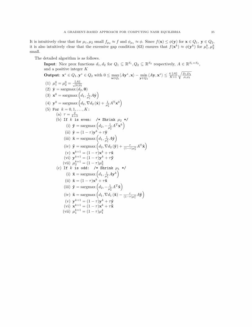
The detailed algorithm is as follows.Input: Nice prox functions d1, d2 for Q1 ⊆ RS1 , Q2 ⊆ RS2 respectively, A ∈ RS1×S2 ,and a positive integer KOutput: x∗ ∈ Q1,y∗ ∈ Q2 with 0 ≤ max

x∈Q1〈Ay∗,x〉 − min

y∈Q2〈Ay,x∗〉 ≤ 4 ‖A‖

K+1

√D1D2ρ1ρ2

(1) µ01 = µ0

2 = ‖A‖√ρ1ρ2

(2) y = sargmax (d2,0)(3) x0 = sargmax

(d1,

1µ0

1Ay)

(4) y0 = sargmax(d2,∇d2 (x) + 1

µ02ATx0

)(5) For k = 0, 1, . . . ,K:

(a) τ = 2k+3

(b) If k is even: /* Shrink µ2 */

(i) y = sargmax(d2,− 1

µk2ATxk

)(ii) y = (1− τ)yk + τ y

(iii) x = sargmax(d1,

1µk

1Ay)

(iv) y = sargmax(d2,∇d2 (y) + τ

(1−τ)µk2ATx

)(v) xk+1 = (1− τ)xk + τ x(vi) yk+1 = (1− τ)yk + τ y(vii) µk+1

2 = (1− τ)µk2

(c) If k is odd: /* Shrink µ1 */

(i) x = sargmax(d1,

1µk

1Ayk

)(ii) x = (1− τ)xk + τ x

(iii) y = sargmax(d2,− 1

µk2ATx

)(iv) x = sargmax

(d1,∇d1 (x)− τ

(1−τ)µk1Ay)

(v) yk+1 = (1− τ)yk + τ y(vi) xk+1 = (1− τ)xk + τ x(vii) µk+1

1 = (1− τ)µk1

a gradient-based approach for computing nash equilibria of

Documents