a gradient boosting approach to the kaggle load...
TRANSCRIPT

A gradient boosting approach to the Kaggle load forecasting competition
Souhaib Ben Taieb1 and Rob J Hyndman2
1 Machine Learning Group, Department of Computer Science, Faculty of Sciences, Universite Libre de Bruxelles2 Department of Econometrics and Business Statistics, Monash University, Clayton, VIC 3800, Australia
Abstract
We describe and analyse the approach used by Team TinTin (Souhaib Ben Taieb and Rob J Hynd-man) in the Load Forecasting track of the Kaggle Global Energy Forecasting Competition 2012. Thecompetition involved a hierarchical load forecasting problem for a US utility with 20 geographicalzones. The available data consisted of the hourly loads for the 20 zones and hourly temperaturesfrom 11 weather stations, for four and a half years. For each zone, the hourly electricity load fornine different weeks needed to be predicted without having the location of zones or stations. Weused separate models for each hourly period, with component-wise gradient boosting to estimateeach model using univariate penalised regression splines as base learners. The models allow for theelectricity demand to change with time-of-year, day-of-week, time-of-day, and on public holidays,with the main predictors being current and past temperatures as well as past demand. Team TinTinranked fifth out of 105 participating teams.
Keywords: short-term load forecasting, multi-step forecasting, additive models, gradient boosting,machine learning, Kaggle competition
1. Introduction
We participated in the Load Forecasting track of the Kaggle Global Energy Forecasting Competi-tion 2012 organised by the IEEE working group on Energy Forecasting (WGEF) (Hong et al., 2013).Team TinTin (Souhaib Ben Taieb and Rob J Hyndman) ranked fifth out of 105 participating teams.The competition involved a hierarchical load forecasting problem. We were required to backcast andforecast hourly loads (in kW) for a US utility with 20 geographical zones. Thus, 21 separate timeseries needed to be backcast and forecast: the 20 zonal level series, and the aggregate series.
Electricity demand is subject to a range of factors including weather conditions, calendar effect,economic activity and electricity prices. However we were required to use only temperatures andcalendar information. The available data consisted of the hourly loads for the 20 zones, and hourlytemperatures from 11 weather stations, from the first hour of 1 January 2004 to the sixth hour of 30June 2008. We are unaware of the location of the 20 zones and the 11 weather stations; in particular,we do not know which stations are located in or near which zones. Consequently, our task was tofind a model that takes temperature and calendar information as inputs, and predicts electricity loadas the output.
We used a separate model for each hourly period ending up with 24 different models for one daysince the electricity demand pattern is changing throughout the day. Each hourly model is estimatedusing component-wise gradient boosting (Buhlmann and Yu, 2003) with univariate penalised regres-sion splines (Eilers and Marx, 1996) as base learners together with an automatic variable selectionduring the fitting process. The models can be cast in the framework of additive models allowingnonparametric and non-linear terms. The models allow for the electricity demand to change withtime-of-year, day-of-week, time-of-day, and on public holidays. The main predictors were currentand past temperatures (up to a week earlier) and past demand (up to a week earlier).
Preprint submitted to International Journal of Forecasting July 18, 2013

Our approach has been influenced by the work of Fan and Hyndman (2012) who developed semi-parametric additive models with penalised spline functions for forecasting electricity demand invarious Australian states.
The paper is organised as follows. The next section presents the data analysis and preprocessingwe performed. Section 3 describes our forecasting methodology, clarifying the differences betweenin-sample and out-of-sample weeks. Section 4 presents our model together with the gradient boost-ing algorithm. The proposed model is analysed in Section 5. Section 6 provides some discussion andconclusions.
2. Data analysis and preprocessing
Figure 1 shows the average demand for all zones during the period of the data. The averagedemand varied greatly across zones with Zone 18 having the highest demand levels and Zone 4the least. By exploring the data, we noticed that Zones 3 and 7 contain identical data, and Zone 2contains values that are exactly 92.68% of the demand values in Zones 3 and 7. Also, Zone 10 has abig jump in demand in year 2008. Finally, Zone 9 contained very erratic demand patterns which didnot seem to relate to the temperature values.
Electricity demand is subject to a wide variety of exogenous variables including calendar effects.Figure 2 shows that there is a clear time-of-year effect in the demand data with peaks in mean de-mand around February and July, and troughs in April/May and October. In others words, winterand summer are showing high demand while fall and spring have lower demand.
Boxplots of the demand by day of week are shown in Figure 3. While the day-of-week effect isrelatively small, there is a drop in demand for the weekends. The average demand for each month
Gwh
Zone 4Zone 8Zone 5Zone 1
Zone 13Zone 14Zone 16Zone 10Zone 17Zone 15
Zone 9Zone 19Zone 20Zone 11Zone 12
Zone 2Zone 6Zone 3Zone 7
Zone 18
0 50 100 150 200
●
●
●
●
●
●
●
●
●
●
●
●
●
●
●
●
●
●
●
●
Figure 1: Average demand for each zone.
2

1000
1500
2000
2500
3000
Demand by time of year
Time of year
Tota
l Dem
and
(GW
)
Jan Feb Mar Apr May Jun Jul Aug Sep Oct Nov Dec
Figure 2: Total demand plotted against the time of year. The smoothed mean demand is shown as a red line.
and each day of the week is plotted in Figure 4. Because the day-of-week pattern is similar for allmonths, there is unlikely to be a strong interaction between day-of-week and time-of-year.
We look at the way demand changes with the time of day in Figures 5 and 6. Here hour 0 corre-sponds to 12am–1am, hour 1 corresponds to 1am–2am, and so on. The night-time pattern is similarfor the two plots, but there is a difference during the working hours (8am–5pm).
Figure 7 shows demand in Zone 18 plotted against current temperature from station 9. There isa clear non-linear relationship, indicating current temperature is an important predictor of demand.For temperatures above 20◦C, air conditioning usage drives demand, whereas for temperatures be-low 15◦C, heating drives demand. Similar but weaker relationships are seen in plots against laggedtemperatures. Due to thermal inertia in buildings, it is important to consider lagged temperaturesas well as current temperatures in any demand forecasting model. Figure 8 shows current demandplotted against lagged demand for different lags. We can see the relationship between these variablesdue to the serial dependence within the demand time series.
Before developing any forecasting models, we pre-processed the data to avoid some potentialproblems. First, we removed leap days to have 365 days for each year. This avoided problems withuneven seasonal periods, and resulted in only a small loss of information. Second, we took a logtransformation for the demand. This is to stabilise the variance of the time series across time. Therewere also some outliers and unusual features in the data which we corrected before proceeding.
We identified some outliers in site 8 for the temperature data, and replaced them with the dataof the same period in the closest site in terms of Euclidean distance.
Zone 4 had some outliers in demand. We used Loess for fitting and then classified a point yt as anoutlier if yt − yt >median(yt − yt) + k ∗MAD where yt is the Loess fit of yt, MAD is the mean absolutedeviation and k is chosen so the probability of an outlier is 0.002 under a normal distribution. Then,the outliers have been replaced by the mean of the data.
For Zone 10, there was a big jump in demand in year 2008. We computed the mean before thejump and the mean after the jump on the log-transformed data. Then we took the difference andremoved the jump in 2008. For the final forecasts, we restored the jump into the forecasts.
3

●●●●
●●●●●●●●●
●●●●●
●●
●●●●●●
●●
●●
●
●●●
●●●●●
●●
●
●●
●●●●
●
●
●●●
●
●
●●●
●●●
●
●
●●●●●
●
●●
●●
●●●●●●●
●●●●●●●●●●●●●●●●●
●●●
●●●●●●●●
●
●
●
●
●
●
●
●●●●●●
●●●●●
●
●●
●●
●●●●
●●●●●●
●
●●●●●●●●●●●●●●●●
●●●●●●●
●●
●●●
●●●●
●●
●●
●
●●●●●●●●
●
●●●●
●●●●●●●●●●●
●●●
●●
●●●●●●●●●
●●
●●
●
●
●
●●
●
●●●●●●
●●●●
●
●●●
●●
●●●
●●●●●●●●●●●●●●●●●●●
●●●
●●●●●●●●●●●
●●●●●●●●●●●●●●●●●●
●●
●●●●●●●●●●●●●●●●●●
Mon Tue Wed Thu Fri Sat Sun
1000
1500
2000
2500
3000
Day of week
Tota
l dem
and
(GW
)
Figure 3: Boxplots of total demand by day of week.
1300
1500
1700
1900
Mean demand by month and day of week
Tota
l dem
and
(GW
)
● ●
● ●
●
● ●
●
●
●
●
●
●
●
● ● ●●
●●
●
● ●
● ●
●
●
●
●
●● ●
●
●
●
●
●
●
●
●
●
●
●
●●
● ●
●
●
●
● ●
●●
●
●
●
●●
●●
●
●●
● ●●
●
●●
● ●
● ●
●●
●
●
●
●●
●●
●
Mon Tue Wed Thu Fri Sat Sun
Jan
Feb
Mar
Apr
May
Jun
JulAug
Sep
Oct
Nov
Dec
Figure 4: Average total demand (GW) by month and day of week.
4

●
●●●
●
●●●●
●
●
●●
●
●
●●
●
●
●
●
●●●●
●●
●●●
●
●
●●●
●
●
●●
●
●
●●
●
●
●
●
●●
●●
●●
●
●●●
●
●●
●
●●
●
●
●●
●
●
●
●
●●
●
●
●
●
●●●
●●●
●
●
●●●
●
●●
●
●●
●
●
●●
●
●
●
●●●
●
●
●
●●●
●●●
●
●
●●
●
●
●●●●●
●
●
●●
●
●
●
●●
●
●
●
●●●
●●●
●●
●
●●
●●●
●
●
●
●
●●
●
●
●●
●
●
●
●
●●
●
●●
●●
●
●●
●●●
●
●●●
●
●
●
●●
●
●●●
●
●
●
●
●
●●
●●
●●●●
●
●●
●●●●
●
●●●
●
●
●
●
●
●
●
●
●●
●
●
●
●
●
●
●
●
●
●
●●
●●
●
●●
●●●
●●●
●
●
●
●
●●
●
●●●
●
●
●
●
●
●
●●
●●● ●
●●●●●
●
●
●●●●●
●
●●
●
●
●●
●●●
●
●
●●●
●●●●●●
●●●
●
●●
●
●●●
●
●●●
●●●●●
●
●
●●
●●
●
●●
●
●
●●
●●
●
●
●●
●
●●
●●●●
●
●●●
●
●●●●
●●
●
●
●
0 1 2 3 4 5 6 7 8 9 11 13 15 17 19 21 23
1000
1500
2000
2500
3000
Weekdays
Hour of day
Tota
l dem
and
(GW
)
Figure 5: Boxplots of demand by time of day for Monday–Friday.
●●
●
●●
●●
●●●
●●
●
●
●
●●●
●●
●
●
●
●●●●●
●
●●●●
●●
●●●
●
●●
●●
●
●●
●●
● ●●●●
●●●
●
●●●
●
●●
●
●
●●
●
●
●
●
●
●
●
●●
●
0 1 2 3 4 5 6 7 8 9 11 13 15 17 19 21 23
1000
1500
2000
2500
Weekends
Hour of day
Tota
l dem
and
(GW
)
Figure 6: Boxplots of demand by time of day for Saturday–Sunday.
5

−10 0 10 20 30
100
200
300
400
500
Temperature (deg C)
Dem
and
(GW
)
Figure 7: Hourly demand (GW) plotted against temperature (degrees Celsius) for Zone 18 and station 9.
100 200 300 400 500
100
200
300
400
500
p−1
p
100 200 300 400 500
100
200
300
400
500
p−7
p
100 200 300 400
100
200
300
400
500
p−24
p
100 200 300 400 500
100
200
300
400
500
p−48
p
Figure 8: Current demand plotted against lagged demand for different lags for Zone 18.
6

3. Forecasting methodology
The competition involved a hierarchical load forecasting problem with 20 zonal level series, andthe aggregate series. We used a bottom-up approach, that is we forecast each zone independentlyand then we take the sum of the 20 zonal forecasts to obtain forecasts for the aggregate. For each ofthe twenty zones, we were required to backcast the demand for eight in-sample weeks for which thetemperature at various sites was provided.
Because we do not know which temperature site corresponds to which zone, the temperaturesfrom all sites are potential predictors in each model. We used a testing week (the last week of theavailable data) to determine which sites to use for each zone. Figure 9 gives the root mean squarederror (RMSE) obtained on the testing week using the real temperature (in blue) and the forecastedtemperature (in red) from the eleven sites for ten zones. We can see that the difference in forecastsobtained using the real temperature (in blue) at different sites can be huge. Consequently, whenforecasting the eight in-sample weeks, we use, for each zone, the site which minimises the error overthe testing week.
For the eight in-sample weeks, data was available before and after the week for demand andduring the week for the temperature. The data after each of the in-sample weeks is also usefulfor predicting the demand values during the in-sample weeks (although this is not possible in realforecasting operations). In order to use this data, we fitted two forecasting models. The first modelwas estimated in the usual way using data available up to the start of the in-sample week. The secondmodel reversed the time ordering of the data so we were back-casting using data available after theend of the in-sample week. We expect the forecasts to do best at the beginning of the week, andthe backcasts to do best at the end of the week, because they involve data closer to the days beingpredicted. So, after estimating the two sets of models, we took a weighted combination of both sets
of forecasts to produce the final forecasts. More precisely, if we denote y(F)t+h, the forward forecasts
and y(B)t+h, the backward forecasts with h = [1, . . . ,168], then the final forecasts are given by
yt+h = why(F)t+h + (1−wh)y(B)
t+h
where wh = sigmoid(−7 + 14∗h168 ) and sigmoid(x) = 1/(1 + e−x) is the sigmoid function.
Forecasts were also required for one out-of-sample week without temperature data. In contrastwith the in-sample weeks, temperatures were not provided for the out-of-sample week. So we hadto forecast the temperatures for this week and used these when forecasting demand during thatweek. We used the average temperature at the same period across the years as forecasts, shown inFigure 10. Differences between out-of-sample forecasts obtained using different temperature sitesare not as large as for the in-sample weeks as can be seen in Figure 9 (see red bars). This is becausewe do not have actual temperatures in that week, and our forecast temperatures have a smaller rangethan the actual temperatures. So, for out-of-sample forecasts, we average the forecasts obtained fromthe three best temperature sites when forecasting demand in order to reduce the variance of theforecasts. These sites are also shown in Figure 9.
Since the demand patterns varies greatly during the year and for computational convenience, wedid not use the whole demand data to estimate our models. Instead, for each of the available years,we used part of the data around the week to be forecast. More precisely, we computed the averagetemperature for the week to be forecast and, for each year, we select the 12 consecutive weeks aroundthis week which have the closest average temperature. Then we filtered the demand data by keepingthese 12 consecutive weeks of each year. For the out-of-sample week, for which we do not have theaverage temperature for the week to be forecast, we used the average temperature of the previousweek to perform the same calculations.
The above procedures was followed for all zones except zones 2, 7 and 9. Zones 3 and 7 containidentical data, and Zone 2 contains values that are exactly 92.68% of the demand values in Zones 3
7

9 4 6 8 10 7 3 1 5 11 2
Zone 18
Temperature site
RM
SE
010
000
3000
0
9 7 3 5 11 10 4 6 1 8 2
Zone 3
Temperature site
RM
SE
050
0015
000
9 7 3 5 11 10 6 4 1 8 2
Zone 6
Temperature site
RM
SE
050
0015
000
5 3 1 9 4 8 7 6 10 11 2
Zone 12
Temperature site
RM
SE
010
000
3000
0
5 3 9 1 4 8 7 6 10 11 2
Zone 11
Temperature site
RM
SE
050
0015
000
2500
0
9 11 6 10 4 8 3 7 5 2 1
Zone 20
Temperature site
RM
SE
040
0080
0012
000
10 6 8 1 4 9 7 3 5 11 2
Zone 19
Temperature site
RM
SE
050
0010
000
1500
0
6 10 4 8 1 7 9 3 11 2 5
Zone 15
Temperature site
RM
SE
020
0060
0010
000
4 8 6 1 10 3 9 5 7 11 2
Zone 17
Temperature site
RM
SE
010
0030
0050
00
1 4 8 3 9 5 6 10 7 11 2
Zone 10
Temperature site
RM
SE
050
0010
000
1500
0
Figure 9: Root mean square error (RMSE) over the testing week using real temperature (in blue) and forecasted temperature(in red). The sites are ranked according to the RMSE when using real temperature.
and 7. Consequently, we do not fit separate models for Zones 2 and 7, instead we use the forecastsfrom Zone 3 to compute forecasts for Zones 2 and 7. And for Zone 9, we used the average of thesame hour for every day of the week over the entire data set to obtain forecasts for each period as wedidn’t find any temperature-related patterns.
4. Forecasting model
One of the earliest electricity forecasting competitions was won by Ramanathan et al. (1997)using a separate regression model for each hour of the day. This idea has subsequently been used byFay et al. (2003); McSharry et al. (2005); Fan and Chen (2006) and Fan and Hyndman (2012).
We follow the same approach and have a separate model for each hour of the day. These modelsare used recursively to produce the 168 required forecasts (24 hours multiplied by 7 days). That is,
8

Station : 1
Time
fore
cast
s
0 50 100 150
7075
8085
90Station : 2
Time
fore
cast
s
0 50 100 150
6065
7075
80
Station : 3
Time
fore
cast
s
0 50 100 150
6570
7580
85
Station : 4
Timefo
reca
sts
0 50 100 150
7075
8085
90
Station : 5
Time
fore
cast
s
0 50 100 150
6570
7580
85
Station : 6
Time
fore
cast
s
0 50 100 150
7075
8085
Station : 7
Time
fore
cast
s
0 50 100 150
7075
8085
Station : 8
Time
fore
cast
s
0 50 100 150
7075
8085
90
Station : 9
Time
fore
cast
s
0 50 100 150
6570
7580
85
Station : 10
Time
fore
cast
s
0 50 100 150
6570
7580
85
Station : 11
Time
fore
cast
s
0 50 100 150
6065
7075
8085
Figure 10: Forecasts of temperature for the eleven stations.
9

we first produce the forecasts of the next day and then, use them as inputs to make forecasts for theday after. We also added the observations from the previous hour and the next hour in order to havemore data. That is, when estimating the model for hour p, we used data from hours p−1, p and p+1.
We fit a model of this form for each hour of the day, for each zone, and for each of the nineweeks to be forecast. We ended up with 24× 17× 9 = 36721 models to estimate with datasets havingapproximately 1000 observations and 43 input variables. The main predictors of the models arecurrent and past temperatures (up to a week earlier) and past demand (up to a week earlier). Inaddition, the models allow for the demand to change with time-of-year, day-of-week, time-of-day,and on public holidays.
Each regression uses a nonparametric additive model with penalised regression splines. Component-wise gradient boosting is used to estimate each model including variable selection during the fittingprocess. Both aspects are detailed in the following sections.
4.1. Non-parametric additive models
We use nonparametric additive models for forecasting electricity demand. These models arein the regression framework but with some non-linear relationships. In particular, the proposedmodels allow nonlinear and nonparametric terms using the framework of additive models (Hastieand Tibshirani, 1995).
The demand in hour p on day t is modelled with
yt,p = cp(t) + fp(yt,p) + gp(zt,p) + εt , (1)
where• yt,p denotes the demand on day t in hour p;• cp(t) models all calendar effects (including time-of-year, day-of-week, holidays, etc.);• fp(yt,p) models the effect of recent demand variables where yt,p is a vector of past demands,
prior to hour p on day t;• gp(zt,p) models the temperature effects where zt,p is a vector of recent temperatures variables at
one of the temperature sites, prior to and including hour p on day t; and• εt denotes the model error at time t.
We fit separate models of this form for each zone and all in-sample and out-of-sample weeks.
4.1.1. Calendar effectsThe calendar effects term, cp(t), includes annual, weekly and daily seasonal patterns as well as
public holidays.• The day-of-week effect was modelled with a factor variable, taking a different value for each
day of the week.• The holiday effect was modelled with a factor variable, taking value zero on a non-work day2,
some non-zero value on the day before a non-work day and a different value on the day after anon-work day.
• The time-of-year effect was estimated using a simple first-order Fourier approximation (onesine and one cosine variables). A more complicated time-of-year effect was not necessary aseach model only included data within a 12 week period.
1There are only 17 zones to be modelled because of the relationship between Zones 2, 3 and 7, and because we use adifferent approach for Zone 9.
2We used the US federal holidays as listed in US Office of Personnel Management website: http://www.opm.gov/
Operating_Status_Schedules/fedhol/2008.asp
10

4.1.2. Temperature effectsDue to thermal inertia in buildings, it is important to consider lagged temperatures as well as
current temperatures in any demand forecasting model. The function gp(zt,p) models the effects ofrecent temperatures on the aggregate demand where zt,p includes
• The current temperature and temperatures from the preceding 12 hours, and for the equivalenthour on each of the previous two days;
• The minimum and maximum temperature in both the last 24 hours and the previous day;• The average temperature for the previous day, the day preceding the previous day and the last
seven days.Recall that when forecasting the eight in-sample weeks, the temperatures from the site which
gave the best forecasts (on the testing week) for each zone were used. When forecasting the out-of-sample week, the demand forecasts obtained using the best three temperature sites were averaged.
4.1.3. Lagged demand effectsWe incorporate recent demand values into the model via the function fp(yt,p) where yt,p includes• Lagged demand for each of the preceding 12 hours, and for the equivalent hour in each of the
previous two days. For example, when predicting demand at 4pm, we use lagged demand from4am to 3pm, as well as lagged demand at 4pm on the preceding two days.
• The minimum and maximum demand in the last 24 hours.• The average demand for the last seven days.
By doing this, the serial correlations within the demand time series can be captured within the model,and the variations of demand level throughout the time can be embedded into the model as well.
Finally, we did not necessarily use all the previous predictors in each model, but these were allcandidate variables in our models. The process of selecting variables is described in the next sectiontogether with the gradient boosting algorithm.
4.2. Component-wise gradient boosting with penalised splines
Boosting is a prediction algorithm stemming from the machine learning literature based on theidea of creating an accurate learner by combining many so-called “weak learners”. Since its inceptionin 1990 (Schapire, 1990; Freund, 1995; Freund and Schapire, 1996), Boosting has attracted muchattention due to its excellent prediction performance in a wide range of applications both in themachine learning and statistics literatures (Schapire and Freund, 2012). The improved performanceof boosting seems to be associated with its resistance to overfitting which is still under investigation(Mease and Wyner, 2008; Mease, 2008).
The gradient descent view of boosting (Friedman and Hastie, 2000; Friedman, 2001) has con-nected boosting to the more common optimisation view of statistical inference while previous workfocused on bounding the generalisation error via the VC dimension and the distribution of so-calledmargins (Schapire et al., 1998). Gradient boosting (Friedman, 2001) interprets boosting as a methodfor function estimation from the perspective of numerical optimisation in function space.
Buhlmann and Yu (2003) developed component-wise gradient boosting to handle high-dimensionalregression problems by selecting one variable at each iteration of the boosting procedure. We refer toSchapire and Freund (2012) and Buhlmann and Hothorn (2007) for a general overview on boosting.
For all our regression tasks, we used component-wise gradient boosting (Buhlmann and Yu, 2003;Buhlmann, 2006) with penalised regression splines (P-splines) (Eilers and Marx, 1996). By doingso, we take advantage of the good performance and the automatic variable selection of the boostingalgorithm. In addition, P-splines allow us to have smooth estimation of the demand. We now providemore details about the procedure we implemented.
Notice that expression (1) can be rewritten as
yt,p = Fp(xt) + εt,p.
11

where xt = [t,yt,p,zt,p] contains all potential predictors to be considered in the model. Our goal is toestimate the function Fp : Rd → R for a given loss function. Since, the forecasting accuracy for thecompetition was evaluated by weighted root mean square error, we used the quadratic loss function.Estimation of the function Fp based on a sample dataset {(yt,p,xt)}Tt=1 reduces to minimising
Fp = argminFp
1T
T∑t=1
(yt,p −Fp(xt))2.
Gradient boosting estimates Fp in a stagewise manner. We let F(m)p (xt) denote the estimation of Fp
at the mth stage, where m = 0,1, . . . ,M. The process begins with F(0)p (x) = yp where yp is the mean
demand for hour p. Then the model is updated using
F(m)p (xt) = F(m−1)
p (xt) + νhm(xt; θm),
where hm(xt; θm) is the weak learner estimate at the mth stage with parameters θm and ν ∈ [0,1] isa shrinkage parameter. Gradient boosting with the quadratic loss is also called L2Boost (Buhlmannand Yu, 2003).
Let us note hm(xt) as a shorthand for hm(xt; θm). Given an estimation F(m−1)p , each additional term
hm(xt) is obtained by computing the negative gradient
umt,p = −12∂(yt,p −F(xt))2
∂F(xt)
∣∣∣∣∣F(x)=F(m−1)
p (x)= (yt,p −F
(m−1)p (xt))
which gives the steepest descent direction. Then, a regression is applied on {umt,p,xt}Tt=1 by the weaklearner, i.e.
θm = argminθ∈Θ
T∑t=1
[umt,p − hm(xt;θ)]2 (2)
In other terms, hm(xt) is selected to best predict the residuals from the previous model F(m−1)p (xt).
Finally, the solution is given by
Fp(xt) = F(M)p (xt) = h0(xt) +
M∑m=1
νhm(xt) (3)
where the estimation of Fp is continuously improved by an additional component (or boost) νhm atstage m and the hyperparameter M prevents overfitting by limiting the number of components.
From expression (3), we can see that the boosting procedure depends on two hyperparameters:ν, the shrinkage parameter and M, the number of components (or number of stages). The value of νaffects the best value forM, i.e. decreasing the value of ν requires a higher value forM. Since they canboth control the degree of fit, we should ideally find the best value for both of them by minimisingsome model selection criterion. However, Friedman (2001) shows that small values of ν are betterin terms of less overfitting of the boosting procedure. Hence, there is only one hyperparameterremaining for which the best value need to be selected (Buhlmann and Yu, 2003).
In expression (2), the weak learner is estimating the model parameters using all the predictorssimultaneously A better procedure can be used when having many predictors: component-wise gra-dient boosting (Buhlmann and Yu, 2003; Buhlmann, 2006). The key idea is to use the weak learnerwith one variable at a time and select the one with the largest contribution to the fit. In other terms,
12

expression (2) is replaced by the following procedure:
1. θ(k)m = argmin
θ∈Θ
∑Tt=1[umt,p − hm(xkt;θ)]2 where xkt is the kth variable of xt and k = 1, . . . ,d.
2. km = argmink∈1,...,d
∑Tt=1[umt,p − hm(xkt; θ
(k)m )]2.
3. Use θ(km)m at the mth stage.
Then, the final solution is expressed as
Fp(xt) = h0(xk0t) +M∑m=1
νhm(xkmt) (4)
where hm is function of the kmth predictor.In our implementation, we used P-splines with 20 equally spaced knots and four degrees of free-
dom for the weak learner hm(xkmt) terms. For the hyperparameters values, we set the value of νto 0.15 and the maximum number of components (or stages) M to 500. Our implementation of themodel depended on the mboost package for R (Hothorn et al., 2012). We used the gamboost functionwith the following values for the mboost_control parameters: nu=0.15 and mstop=500. For the baselearners, we used the bbs function for numerical variables and the bols function for factor variables.Finally, we select the best number of stages M(M ∈ {1, . . . ,mstop}) using the cvrisk function with5-fold cross-validation.
5. Model analysis
In this section, we analyse and interpret the results of the proposed forecasting model to shedlight about its attractive features.
Figure 11 gives the root mean squared error (RMSE) obtained for the different zones on the testingweek. Zones that have higher errors are also zones with high average demand (see Figure 1). Thissuggests that zones with high average demand will carry a higher weight in the final error.
Figure 12 gives the true hourly demand together with the fitted values for an increasing numberof boosting iterations. Recall that gradient boosting is a stagewise fitting procedure which dependson an hyperparameters M (the number of boosting iterations), as shown in formula (4). We can seethat the first iterations significantly reduce the error of the model while the final iterations are lessand less contributing to the model. This confirms the theoretical analysis performed in (Buhlmannand Yu, 2003) where the authors proof that the bias decreases exponentially fast and the varianceincreases with exponentially diminishing terms as the number of boosting iteration M increases.
One of the attractive feature of the component-wise boosting algorithm is the automatic variableselection induced by the procedure at each iteration. That is, among all the potential predictorswhich are given in Table 1, few will be selected and contribute to each hourly model. See Section 4.1for a more detailed description of the different predictors.
Note that the final solution of the boosting procedure, given in formula (4), can be rewritten as
Fp(xt) =M∑m=0
νhm(xkmt) =∑
k∈{1,...,d}
∑{m:km=k}
νhm(xkmt)︸ ︷︷ ︸H(xkt)
=∑
k∈{1,...,d}H(xkt),
13

Zone 4Zone 8Zone 5Zone 13Zone 17Zone 1Zone 14Zone 16Zone 15Zone 19Zone 2Zone 6Zone 20Zone 3Zone 7Zone 10Zone 11Zone 12Zone 18
●
●
●
●
●
●
●
●
●
●
●
●
●
●
●
●
●
●
●
1
0 2000 4000 6000 8000
WRMSE
Figure 11: Root mean squared error (RMSE) obtained for each zone on the testing week.
Id Variable Id Variable Id Variable Id Variable1 day of the week 12 demand[t-8] 23 temp.[t+h-2] 34 temp.[t+h-13]2 holiday 13 demand[t-9] 24 temp.[t+h-3] 35 temp.[t+h-25]3 time of year (sin) 14 demand[t-10] 25 temp.[t+h-4] 36 temp.[t+h-49]4 time of year (cos) 15 demand[t-11] 26 temp.[t+h-5] 37 min. temp. (prev 1)5 demand[t-1] 16 demand[t-12] 27 temp.[t+h-6] 38 min. temp. (prev 2)6 demand[t-2] 17 demand[t+h-25] 28 temp.[t+h-7] 39 max. temp. (prev 1)7 demand[t-3] 18 demand[t+h-49] 29 temp.[t+h-8] 40 max. temp. (prev 2)8 demand[t-4] 19 min. demand (prev 1) 30 temp.[t+h-9] 41 avg. temp. (prev 1-7)9 demand[t-5] 20 max. demand (prev 1) 31 temp.[t+h-10] 42 avg. temp. (prev 1)10 demand[t-6] 21 avg. demand (prev 1-7) 32 temp.[t+h-11] 43 avg. temp. (prev 3)11 demand[t-7] 22 temp.[t+h-1] 33 temp.[t+h-12] – –
Table 1: Description of all potential predictors. Forecasts are from demand[t-1] to demand[t+h-1] where h ∈ {1, . . . ,24}.
where H(xkmt) is the relative contribution of the variable k to the final model and d is the number ofinitial predictors (the dimensionality of xt).
Let us define the model without the effect of predictor j as
F(−j)p (xt) =
∑k∈{1,...,d}\{j}
H(xkt),
and the corresponding squared error as
E(−j) =T∑t=1
(yt −F(−j)p (xt))
2.
14

12.0 12.2 12.4 12.6 12.8
12.0
12.2
12.4
12.6
12.8
M=0
Hourly demand
Fitt
ed
● ●● ● ●● ●●● ● ●● ●● ● ● ●● ● ●● ● ●● ● ●● ● ●● ● ●● ●●● ● ●● ● ●● ●●● ● ●● ● ●● ● ●● ● ●● ● ●● ● ●● ● ●● ● ●● ● ●● ● ●● ●●● ● ●● ● ●● ● ●● ● ●● ● ●● ● ●● ● ●● ● ●● ● ●● ● ●● ● ●● ● ●● ● ●● ● ●● ● ●● ● ●● ● ●● ● ●● ● ●● ●●● ●●● ●● ● ● ●● ● ●● ● ●● ● ●● ● ●● ● ●● ● ●● ● ●● ● ●● ●●● ●●● ● ●● ● ●● ● ●● ● ●● ● ●● ● ●● ● ●● ●●● ●●● ● ●● ● ●● ● ●● ● ●● ● ●● ●●● ● ●● ● ●● ● ●● ● ●● ● ●● ● ●● ● ●● ● ●● ● ●● ● ●● ● ●● ● ●● ● ●● ● ●● ● ●● ● ●● ● ●● ● ●● ● ●● ● ●● ●● ● ● ●● ● ●● ● ●● ● ●● ● ●● ● ●● ● ●● ● ●● ● ●● ● ●● ● ●● ● ●● ● ●● ● ●● ● ●● ● ●● ● ●● ● ●● ● ●● ● ●● ● ●● ● ●● ● ●● ● ●● ● ●● ● ●● ● ●● ● ●● ● ●● ● ●● ● ●● ● ●● ● ●● ● ●● ● ●● ● ●● ● ●● ● ●● ● ●● ● ●● ● ●●●● ● ● ●● ● ●● ● ●● ● ●● ● ●● ● ●● ● ●● ● ●● ● ●● ●● ● ● ●● ● ●● ● ●●● ●● ● ●● ● ●● ● ●● ●● ● ● ●● ● ●● ● ● ● ● ●●● ●● ● ●● ● ●● ● ●● ● ●● ● ●● ● ●● ●●● ● ●● ● ●● ● ●● ● ●● ● ●● ● ●● ● ●● ● ●● ● ●● ● ●● ● ●● ● ●● ●●● ● ●● ● ●● ● ●● ● ●● ● ●● ● ●● ● ●● ● ●● ● ●● ● ●● ● ●● ● ●● ●●● ●●● ● ●● ● ●● ● ●● ● ●● ● ●● ● ●● ● ●● ● ●● ● ●● ● ●● ● ●● ● ●● ● ●● ● ●● ● ●● ● ●● ● ●● ● ●● ● ●● ● ●● ● ●● ● ●● ● ●● ● ●● ● ●● ● ●● ● ●● ● ●● ● ●● ● ●● ● ●● ● ●●●●●●●● ●●● ● ●● ● ●●●●● ●●● ● ●● ● ●● ● ●● ● ●● ● ●● ● ●● ● ●● ● ●● ● ●● ● ●● ● ●● ● ●● ● ●● ● ●● ● ●● ● ●● ● ●● ● ●● ● ● ● ● ●● ● ●● ● ●● ● ●● ● ●● ● ●● ● ●● ● ●● ● ●● ● ●● ● ●● ● ●● ● ●● ● ●● ● ●● ● ●● ● ●● ● ●● ● ●● ● ●● ● ●● ● ● ● ● ●● ● ●● ● ●● ● ●● ● ●● ● ●● ● ●● ● ●● ● ●● ● ●● ● ●● ● ●● ● ●● ● ●● ● ●● ● ●● ● ●● ● ●● ● ●● ● ●● ● ●● ● ●● ● ●● ● ●● ● ●● ●●● ● ●● ●●● ● ● ● ● ●● ● ●● ● ●● ● ●● ● ●● ● ●● ● ●● ● ●● ● ●● ● ●● ● ●● ● ●● ● ●● ● ●● ● ●● ● ●● ● ●● ● ●● ● ●● ● ●● ● ●● ● ●● ● ●● ● ●● ● ●● ● ●● ● ●● ● ●● ● ●● ● ●● ● ●● ● ●● ● ●● ● ●● ● ●● ● ●
12.0 12.2 12.4 12.6 12.8
12.0
12.2
12.4
12.6
12.8
M=1
Hourly demand
Fitt
ed
●●
●●
●
● ●●
● ●●
● ●●●
●●●
● ●
● ● ●●●
●●
●●
●● ●
● ●●● ●
●●●
●
● ●●●●
●
●●
●
●● ●
●● ●
●● ●
● ●●●
●●
●●
●●
●●
●●
●
● ●●●
●●
●● ●
●
● ●
●●
●
●
● ●
●●
●●
●●
●● ●
●●
●
●●
●
●● ●
●● ●
●●
●
● ● ●●
●●
●●
●●
●●
●●
●
●●
●
● ●●● ●●● ●●
● ●●
● ●●
●● ●●
●●
●●
●
●● ●
●●
●
● ●
●●●
●
● ●●
● ●●●● ●●
●●
●●
●
●●
●
●●
●
● ●●
● ● ●● ●●●
●●●●
●
●● ●●
●●
●●
●
●
●
●
● ●●
●● ●
●
●●
●
●●
● ●●
●●
●● ●
●●
●●
●●
●
●●
●
●●
●
●
●●
●●
●
●
●●
●●
●●● ●
●
● ●
●● ●
●●
●
●● ●
●● ●
● ●●
●●
●
●●
●●
●●
●● ●
● ●●
●●
●●
●●
●● ●
● ● ●
●● ●●
●●
●
●●
●●
●●
●●
●●
●
● ●●
● ●●●
●●
●●
●●
●●
●●
●
●● ●
●●
●
●●
●
●● ●
●●
●
●
●
●●
●●
●
● ●
● ● ●●
● ●● ●
●● ● ●
●●
●●●
●
●●
●
●
●●
●
●●
●●
●
●●
●●
● ●
●●● ●●
●●
●
●
●
●●
●
●●
●●
●
●●
●
● ● ●
● ●●
●●
●
● ●● ●●
●●
●●
●
●●
●●
●●
●●
●● ●
●●
●
● ●●●
●●
● ●●
● ●● ●
●●
●● ●
●
●
●
●●
●
●
●●
●
●●
●
●
●
●
●●
●●
●
● ● ●● ● ●● ●●
● ●●
●●
●
●
● ●
●●
●
●●
●●
●
●
● ● ●●
●●
●●
●
● ●●●● ●
●● ●●
●●
●
●●
●●
●
●●
●
●●
●
● ●
●
●●
●●●
●●
●●
●
●●
●●●
●●
●●
●
●
●● ●
● ● ●●●
●
● ●●
●
●●
●
●●
●
●●
●●
●
●●
●
●●
●
●
●●
● ●●
●● ●
●●
●
●●
●●
●●
●●
●
●●
●
●●
●●
●●
●●
●
● ●●
●
●●
●
●●
●●
●
●
●●
●
●
●
●
●●●
●●
●●
●
●● ●
●●●
●●●● ●●●● ●● ● ●
●●●●●●
●●
●
● ● ● ●
●●●
●●
●●
●
● ●●
●●
●
● ● ●●
● ●● ● ●● ●
●●
●●
●●
●
●●
●
●●
●
● ●●
● ● ●
● ● ●●
●● ●
●●
● ●●●
● ●●
●●
●
●
●
●●
●
●
●●
●●
●
●● ●●
●●
●●
●●
●
●
●●
●
●●
●
●●
●
●●
●
● ●●
●●
●●
●
●
●● ●
●● ●
● ● ● ●●
●
●
●
●
●
●
●
●●
●
● ●●●
●●
●●
●
●●
●
●
●
●
●
●●
●●
●
●●
●●●
●●
●●
●●
●
●● ●
●●
●
●
●●
●
●●
●●
●
●●
●
●●
●
●
●●
● ●●
●●
●
● ●●● ● ●
● ●●● ● ● ●●
●●
●●
●● ●
●●
●
● ●●
●●
●
● ●●
●●
●
●● ●
●●
●●
●●
●
●●
●
●●
●
●●
●●
●
●
●●
●●
●
●●
●●● ●
●●
●
●●
●
●●
●
●
●●
●●
●
●● ●
●●
●●
●●
●●
●
●●
●
●●
●
●● ●
●●
●●
●●
●
●●
●●
●
●●
●
12.0 12.2 12.4 12.6 12.8
12.0
12.2
12.4
12.6
12.8
M=2
Hourly demand
Fitt
ed ●
●
●
●●
● ●●
●●
●
●●●
●
●
●●
● ●
● ● ●●
●
●
●
●●
●
● ●
●●●
●●
●●
●
●
● ●●●
●
●
●
●
●
●
● ●
●
●●
●
●●
● ●●
●
●●
●
●●
●
●
●
●
●●
● ●●●
●
●
●
● ●
●
● ●
●
●
●
●
●●
●
●●
●
●●
●
● ●●
●
●
●
●●
●
● ●
●
● ●
●
●
●
● ●●
●
●
●
●
●●
●
●●
●●
●
●
●●
● ●●● ●●● ●●
● ●●
● ●
●
●
●●
●
●●
●
●●
●
● ●
●
●●
●●
●●●
●
● ●
●
●●●●
● ●
●
●
●
●
●
●
●
●
●
●
●
●
●●
●
●● ●
● ●●●●●●
●
●
●
●●
●
●
●
●
●
●
●
●
●
● ●●
●
●●
●
●
●
●
●
●
●●
●
●●
●
●●
●
●
●
●
●
●
●
●
●
●
●
●●
●
●
●
●
●●
●
●●
●
●
●●
●●
●
●●
●
● ●
●
●●
●● ●
●
●●
● ●●
●
●●
●
●
●●
●●
●● ●
●●
●
●
●●
●
●
●
●
● ●
● ● ●
●
● ●●
●●
●
●●
●
●
●
●●
●
●
●●
●●
●
●●
●●
●
●
●
●
●
●●
●
●
●
●
●●
●
●
●
●
●
●●
●
●●
●
●
●
●
●
●
●
●●
●
●●
●● ●
●
● ●
●●
●
● ●●
●
●
●●
●
●
●
●
●
●
●
●
●
●
●
●
●●
●
●
●
●
● ●
●●●●
●●
●
●
●
●
●
●
●
●
●
●
●
●
●
●
●
●●
●
● ●
●
●
●●
● ●●●
●
●●
●●
●
●
●
●●
●
●●
●
●
●●
●
●
●
● ●●
●
●
●
●●
●
●●
● ●
●●
●
●●
●
●
●
●
●
●
●
●
●
●
●●
●
●
●
●
●
●
●●
●
● ● ●● ●●
● ●
●
●●
●
●
●●
●
● ●
●
●●
●
●
●
●
●
●
● ●●
●
●
●
●
●●
● ●●●
● ●
●
●●
●
●
●
●
●
●
●
●
●
●
●
●
●●
●
● ●
●
●
●
●●●
●
●
●●
●
●●
●
●
●
●
●
●
●●
●
●
● ●
● ● ●●
●
●
● ●
●
●
●●
●
●
●
●
●●
●
●●
●
●
●
●
●
●
●
●
●
● ●
●
●
●●
●
●
●
●
●
●●
●●
●
●
●
●
●
●
●
●
●
●
●
●●
●●
●●
●
●
●
●
●
●
●
●
●
●
●
●
●
●
●
●
●
●●●
●
●
●
●
●
●
● ●
●●●
●●●●●●●
●●
●● ●
●●●●●
●
●
●
●
● ●●
●
●●●
●
●
●
●
●
● ●
●
●
●●
● ● ●
●
● ●●
●●●
●
●●
●
●
●
●
●
●
●●
●
●
●
● ●
●
●●
●
●●
●
●
●●
●
●
●
●●
●●
● ●
●
●
●
●
●
●
●
●
●
●
●
●
●●
●
●
●●●
●●
●
●●
●
●
●
●
●●
●
●
●
●
●
●
●●
●
● ●
●
●●
●
●
●
●
●
● ●
●●
●
●●
●●
●
●
●
●
●
●
●
●
●●
●
●●
●●
●
●
●
●
●
●
●
●
●
●
●
●
●
●
●●
●
●
●
●●
●
●
●
●
●
●●
●
●
● ●
●
●
●
●
●
●
●
●●
●
●
●
●
●
●
●
●●
●
●●
● ●
●
●
●
●
● ●●●
● ●
● ●●●
●●
●
●
●
●
●
●
●
● ●
●
●
●
●●
●
●
●●
●●
●
●
●●
●
● ●
●
●
●
●●
●
●
●
●
●
●
●
●
●
●
●
●
●
●
●
●
●
●
●
●
●●●
●●
●
●
●
●
●
●
●
●
●
●
●
●
●
●
●
●● ●
●
●●
●
●
●
●
●●
●
●●
●
●
●
●
● ●
●
●
●●
●
●
●
●●
●
●
●
●
●
●
12.0 12.2 12.4 12.6 12.8
12.0
12.2
12.4
12.6
12.8
M=5
Hourly demand
Fitt
ed ●
●
●
●
●
●●
●
●
●
●
●●●
●
●
●●
●
●
●
●●
●
●
●
●
●
●
●
●
●
●
●●
●
●
●●
●
●
●
●●
●
●
●
●
●
●
●
●
●
●
●
●
●
●
●
●
●
●
●
●
●
●
●
●
●
●
●
●
●
●
●●●
●
●
●
●
●
●
●
●●
●
●
●
●
●
●
●
●
●
●
●
●
●
●
●
●
●
●
●
●
●
●
●
●
●
●
●
●
●
●
●●
●
●
●
●
●
●
●
●
●
●
●
●
●
●
●
●
● ●●
● ●●● ●●
●●
●
●
●
●
●
●
●
●
●
●
●
●
●
●
●
●
●
●
●
●
●
●●
●
●
●
●
●
●
●●
●
●●
●
●
●
●
●
●
●
●
●
●
●
●
●
●
●
●
●●
●●●
●
●●●
●
●
●
●
●
●
●
●
●
●
●
●
●
●
● ●●
●
●
●
●
●
●
●
●
●
●
●
●
●
●
●
●
●
●
●
●
●
●
●
●
●
●
●
●
●
●
●
●
●
●
●
●
●
●
●
●
●
●
●
●
●
●
●
●
●
●●
●
●
●
●
●
●
●
●
●
●
●●
●
●
●
●
●
●
●
●
●
●
●
●
●
●
●
●
●
●
●
●
●
●
●
●
●
●●
●
●
●●
●
●
●
●
●
●
●
●
●
●
●
●
●
●
●
●
●
●
●
●
●
●
●
●
●
●
●
●
●
●
●
●
●
●
●
●
●
●
●
●
●
●
●
●
●
●
●
●
●
●
●
●
●
●
●
●
●
●
●
●
●●
●
●
●
●●
●
●
●
●●
●
●
●
●
●
●
●
●
●
●
●
●
●
●
●
●
●
●
●
●
●●● ●
●
●
●
●
●
●
●
●
●
●
●
●
●
●
●
●
●
●
●
●
●
●
●
●
●
●
●●● ●
●
●●
●
●
●
●
●
●
●
●
●
●
●
●
●
●
●
●
●
● ●
●
●
●
●
●
●
●
●
●
● ●
●
●
●●
●
●
●
●
●
●
●
●
●
●
●
●
●
●
●
●
●
●
●
●
●
●
●●
●
●
●
●
●
●
●
●
●
●
●
●
●
●
●
●
●
●
●
●
●
●
●
●
●
●
●
●
●
●
●
●
●
●
● ●●
●
●●
●
●
●
●
●
●
●
●
●
●
●
●
●
●
●
●
●
●
● ●
●
●
●
●●
●
●
●
●
●
●
●
●
●
●
●
●
●
●
●
●
●
●
●
●
●●
●
●
●
●
●
●
●
●
●
●
●
●
●
●
●
●
●
●
●
●
●
●
●
●
●
●
●
●
●●
●
●
●
●
●
●
●
●
●
●
●
●
●
●
●
●
●
●
●
●
●
●
●
●
●
●
●
●
●
●
●
●
●
●
●
●
●
●
●
●
●
●
●
●
●
●
●
●
●
●
●
●
●
●
●
●
●●
●
●●
●●●
●●●●
●
●
●
●●
●●●
●
●
●
●
●
●
●●
●
●
●
●
●
●
●
●
●
●
●●
●
●
●
●
●●
●
●
●
●
●
●
●●
●
●
●
●
●
●
●
●
●
●
●
●
●
●
●
●
●
●
●
●
●
●
●
●
●
●
●
●
●
●
●
●
●
●
●
●
●
●
●
●
●
●
●
●
●
●
●
●
●
●
●
●
●
●
●
●
●
●
●
●
●
●
●
●
●
●
●
●
●
●
●
●
●
●
●●
●
●
●
●
●
●
●
●
●
●
●
●
●
●
●
● ●
●
●
●
●
●
●
●
●
●
●
●
●
●
●
●
●
●
●
●
●
●
●
●
●
●
●
●
●
●
●
●
●
●
●
●
●
●
●
●
●
●
●
●
●
●
●
●
●
●
●
●
●
●
●
●
●
●
●
●
●
●
●
●
●
●
●
●
●
●
●
●
●
●
●
●●
●
●
●●
● ●●
●●
●
●
●
●
●
●
●
●
●
●
●
●
●
●
●
●
●
●
●
●
●
●
●
●
●
●
●
●
●
●
●
●
●
●
●
●
●
●
●
●
●
●
●
●
●
●
●
●
●
●
●
●
●
●
●
●
●
●
●
●
●
●
●
●
●
●
●
●
●
●
●
●
●
●
●
●
●
●
●
●
●
●
●
●
●
●
●
●
●
●
●
●
●●
●
●
●
●
●
●
●
●
●
●
●
●
●
●
●
12.0 12.2 12.4 12.6 12.8
12.0
12.2
12.4
12.6
12.8
M=10
Hourly demand
Fitt
ed
●
●
●
●
●
●
●
●
●
●
●
●
●
●
●
●
●
●
●
●
●
●
●
●
●
●
●
●
●
●
●
●
●
●
●
●
●
●●
●
●
●
●●
●
●
●
●
●
●
●
●
●
●
●
●
●
●
●
●
●
●
●
●
●
●
●
●
●
●
●
●
●
●
●
●
●
●
●
●
●
●
●
●
●
●
●
●
●
●
●
●
●
●
●
●
●
●
●
●
●
●
●
●
●
●
●
●
●
●
●
●
●
●
●
●
●
●
●
●
●
●
●
●
●
●
●
●
●
●
●
●
●
●
●●●
●●●
●●
●
●
●
●
●
●
●
●
●
●
●
●
●
●
●
●
●
●
●
●
●
●
●
●
●
●
●
●
●
●
●
●
●
●
●
●
●
●
●
●
●
●
●
●
●
●
●
●
●
●
●
●
●
●
●
●●●
●
●●●
●
●
●
●
●
●
●
●
●
●
●
●
●
●
●●
●
●
●
●
●
●
●
●
●
●
●
●
●
●
●
●
●
●
●
●
●
●
●
●
●
●
●
●
●
●
●
●
●
●
●
●
●
●
●
●
●
●
●
●
●
●
●
●
●
●
●
●
●
●
●
●
●
●
●
●
●
●
●
●
●
●
●
●
●
●
●
●
●
●
●
●
●
●
●
●
●
●
●
●
●
●
●
●
●
●
●
●
●
●●
●
●
●
●
●
●
●
●
●
●
●
●
●
●
●
●
●
●
●
●
●
●
●
●
●
●
●
●
●
●
●
●
●
●
●
●
●
●
●
●
●
●
●
●
●
●
●
●
●
●
●
●
●
●
●
●
●
●
●
●
●
●
●
●
●
●
●
●
●
●
●
●
●
●
●
●
●
●
●
●
●
●
●
●
●
●
●
●
●
●
●
●
●
●
●
●
●
●
●
●
●
●
●
●
●
●
●
●
●
●
●
●
●
●
●
●
●
●
●
●
●
●
●
●
●●
●
●
●
●
●
●
●
●
●
●
●
●
●
●
●
●
●
●
●
●
●●
●
●
●
●
●
●
●
●
●
● ●
●
●
●
●
●
●
●
●
●
●
●
●
●
●
●
●
●
●
●
●
●
●
●
●
●
●
●
●
●
●
●
●
●
●
●
●
●
●
●
●
●
●
●
●
●
●
●
●
●
●
●
●
●
●
●
●
●
●
●
●
●
●
●●
●
●
●
●
●
●
●
●
●
●
●
●
●
●
●
●
●
●
●
●
●
●
●
●
●
●
●
●●
●
●
●
●
●
●
●
●
●
●
●
●
●
●
●
●
●
●
●
●
●
●
●
●
●
●
●
●
●
●
●
●
●
●
●
●
●
●
●
●
●
●
●
●
●
●
●
●
●
●
●
●
●
●
●
●
●
●
●
●
●
●
●
●
●
●
●
●
●
●
●
●
●
●
●
●
●
●
●
●
●
●
●
●
●
●
●
●
●
●
●
●
●
●
●
●
●
●
●
●
●
●
●
●
●
●
●
●
●
●
●
●
●
●●●
●●●●
●
●
●
●
●
●
●
●
●
●
●
●
●
●
●●
●
●
●
●●
●
●
●
●
●
●
●
●
●
●
●
●
●
●
●
●
●
●
●
●●
●
●
●
●
●
●
●
●
●
●
●
●
●
●
●
●
●
●
●
●
●
●
●
●
●
●
●
●
●
●
●
●
●
●
●
●
●
●
●
●
●
●
●
●
●
●
●
●
●
●
●
●
●
●
●
●
●
●
●
●
●
●
●
●
●
●
●
●
●
●
●
●
●
●
●
●
●
●
●
●
●
●
●
●
●
●
●
●
●
●
●
●●
●
●
●
●
●
●
●
●
●
●
●
●
●
●
●
●
●
●
●
●
●
●
●
●
●
●
●
●
●
●
●
●
●
●
●
●
●
●
●
●
●
●
●
●
●
●
●
●
●
●
●
●
●
●
●
●
●
●
●
●
●
●
●
●
●
●
●
●
●
●
●
●
●
●
●●
●●
●
●
●●
●●
●
●
●
●
●
●
●
●
●
●
●
●
●
●
●
●
●
●
●
●
●
●
●
●
●
●
●
●
●
●
●
●
●
●
●
●
●
●
●
●
●
●
●
●
●
●
●
●
●
●
●
●
●
●
●
●
●
●
●
●
●
●
●
●
●
●
●
●
●
●
●
●
●
●
●
●
●
●
●
●
●
●
●
●
●
●
●
●
●
●
●
●
●
●
●
●
●
●
●
●
●
●
●
●
●
●
●
●
●
●
12.0 12.2 12.4 12.6 12.8
12.0
12.2
12.4
12.6
12.8
M=50
Hourly demand
Fitt
ed
●
●
●
●
●
●
●
●
●
●
●
●
●
●
●
●
●
●
●
●
●
●
●
●
●
●
●
●
●
●
●
●
●
●●
●
●
●
●
●
●
●
●●
●
●
●
●
●
●
●
●
●
●
●
●
●
●
●
●
●
●
●
●
●
●
●
●
●
●
●
●
●
●
●
●
●
●
●
●
●
●
●
●
●
●
●
●
●
●
●
●
●
●
●
●
●
●
●
●
●
●
●
●
●
●
●
●
●
●
●
●
●
●
●
●
●
●
●
●
●
●
●
●
●
●
●
●
●
●
●
●
●
●
●●●
●●●
●●
●
●
●
●
●
●
●
●
●
●
●
●
●
●
●
●
●
●
●
●
●
●
●
●
●
●
●
●
●
●
●
●
●
●
●
●
●
●
●
●
●
●
●
●
●
●
●
●
●
●
●
●
●
●
●
●●●
●
●
●●
●
●
●
●
●
●
●
●
●
●
●
●
●
●
●
●
●
●
●
●
●
●
●
●
●
●
●
●
●
●
●
●
●
●
●
●
●
●
●
●
●
●
●
●
●
●
●
●
●
●
●
●
●
●
●
●
●
●
●
●
●
●
●
●
●
●
●
●
●
●
●
●
●
●
●
●
●
●
●
●
●
●
●
●
●
●
●
●
●
●
●
●
●
●
●
●
●
●
●
●
●
●
●
●
●
●
●
●
●
●
●
●
●
●
●
●
●
●
●
●
●
●
●
●
●
●
●
●
●
●
●●
●
●
●
●
●
●
●
●
●
●
●
●
●
●
●
●
●
●
●
●
●
●
●
●
●
●
●
●
●
●
●
●
●
●
●
●
●
●
●
●
●
●
●
●
●
●
●
●
●
●
●
●
●
●
●
●
●
●
●
●
●
●
●
●
●
●
●
●
●
●
●
●
●
●
●
●
●
●
●
●
●
●
●
●
●
●
●
●
●
●
●
●
●
●
●
●
●
●
●
●
●
●
●
●●
●
●
●
●
●
●
●
●
●
●
●
●
●
●
●
●
●
●
●
●
●●
●
●
●
●
●
●
●
●
●
● ●
●
●
●
●
●
●
●
●
●
●
●
●
●
●
●
●
●
●
●
●
●
●
●
●
●
●
●
●
●
●
●
●
●
●
●
●
●
●
●
●
●
●
●
●
●
●
●
●
●
●
●
●
●
●
●
●
●
●
●
●
●
●
●
●
●
●
●
●
●
●
●
●
●
●
●
●
●
●
●
●
●
●
●
●
●
●
●
●
●
●
●
●●
●
●
●
●
●
●
●
●
●
●
●
●
●
●
●
●
●
●
●
●
●
●
●
●
●
●
●
●
●
●
●
●
●
●
●
●
●
●
●
●
●
●
●
●
●
●
●
●
●
●
●
●
●
●
●
●
●
●
●
●
●
●
●
●
●
●
●
●
●
●
●
●
●
●
●
●
●
●
●
●
●
●
●
●
●
●
●
●
●
●
●
●
●
●
●
●
●
●
●
●
●
●
●
●
●
●
●
●
●
●
●
●
●
●●
●
●
●●●
●
●
●
●
●
●
●
●
●
●
●
●
●
●
●
●
●
●
●
●●
●
●
●
●
●
●
●
●
●
●
●
●
●
●
●
●
●
●
●
●●
●
●
●
●
●
●
●
●
●
●
●
●
●
●
●
●
●
●
●
●
●
●
●
●
●
●
●
●
●
●
●
●
●
●
●
●
●
●
●
●
●
●
●
●
●
●
●
●
●
●
●
●
●
●
●
●
●
●
●
●
●
●
●
●
●
●
●
●
●
●
●
●
●
●
●
●
●
●
●
●
●
●
●
●
●
●
●
●
●
●
●
●
●
●
●
●
●
●
●
●
●
●
●
●
●
●
●
●
●
●
●
●
●
●
●
●
●
●
●
●
●
●
●
●
●
●
●
●
●
●
●
●
●
●
●
●
●
●
●
●
●
●
●
●
●
●
●
●
●
●
●
●
●
●
●
●
●
●
●
●
●
●
●
●
●
●
●
●
●
●
●
●
●
●●
●
●
●
●
●
●
●●
●
●
●
●
●
●
●
●
●
●
●
●
●
●
●
●
●
●
●
●
●
●
●
●
●
●
●
●
●
●
●
●
●
●
●
●
●
●
●
●
●
●
●
●
●
●
●
●
●
●
●
●
●
●
●
●
●
●
●
●
●
●
●
●
●
●
●
●
●
●
●
●
●
●
●
●
●
●
●
●
●
●
●
●
●
●
●
●
●
●
●
●
●
●
●
●
●
●
●
●
●
●
●
●
12.0 12.2 12.4 12.6 12.8
12.0
12.2
12.4
12.6
12.8
M=100
Hourly demand
Fitt
ed
●
●
●
●
●
●
●
●
●
●
●
●●
●
●
●
●●
●
●
●
●
●
●
●
●
●
●
●
●
●
●
●●●
●
●
●
●
●
●
●
●
●
●
●
●
●
●
●
●
●
●
●
●
●
●
●
●
●
●
●
●
●
●
●
●
●
●
●
●
●
●
●
●
●
●
●
●
●
●
●
●
●
●
●
●
●
●
●
●
●
●
●
●
●
●
●
●
●
●
●
●
●
●
●
●
●
●
●
●
●
●
●
●
●
●
●
●
●
●
●
●
●
●
●
●
●
●
●
●
●
●
●
●●●
●●●
●●
●
●
●
●
●
●
●
●
●
●
●
●
●
●
●
●
●
●
●
●
●
●
●
●
●
●
●
●
●
●●
●
●
●
●
●
●
●
●
●
●
●
●
●
●
●
●
●
●
●
●
●
●
●
●
● ●●
●
●
●●
●
●
●
●
●
●
●
●
●
●
●
●
●
●
●
●
●
●
●
●
●
●
●
●
●
●
●
●
●
●
●
●
●
●
●
●
●
●
●
●
●
●
●
●
●
●
●
●
●
●
●
●
●
●
●
●
●
●
●
●
●
●
●
●
●
●
●
●
●
●
●
●
●
●
●
●
●
●
●
●
●
●
●
●
●
●
●
●
●
●
●
●
●
●
●
●
●
●
●
●
●
●
●
●
●
●
●
●
●
●
●
●
●
●
●
●
●
●
●
●
●
●
●
●
●
●
●
●
●
●
●●
●
●
●
●
●
●
●
●
●
●
●
●
●
●
●
●
●
●
●
●
●
●
●
●
●
●
●
●
●
●
●
●
●
●
●
●
●
●
●
●
●
●
●
●
●
●
●
●
●
●
●
●
●
●
●
●
●
●
●
●
●
●
●
●
●
●
●
●
●
●
●
●
●
●
●
●
●
●
●
●
●
●
●
●
●
●
●
●
●
●
●
●
●
●
●
●
●
●
●
●
●
●
●
●
●
●
●
●
●
●
●
●
●
●
●
●
●
●
●
●
●
●
●
●
●
●●
●
●
●
●
●
●
●
●
●
●●
●
●
●
●
●
●
●
●
●
●
●
●
●
●
●
●
●
●
●
●
●
●
●
●
●
●
●
●
●
●
●
●
●
●
●
●
●
●
●
●
●
●
●
●
●
●
●
●
●
●
●
●
●
●
●
●
●
●
●
●
●
●
●
●
●
●
●
●
●
●
●
●
●
●
●
●
●
●
●
●
●
●
●
●
●
●
●
●
●
●
●
●●
●
●
●
●
●
●
●
●
●
●
●
●
●
●
●
●
●
●
●
●
●
●
●
●
●
●
●
●
●
●
●
●
●
●
●
●
●
●
●
●
●
●
●
●
●
●
●
●
●
●
●
●
●
●
●
●
●
●
●
●
●
●
●
●
●
●
●
●
●
●
●
●
●
●
●
●
●
●
●
●
●
●
●
●
●
●
●
●
●
●
●
●
●
●
●
●
●
●
●
●
●
●
●
●
●
●
●
●
●
●
●
●
●
●●
●
●
●●
●
●
●
●
●
●
●
●
●
●
●
●
●
●
●
●
●
●
●
●
●●
●
●
●
●
●
●
●
●
●
●
●
●
●
●
●
●
●
●
●
●●
●
●
●
●
●
●
●
●
●
●
●
●
●
●
●
●
●
●
●
●
●
●
●
●
●
● ●
●
●
●
●
●
●
●
●
●
●
●
●
●
●
●
●
●
●
●
●
●
●
●
●
●
●
●
●
●
●
●
●
●
●
●
●
●
●
●
●
●
●
●
●
●
●
●
●
●
●
●
●
●
●
●
●
●
●
●
●
●
●
●
●
●
●
●
●
●
●
●
●
●
●
●
●
●
●
●
●
●
●
●
●
●
●
●
●
●
●
●
●
●
●
●
●
●
●
●
●
●
●
●
●
●
●
●
●
●
●
●
●
●
●
●
●
●
●
●
●
●
●
●
●
●
●
●
●
●
●
●
●
●
●
●
●
●
●
●
●
●
●
●
●
●
●
●●
●
●
●
●
●
●
●●
●
●
●
●
●
●
●
●
●
●
●
●
●
●
●
●
●
●
●
●
●
●
●
●
●
●
●
●
●
●
●
●
●
●
●
●
●
●
●
●
●
●
●
●
●
●
●
●
●
●
●
●
●
●
●
●
●
●
●
●
●
●
●
●
●
●
●
●
●
●
●
●
●
●
●
●
●
●
●
●
●
●
●
●
●
●
●
●
●
●
●
●
●
●
●
●
●
●
●
●
●
●
●
●
12.0 12.2 12.4 12.6 12.8
12.0
12.2
12.4
12.6
12.8
M=200
Hourly demand
Fitt
ed
●
●
●
●
●
●
●
●
●
●
●
●●●
●
●
●●
●
●
●
●
●
●
●
●
●
●
●
●
●
●
●●●
●
●
●
●
●
●
●
●
●
●
●
●
●
●
●
●
●
●
●
●
●
●
●
●
●
●
●
●
●
●
●
●
●
●
●
●
●
●
●
●
●
●
●
●
●
●
●
●
●
●
●
●
●
●
●
●
●
●
●
●
●
●
●
●
●
●
●
●
●
●
●
●
●
●
●
●
●
●
●
●
●
●
●
●
●
●
●
●
●
●
●
●
●
●
●
●
●
●
●
●●●
●●●
●●
●
●
●
●
●
●
●
●
●
●
●
●
●
●
●
●
●
●
●
●
●
●
●
●
●
●
●
●
●
●●
●
●
●
●
●
●
●
●
●
●
●
●
●
●
●
●
●
●
●
●
●
●
●
●
●●●
●
●
●●
●
●
●
●
●
●
●
●
●
●
●
●
●
●
●
●
●
●
●
●
●
●
●
●
●
●
●
●
●
●
●
●
●
●
●
●
●
●
●
●
●
●
●
●
●
●
●
●
●
●
●
●
●
●
●
●
●
●
●
●
●
●
●
●
●
●
●
●
●
●
●
●
●
●
●
●
●
●
●
●
●
●
●
●
●
●
●
●
●
●
●
●
●
●
●
●
●
●
●
●
●
●
●
●
●
●
●
●
●
●
●
●
●
●
●
●
●
●
●
●
●
●
●
●
●
●
●
●
●
●
●●
●
●
●
●
●
●
●
●
●
●
●
●
●
●
●
●
●
●
●
●
●
●
●
●
●
●
●
●
●
●
●
●
●
●
●
●
●
●
●
●
●
●
●
●
●
●
●
●
●
●
●
●
●
●
●
●
●
●
●
●
●
●
●
●
●
●
●
●
●
●
●
●
●
●
●
●
●
●
●
●
●
●
●
●
●
●
●
●
●
●
●
●
●
●
●
●
●
●
●
●
●
●
●
●
●
●
●
●
●
●
●
●
●
●
●
●
●
●
●
●
●
●
●
●
●
●●
●
●
●
●
●
●
●
●
●
●●
●
●
●
●
●
●
●
●
●
●
●
●
●
●
●
●
●
●
●
●
●
●
●
●
●
●
●
●
●
●
●
●
●
●
●
●
●
●
●
●
●
●
●
●
●
●
●
●
●
●
●
●
●
●
●
●
●
●
●
●
●
●
●
●
●
●
●
●
●
●
●
●
●
●
●
●
●
●
●
●
●
●
●
●
●
●
●
●
●
●
●
●●
●
●
●
●
●
●
●
●
●
●
●
●
●
●
●
●
●
●
●
●
●
●
●
●
●
●
●
●
●
●
●
●
●
●
●
●
●
●
●
●
●
●
●
●
●
●
●
●
●
●
●
●
●
●
●
●
●
●
●
●
●
●
●
●
●
●
●
●
●
●
●
●
●
●
●
●
●
●
●
●
●
●
●
●
●
●
●
●
●
●
●
●
●
●
●
●
●
●
●
●
●
●
●
●
●
●
●
●
●
●
●
●
●
●●
●
●
●●
●
●
●
●
●
●
●
●
●
●
●
●
●
●
●
●
●
●
●
●
●●
●
●
●
●
●
●
●
●
●
●
●
●
●
●
●
●
●
●
●
●●
●
●
●
●
●
●
●
●
●
●
●
●
●
●
●
●
●
●
●
●
●
●
●
●
●
●
●
●
●
●
●
●
●
●
●
●
●
●
●
●
●
●
●
●
●
●
●
●
●
●
●
●
●
●
●
●
●
●
●
●
●
●
●
●
●
●
●
●
●
●
●
●
●
●
●
●
●
●
●
●
●
●
●
●
●
●
●
●
●
●
●
●●
●
●
●
●
●
●
●
●
●
●
●
●
●
●
●
●
●
●
●
●
●
●
●
●
●
●
●
●
●
●
●
●
●
●
●
●
●
●
●
●
●
●
●
●
●
●
●
●
●
●
●
●
●
●
●
●
●
●
●
●
●
●
●
●
●
●
●
●
●
●
●
●
●
●
●
●
●
●
●
●
●●
●
●
●
●
●
●
●●
●
●
●
●
●
●
●
●
●
●
●
●
●
●
●
●
●
●
●
●
●
●
●
●
●
●
●
●
●
●
●
●
●
●
●
●
●
●
●
●
●
●
●
●
●
●
●
●
●
●
●
●
●
●
●
●
●
●
●
●
●
●
●
●
●
●
●
●
●
●
●
●
●
●
●
●
●
●
●
●
●
●
●
●
●
●
●
●
●
●
●
●
●
●
●
●
●
●
●
●
●
●
●
●
12.0 12.2 12.4 12.6 12.8
12.0
12.2
12.4
12.6
12.8
M=500
Hourly demand
Fitt
ed
●
●
●
●
●
●
●
●
●
●
●
●●●
●
●
●●
●
●
●
●
●
●
●
●
●
●
●
●
●
●
●●●
●
●
●
●
●
●
●
●
●
●
●
●
●
●
●
●
●
●
●
●
●
●
●
●
●
●
●
●
●
●
●
●
●
●
●
●
●
●
●
●
●
●●
●
●
●
●
●
●
●
●
●
●
●
●
●
●
●
●
●
●
●
●
●
●
●
●
●
●
●
●
●
●
●
●
●
●
●
●
●
●
●
●
●
●
●
●
●
●
●
●
●
●
●
●
●
●
●
●
●●●
●●●
●
●●
●
●
●
●
●
●
●
●
●
●
●
●
●
●
●
●
●
●
●
●
●
●
●
●
●
●
●
●
●●
●
●
●
●
●
●
●
●
●
●
●
●
●
●
●
●
●
●
●
●
●
●
●
●
●●●
●
●
●●
●
●
●
●
●
●
●
●
●
●
●
●
●
●
●
●
●
●
●
●
●
●
●
●
●
●
●
●
●
●
●
●
●
●
●
●
●
●
●
●
●
●
●
●
●
●
●
●
●
●
●
●
●
●
●
●
●
●
●
●
●
●
●
●
●
●
●
●
●
●
●
●
●
●
●
●
●
●
●
●
●
●
●
●
●
●
●
●
●
●
●
●
●
●
●
●
●
●
●
●
●
●
●
●
●
●
●
●
●
●
●
●
●
●
●
●
●
●
●
●
●
●
●
●
●
●
●
●
●
●
●●
●
●
●
●
●
●
●
●
●
●
●
●
●
●
●
●
●
●
●
●
●
●
●
●
●
●
●
●
●
●
●
●
●
●
●
●
●
●
●
●
●
●
●
●
●
●
●
●
●
●
●
●
●
●
●
●
●
●
●
●
●
●
●
●
●
●
●
●
●
●
●
●
●
● ●
●
●
●
●
●
●
●
●
●
●
●
●
●
●
●
●
●
●
●
●
●
●
●
●
●
●
●
●
●
●
●
●
●
●
●
●
●
●
●
●
●
●
●
●
●
●
●
●
●
●
●●
●
●
●
●
●
●
●
●
●
●●
●
●
●
●
●
●
●
●
●
●
●
●
●
●
●
●
●
●
●
●
●
●
●
●
●
●
●
●
●
●
●
●
●
●
●
●
●
●
●
●
●
●
●
●
●
●
●
●
●
●
●
●
●
●
●
●
●
●
●
●
●
●
●
●
●
●
●
●
●
●
●
●
●
●
●
●
●
●
●
●
●
●
●
●
●
●
●
●
●
●
●
●●
●
●
●
●
●
●
●
●
●
●
●
●
●
●
●
●
●
●
●
●
●
●
●
●
●
●
●
●
●
●
●
●
●
●
●
●
●
●
●
●
●
●
●
●
●
●
●
●
●
●
●
●
●
●
●
●
●
●
●
●
●
●
●
●
●
●
●
●
●
●
●
●
●
●
●
●
●
●
●
●
●
●
●
●
●
●
●
●
●
●
●
●
●
●
●
●
●
●
●
●
●
●
●
●
●
●
●
●
●
●
●
●
●
●●
●
●
●●
●
●
●
●
●
●
●
●
●
●
●
●
●
●
●
●
●
●
●
●
●
●
●
●
●
●
●
●
●
●
●
●
●
●
●
●
●
●
●
●
●
●●
●
●
●
●
●
●
●
●
●
●
●
●
●
●
●
●
●
●
●
●
●
●
●
●
●
●
●
●
●
●
●
●
●
●
●
●
●
●
●
●
●
●
●
●
●
●
●
●
●
●
●
●
●
●
●
●
●
●
●
●
●
●
●
●
●
●
●
●
●
●
●
●
●
●
●
●
●
●
●
●
●
●
●
●
●
●
●
●
●
●
●
● ●
●
●
●
●
●
●
●
●
●
●
●
●
●
●
●
●
●
●
●
●
●
●
●
●
●
●
●
●
●
●
●
●
●
●
●
●
●
●
●
●
●
●
●
●
●
●
●
●
●
●
●
●
●
●
●
●
●
●
●
●
●
●
●
●
●
●
●
●
●
●
●
●
●
●
●
●
●
●
●
●
●●
●
●
●
●
●
●
●●
●
●
●
●
●
●
●
●
●
●
●
●
●
●
●
●
●
●
●
●
●
●
●
●
●
●
●
●
●
●
●
●
●
●
●
●
●
●
●
●
●
●
●
●
●
●
●
●
●
●
●
●
●
●
●
●
●
●
●
●
●
●
●
●
●
●
●
●
●
●
●
●
●
●
●
●
●
●
●
●
●
●
●
●
●
●
●
●
●
●
●
●
●
●
●
●
●
●
●
●
●
●
●
●
Figure 12: . M = 500 is the best in terms of cross-validation.
15

We then define the relative importance of a predictor j as
Ij =E(−j) −E
E
where E is the squared error of the final model with all the selected variables. In other words, thepredictors which most increase the error after removing their relative effect are the most influentialvariables given the other predictors.
Figure 13 shows the ten most influential variables (according to Ij ) on the demand at differenthours of the day. We assign the importance value Ij∗ = 100 to the most influential variable and thevalues of the others are scaled accordingly as in Friedman and Hastie (2000). To help visualisation,variables belonging to the same effect are plotted with the same color. That is, demand variables arecolored in green, temperature variables in blue and calendar variables in red.
We can see that variables from the different effects are selected: calendar effect (in red), temper-ature effect (in blue) and lagged demand effect (in green). The importance of these different effectshas been shown in Section 2. We have seen the different calendar effects in Figures 2–6. The clear de-pendence between demand and temperature was illustrated in Figure 7. Finally, Figure 8 has shownthat there is a clear dependence between the actual demand and previous lagged demand variables.
For the first horizon (h = 1), we see that the most important variable is the current demand(variable 5). This is not surprising since the demand at hour p+1 is highly dependent on the demandat hour p. However, as one moves away from the starting point (i.e. h=2–3), other variables, such asthe demand at the equivalent hour for the previous day (variable 17), become important while thecurrent demand loses importance.
During working hours (10:00–19:00 or h=4–13), temperature variables (in blue) dominate de-mand variables (in green). In fact, among the most important variables we find the current tempera-ture with some of the corresponding lagged temperatures (variables 22−−25). During that period ofthe day, we can also see that the variable 17 is gaining importance with the horizon, with the highestimportance at 19:00.
For the last hours of the day (20:00–24:00 or h=14–18), temperature variables become the mostinfluential variables. For 20:00 and 21:00, both variable 17 and 21 have a high importance while forthe remaining hours of the day, only variable 17 remains as a most influential variable.
For the first hours of the next day (1:00–05:00), temperature variables are gaining more impor-tance with a new variables appearing from 03:00 to 05:00, the average temperature of the previousday (variable 42).
Finally, at 06 : 00, we see that variable 17 is again the most influential variable together with theday of the week.
The analysis of Figure 13 has shown that the relative importance of the different variables andeffects is changing with the time of the day. This shows that the dependence between the demandand the different considered variables is changing with the forecasting horizon, making electricityload forecasting a challenging statistical problem.
For illustration purposes, Figure 14 gives the forecasts of the aggregate series (i.e. the sum of theforecasts over all zones) for the eight in-sample weeks and the out-of-sample week.
6. Conclusion
Our entry ranked fifth out of 105 participating teams. This suggests that our modelling strategyis competitive with the other models used to forecast the electricity demand. We have identifiedseveral aspects that makes our modelling strategy successful.
First, as in any prediction task, data analysis allowed us to identify and clean the data from anycorrupted information for better model performance. The data analysis step was also important foridentifying useful variables to use in the model.
16

5 11 1 17 14 22 13 7 6 2
h=1 : From 6:00 to 7:00
Input variable
Rel
ativ
e im
port
ance
020
4060
80
5 17 22 1 13 10 38 6 2 23
h=2 : From 6:00 to 8:00
Input variable
Rel
ativ
e im
port
ance
020
4060
80
17 22 5 38 13 23 1 10 24 21
h=3 : From 6:00 to 9:00
Input variable
Rel
ativ
e im
port
ance
020
4060
80
23 17 22 6 21 19 18 41 38 1
h=4 : From 6:00 to 10:00
Input variable
Rel
ativ
e im
port
ance
020
4060
80
23 22 17 21 1 6 19 41 35 24
h=5 : From 6:00 to 11:00
Input variable
Rel
ativ
e im
port
ance
020
4060
8023 22 21 17 1 41 35 19 24 6
h=6 : From 6:00 to 12:00
Input variable
Rel
ativ
e im
port
ance
020
4060
80
23 22 21 24 41 1 17 20 35 19
h=7 : From 6:00 to 13:00
Input variable
Rel
ativ
e im
port
ance
020
4060
80
23 22 21 24 20 35 17 41 1 42
h=8 : From 6:00 to 14:00
Input variable
Rel
ativ
e im
port
ance
020
4060
80
23 22 24 21 35 17 41 20 1 42
h=9 : From 6:00 to 15:00
Input variable
Rel
ativ
e im
port
ance
020
4060
8023 24 22 17 21 35 1 41 25 39
h=10 : From 6:00 to 16:00
Input variable
Rel
ativ
e im
port
ance
020
4060
80
24 23 25 22 17 21 1 35 41 5
h=11 : From 6:00 to 17:00
Input variable
Rel
ativ
e im
port
ance
020
4060
80
25 23 24 17 26 5 22 21 1 41
h=12 : From 6:00 to 18:00
Input variable
Rel
ativ
e im
port
ance
020
4060
80
25 23 17 21 22 41 5 1 24 40
h=13 : From 6:00 to 19:00
Input variable
Rel
ativ
e im
port
ance
020
4060
80
21 17 22 39 24 41 1 25 40 26
h=14 : From 6:00 to 20:00
Input variable
Rel
ativ
e im
port
ance
020
4060
80
17 21 24 22 41 1 40 26 39 25
h=15 : From 6:00 to 21:00
Input variable
Rel
ativ
e im
port
ance
020
4060
80
17 25 24 40 21 28 35 18 1 22
h=16 : From 6:00 to 22:00
Input variable
Rel
ativ
e im
port
ance
020
4060
80
17 25 18 40 35 29 24 22 43 1
h=17 : From 6:00 to 23:00
Input variable
Rel
ativ
e im
port
ance
020
4060
80
17 18 25 26 40 35 22 43 30 12
h=18 : From 6:00 to 24:00
Input variable
Rel
ativ
e im
port
ance
020
4060
80
11 26 18 22 40 30 35 43 27 21
h=19 : From 6:00 to 1:00 (next day)
Input variable
Rel
ativ
e im
port
ance
020
4060
80
27 22 26 18 12 21 40 11 35 31
h=20 : From 6:00 to 2:00 (next day)
Input variable
Rel
ativ
e im
port
ance
020
4060
80
42 27 21 22 41 35 40 18 32 24
h=21 : From 6:00 to 3:00 (next day)
Input variable
Rel
ativ
e im
port
ance
020
4060
80
42 21 22 41 35 25 18 15 40 24
h=22 : From 6:00 to 4:00 (next day)
Input variable
Rel
ativ
e im
port
ance
020
4060
80
42 5 22 21 1 35 41 11 24 14
h=23 : From 6:00 to 5:00 (next day)
Input variable
Rel
ativ
e im
port
ance
020
4060
80
17 1 11 42 22 21 35 15 2 41
h=24 : From 6:00 to 6:00 (next day)
Input variable
Rel
ativ
e im
port
ance
020
4060
80
Figure 13: Relative importance of the five first variables on the demand for different times of the day. Demand variablesare colored in green, temperature variables in blue and calendar variables in red.
17
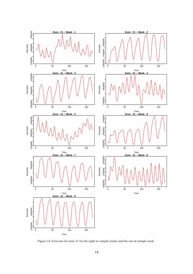
Zone : 21 − Week : 1
Time
fore
cast
s
0 50 100 150
1200
000
1800
000
2400
000 Zone : 21 − Week : 2
Time
fore
cast
s
0 50 100 1501000
000
1400
000
1800
000
Zone : 21 − Week : 3
Time
fore
cast
s
0 50 100 1501000
000
1600
000
2200
000 Zone : 21 − Week : 4
Time
fore
cast
s
0 50 100 150
1400
000
1800
000
Zone : 21 − Week : 5
Time
fore
cast
s
0 50 100 1501200
000
1800
000
2400
000
Zone : 21 − Week : 6
Time
fore
cast
s
0 50 100 1501000
000
1600
000
2200
000
Zone : 21 − Week : 7
Time
fore
cast
s
0 50 100 150
1500
000
2500
000
Zone : 21 − Week : 8
Time
fore
cast
s
0 50 100 150
1400
000
1700
000
2000
000
Zone : 21 − Week : 9
Time
fore
cast
s
0 50 100 1501200
000
1800
000
Figure 14: Forecasts for zone 21 for the eight in-sample weeks and the out-of-sample week.
18

Second, we used different models including different effects for each hour of the day to model thedemand patterns which are changing throughout the day.
Third, each hourly model allowed nonlinear and nonparametric terms to be included in the finalmodel. This provided a great flexibility to the model and avoided making too many assumptionsabout the data generating process.
Finally, gradient boosting has proven many times to be an effective prediction algorithm for bothclassification and regression tasks. By selecting the number of components included in the model,we can easily control the so-called bias-variance trade-off in the estimation. In addition, component-wise gradient boosting increases the attractiveness of boosting by adding automatic variable selectionduring the fitting process.
The Kaggle load forecasting competition was a challenging prediction task which required solv-ing several statistical problems such as data cleaning, variable selection, regression and multi-steptime series forecasting.
References
Buhlmann, P. (2006), ‘Boosting for high-dimensional linear models’, Annals of Statistics 34(2), 559–583.Buhlmann, P. and Hothorn, T. (2007), ‘Boosting algorithms: Regularization, prediction and model fitting’, Statistical Science
22(4), 477–505.Buhlmann, P. and Yu, B. (2003), ‘Boosting With the L2 Loss: Regression and Classification’, Journal of the American Statis-
tical Association 98, 324–339.Eilers, P. H. C. and Marx, B. D. (1996), ‘Flexible smoothing with B -splines and penalties’, Statistical Science 11(2), 89–121.Fan, S. and Chen, L. (2006), ‘Short-Term Load Forecasting Based on an Adaptive Hybrid Method’, IEEE Transactions on
Power Systems 21(1), 392–401.Fan, S. and Hyndman, R. J. (2012), ‘Short-term load forecasting based on a semi-parametric additive model’, IEEE Trans-
actions on Power Systems 27(1), 134–141.Fay, D., Ringwood, J. V., Condon, M. and Kelly, M. (2003), ‘24-h electrical load dataa sequential or partitioned time series?’,
Neurocomputing 55(3-4), 469–498.Freund, Y. (1995), ‘Boosting a weak learning algorithm by majority’, Information and computation pp. 1–50.Freund, Y. and Schapire, R. R. E. (1996), Experiments with a New Boosting Algorithm, in ‘Proceedings of the Thirteenth
International Conference on Machine Learning’, pp. 148–156.Friedman, J. H. (2001), ‘Greedy function approximation: A gradient boosting machine.’, Annals of Statistics 29(5), 1189–
1232.Friedman, J. and Hastie, T. (2000), ‘Additive logistic regression: a statistical view of boosting (With discussion and a
rejoinder by the authors)’, Annals of Statistics 28(2), 337–407.Hastie, T. J. and Tibshirani, R. (1995), Generalized additive models, Chapman & Hall/CRC, London.Hong, T., Pinson, P. and Fan, S. (2013), ‘Global Energy Forecasting Competition 2012’, International Journal of Forecasting
29. this issue.Hothorn, T., Buhlmann, P., Kneib, T., Schmid, M. and Hofner, B. (2012), mboost: Model-based boosting. R package version
2.1–3.McSharry, P. E., Bouwman, S. and Bloemhof, G. (2005), ‘Probabilistic forecasts of the magnitude and timing of peak
electricity demand’, IEEE Transactions on Power Systems 20, 1166–1172.Mease, D. (2008), ‘Evidence Contrary to the Statistical View of Boosting : A Rejoinder to Responses’, Journal of Machine
Learning Research 9, 195–201.Mease, D. and Wyner, A. (2008), ‘Evidence contrary to the statistical view of boosting’, The Journal of Machine Learning
Research 9, 131–156.Ramanathan, R., Engle, R. F., Granger, C. W. J., Vahid, F. and Brace, C. (1997), ‘Short-run forecasts of electricity loads and
peaks’, International Journal of Forecasting 13, 161–174.Schapire, R. (1990), ‘The strength of weak learnability’, Machine learning 5(2), 197–227.Schapire, R. E. and Freund, Y. (2012), Boosting: Foundations and Algorithms, The MIT Press.Schapire, R. E., Freund, Y., Bartlett, P. and Lee, W. S. (1998), ‘Boosting the margin: a new explanation for the effectiveness
of voting methods’, Annals of Statistics 26(5), 1651–1686.
19