DEPARTMENT OF ECONOMICS AND SOCIETY

D THESIS 2006

A GRAVITY MODEL FOR TRADE BETWEEN VIETNAM AND TWENTY-THREE EUROPEAN

COUNTRIES

Supervisor: Reza Mortazavi Author : Thai Tri Do

Abstract

This thesis examines the bilateral trade between Vietnam and twenty three European

countries based on a gravity model and panel data for years 1993 to 2004. Estimates

indicate that economic size, market size and real exchange rate of Vietnam and twenty

three European countries play major role in bilateral trade between Vietnam and these

countries. Distance and history, however, do not seem to drive the bilateral trade. The

results of gravity model are also applied to calculate the trade potential between Vietnam

and twenty three European countries. It shows that Vietnam’s trade with twenty three

European countries has considerable room for growth. Key words: Gravity model, panel data, trade potential, European countries, Vietnam.

Table of Contents

1. Introduction ............................................................................................................................ 1

2. Vietnam’s foreign trade overview.......................................................................................... 2

3. Trade with European countries in OECD .............................................................................. 5

4. Theory and Literature review................................................................................................. 6

4.1 Absolute and comparative advantage............................................................................... 7 4.2 Hecksher-Ohlin model ..................................................................................................... 7 4.3 New trade theory .............................................................................................................. 8 4.4 Gravity model................................................................................................................... 9

5. Empirical analysis ................................................................................................................ 12

5.1 Model ............................................................................................................................. 12 5.2 Data ................................................................................................................................ 12 5.3 Estimation Issues............................................................................................................ 14 5.4 Estimation results ........................................................................................................... 17 5.5 Trade potential................................................................................................................ 20

6. Conclusion:........................................................................................................................... 22

References ................................................................................................................................ 24

Appendix .....................................................................................................................................I

Table A1: Top export partners of Vietnam and their shares in total exports. .........................I Table A2: Top import partners of Vietnam and their shares in total imports . .......................I Table A3: Vietnam’s trade balance and growth rate of imports, exports ............................. II Table A4: Export by sector ................................................................................................... II Table A5: Import by sector .................................................................................................. III Table A6: Bilateral trade between Vietnam and EC23 and growth rate.............................. III TableA7: Total trade between Vietnam and EC23 in 2004, rank by country ...................... IV F test ..................................................................................................................................... IV Hausman test ......................................................................................................................... V

1. Introduction

European countries have always been Vietnam’s main trading partners. Before Vietnam

opened its economy and especially before the collapse of Council of Mutual Economic

Assistance (CMEA), Eastern European countries were dominant Vietnam’s foreign trade.

After Vietnam’s economic renovation, Western European countries take turn to play an

important role in Vietnam’s trade. European countries are now number one destination of

Vietnam’s exports and also one of top places of Vietnam’s imports.

Despite the important role of European countries, the empirical literature analysing

Vietnam’s trade with European countries is still rather limited. Thus, it is interesting to

investigate the trade between Vietnam and European countries in depth. This paper applies

the gravity model to investigate the bilateral trade between Vietnam and twenty three

European countries (EC23) in Organization for Economic Co-operation and Development

(OECD) namely: Austria, Belgium, Czech Republic, Denmark, Finland, France, Germany,

Greece, Hungary, Iceland, Ireland, Italy, Luxembourg, Netherlands, Norway, Poland,

Portugal, Slovak Republic, Sweden, Switzerland, Turkey, United Kingdom over twelve

years period from 1993 to 2004. The purpose of the paper is two-folds: to identify

significant factors influencing the levels of trade between Vietnam and EC23, and to test

whether trade between Vietnam and EC23 fully exploits their potentials or there is still

room for more trade. The findings of this paper may be served as recommendations for

policy makers to improve the bilateral trade between Vietnam and EC23, one of its main

trading partners.

Gravity model has been used intensively in literature to investigate bilateral trade.

Blomqvist (2004), for example, applies gravity model to explain the trade flow of

Singapore. Montanari (2005) investigates the European Union (EU) trade with Balkans by

applying a gravity model. Countries in Association of South East Asia Nations (ASEAN)

have also been included in a number of studies used gravity approach such as Anaman and

Al-Kharusa (2003) for Brunei’s trade with EU, Thornton and Goglio(2002) for intra-trade

in ASEAN. However, it appears that there are a limited number of studies applying gravity

1

model for the case of Vietnam. Moreover, it seems that there has not been any study of

bilateral trade between Vietnam and European countries in a gravity model framework.

This paper tries to fill the gaps in literature concerning Vietnam and European countries by

utilizing gravity model to explore the relationship between Vietnam and EC23 for years

1993 to 2004. The gravity model estimated in this paper is based on panel data with

pooled, random and fixed effect estimation and allowing for proper representation of

individual country effects and business cycle (time effects). The estimated results of

gravity model are then used to calculate the trade potential between Vietnam and EC23 by

applying method of speech of convergence.

The remainder of the paper is structured as follows: Section 2 provides an overview of

Vietnam’s foreign trade. The analysis of Vietnam and EC23 bilateral trade is given in

Section 3. Section 4 presents a brief theory of international trade and literature review of

gravity model. Section 5 applies the gravity model to analyse the trade flow and calculate

the trade potential between Vietnam and EC23. Section 6 concludes the paper.

2. Vietnam’s foreign trade overview

After country reunification in 1975, Vietnam’s trade was almost exclusively with the

Soviet Union and the other countries of the Council of Mutual Economic Assistance

(CMEA). The Soviet dominated trading arrangement with most of socialist countries

included Vietnam. Under this arrangement, Vietnam imported Soviet oil, food at low

prices, which were financed by Vietnam’s exports of rubber, consumer commodities to

CMEA and preferential loans mainly from the Soviet Union. With Soviet’s subsidies,

Vietnam can supply food and bare necessities for its people, but not fully enough.

Vietnam’s economy was unstable and heavily depended on imported goods and aids from

outside. The central planning system of socialist and international isolation added even

more difficulties for the economy. As a result, Vietnam had fallen into severe

macroeconomic crises even before the collapse of CMEA in 1990. Inflation rate reached

level of over 600 percent by 1986, import was 4 to 5 times greater than export, and there

were serious shortage of food and essential consumer goods like clothes and medicine

(Vietnam consulate, 2005)

2

In late of 1986, Vietnam implemented the far-reaching reform to open itself to the world,

known as “doi moi”. The essential component of “doi moi” has been changes in trade

policies with price liberalization, exchange rate unification, tax reform, and modernization

of the financial system. In addition, small and medium enterprises are allowed to do import

and export activities breaking the monopoly of the state-owned enterprise. These reforms

have led to rapid export and import growth. As can be seen in table 1 export sector has

expanded by over 300 percent; import has increased over 100 percent during the transition

period 1986-1993.

Table1: Increase in trade

Million US dollar 1985 1993 Percentage increase

Value of export 698,5 2985,2 327%

Value of import 1857,4 3924,0 111%

Source: Vietnam general statistic office 2005

The trade reorientation is perhaps the most important change on Vietnam’s trade pattern.

As the CMEA began to fall apart in 1989 and by 1991 with the collapse of Soviet Union,

Vietnam’s trade contracted by about two-third. In response, Vietnam insisted on trade

liberalization as well as looked for new trading partners for its traditional exports. The

correct response yielded good results; Vietnam has gradually built up trade relationships

with hundreds of countries all over the world. Almost all of Vietnam’s top trading partners

nowadays are from countries outside the previous CMEA.

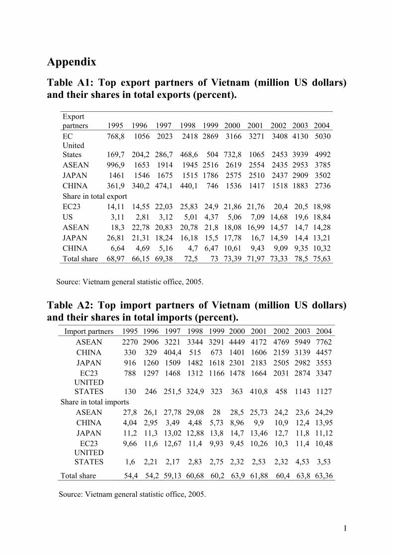
Table A1 (in appendix) shows Vietnam’s top export partners. European countries were the

top destinations for Vietnam exports, with total value of over 5 billion US dollar,

accounting for about 18,9% of total exports in 2004. The top position of EC23 had

remained stable for years since the late 1990s, followed by United States (18,8%),

ASEAN(14,28%), Japan(13,2%), and China(10,3%). These partners absorbed over 75

percent of Vietnam’s total exports in 2004.

In imports, ASEAN was Vietnam’s number 1 partner, accounting for 24,2% of total

imports in 2004, followed by China (13,9%), and Japan (11,1%). Imports from EC23 and

United States had increased in recent years; EC23 (10,4%) and United States (3,5%) were

3

the fourth and fifth leading exporters of Vietnam. All these partners accounted for over

sixty percent of Vietnam’s imports in 2004 (table A2, appendix).

Over two decades after opening its door, Vietnam’s foreign trade has performed

impressively, with exports grew at average of 19,72 percent per year from 1995 to 2004. In

2004 growing rate of exports was 31,54 percent (against 20,61 percent in 2003) reaching

US dollar 26,5 billion (table A3 in appendix). However, from the structural point of view,

the export base is highly narrow. Vietnam enjoys an uneven export structure, dominated by

almost two groups of commodities crude oil and textiles and garments, accounting for

nearly 40 percent of total exports (see table A4 in appendix). Therefore, Vietnam exports

are very sensitive to change in market condition.

Imports rose by a robust of 17.23% annually from 1995 to 2004, in 2004 imports were US

dollar 31.9 billion, increasing 26 % in comparison with imports’ value in 2003. Imports

and exports rise nearly at the same rate; however the absolute value of imports is much

bigger than that of exports. As a result, Vietnam exhibits deficit in trade for a long time.

The trade deficit has tendency to increase in recent years and reached an all-time record of

US dollar 5.4 billion in 2004, nearly 4% of GDP (table A3 in appendix).

A significant part of the trade deficit can be related to robust domestic investment as well

as imports needed as inputs for export production. Three largest imports were in machinery

and equipment, petroleum products and material for textiles and footwear. The three

sectors together accounted for nearly 40% in 2003 and 35% in 2004 of total imports (table

A5, appendix). The deficit seems to be obvious for Vietnam as a developing country with

investment driven export, yet it also flags a weakness of Vietnam economy that is heavily

depended on imports for inputs needed for key export industries such as textiles and

garments and footwear. Vietnam just gets small profit from processing based on cheap

labour forces.

4

3. Trade with European countries in OECD

After the country’s independent in 1975, trade between Vietnam and EC23 was influenced

by the same factors that affected Vietnam’s foreign trade such as international isolation

and trade concentration with CMEA. Vietnam traded intensively with communist countries

in EC23 such as Poland, Hungary; however trade with other non-communist countries in

EC23 was quite limited, just in form of aids and barter trade regime (Lawrence and Jenelle,

1985). After Vietnam opened its economy and ended its connection with countries in

Council of Mutual Economic Assistance, bilateral trade between Vietnam and EC23 was

liberalized and increased substantially.

Over the period 1995-2004 Vietnam’s trade with EC23 grew faster than Vietnam’s trade

with the world. Vietnam’s exports to EC23 increased 25,33 percent a year on average,

while its imports from EC23 grew at 19,49 percent, which were considerably faster than

the growth of Vietnam’s overall export and import (19,72 and 17,23 percent) ( table 3 and

table 6, appendix). EC23 has become number one destination for Vietnam exports since

the late 1990s and ranked fourth in Vietnam’s top import partners.

Vietnam trades unequally with individual countries in EC23, most of growth in bilateral

trade between Vietnam and EC23 can be attributed to the increasing in trade between

Vietnam and Germany, United Kingdom, France. The three big economies are leading in

trade with Vietnam, each country’s total trade exceeds 1.4 billion US dollar in 2004. Italy,

Netherlands and Spain are next big partners with total trade of over 500 million US dollars

per country. Small country likes Luxembourg is among countries that have little trade with

Vietnam with total trade less than 10 million US Dollars (table A7, appendix).

There is an interesting situation in bilateral trade between Vietnam and EC23. As

mentioned earlier, Vietnam has trade deficit with the world because imports are much

higher than exports, Vietnam, however, has enjoyed trade surplus with EC23 for many

years. As can be seen from figure 1, trade surplus has been over one billion US dollars per

year since 1997 and reached the highest peak, five billion US dollars in 2004.

5

0

1000

2000

3000

4000

5000

6000

7000

8000

9000

0

1000

2000

3000

4000

5000

6000

7000

8000

9000

Export 771,48 1262,4 1799,9 2276,5 3221,2 3810,7 4496,9 4973 5102,7 5652,3 7012,8 8167,8

Import 682,72 921,68 1163,6 1820,8 1592 1384,6 1340,3 1418,4 1731,9 1988,7 2783 2857,3

Balance of Trade 88,76 340,71 636,32 455,66 1629,3 2426,1 3156,6 3554,6 3370,7 3663,6 4229,8 5310,4

1993 1994 1995 1996 1997 1998 1999 2000 2001 2002 2003 2004

Figure 1: Trade balance between Vietnam and EC23 (million US dollars)

Source: OECD

This trade pattern raises the question whether the integration of Vietnam with these

economies has reached an advanced stage? Is there any economy in EC23 that may have

more integration with Vietnam? These questions will be answered quantitatively on the

basis of a gravity model in the empirical analysis section.

4. Theory and Literature review

Nowadays, countries are more closely linked through trade. Developed and developing

countries are lifting their trade barriers to invite more trade from others. The words like

free trade, trade liberalization are often mentioned in public’s news. Why do countries

trade with each other? Do all countries benefit from trade? How large are their trade flows?

To understand these questions thoroughly, it is a good idea to look for answer in the trade

theory. In the following part, I will introduce some theories of international trade such as

the classical trade theory, new trade theory and the gravity model. A brief introduction of

classical and new trade theory will explain the “why” behind trading reasons, while gravity

model will answer the question of the magnitude of trade between countries, which cannot

be explained by other theories of international trade.

6

4.1 Absolute and comparative advantage

The first, which is considered the father of trade theory, is absolute advantage theory by

Adam Smith. In his famous book The Wealth of Nation, Adam Smith compared nations to

households. The tailor makes a shirt then exchanges it for a shoe with the shoe-maker, thus

both of them gain and the same should apply to nations. Countries specialize in the

production of goods according to their absolute advantage, then trade with others, they all

gain in international trade (see also Lindert, 1991). Smith’s argument is convincing,

however, only for country which has absolute advantage, it cannot explain the reason for a

country which does not have absolute advantage to attend international trade.

David Ricardo answered questions left by Adam Smith satisfactorily and established a

fundamental theory of international trade, known as the principle of comparative

advantage. The principle states that “ a nation, like a person, gains from trade by exporting

the goods or services in which it has its greatest comparative advantage in productivity and

importing those in which it has the least comparative advantage” ( Lindert, 1991).

Comparative advantage and comparative disadvantage as explained by Ricardian model

mean that the opportunity cost of producing the good is lower or higher at one country than

in the other country.

It is clear that comparative advantage is a basis for international trade. However the

Ricardian model is still incomplete in many ways. First, the model assumes an extreme

degree of specialization, which is unrealistic because Sweden, for example, imports and

produces machinery at the same time. Second, it predicts that every country gains from

trade because it does not take into consideration the effects of international trade on

income distribution within countries. Third, different resources among countries, role of

economies of scale, intra industry trade are absent in Ricardian model.

4.2 Hecksher-Ohlin model

The classical theory has several defects, which are the motivation for economists of

nineteenth and twentieth centuries to modify. Two Swedish economists Eli Hecksher and

Bertil Ohlin had extended the Ricardian model and developed an influential theory of trade,

known as factor endowment theory or Hecksher-Ohlin model. The model predicts that

7

“countries export products that use their abundant factors intensively and import the

products using scarce factors intensively” (Lindert, 1991)

The Hecksher-Ohlin (H-O) model had modified the simple Ricadian model in that it added

one more factor of production, capital, beside labour, the original factor in the classical

model. The H-O model also assumes that the only difference between countries is the

differences in the relative endowments of factors of production, the production

technologies are the same, whereas the Ricardian model assumes that production

technologies differ between countries. The assumption of same technology is to see what

impacts on trade will arise due to difference proportion in factors of production in

difference countries.

In H-O model, trade generally does not lead to complete specialization between countries;

this can overcome the defect in Ricardian model which argues that trade leads to complete

specification. Another argument that separates H-O model from Ricardian model is that

not every country gains from trade; international trade has strong income distribution

effects. The owners of the country’s abundant factors gain from trade while the owners of

scarce factors lose (see Husted and Melvin, 2001).

4.3 New trade theory

The classical trade theory implies that countries which are less similar tend to trade more.

Therefore it is unable to explain the huge proportion of trade between nations with similar

factor of endowments and intra industrial trade which dominate the trade of developed

economies. This is the motivation for new trade theory which has been established in the

1980s by researchers like Krugman, Lancaster, Helpman, Markusen, and many others.

New trade theory explains the world trade based on the economic of scale, imperfect

competition and product differentiation which relax the strict assumptions of classical

theory of constant return to scale, perfect competition and homogeneous goods. Under

these assumptions each country can specialize in producing a narrower range of products at

larger scale with higher productivity and lower costs. Then it can increase the variety of

goods available to its consumers through trade. Trade occurs even when countries do not

differ in their resources or technology (see also Markusen et al, 1995; Krugman and

Maurice, 2005).

8

4.4 Gravity model

The classical and new trade theory can successfully explain the reasons for countries to

join in world trade; however they can not answer the question of the size of the trade flows.

Another trade theory, the gravity model, which has been used intensively in analysing

patterns and performances of international trade in recent years, can be applied to quantify

the trade flows empirically. The model applies Newton’s universal law of gravitation in

physics, which states that the gravitational attraction between two objects is proportional of

their masses and inversely relate to square of their distance. The gravity model is expressed

as follows:

2ij

ji

D

MMFij = (1)

Where:

Fij is the gravitational attraction

Mi, Mj are the mass of two objects

Dij is the distance

Tinbergen was first applied this gravity model to analyse international trade flows in 1962

and many others had followed to set up a series of econometric model of bilateral trade

flows. The general gravity model applied in bilateral trade has the following form (see also

Krugman and Maurice, 2005):

ij

jiij D

YYAT = (2)

Where

A is a constant term

Tij is the total trade flow from origin country i to destination country j

Yi, Yj are the economic size of two country i and j. Yi, Yj are usually gross domestic

product (GDP) or gross national product (GNP).

Dij is the distance between two country i and j.

9

The gravity model has long been criticized for being ad hoc and lacking of theoretical

foundation. Therefore in recent years there has been increasing interest in providing the

theoretical support for the gravity model. Linneman (1966) (cited in Radman, 2003) is

perhaps the first author who provided theoretical background for gravity model; he showed

that the gravity equation could be derived from a partial equilibrium model. Trade flows

between two countries i and j are explained by factors that indicate total potential supply of

country i, total potential demand of country j, and the resistance factors to trade flow

between i and j. The gravity model is then obtained by equality of supply and demand.

Bergstrand (1985), however, criticizes this approach for inability to explain the

multiplicative functional form of the gravity equation and claims that the gravity equation

may be misspecified due omitting price variable. Bergstrand used a microeconomic

foundation to explain the gravity model. The country trade supply is derived from firms

profit maximization and trade demand is derived by maximizing the constant elasticity of

substitution utility function subject to income constraint. Then gravity equation is obtained

by using market equilibrium clearance.

Other authors, on the other hand, attempted to derive gravity model from theories of

international trade. Eaton and Kortum (1997) developed a Ricardian model and showed

that gravity equation could be obtain from a Ricardian framework but identified underlying

parameters of technology. While Deardorff (1998) proved that gravity model could arise

from two extreme cases of Hecksher-Ohlin model with and without trade impediments.

Gravity model has been extremely successful empirically. Models of this type have now

been estimated for a wide range of countries. Radman (2003) uses import export and total

trade, three equations to investigate trade flow between Bangladesh and its major trading

partners. He finds that Bangladesh’s trade in general is determined by the size of the

economy, GNP per capita, distance and openness. Blomqvist (2004) applies gravity model

to explain the trade flow of Singapore and as usual with gravity model, a very high degree

of explanation is achieved especially for the GDP and distance variable. Anaman and Al-

Kharusa (2003) on the other hand show that in a gravity model framework, the determinant

of Brunei’s trade with EU is mainly from the population of Brunei and EU countries.

10

Gravity model is also applied to explain the trade relationship between trade blocs and

intra trade of economic blocs. Using gravity model Tang (2003) finds that EU integration

has resulted in significant trade decrease with ASEAN, NAFTA (North American Free

Trade Agreement) during period 1981- 2000. Thornton and Goglio (2002) prove the

important of economic size, geography distance and common language in intra regional

bilateral trade for ASEAN

Martinez-Zarzoso et al (2004) classify export sectors according to their sensitivity to

geographical and economic distance and under gravity model framework they can identify

which commodities enjoy export strength. Their results show that sectors such as footwear,

furniture enjoy high and significant geographical effect in bilateral trading between EU and

countries in Southern Common Market (comprising Argentina, Paraguay, Uruguay and

Brazil).

There are a huge number of empirical applications of gravity model; it is not strange to

have many variations of gravity equation. However, within that intensive literature gravity

model also shares some common features. First, gravity model is applied to explain

bilateral trade, the dependent variable of the gravity equation is always trade variable.

Second, economics mass of exporting and importing country are measured by GDP, GNP

or GNP per capita ,GDP per capita in some augmenting gravity model such as Radman (

2003), Montanari (2005). The idea behind this is countries with higher income tend to

trade more and those with lower income trade less.

Third, distance is another commonly used variable in gravity model. Distance is the

geographical distance between countries; it is also a proxy for transport cost, which is

usually measured as the straight-line distance between the countries’ economic centers

(usually capitals). However it is not very accurate measure in some cases such as using

Beijing, capital of China maybe under or over estimate the distance between China and

other trading partners because China has many economic centers that are thousand

kilometres apart. Finally, dummy variables are always included in gravity equation in order

to investigate the qualitative variables such as border, languages, colonial history, and

trade agreement in bilateral trade.

11

5. Empirical analysis

5.1 Model

Among the above mentioned trade theories, the gravity model will be chosen to quantify

the Vietnam’s trade with its twenty-three European countries’ trading partners. The model

applied in this paper is a variation of the gravity model given by Krugman and Maurice

(2005). The model is augmented first by adding a financial variable, exchange rate, which

acts as a proxy for price, then by including history and population of original and target

countries as additional mass for bilateral trade. The estimated gravity model has the

following form:

Log(Tijt) = α0 +α1log(YitYjt)+α2log(NitNjt)+ α3Erijt +α 4logDij+α5His +eijt (3)

Where:

j= 1, 2,…,23.

i=1 (Vietnam).

t=1993, 1994,…, 2004.

Tijt : Vietnam’s trade with country j in year t.

Yit : Vietnam GDP in year t.

Yjt : Country j GDP in year t.

Nit : Population of Vietnam in year t.

Njt : Population of country j in year t.

Erijt: Real exchange rate between Vietnam and country j in year t.

Dij: Distance in kilometres between Vietnam and country j.

His: History dummy variable.

eijt: Error term.

5.2 Data

Data set contains annual trade flows, GDPs, population, exchange rate and distance of

Vietnam and twenty three countries in European countries (EC23) in Organization for

Economic Co-operation and Development (OECD) namely: Austria, Belgium, Czech

Republic, Denmark, Finland, France, Germany, Greece, Hungary, Iceland, Ireland, Italy,

12

Luxembourg, Netherlands, Norway, Poland, Portugal, Slovak Republic, Sweden,

Switzerland, Turkey, United Kingdom for the time period from 1993 to 2004. Annual trade

(imports plus exports) is calculated as average of monthly figures which are taken from

OECD data base. The product of GDP of Vietnam and EC23 in time t is used as a measure

of economic size. This variable is expected to be positively and significantly related to

trade. Gross domestic product of EC23 and Vietnam are obtained from international

monetary fund (IMF), both of them are in US current dollars and converted into constant

US price of 1996 using the GDP deflator given by IMF. Population is included in the set of

variables inform of product of both parties’ population with the intention to estimate the

market size, another dimension to the concept “country mass”. The larger the market the

more it trades; therefore, market size is expected to turn out with positive sign. Data of

EC23’s population are obtained from OECD source, while those of Vietnam are from the

World Bank.

Empirical studies have shown that exchange rate in addition to gravity equation is

significant in explaining trade variations among participating countries, see Bergstrand

(1985), Dell’Ariccia (1999). Therefore, exchange rate will be included as an explanatory

variable in the model. The nominal exchange rate is calculated as the annual average of the

national currency unit of EC23 per US dollar divided by the annual average of the national

currency unit of Vietnam per US dollar. The nominal exchange rate is then multiplied by

EC23’s GDP deflator and divided by Vietnam’s GDP deflator to get the real exchange rate.

Data of exchange rate for both EC23 and Vietnam are obtained from Penn World data and

supplemented by those from Federal Reserve Bank of New York and Vietnam commercial

bank.

The effect of real exchange rate variable on bilateral trade between Vietnam and EC23 is

expected to be negative. Vietnam’s currency appreciation is represented by a rise in real

exchange rate, as a result exports would be more expensive and imports would be cheaper.

It seems reasonable to assume that the former effect will dominate in bilateral trade

between Vietnam and EC23, or an increase in real exchange rate will lead to a decrease in

bilateral trade. It is because Vietnam has had trade surplus with EC23 for many years and

most of Vietnam’s exports are labour-intensive products, while imports are capital-

intensive products, therefore exports are more sensitive to fluctuation in market price.

13

Distance is involved in the analysis as proxy for transportation cost between Vietnam and

EC23; it is calculated by distance in kilometres between Hanoi, capital of Vietnam, and the

capital city of countries in EC23. Data on distance are taken from great circle distance

between capital cities (Byers, 1997) where distance is measured as the minimum distance

along the surface of the earth. This variable is expected to have negative effect to trade as

transport cost increase with the distance between countries. The last variable is history,

which comes inform of a dummy variable, representing EC23 members with colonial ties

to Vietnam. A value of 1 denotes France and zero is for the remaining members. History is

expected to have positive sign.

5.3 Estimation Issues

A panel framework is designed to cover trade variation between Vietnam and its twenty-

three trading partners during a period of twelve years. Panel estimation reveals several

advantages over cross section data and time series data as it controls for individual

heterogeneity, time series and cross section studies do not control for this heterogeneity

may give biased estimated results. Panel data offer more variability, more degree of

freedom and reduce the collinearity among explanatory variables therefore improving the

efficiency of the econometric estimates. More importantly, panel data can measure effects

that are not detectable in cross sections and time series data. (see Baltagi, 1995).

Some early studies usually investigate the gravity model with single-year cross-sectional

data or time series data. These methods are probably affected by problem of

misspecification and yield biased estimates of volume of bilateral trade because there is no

controlling for heterogeneity (see Cheng and Wall 2005). Egger (2000), Matyas et al

(1997) suggest applying panel data in gravity model, because panel data is a general case

of cross-sectional data and time series data. According to Matyas et al (1997), the most

natural representation of bilateral trade flows with gravity equation is a three-way

specification, which is expressed as:

y= DNα+DJγ+DTλ+Zβ+ε (4)

Where

y is vector of dependent variable

14

Z is the matrix of explanatory variables

DN, DJ, DT are dummy variable matrics

α is local country effect

γ: target country effect

λ is time effect

β is parameter vector of explanatory variables.

ε is error term

When the cross section data is used with one specific year it means there are no time

effects, λ =0, when time series is used it can just cover effect for specific pair of countries

which implies α= γ=0. When panel data is used there is no such necessary restriction, it can

take into account both country and time effects at the same time.

Panel estimation can be done using pool estimation, fixed effect and random effect

(Gujarati, 2003). Pool estimation is the simplest approach; its function is as follow:

Yit = β1+ β2X2it+ β3X3it +εit (5)

Where i stands for cross sectional unit, t stands for time period and error term is normally

distributed with mean zero and constant variance. Pooled estimation assumes there is one

single set of slope coefficients and one overall intercept. It disregards the time and space

dimension of panel data; the error term captures the difference over time and individuals.

The pooled estimation, however, may provide inefficient and biased estimated results

because it assumes there are no individual effects and time effects.

The fixed effect takes into account the individual and time effects by letting the intercept

varies for each individual and time period, but the slope coefficients are constant, the

model is:

Yit = β1i+ β2X2it+ β3X3it +εit (6)

Where it is usually assumed that ε is independent and identically distributed over

individuals and time with mean zero and variance σ2, and all Xit are independent of all

15

error terms. By introducing different intercept dummies we can allow for intercept vary

according to individuals and time.

One of the shortcomings of fixed effect model is that it may not be able to identify the

impact of time invariant such as distance, and this variable will be excluded from

estimation. To overcome this problem, some papers use random effect or Hausman and

Taylor’s estimator. Cheng and Wall (2005) has suggested a method to estimate the time

invariant variables by using the individual effects. In the fixed effect model the country

pair individual effects cover all factors that remain constant over time such as: location,

language, culture, and other trade barriers. Therefore, we can indirectly calculate the effect

of time invariant variables like history and distance from the individual effects. I first

estimate the model using the fixed effect estimator, then follow Cheng and Wall (2005) to

estimate an additional regression of the estimated country pair effects on the time invariant

variables in order to find out the importance of these variables in the fixed effects. The

regression is as follows:

αij = a1 + a2dij+ a3his +eij (7)

Where:

αij is country individual effects

a1,a2,a3 are coefficients.

dij is distance between Vietnam and EC23

his is history dummy variable and eij is error term.

Another approach applies to estimate panel data is random effect estimation. The random

effect treats the intercept as a random variable and the individuals included in the sample

are drawn from a larger population. The model is written as follows

Yit = β1+ β2X2it+ β3X3it +wit (8)

Where: wit= εi +uit

It is assumed that the individual error components are not correlated with each other and

are not auto correlated across both cross section and time series units.

16

εi ~ N (0, σ2ε)

uit ~ N (0, σ2u)

E(εi,uit) = 0, E(εi,ε j) = 0 (i ≠ j)

E(uit,uis) = E(uit,ujt) = E(uit,ujs) = 0 (i ≠ j, t ≠ s)

Empirical work on applying gravity model does not give a clear answer on which

estimation method pooled estimation, random or fixed effect does give more efficient

results. Therefore, first, trade equation will be estimated by all three methods, then F

statistic test and Hausman test (Verbeek, 2004) will be run to select the most efficient

method for interpreting the estimate results.

5.4 Estimation results

The estimation results of bilateral trade between Vietnam and EC23 using equation (3) are

given in table 2. The first column shows the results following the fixed effect method

which is suggested by Cheng and Wall (2005). Results from pooled estimation and random

effect method are reported in column two and three.

Table2: Estimated results

Fixed effect Pool estimation Random effect Coefficient P-value Coefficient P-value Coefficient P-value YiYjt 0,2927 0,043913 0,9174876 1,408E-25 1,1666777 4,6379E-10NiNj 7,93552 9,88E-44 0,22417611 0,0029757 0,260352 0,15418861Erij -0,0322 0,030717 -0,09672163 7,989E-11 -0,106483 1,7737E-07Dij 21,8125 0,385239 -2,0481802 0,0002475 -2,021083 0,29058785His -13,911 0,218097 0,36028625 0,1284339 -0,270854 0,74258824

Trade’s equation runs through three estimation methods shows to be consistent, estimated

coefficients have nearly all the expected signs, except for distance and history variable.

However, the magnitudes of the coefficients in pooled and random effect estimation are

notably different from those in the fixed effect method suggesting that there may be bias

17

results due to ignoring country individual effects in pooled estimation and inconsistent

estimates because of correlation between the individual effects and other regressors in

random effect method.

Formally, an F test has been carried out to test for the null hypothesis that the country-

specific effects are jointly zero (see appendix VIII). The result of F test clearly rejects the

null hypothesis, which indicates that countries in EC23 have different propensities to trade

with Vietnam, and the pooled estimation gives biased results due to omitted variables.

Next, the Hausman test (see appendix IX) is performed to compare the fixed and random

effect estimators. The statistic result takes a value of 136,46 which is far larger than the

critical value with three degrees of freedom. This suggests that the fixed effect is a better

choice than random effect. The direction of my analytical efforts then focuses on the fixed

effects estimation

The determinants of bilateral trade between Vietnam and EC23 are: economic size, market

size and the real exchange rate volatility. Distance and history seem to have no effect on

bilateral trade between Vietnam and EC23, as they are statistically insignificant. Economic

size variable results to be significantly positive related to trade volume, showing that

Vietnam tends to trade more with larger economies. An increase by 1% of product of

Vietnam’s GDP and EC23’s GDP will go in increasing bilateral trade between them by an

average index of 0.29%. Market size of Vietnam and EC23 have significant and strong

effect on trade, market size increases by 1% the bilateral trade between Vietnam and EC23

will increase up to 7,9% on average. The estimate coefficient for real exchange rate is

significant and negative correlation with trade variation indicating that price

competitiveness is important for bilateral trade between Vietnam and EC23, 1 percent

depreciation of Vietnam’s currency will increase bilateral trade about 0,03%.

The finding of this paper is consistent with other empirical work in explaining bilateral

trade variation using gravity model. Economic size and market size have strong influence

on trade as larger country can produce more goods and services for export, high income

together with big market size will increase the demand for importing goods. The negative

coefficient of real exchange rate on bilateral trade is also in line with other papers such as

that of Dell’Aricaca (1999). However, it is interesting to note that the magnitude of the real

exchange rate coefficient is rather small of only 0,03, which suggests that fluctuation of

18

exchange rate of Vietnam currency has not well-supported trade activities in this period.

This weak impact can be explained by the effect of change in exchange rate on imports and

exports are cancelling each other. On the other hand, it also shows that Vietnam exchange

rate policy in recent years has not been efficient in increasing the export product

competitiveness.

The distance and history variables turn out with unexpected signs and insignificant, it may

be because there are still other unexplained variables besides the distance and history in the

second regression between these variables against the country individual effects. Another

reason for distance to be insignificant as suggested by Anaman and Al-kharusi (2003) can

be due to the geographical closeness of European countries.

Figure 2 plots the time effects of bilateral trade between Vietnam and EC23, these effects

are all individually significant. Vietnam’s trade with EC23 has increased substantially from

1993 to 2000. After 2000 until recently the bilateral trade, however, has tendency to

decrease.

-13

-12,5

-12

-11,5

-11

-10,51993 1994 1995 1996 1997 1998 1999 2000 2001 2002 2003 2004

Figure 2: Time effects of trade between Vietnam and EC23.

The recession can be explained from the impact of Asia financial crisis in 1998 had on

foreign invested companies in Vietnam slowing down trade. Another reason can be due to

the increasing trade between Vietnam and United States after year 2000 and rocketing in

the beginning of 2002 as the Vietnam and United States bilateral trade agreement came

19

into force. Vietnam’s exports to United States share a large portion of Vietnam’s exports to

EC23 especially in textiles and garments and footwear. However it is also needed to

mention the unattractive business environment such as high cost, bureaucracy which

companies face when doing business in Vietnam in recent years.

5.5 Trade potential

Calculating trade potential is a line of research that has been used intensively with the

gravity model, especially for Central and Eastern European countries, such as study of

Maurel and Cheikbossian (1998), Montanari (2005). They apply the point estimated

coefficients to data on the explanatory variables to calculate the trade potential predicted

by the gravity model. Then this trade potential will be compared with the actual trade to

see whether bilateral trade between two countries have been overused or underused.

Recent research has highlighted the white noise residuals when using this method to

calculate trade potential, for instance, Egger (2002) considers the underused or overused of

trade to be the signs for econometric misspecification. Taking into consideration the

criticisms about the uncertainty of calculating potential trade based on point estimates,

Jakab et al (2001) propose the concept of speed of convergence to replace the old method

to calculate potential trade. The average speed of convergence is defined as the average

growth rate of potential trade divided by average growth rate of actual trade between the

years of observation:

Speed of convergence = (Average growth rate of potential trade / average growth rate of

actual trade)*100-100. (9)

Accordingly, we posit convergence if growth rate of potential trade is lower than that of

actual trade and the computed speed of convergence is negative. We have the divergence

in the opposite case. The argument for the prominent efficiency of this method over the

point estimated method is that the speed of convergence exploits the dynamic structure of

the data during the estimation, which offers more reliable than the analysis of point

estimates. The convergence is proved to be quite robust with different methodologies such

as pool estimation, fixed effect, and random effect in Jakab et al’s paper.

20

In estimating the trade potential I use results obtained from regression of equation (3) with

fixed effects and apply the speed of convergence in equation (9) to calculate the potential

of trade between Vietnam and EC23. The speed of convergence is calculated as ratio of

average growth rate of potential trade and growth rate of actual trade over twelve years of

the study.

The results of potential trade are reported in table 3. Vietnam trade with EC23 presents an

interesting situation separating trade partners into two groups, the first group characterized

by an overtrade situation and the second one reflecting potentials to develop trade.

Vietnam has convergence in trade with 15 countries out of 23 countries in EC23 and

divergence with other eight countries. In other words, Vietnam has not exploited all the

potentials in trading with EC23. Trade between Vietnam and EC23 still has large room for

growth.

Table 3: Trade potential between Vietnam and EC23 using speech of convergence

Country Potential trade Country

Potential trade

Austria -2,5828 Ireland 59,2467 Belgium -5,4484 Iceland 4,2936 Switzerland -8,4396 Italy -20,3484 Czech Repuplic 7,4179 Luxembourg -21,3593 Germany -1,4852 Netherland -5,3045 Denmark -23,5418 Norway 114,0632 Spain 12,0000 Poland 71,5806 Finland -8,9728 Portugal -308,2565 France 1,1892 Slovak Republic -159,6890 United Kingdom -10,7447 Sweden -7,3474 Greece -26,7196 Turkey 248,6106 Hungary -54,7886

Some of the reasons that bring about the sorting situation are imports of Vietnam from

some of the big countries in EC23 such as Germany, United Kingdom, Italy and

Netherland are still small because of habit of Vietnamese to import from nearby countries

21

in the region and Vietnam may not have enough attractions for business men from those

countries. Tendency to do business with large economies as predicted by the gravity model

can also help to explain the presence of unutilized trade potentials between Vietnam and

other small countries such as Austria, Finland, Luxembourg.

For overtrade with France, the answer lies partly in cultural affinity. There are quite a lot of

Vietnamese immigrant to France, the investment of Vietnamese nationals and the money

transfer home help to increase trade between Vietnam and France. Trade with Poland and

Czech Republic may be overused due to previous trade connections between Vietnam and

these former socialist countries in CMEA. The increasing foreign direct investment can

help to explain the over-utilized trade potential between Vietnam and countries such as

Turkey, Ireland, Spain, and Norway.

6. Conclusion

The main purpose of this paper is to find out the factors influencing the level of trade

between Vietnam and twenty three European countries in OECD, and to evaluate whether

there are potentials for growth in trade between Vietnam and those countries. In this

respect, a gravity model has been estimated with panel data and pooled, random, fixed

effect estimation covering the period of twelve years from 1993 to 2004. The main results

indicate that the bilateral trade flows between Vietnam and EC23 are driven by economic

size, market size and exchange rate volatility. Distance and history, however, seem to have

no effect on bilateral trade between Vietnam and EC23. For most of countries in EC23,

trades with Vietnam are still under potential levels.

Bilateral trade between Vietnam and EC23 increases with economic size and market size

implies that economic growth of individual economies will strongly affect trade

relationship. Therefore stabilization policies and attractive business environment which

contribute to bring about the high growth rate for the country are important issues for

Vietnam’s policy makers.

Evidence of a small but significant negative effect of real exchange rate on bilateral trade

between Vietnam and EC23 confirms that exchange rate volatility does have impact on

trade; however, its contribution to trade is quite limited. Vietnam’s central bank should

22

manage the exchange rate movement more efficiently in order to boost trade between

Vietnam and EC23.

Although Vietnam has trade surplus with EC23 for years, Vietnam, in general, has

unrealized trade potentials with EC23. This finding is extremely important for policy-

maker because exploiting these trade potentials are expected to contribute to trade

diversification for Vietnam. It is suggested that Vietnam needs to sign bilateral trade

agreement with individual country in EC23; bilateral trade agreement such as the case of

Vietnam and United States trade agreement would increase trade substantially. Moreover,

besides trading with large countries in EC23, increasing trade with small economies which

have trade potentials such as Austria, Luxembourg would also be of priority.

Estimated results show that bilateral trade between Vietnam and EC23 has entered

recession for years. It is not because bilateral trade has reached its peak; it is, however,

mainly due to the unattractive business environment and the tendency to trade intensively

with new market. A more attractive business environment together with market

reorientation from government could help Vietnam to overcome the slowdown in trade

with this main trading partner.

Future research may focus on the recession in bilateral trade between Vietnam and EC23

and the tendency to trade intensively with one market based on more disaggregated data

such as data for trade of textiles and garments or footwear.

23

References

Anaman, K.,A. And Al-Kharusi, L.,H.,S,(2003), Analysis of trade flows between Brunei

Darussalam and the European Union, ASEAN Economic Bulletin, vol. 20, no.1, p.60-73.

Baltagi, B.,H., (1995), Econometric analysis of panel data, Chichester, Wiley, England.

Bergstrand, J., H., (1985), The gravity equation in international trade: some

microeconomic foundations and empirical eveidence, The Review of Economics and

Statistics, vol 67, p.474-81. Harvard University press.

Blomqvist, H., C.,(2004), Explaining trade flows in Singapore, ASEAN Economic Journal,

vol. 18, no.1, p.25-46.

Byers, J., A., (1997), Great circle distance between capital cities, [online], Eden,L., Texas

A&M University, available from:

http://www.wcrl.ars.usda.gov/cec/java/capitals.htm (accessed 6 November, 2005).

Cheng, I.,H., Wall, H.,J.,(2005), Controlling for heterogeneity in gravity models of trade

integration, Federal Reserve Bank of St. Louis Review, vol. 87, iss. 1, p. 49-63.

Deardorff, A., V.,(1998) , Determinant of bilateral trade: does gravity model work in a

neoclassical world?, Discuss paper, No. 382, Univeristy of Michigan, p.1-27.

Dell’Ariccia, G., (1999), Exchange rate fluctuation and trade flows: evidence from the

European Union, IMF Staff papers, vol.46, no.3.

Eaton, J., and Korton, S., (1997), Technology and bilateral trade, NBER working paper,

No 6253, Cambridge, MA, National Bureau of Economic Research, p.1-53.

Egger, P.,(2002), An econometric view on the estimation of gravity models and the

calculation of trade potentials, World Economy, vol. 25, iss. 2, p. 297-312.

Federal Reserve Bank of New York, (2005), Foreign exchange rate [online], available

from: http://www.ny.frb.org/markets/fxrates/noon.cfm(accessed 6 November, 2005).

Gujarati, D., N., (2003), Basic econometrics, 4:e upplagan, New York, McGraw-Hill

Higher Education.

Husted, S., L., and Melvin, M., (2001), International Economics, 5.ed., Boston, Mass,

Addison Wesley.

International Monetary Fund, (2005), World economic outlook data base [online],

International Monetary Fund, available from:

24

http://www.imf.org/external/pubs/ft/weo/2005/02/data/index.htm (accessed 6 November,

2005).

Jakab, Z., M., Kovacs, M., A., Oszlay, A., (2001), How far has trade integration advance?

An analsis of actual and potential trade of three central and Eastern European countries,

Journal of Comparative Economics, vol. 29, p.276-292.

Krugman, P.,R., and Maurice, O., (2005), International economics: theory and policy,

7.ed, Boston, Addison-Wesley.

Markusen, R., J., Melvin, R., J., Kaempfer, W., H., Maskus, E., K., (1995), International

trade theory and evidence, Boston : McGrawHill.

Martinez-Zarzoso, I., Nowak-Lehmann, D., Felicitas, (2004), Economic and geographical

distance: explaining Mercosure sectoral exports to the EU, Open Economies Review, vol.

15, iss. 3, p. 291-314.

Matyas, L., Konya, L., Harris, M.,N.,(1997), Modelling export activity in a multicountry

economic area: the APEC case, Monash Econometrics and Business Statistics Working

Papers: 1/97.

Maurel, M., and Cheikbossian, G., (1998), The new geography of Eastern European trade,

Kyklos, vol.51, p.45-71.

Montanari, M., (2005), EU trade with Balkans, large room for growth? Eastern European

Economics, vol.43, no1, p.59-81.

Lawrence T., H., and Jenelle, M., (1985), Soviet Economic realations with non-European

CMEA: Cuba, Vietnam, and Mongolia, Soviet and Eastern European foreign trade, vol.21,

iss. 1-2-3, p. 144-90.

Lindert, P., H., (1991), International Economics, 9.ed., Homewood, Irwin.

OECD, (2005), Monthly Statistics of International Trade[online], available from:

www.sourceoecd.org/database/16081226/inttrade. (accessed 6 November, 2005).

Penn World data, (2005), data [online], available from:

http://www.bized.ac.uk/dataserv/penndata/pennext.htm(accessed 6 November, 2005).

Rahman, M., M.,(2003), A panel data analysis of Bangladesh’s trade: the gravity model

approach [online],University of Sydney, available from:

http://www.etsg.org/ETSG2003/papers/rahman.pdf (accessed 6 November, 2005).

Tang, D.,(2003), the effect of European integration on trade with APEC countries:1981-

2000, Journal of Economics and Finance, vol. 27, iss. 2, p. 262-78.

Thornton, J., and Goglio, A.,(2002), Regional bias and intra-regional trade in Southeast

Asia, Applied Economics Letters, vol.9, iss.4, p. 205-08.

25

Verbeek, M., (2004), A guide to modern econometrics, 2.ed., Chichester, Wiley.

Vietnam consulate, (2005), Economy [online], available from:

http://www.vietnamconsulate-sf.org/frontpage.html(accessed 6 November, 2005).

Vietnam commercial bank,(2005), Foreign exchange rate [online], available from:

http://www.vietcombank.com.vn/en/Exchange%20Rate.asp(accessed 6 November, 2005)

Vietnam general statistic office, (2005), Statistical data[online], available from:

http://www.gso.gov.vn/default_en.aspx (accessed 6 November, 2005).

World Bank, (2005), education data base [online], World Bank, available from:

http://devdata.worldbank.org/edstats/query/ (accessed 6 November, 2005).

26

Appendix

Table A1: Top export partners of Vietnam (million US dollars) and their shares in total exports (percent).

Export partners 1995 1996 1997 1998 1999 2000 2001 2002 2003 2004EC 768,8 1056 2023 2418 2869 3166 3271 3408 4130 5030United States 169,7 204,2 286,7 468,6 504 732,8 1065 2453 3939 4992ASEAN 996,9 1653 1914 1945 2516 2619 2554 2435 2953 3785JAPAN 1461 1546 1675 1515 1786 2575 2510 2437 2909 3502CHINA 361,9 340,2 474,1 440,1 746 1536 1417 1518 1883 2736Share in total export EC23 14,11 14,55 22,03 25,83 24,9 21,86 21,76 20,4 20,5 18,98US 3,11 2,81 3,12 5,01 4,37 5,06 7,09 14,68 19,6 18,84ASEAN 18,3 22,78 20,83 20,78 21,8 18,08 16,99 14,57 14,7 14,28JAPAN 26,81 21,31 18,24 16,18 15,5 17,78 16,7 14,59 14,4 13,21CHINA 6,64 4,69 5,16 4,7 6,47 10,61 9,43 9,09 9,35 10,32Total share 68,97 66,15 69,38 72,5 73 73,39 71,97 73,33 78,5 75,63

Source: Vietnam general statistic office, 2005.

Table A2: Top import partners of Vietnam (million US dollars) and their shares in total imports (percent).

Import partners 1995 1996 1997 1998 1999 2000 2001 2002 2003 2004ASEAN 2270 2906 3221 3344 3291 4449 4172 4769 5949 7762CHINA 330 329 404,4 515 673 1401 1606 2159 3139 4457JAPAN 916 1260 1509 1482 1618 2301 2183 2505 2982 3553EC23 788 1297 1468 1312 1166 1478 1664 2031 2874 3347

UNITED STATES 130 246 251,5 324,9 323 363 410,8 458 1143 1127

Share in total imports ASEAN 27,8 26,1 27,78 29,08 28 28,5 25,73 24,2 23,6 24,29CHINA 4,04 2,95 3,49 4,48 5,73 8,96 9,9 10,9 12,4 13,95JAPAN 11,2 11,3 13,02 12,88 13,8 14,7 13,46 12,7 11,8 11,12EC23 9,66 11,6 12,67 11,4 9,93 9,45 10,26 10,3 11,4 10,48

UNITED STATES 1,6 2,21 2,17 2,83 2,75 2,32 2,53 2,32 4,53 3,53

Total share 54,4 54,2 59,13 60,68 60,2 63,9 61,88 60,4 63,8 63,36 Source: Vietnam general statistic office, 2005.

I

Table A3: Vietnam’s trade balance (million US dollars) and growth rate of imports, exports (percent)

T Grade rowth Year Export I B E I

8 - mport alance xport mport

1995 5448,9 155,4 2706,51996 7255,9 1 - 33,16 36,64

1 - 2 4,03 1 - 1,91 -0,8 1 - 23,3 2,11 1 - 25,48 33,17

1 - 3,77 3,72 1 - 11,16 21,75 2 - 20,61 27,76 3 - 31,54 26,67

1 17,23

1143,6 3887,71997 9185 1592,3 2407,3 6,59 1998 9360,3 1499,6 2139,31999 11541,4 1742,1 200,72000 14482,7 5636,5 1153,82001 15029,2 6218 1188,82002 16706,1 9745,6 3039,52003 20149,3 5226,9 5077,62004 26504,2 1953,9 5449,7

Annually 9,72

Source: Vietnam general statistic office, 2005.

Table A4: Export by sector (million US dollars)

Sector Change Growth Share (%) 2003 2004 2004 2003 20041 Crude oil 3777 5666 1889 33,34 19,00 21,79

2 Textile and

garment 3630 4319 689 15,95 18,26 16,613 Sea product 2217 2397 180 7,51 11,15 9,224 Footwear 2225 2604 379 14,55 11,19 10,015 Computer electric 686 1077 391 36,30 3,45 4,146 Rice 719 941 222 23,59 3,62 3,627 Coffee 473 594 121 20,37 2,38 2,288 Handicraft 367 410 43 10,49 1,85 1,589 Cashew nuts 282,5 425 142,5 33,53 1,42 1,63

10 Rubber 383 579 196 33,85 1,93 2,23 Total (1-2) 7407 9985 2578 25,81 37,25 38,39 Total (1-10) 19880 26003 6123 23,55 100,00 100,00

Source: Vietnam general statistic office, 2005.

II

Table A5: Import by sector (million US dollars)

Sector 2003 2004 change Growth Share (%) 2004 2003 2004

1 Machinery and equipment 5350 5116 -234 -4,57 21,40 16,23

2 Petrolim product 2410 3571 1161 32,51 9,64 11,33

3

Material for textiles and footwear 2039 2216 177 7,99 8,16 7,03

4 Steel 1642 2509 867 34,56 6,57 7,96 5 Fabrics 1368 1913 545 28,49 5,47 6,07

6 Computer and electric device 968 1324 356 26,89 3,87 4,20

7 Plastic 771 1222 451 36,91 3,08 3,88 8 Car 812 897 85 9,48 3,25 2,85 9 Fertilizer 604 819 215 26,25 2,42 2,60 10 Chemical product 577 708 131 18,50 2,31 2,25 Total (1-3) 9799 10903 1104 10,12 39,2 34,58 Total (1-10) 24995 31523 6528 20,71 100,00 100,00

Source: Vietnam general statistic office 2005

Table A6: Bilateral trade between Vietnam and EC23 (million US dollars) and growth rate (percent)

Growth

Year Export I1995 768,8

mport Export Import 788,1

1996 1055,941 37,35 1997 2023,182 91,60 1998 2417,911 1999 2869 12000 3166,174 10,36 2001 3270,761 3,30 2002 3408 4,20 2003 4130,1 21,19 2004 5029,5 21,78

Annually 2

1296,5 64,51 1468,4 13,26 1311,5 19,51 -10,69 1165,6 8,66 -11,12 1477,9 26,79 1664 12,59

2031,1 22,06 2873,5 41,48 3347,3 16,49

5,33 19,49 Source: Vietnam general statistic office, 2005.

III

TableA7: Total trade between Vietnam and EC23 in 2004, rank by country (million US dollars)

Country Export Import Total trade Trade balance Rank Germany 1674,15 955,34 2629,49 718,81 1 United Kingdom 1307,77 192,89 1500,66 1114,87 2 France 1095,42 399,85 1495,27 695,57 3 Italy 501,16 353,00 854,16 148,16 4 Belgium 662,35 114,27 776,62 548,09 5 Netherlands 581,80 177,20 759,00 404,60 6 Spain 567,70 102,19 669,89 465,51 7 Sweden 127,52 134,42 261,94 -6,90 8 Switzerland 137,66 107,91 245,57 29,75 9 Poland 167,64 42,43 210,07 125,21 10 Austria 149,05 53,90 202,94 95,15 11 Denmark 122,87 68,73 191,60 54,15 12 Finland 61,09 73,17 134,26 -12,07 13 Turkey 80,31 33,84 114,15 46,47 14 Czech Republic 87,43 21,22 108,64 66,21 15 Norway 88,80 13,34 102,14 75,46 16 Ireland 61,42 18,52 79,94 42,90 17 Greece 52,70 1,68 54,39 51,02 18 Hungary 20,99 20,56 41,55 0,43 19 Slovak Republic 21,65 2,22 23,88 19,43 20 Portugal 16,40 5,12 21,53 11,28 21 Iceland 4,71 0,42 5,13 4,29 22 Luxembourg 0,23 3,29 3,52 -3,06 23

Source: OECD

F test

Unrestricted model :

Log(Tijt) = α0 + γN DNi+α1log(YitYjt)+α2log(NitNjt)+ α3Erijt +α 4logDij+α5His +eijt

(DNi are individual country dummies)

Restricted model :

Log(Tijt) = α0 +α1log(YitYjt)+α2log(NitNjt)+ α3Erijt +α 4logDij+α5His +eijt

H0 : γN = 0

H1: not H0

32,22249/)9235,01(

21/)817,0961,0(250/)1(

21/)(2

22

=−

−=

−−

=UR

RUR

RRR

F

IV

The value of critical F(21,249) is about 1,97 therefore the restricted regression seems to be

invalid.

Hausman test (Verbeek, 2004)

H0 : Explained variables are uncorrelated with individual effects

H1: Explained variables are uncorrelated with individual effects

Hausman test statistic is computed from:

} }{{[ ] )()(1'

REFEREFEREFE VVH ββββββ)))))))) −

−−=

Where REFE ββ))

, are estimated coefficients from the fixed and random effect estimator.

sV)

are the covariance matrices of fixed and random effect. If the computed statistic H is

larger than a Chi-squared distribution with k degree of freedom (k is the number of

element in β) then, we reject the null hypothesis and conclude that random effect is not

appropriate and it is better off using fixed effect.

The coefficient estimates and covariance matrices from fixed and random effect are as

follows

⎥⎥⎥

⎦

⎤

⎢⎢⎢

⎣

⎡

−−−

−=

⎥⎥⎥

⎦

⎤

⎢⎢⎢

⎣

⎡−

−=

⎥⎥⎥

⎦

⎤

⎢⎢⎢

⎣

⎡

−=

⎥⎥⎥

⎦

⎤

⎢⎢⎢

⎣

⎡

−=

0003902,000076667,0000940135,00007667,0030460088,0020935759,0

000940135,0020935759,0024151636,0

000219758,0001615239,00001539,0001615239,0214172585,0041916847,00001539,0041916847,0020882647,0

106483,0260352,0

166677,1,

0322,093552,72927,0

FE

RE

FE

RE

V

V

)

)

))ββ

The critical value from the chi-squared table with three degrees of freedom is 11,34 at 1%

level of significant, the test statistic is 316,46 which is far larger than the critical value. We

can reject the hypothesis that individual effects are uncorrelated with other regressors and

conclude that fixed effect is better choice.

V