a guided tour to the plane-based geometric algebra pga
TRANSCRIPT
A Guided Tour to thePlane-Based Geometric Algebra PGA
Leo DorstUniversity of Amsterdam
Version 1.15– July 6, 2020
Planes are the primitive elements for the constructions of objects and oper-ators in Euclidean geometry. Triangulated meshes are built from them, andreflections in multiple planes are a mathematically pure way to constructEuclidean motions.
A geometric algebra based on planes is therefore a natural choice to unifyobjects and operators for Euclidean geometry. The usual claims of ‘com-pleteness’ of the GA approach leads us to hope that it might contain, in asingle framework, all representations ever designed for Euclidean geometry -including normal vectors, directions as points at infinity, Plucker coordinatesfor lines, quaternions as 3D rotations around the origin, and dual quaternionsfor rigid body motions; and even spinors.
This text provides a guided tour to this algebra of planes PGA. It indeedshows how all such computationally efficient methods are incorporated andrelated. We will see how the PGA elements naturally group into blocks offour coordinates in an implementation, and how this more complete under-standing of the embedding suggests some handy choices to avoid extraneouscomputations. In the unified PGA framework, one never switches betweenefficient representations for subtasks, and this obviously saves any time spenton data conversions.
Relative to other treatments of PGA, this text is rather light on themathematics. Where you see careful derivations, they involve the aspects oforientation and magnitude. These features have been neglected by authorsfocussing on the mathematical beauty of the projective nature of the algebra.But since orientation and magnitude are very relevant for practical usage,we must incorporate them into the framework.
1

I started this text as a replacement for Chapter 11 of the 2007 book ‘Ge-ometric Algebra for Computer Science’, written at a time when PGA wasunderappreciated. At 100 pages, it has become rather more; but I do assumesome familiarity with the standard geometric algebra of the chapters thatcame before. Even if you are totally new to GA, you will still get the maingist of the power of PGA, and that may motivate you to study the basics ofgeneral GA. Welcome to the future!
Please refer to this chapter as:
Leo DorstA Guided Tour to the Plane-Based Geometric Algebra PGA2020, version 1.15Available at http://www.geometricalgebra.netand http://bivector.net/PGA4CS.html.
2

Contents
1 A Minimal Algebra for Euclidean Motions 61.1 PGA: One More Dimension Suffices . . . . . . . . . . . . . . . 61.2 How to Choose a Geometric Algebra? . . . . . . . . . . . . . . 71.3 Playing with PGA . . . . . . . . . . . . . . . . . . . . . . . . 9
2 Meet the Primitives of PGA 112.1 PGA: Planes as Vectors . . . . . . . . . . . . . . . . . . . . . 122.2 Intersecting Planes: 3D Lines as 2-blades . . . . . . . . . . . . 142.3 Choosing an Orientation Convention . . . . . . . . . . . . . . 162.4 Vanishing Lines: the meet of Parallel Planes . . . . . . . . . . 172.5 3D Points as 3-blades . . . . . . . . . . . . . . . . . . . . . . . 172.6 Vanishing Points . . . . . . . . . . . . . . . . . . . . . . . . . 192.7 Four Planes Speak Volumes
About Oriented Distances . . . . . . . . . . . . . . . . . . . . 202.8 Linear Combinations of Primitives . . . . . . . . . . . . . . . . 212.9 Example: Solving Linear Equations . . . . . . . . . . . . . . . 232.10 Summary . . . . . . . . . . . . . . . . . . . . . . . . . . . . . 24
3 The join in PGA 253.1 The Join as Dual to the Meet . . . . . . . . . . . . . . . . . . 253.2 Constructing the PGA Join . . . . . . . . . . . . . . . . . . . 263.3 Examples of the Join . . . . . . . . . . . . . . . . . . . . . . . 29
3.3.1 A Line as the Join of Two Points . . . . . . . . . . . . 293.3.2 Constructing a Line from a Point P and a Direction u 293.3.3 Constructing a Plane as the Join of Three Points . . . 303.3.4 The Join of Two Lines (and the Importance of Con-
traction) . . . . . . . . . . . . . . . . . . . . . . . . . . 303.4 Summary . . . . . . . . . . . . . . . . . . . . . . . . . . . . . 31
4 The Geometric Product and PGA Norms 324.1 The Geometric Product of PGA . . . . . . . . . . . . . . . . . 324.2 The Euclidean norm . . . . . . . . . . . . . . . . . . . . . . . 324.3 Vanishing or Infinity Norm . . . . . . . . . . . . . . . . . . . . 334.4 Using Norms . . . . . . . . . . . . . . . . . . . . . . . . . . . 344.5 Summary . . . . . . . . . . . . . . . . . . . . . . . . . . . . . 35
3
5 Bundles and Pencils as Points and Lines 365.1 The Bundle of Planes at a Point . . . . . . . . . . . . . . . . . 365.2 The Geometric Product of Plane and Point . . . . . . . . . . . 395.3 Relocating Any Flat by Orthogonal Projection . . . . . . . . . 415.4 Projecting a Point onto a Plane . . . . . . . . . . . . . . . . . 425.5 The Pencil of Planes Around a Line . . . . . . . . . . . . . . . 435.6 Non-Blade Bivectors are Screws . . . . . . . . . . . . . . . . . 445.7 Summary . . . . . . . . . . . . . . . . . . . . . . . . . . . . . 48
6 Euclidean Motionsthrough Planar Reflections 506.1 Multiple Reflection as Sandwiching . . . . . . . . . . . . . . . 516.2 One Planar Reflection . . . . . . . . . . . . . . . . . . . . . . 526.3 Reflections in Two Planes . . . . . . . . . . . . . . . . . . . . 556.4 Three Reflections; Point Reflection . . . . . . . . . . . . . . . 576.5 Four Reflections: General Euclidean Motions
(Oh and Incidentally Dual Quaternions) . . . . . . . . . . . . 586.6 The PGA Square Root of a Motor . . . . . . . . . . . . . . . . 596.7 Example: Universal Motors . . . . . . . . . . . . . . . . . . . 606.8 Example: Reconstructing a Motor
from Exact Point Correspondences . . . . . . . . . . . . . . . 626.9 Summary . . . . . . . . . . . . . . . . . . . . . . . . . . . . . 64
7 The Exponential Representation 657.1 Exponentiation of Invariants Gives Motions . . . . . . . . . . 657.2 Child’s Play . . . . . . . . . . . . . . . . . . . . . . . . . . . . 677.3 The PGA Motor Logarithm . . . . . . . . . . . . . . . . . . . 697.4 Summary . . . . . . . . . . . . . . . . . . . . . . . . . . . . . 71
8 Oriented Euclidean Geometry 728.1 Ordering . . . . . . . . . . . . . . . . . . . . . . . . . . . . . . 728.2 A Line and a Plane Meet . . . . . . . . . . . . . . . . . . . . . 748.3 The Join of Two Points . . . . . . . . . . . . . . . . . . . . . . 758.4 The Meet of Two Planes . . . . . . . . . . . . . . . . . . . . . 768.5 The Meet of Plane and Point: Inside/Outside . . . . . . . . . 768.6 The Meet of Two Lines: Chirality . . . . . . . . . . . . . . . . 768.7 Summary . . . . . . . . . . . . . . . . . . . . . . . . . . . . . 78
4
9 Projective Duality in PGA 799.1 Complement Duality and Hodge ? . . . . . . . . . . . . . . . . 799.2 The Join by Hodge Duals . . . . . . . . . . . . . . . . . . . . 829.3 Summary . . . . . . . . . . . . . . . . . . . . . . . . . . . . . 83
10 Performance Considerations 8410.1 PGA versus CGA . . . . . . . . . . . . . . . . . . . . . . . . . 8410.2 PGA versus LA . . . . . . . . . . . . . . . . . . . . . . . . . . 8410.3 Memory Layout . . . . . . . . . . . . . . . . . . . . . . . . . . 8510.4 Speed-up of Sandwich-like Products . . . . . . . . . . . . . . . 8610.5 Inverses . . . . . . . . . . . . . . . . . . . . . . . . . . . . . . 87
11 To PGA! (and Beyond...) 88
12 Exercises 8912.1 Drills . . . . . . . . . . . . . . . . . . . . . . . . . . . . . . . . 8912.2 Structural Exercises . . . . . . . . . . . . . . . . . . . . . . . . 89
5

1 A Minimal Algebra for Euclidean Motions
1.1 PGA: One More Dimension Suffices
While the 3D vector space model R3 (of Chapter 10 in [1]) can nicely modeldirections, it is considered to be inadequate for use in 3D computer graph-ics. The reason is primarily a desire to treat points and vectors as differentobjects; after all, they are transformed differently by translations. Instead,graphics uses an extension of linear algebra known as ‘homogeneous coordi-nates’, which is often described as augmenting a 3-dimensional vector v withcoordinates (v1, v2, v3)
> to a 4-vector (v1, v2, v3, 1)>. This extension helps todiscriminate point location vectors from direction vectors, and makes non-linear operations such as translations and projective transformations imple-mentable as linear mappings.
This ‘homogeneous model’ can be described in terms of a geometric alge-bra of one more dimension, with an explicit extra basis vector. That is howwe did it in the first edition of our book [1], in its Chapter 11. Then we wenton to show the shortcomings of this model: for while translations becomelinear, they do not become rotors. That means that the great advantage ofgeometric algebra, namely ‘structure preservation of universally applicableoperators’, fails in this model. We then went on to Conformal GeometricAlgebra (CGA), turning translations into rotors by going up 2 dimensions(rather than just 1 as in the homogeneous model) in our representationalspace. That worked as desired.
The conformal model is indeed useful, and its inclusion of spheres and cir-cles as primitives truly makes it feel like a natural Euclidean geometry. Butas has been remarked many times, we get too much: going up 2 dimensionsin this manner actually lands us in a space in which the rotors are conformaltransformations, rather than merely the Euclidean motions we were lookingfor. Viewing the 3D rigid body motions with their six degrees of freedom(dof) as special rotors in a space that allows 10-dof rotors gives implementa-tional and computational issues. It works, but one would have hoped to doEuclidean geometry of flat offset elements like lines and planes with less.
And indeed, one can. Parallel to the development of CGA, Charles Gunnproposed that an algebra that he denoted R∗3,0,1 could have the rigid bodymotions precisely as its rotors, and that it should be the natural algebra forEuclidean geometry. Its useful structure had earlier been exposed by Selig [2]as the Clifford algebra of points, lines and planes. Gunn called it PGA, for
6

Projective Geometric Algebra. That name is somewhat unfortunate, since itsuggests to me that it is the algebra that can generate projective transfor-mations by rotors; whereas in fact the ‘projective’ refers to the homogeneousrepresentation it acts on. However, as we will see, PGA is the geometric alge-bra of (hyper)planes; so if we read PGA as ‘Plane-Based Geometric Algebra’,the moniker is fine.1
To represent translations as rotors, one needs null vectors (i.e., vectorssquaring to zero, which make exponentiation produce linear terms). In CGA,there are two null vectors, and they combine to make the pseudoscalar invert-ible. In PGA, with only one null vector, the pseudoscalar is a null blade, andnot invertible. It was the unconventional nature of duality in PGA that ham-pered its acceptance by the GA community (which had collectively jumpedonto CGA by 2007). Rather than division by the pseudoscalar, Gunn intro-duced a J-map between R∗d,0,1 (where the vectors represent hyperplanes) andits dual space Rd,0,1 (where the vectors represent points). It seemed that oneneeded both those spaces to make things work; and then one effectively hadthe same number of basis elements as the CGA model of Rd+1,1, which dual-izes more conveniently and has its round primitives like spheres and circles.Anyhow, Gunn’s message was not heard. His admonition that we confused‘duality’ and ‘polarity’ (a metric form of duality) was considered too mathe-matically prissy, and viewed in the same vein as the unfortunate tradition ofconsidering ‘linear algebra without metrics’ as the fundamental representa-tion, with metrics as an afterthought (which has made our everyday metricapplications of LA needlessly involved, since we almost always have a metricanyway).
We will now develop PGA Rd,0,1 immediately as an algebra of planes.When this is done from the start, there is no real need to see it as dual toanything (just as CGA, an algebra of spheres, does not have a dual star inits notation Rd+1,1). PGA can stand on its own, mostly.
1.2 How to Choose a Geometric Algebra?
For those who are new to geometric algebra, let me briefly summarize theorganizational principle behind the choice of a geometric algebra for a class
1I myself dissuaded Charles early on from calling it EGA, for Euclidean GeometricAlgebra, when I did not yet fully understand what it did. That might not have been abad name, after all. Sorry Charles...
7
of geometry problems. It is: choose the smallest algebra in which your sym-metries (the set of transformations under which your objects move) becomeorthogonal transformations. The reason behind this insistence on orthogo-nality is that geometric algebra has a particularly efficient way to representorthogonal transformations (as versors, aka rotors or spinors), which pro-vides automatically covariant combinations of primitives and operators (andthat saves a lot of code). There are several routes to achieving this versorrepresentation.
• One can observe an important conserved quantity, such as Euclideandistance, and choose the inner product of the representational spaceaccordingly. Since orthogonal transformations preserve the inner prod-uct, they make up your invariant motions.
For Euclidean geometry, this leads to CGA (Conformal Geometric Al-gebra), as explained in Chapters 13-16 of [1]; points are represented bynull vectors since they have zero distance to themselves. And for 3Dprojective geometry it leads to R3,3, see [3], the geometric algebra oflines.
• One can start from Cartan-Dieudonne’s theorem, which states that inn-D space all orthogonal transformations can be made by at most nreflections. Set up the representative space such that the reflectingelements are its vectors.
This is the recipe that for Euclidean geometry leads to PGA, usingreflections in (hyper)planes to generate all Euclidean motions. In thismanner, one can also construct an algebra for conformal geometry, bytaking spherical inversion as one’s reflection - again, CGA results.
• A third method which has been followed starts from geometric prim-itives in coordinate form, and basically assigns a dimension to eachcoordinate, with a metric that makes the coordinate algebra come outright. This tends to lead to high-dimensional algebras like R9,6 for3D quadrics [4], and the versors then generate a host of superfluoussymmetries beyond the ones of interest.
I am yet to be convinced of this approach by a controlled example witha clearly relevant set of versors.
PGA is an algebra in which the vectors represent Euclidean planes, andit therefore describes Euclidean geometry according to the second principle
8

above. In 3D, four planes are enough to encode any Euclidean motion. Thuswe expect a 4-dimensional basis for the PGA of 3D Euclidean space. Wewill see how the elements that represent a quadruple reflection act exactlyas unit dual quaternions (which are currently the most sophisticated way toencode Euclidean motions in computer graphics), and that our embeddingimplements them most efficiently. As we will show, we can arrange the PGArepresentation of all primitives and basic motions of 3D geometry naturallyin block of 4 coordinates which are processed identically, and thus align wellwith GPU architecture (glance ahead at Table 5).
Usually, ‘projective’ or ‘homogeneous’ is interpreted as ‘modulo a scalefactor’ – a bad habit inherited from projective geometry in mathematics. Ifinstead we are slightly more strict and interpret our elements as ‘identicalmodulo a positive scale factor’, we obtain an oriented geometry that enablesconsistent encoding of the sides of planes, the propagation direction of rays,oriented distances, etc. Doing so will refine the original presentation of PGA.But in many instances in this text, we will also find useful geometrical mean-ing in the value of the weighting factors themselves, often as a numericalindication of how non-degenerate a geometric situation is (the more orthog-onal a line intersects a plane, the more stable the intersection point is undersmall perturbations, etc.).
There is more to Euclidean geometry than moving point sets around.PGA tells us all – if we listen.
1.3 Playing with PGA
Because PGA turns out to be a subalgebra of CGA [5] (with the null vec-tor in the extra dimension e directly corresponding to ∞), you can usethe free GAviewer software provided with [1] to visualize it. After down-loading the library to generate the book figures (from the book website:www.geometricalgebra.net/figures.html), just type in ‘init(2)’ as firstcommand to start up the CGA model (with appropriate basis vectors andvisualization). You may want to add a line ‘e = ni; ’ to allow you to usethe notation of the present text. Just never use any expressions involving the‘no’ basis vector in their definition. That is an element of CGA which PGAdoes not have, and omitting it will reduce the primitives to flat subspaces.Since GAviewer draws such flat subspaces whether they have been specified‘directly’ or ‘dually’ (and the latter corresponds to PGA), not only does itcompute your results, but it also draws them automatically. That is how we
9

generated many of the figures in this replacement chapter.However, that GAviewer software is 15 years old by now. You may also
use more modern computational and visualization alternatives such as theJavaScript tool ganja.js (though currently, that does not yet indicate theorientation of elements).
10

2 Meet the Primitives of PGA
Let us first simply use Euclidean direction vectors to denote the location xof a point relative to the origin, and define a plane with unit normal vectorn, at an oriented distance δ from the origin. The equation of this plane is
x · n = δ. (1)
The idea behind homogeneous coordinates is to rewrite this equation in termsof an inner product for a vector x ≡ [x>, 1]> in a space of one more dimension.Let us denote the basis vector for this extra orthogonal dimension by ε, thenx = x + ε. We could then (naively) assume a Euclidean metric in thisextended space, and represent the plane with its n and δ parameters as[n>,−δ]>, i.e., as a vector n = n− δε. That would rewrite the equations intothe homogeneous form
x · n = 0. (2)
There is a zero on the right-hand side, so any multiple of x or n wouldrepresent the same plane. (That is the reason behind the mathematical term‘homogeneous’ for this representational trick.)
The Euclidean metric assumption is not really required to obtain thisfunctionality. One could also denote a point representative as a columnvector, and the plane representative as a row vector, and employ a matrixproduct
[n1 n2 · · · −δ
]x1x2...1
=[0]. (3)
This is in fact a non-metric approach, with the plane being a 1-form n actingon the 1-vector x (as a mathematician might phrase it). But of course theconcept of a normal (i.e., perpendicular) vector to characterize the directionof a plane is convenient, so the Euclidean parts of x and n (i.e., x and n) dofeel metric. It is the extra dimension ε for the point that is really awkwardto consider as part of a Euclidean metric. For instance, one should not takethe inner product of two point representatives, which would involve a termε · ε that is ungeometrical. Perhaps it should be zero – but that would makethe metric no longer Euclidean.
11

· e e1 e2 e3
e 0 0 0 0e1 0 1 0 0e2 0 0 1 0e3 0 0 0 1
Table 1: The inner product in PGA.
2.1 PGA: Planes as Vectors
To set up PGA we focus on the representation of Euclidean planes as basic,rather than of Euclidean points. (The reason for focusing on the representa-tion of Euclidean planes is that we are going to represent Euclidean motionsas reflections in planes, as we stated in the introduction, and it is handy tohave our reflectors be vectors.) Given a plane with unit normal vector n atdirected distance δ from the origin (measured in the direction n, so δn is alocation on the plane), we pick as the homogeneous representative the vector
n = n + δ e. (4)
We purposely choose a positive sign for the e-term to avoid awkward signslater. (Note that this basis vector e for the plane representation is not nec-essarily equal to the basis vector ε in the point representation.)
To have such a hyperplane as a vector, we clearly need to set up a space ofd+1 dimensions. First there are the d Euclidean normal directions, which wemay characterize by the d basis vectors ei of an orthonormal basis. Moreover,this basis is augmented with an extra orthogonal basis vector we denote ase. We pick a metric for this space in which ei · ej = δij, and in whichei · e = 0. And we choose e · e = 0, so e is a null vector. These relationshipsare summarized in the inner product table (Table 1).
With this metric, the squared norm ‖n‖2 = n · n of a vector representinga hyperplane is identical to the squared norm ‖n‖2 = n · n of its Euclideannormal vector. Therefore a hyperplane having a unit normal vector squaresto 1.
normalized (hyper)plane : n = n + δe, with n ∈ Rd and n2 = n2 = 1. (5)
Our convention will be to denote the Euclidean elements (from the algebra
12

of directions of Chapter 10 of [1]) in bold font, and elements in the (d+ 1)-dimensional representation algebra by math italic.
The dot product between two hyperplanes also has a straightforward geo-metric interpretation, similar to the dot product between Euclidean directionvectors
n ·m = n ·m = ‖n‖ ‖m‖ cos(φ). (6)
So independent of their locations, the dot product of the hyperplanes providesinformation on the magnitude of the mutual angle φ between their normals(though not on its sign, which would require also knowing the value of n∧m).
Some degenerate cases of the hyperplane representation n = n + δe mayimprove our understanding.
• A purely Euclidean hyperplane n = n passes through the origin. Sincethe origin should have no special geometric significance, this may notseem a sensible special case. However, hand computations and proofsaround the origin are more easily done (fewer terms!), and the trans-lational invariance of our framework (to be introduced later) will thenmake them valid anywhere.
• The purely Euclidean hyperplanes ei are the coordinate hyperplanes,perpendicular to the corresponding coordinate directions. These haveno special geometric significance, but they will permit us to establishrelationships with more classical coordinate-based representations.
• The purely non-Euclidean (hyper)plane n = δe can be seen as a (hy-per)plane in which the distance to the origin outweighs any directionalaspects. It is orthogonal to all Euclidean (hyper)planes: e·(n+δe) = 0;and it cannot be normalized, since e · e = 0.
As we will see, in 3D this plane e contains all vanishing points, i.e., thepoints in which parallel lines meet. The vanishing points will act aspure directions in Euclidean space.
In projective geometry, e is called the ideal plane, or the improperplane. Since it is made up of vanishing points, we propose calling itthe vanishing plane (in attempt to make it sound more useful and lessobscure). You can imagine it as the ‘celestial sphere’ at infinity, withthe vanishing points as its stars.
13
• You have probably noticed that this is all similar to the usual homo-geneous coordinates, where a point of the form [d>, 0]> is treated as adirection, and [0>, δ]> as a (hyper)plane at infinity. As we will see, thenovelty of PGA lies in the combination of the planar elements, ratherthan in their representation.
In almost all of the remainder of this text, we revert to the 3D terminologyof planes, lines and points for convenience of discussion. But we will occa-sionally lift our results to d dimensions (with their hyperplanes) to displaythe general results for future reference, and sometimes descend to 2D (whosehyperplanes are lines) when the results are pleasantly simple there, or differin sign (for good reasons!).
2.2 Intersecting Planes: 3D Lines as 2-blades
The outer product of two planes in 3D represents the line they have in com-mon. The basic reason behind this is the identity (e.g., from Chapter 3 of[1])
x · (m ∧ n) = (x ·m)n− (x · n)m, (7)
which implies that a dot product with a (non-zero) 2-blade2 is zero if andonly if the dot product with each of the constituents is zero.
So if we can set up our algebra such that ‘x · n = 0’ means that ‘apoint represented by x is on a plane represented by n’, then the algebraicinheritance relationships are just right to make the 2-blade m ∧ n be therepresentative of their intersection, i.e., their common line. There is noteven a need to spell out how we do this explicitly (by specifying preciselyhow we represent points) for this to be true. The inheritance property eq.(7)of the outer product is sufficient justification. Therefore we dodge this issueof point representation for now; we get back to it later in section 2.5. Havingplanes is sufficient to define lines (and even points, as we will see).
When we use the outer product as our meet operation, we should be awareof its somewhat unusual nature. The meet is a piecewise-linear algebraicabstraction of the intersection operation, see Chapter 4 of [1]. Since it mustchange sign as planes move from having a positive angle to a negative angle,the meet of coincident planes is zero. It is therefore not a blade representation
2A k-blade is an element that can be written as the outer product of k vectors; it repre-sents a k-dimensional oriented and weighted subspace of the homogeneous representationalspace.
14

of the actual intersection of the point sets (whereas the meet of a plane withitself is zero, the intersection would have been the plane itself). But thelinearity properties of the meet will make it much easier to incorporate theessence of intersection into the algebra. When the meet is zero, there is adegeneracy among its arguments, which you can resolve in a factored-outsubspace (see Chapter 5 of [1]).
Since we plan to use the meet of planes p1∧ p2 as our line representation,let us look at it in more detail, to confirm that it contains the relevantcharacterizations of the line, in terms of direction and position.
line in planes p1 and p2 :
L = p1 ∧ p2= (n1 + δ1e) ∧ (n2 + δ2e)
= n1 ∧ n2 + e ∧ (δ1n2 − δ2n1)
= n1 ∧ n2 + e ∧((δ1n2 − δ2n1)/(n1 ∧ n2)
)(n1 ∧ n2)
= n1 ∧ n2 + ed (n1 ∧ n2)
= (1 + ed) (n1 ∧ n2), (8)
with d = (δ1n2 − δ2n1)/(n1 ∧ n2) the support vector of the resulting line,pointing orthogonally to a specific point on it from the origin.3
The line representation consists of two terms.
• Directional (Tangential): The first term n1 ∧ n2 is purely Euclidean,it describes the direction of the line by specifying a Euclidean planen1 ∧ n2 orthogonal to its vector direction. (We will later have reasonto prefer referring to this part as the tangent aspect of the line.)
• Positional: The second term ed (n1 ∧n2) = e(d · (n1 ∧n2)
)implicitly
contains the positional aspect of the line: it denotes where the line isin space. It needs to have the tangential term n1 ∧ n2 as a factor, forL to be a line (if not, it is a screw, see Section 5.6).
Such a directional term and positional term occur in all our elements repre-senting offset subspaces in PGA (though they may be zero). In hindsight,
3 This particular form of d is related to reciprocal frames as d = δ1nr1+δ2n
r2. We provide
a structural exercise 12.2:1, to play with this handy technique (which was explained inChapter 5 in [1]).
15

they also occurred in the plane n + δe, where n was the (normal) directionand δ indicated the position.
Above, the positional aspect is by the orthogonal support vector d, permit-ting the final multiplicative factorization in terms of the geometric product.But any other location p of a point on the line could have been used as well.
2.3 Choosing an Orientation Convention
We have to choose how we interpret the orientation of this element repre-senting a line, i.e., we should assign a Euclidean direction vector u to the2-blade direction element n1 ∧ n2. At this point, there is no fundamentalreason to choose one orientation over the other, this is just choosing an in-terface between the algebraic relations and how we choose to interpret themgeometrically. For compatibility it seems reasonable to use the analogy withthe classical 3D cross product (in a right-handed space), and set u = n1×n2;so the meet of planes with normals e1 and e2 (in that order!) would corre-spond to a line with direction vector u = e3. We will see later that this isindeed a good choice, which ties in well with the difference of points defininga direction.
With this convention, we have
u ≡ n1 × n2 = (n1 ∧ n2)? = (n1 ∧ n2) I−13 , (9)
where I3 = e1 e2 e3 is the Euclidean volume blade (the pseudoscalar). Ageneral point on the line is p = d+λu. We can thus represent the line whenwe have been given its direction u and some location p (not necessarily d)as4
L = uI3 + ep · (uI3)
= uI3 + e (p ∧ u)I3
=(u + e (p ∧ u)
)I3. (10)
In its components on the bivector basis {e23, e31, e12}, you recognize (plus)the coefficients of the traditional direction vector u; and the components onthe bivector basis {ee1, ee2, ee3} are (minus) the coefficients of the traditional
4Though later, in Section 3.3.2, we will do this more naturally ‘in-algebra’ using thejoin.
16

moment vector (p ∧ u)? = p × u. Together, they corresponds to minus thetraditional Plucker representation of lines, which would be [−u,p× u] 5
2.4 Vanishing Lines: the meet of Parallel Planes
Effectively, the outer product p1 ∧ p2 of two plane vectors p1 and p2 acts asthe meet operation, providing intersections through the inheritance propertyeq.(7). That even works for parallel planes, though the resulting line isunusual: it contains no locational aspects, but it encodes the common normalvector of the two planes.
line common to parallel planes p1 and p2:
L = p1 ∧ p2= (n + δ1e) ∧ (n + δ2e)
= (δ1 − δ2) e ∧ n. (11)
The final rewriting shows that the same result can be viewed as the outerproduct (intersection) of the weighted origin plane (δ1 − δ2) n and the van-ishing plane e.
Any plane p = n + δe with the same normal n, when intersected with thespecial plane e, results in an element proportional to e∧n = en. Thus ideal2-blades represent purely directional aspects of geometry; the positional partdoes not feature. In 2D PGA e ∧ n would represent the vanishing point ofparallel lines with normal direction n. So for 3D, we suggest for elementsof the form en the term vanishing line common to all parallel planes withnormal n.
2.5 3D Points as 3-blades
By the same reasoning as when we interpreted the meet of two planes as aline due to eq.(7), the meet of three general planes in 3D should define theircommon intersection point. In GA, we have the identity
x · (p1 ∧ p2 ∧ p3) = (x · p1) p2 ∧ p3 + (x · p2) p3 ∧ p1 + (x · p3) p1 ∧ p2. (12)
5This is the Shoemake convention that a line from p to q has Plucker coordinates[p−q,p×q]. Plucker coordinates in a geometric algebra context are treated in Chapter 12of [1]. The 3D PGA representation is equivalent to those six Plucker numbers, but ona geometrically meaningful basis that relates it to planar intersection. Also, the PGArepresentation naturally extends to lines in other dimensions besides 3.
17
Thus for linearly independent plane vectors pi, a point x on all three planespi (so that x · pi = 0) has zero dot product with the trivector p1 ∧ p2 ∧ p3,the meet of the planes. Therefore elements that behave like Euclidean pointsare actually contained in the algebra PGA that represents planes as vectors:they are simply the 3-blades, the outer product of three vectors. Yes youread that right: in PGA, points are trivectors.
We would of course expect the Euclidean coordinates (and even the ho-mogeneous coordinates) of a point to show up as the coefficients of the 3-blade that represents it. That parametrization is most easily seen when weconstruct a point at location x = x1e1 +x2e2 +x3e3 by intersecting three or-thogonal planes pi parallel to the coordinate planes ei at the properly signeddistances xi = x · ei.
X = p1 ∧ p2 ∧ p3= (e1 + x1e) ∧ (e2 + x2e) ∧ (e3 + x3e)
= e1 ∧ e2 ∧ e3 + e ∧ (x1 e2 ∧ e3 + x2 e3 ∧ e1 + x3 e1 ∧ e2)
= I3 + e ∧ (x · I3)= (1 + ex) I3. (13)
If the rewriting is a bit quick for you, consult exercise 12.2:2. In the secondline, we recognize the coefficients (1, x1, x2, x3) of a (unit weight) point inhomogeneous coordinates, but on an unusual basis {e123, ee23, ee31, ee12}. Itshould be clear that the unusual basis need not imply computational over-head in coordinate-based computations. It is in a sense merely algebraicbookkeeping of geometrical relationships with the other primitives (lines andplanes), allowing compact structural computations between them. (And thatadministrative functionality is indeed a perfectly acceptable and pragmaticcomputational view of geometric algebra in general.)
The ‘square’ of a point of this form, the scalar XX equals6
XX = (1+ex) I3 I3 (1−ex) = (1+ex) (1−ex) = 1+ex−ex+0 = 1. (14)
(We will later see that the translation-invariance of PGA elements permits
us to take the simpler approach of only computing at the origin: XX =I3 I3 = 1. Done.) The point X in eq.(13) is thus of unit weight. If we had
6The reverse X of an element X is obtained by reversing all its geometric product orouter product factors. For an element of grade X, that gives a sign of (−1)x(x−1)/2.
18
intersected non-orthogonal unit planes, we would have obtained a ‘weaker’intersection point, of less weight.
In d dimensions, a similar result to eq.(13) ensues (which you are askedto prove in the exercise 12.2:3): X = (1 + ex) Id. Clearly the coordinates ofthe usual Euclidean 1-vector x determine coordinates of the PGA d-bladeX representing it, and vice versa. This d-D form also suggests why we usedX X as the ‘square’ of a point, rather than X2.
2.6 Vanishing Points
When we take the meet of a line L = p1 ∧ p2 with the special plane e atinfinity, we obtain elements of the form
V = e ∧ p1 ∧ p2= e ∧ (n1 + eδ1) ∧ (n2 + δ2e)
= e ∧ (n1 ∧ n2). (15)
Such a point at infinity is common to all lines with directional aspect n1∧n2,independent of their location: it is their vanishing point. If you would drawthat set of lines in perspective, V would be an actual point location in theimage. The projective nature of PGA’s representation of space means thatsuch vanishing points are also just elements of the algebra. But contrary tocommon use in projective geometry, we will make a distinction between Vand −V ; for we do want our lines to be oriented – as light rays are.
It takes a bit of getting used to the dual indication of directions here. Ifyou want the vanishing point Vu lying in a Euclidean direction representedby vector u, then you need to set V = euI3, in accordance with eq.(9).
The vanishing points can also be seen as the difference between two nor-malized points
Q− P = (1 + eq) I3 − (1 + ep) I3 = e(q− p) I3 = euI3, (16)
with u ≡ q − p the regularly used direction vector of the line from P toQ. Even though points are represented in PGA as 3-blades, such relation-ships are therefore completely similar to homogeneous coordinates, where thedifference between two points is a direction vector.
We chose an interpretation of the algebraic signs in terms of geometricalorientation in Section 2.3. At that point, it seemed arbitrary. But the con-venience of our choice is now confirmed in eq.(16), where the difference of
19

points gives us a direction trivector (vanishing point) euI3 in full correspon-dence with the line direction convention uI3, to represent what we wouldclassically consider a vector in direction u.
2.7 Four Planes Speak VolumesAbout Oriented Distances
We can now return to the equation that determines whether a point X lieson a plane p. With the point represented as a trivector describing the inter-section of three planes, this simply is the algebraic statement
p ∧X = 0. (17)
Let us verify this in computational detail to convince you.
0 = (n + δe) ∧ (I3 + ex I3)
= δeI3 − e(n ∧ (x I3)
)= (δ − n · x) e I3, (18)
so indeed this retrieves the expected δ = n · x for a point with location x tobe on the line.
Contrast this with the usual homogeneous coordinate approach which werecalled in our introduction (Section 2): ‘when a homogeneous point x liesin a homogeneous plane n, then x · n = 0’. As we saw in the introductorySection 2, if we want to distinguish points and planes as vectors, we have toput them in different spaces (with ε and e as extra basis vectors, and havinge · ε = 1), or treating one of them as a vector and the other as a covector.PGA is thus simply more frugal and algebraically (c)leaner, in its settingup of only one (d + 1)-dimensional representational space, and then usingits outer product. (And for purists, the non-metric outer product ∧ is moreappropriate to encode an incidence relationship than the metric dot productanyway.)
As the above computation shows, for a general plane p relative to thepoint X, the 4-blade p ∧ X is not zero, but equal to a multiple δ − n · xof the PGA pseudoscalar I ≡ e I3 = e ∧ e1 ∧ e2 ∧ e3. That multiple isactually the orthogonal oriented distance between point and plane (if bothare normalized).
20

2.8 Linear Combinations of Primitives
In classical linear algebra, we are used to having the vector equation of aline, to generate points along it as x = q + λu. That is a convenient way todraw a linear orbit. Such capabilities are not lost in PGA, but they take aslightly different form.
• Sliding a point along a line:A point is a trivector, and a direction is a vanishing point. If one hasthe line 2-blade L available, then its vanishing point is eL; alternativelya vanishing point can be constructed from a direction vector u as euI3.
One can generate a starting point lying on the line L through meetingthe line by a plane p as Q = p∧L. The ‘trivector equation of a line’ isthen
X = Q+ λ (eL). (19)
This equation can also generate trivector points parallel to L, startingfrom any point Q (not necessarily on the line), as in standard LA orhomogeneous coordinates.
• Sliding a line along a plane:In a similar way, you can slide a line L = p ∧ q linearly along a planep containing it
M = L+ µ (e p). (20)
But beware: this only works if e ∧ p ∧ L = 0. Geometrically, thiscondition means that the line should be parallel to the plane p usedto determine the sliding. This constraint is an instance of the subtletythat 3D lines (such as L and ep in this case) cannot be added arbitrarilyto produce another line; we will see why in Section 5.6.
• Sliding a plane along a volume:We can also slide a plane, which is rather obvious when you realizethat in p = n + δe, the δe adds the displacement from the origin. Butin view of the above, this follows the general pattern: we can form afamily of parallel planes as
x = p+ ν (e 1). (21)
Geometrically, we could view this as adding a bit of the quantity e1,representing the (rather trivial) positional aspect of the 3D unit volumeelement in PGA.
21
Other linear combinations, already known from common practice in homo-geneous coordinates, continue to be sensible constructions in PGA. But inthe case of lines, some care is required!
• Centroids of points:The unit-weight point between two normalized points P and Q is (P +Q)/2. The centroid of two or more non-normalized points is their sum:C =
∑i Pi; it is weighted with the total weight of the individual points.
The centroid location is obtained through normalization (dividing by
the coefficient of I3, which is C? ≡ C I−13 = C I3 = −C I3).
Obviously, as in the usual way, you can use affine combinations ofpoints to parametrize the points on a line segment, or in a triangle ortetrahedron. In the 4-dimensional PGA of 3D space, trivectors behavejust like vectors in their linear properties.
• Bisector of two planes:The plane that bisects two given normalized oriented planes p1 and p2is b = p1 + p2. If the planes intersect in a finite line, the resultingplane is indeed a bisection of the angular difference. If the planes havea vanishing (ideal) line in common, the resulting plane b is halfway indistance between the two: a ‘translational bisector’.
Note that which of the two possible bisectors you get depends on theorientation of the plane: what is generated is halfway between the‘smallest move’ to align the two planes in orientation or location. Sothe other bisector is just the difference p1 + (−p2) = p1 − p2 (with asuitably chosen orientation; you might want p2− p1 instead). Exercise:what happens with oppositely oriented normalized parallel planes?!
• Bisector of two lines: If two normalized lines L1 and L2 are in thesame plane, then M = L1 + L2 is their bisector. Just as for planes,this unifies bisection in angle and in distance (if the lines are parallel),and the orientation of the lines determines which of the two possiblebisectors results.
But when the lines are not coplanar, the result is not a line: alge-braically, the 2-blades add up to a bivector that cannot be written asa 2-blade. This is a screw, and we will meet it later in Section 5.6.For now, restrict your addition of lines to 2D subspaces (where it is
22

convenient for handling edges, bisectors and the like within a spatialpolygon).
Steven De Keninck made an interesting ‘Wedge Game’ in 2D PGA, in whichyour assignment is to make increasingly more involved constructions in pla-nar geometry. It is most suitable for tablets or phones (since pinching andspreading of elements is then available to denote their combinations) and maybe found at https://enkimute.github.io/ganja.js/examples/example_game_wedge.html. The game uses some of the constructions above, but youshould only play it after also absorbing the join operation in the next Sec-tion 3 (which enables you to construct the line connecting two points, andrelated constructions).
2.9 Example: Solving Linear Equations
In standard linear algebra, a system of linear equationsa11x+ a12y + a13z + a10 = 0a21x+ a22y + a23z + a20 = 0a31x+ a32y + a33z + a30 = 0
(22)
is solved by determinants (by Cramer’s rule), matrix inversion, or numericalmethods. Our meet operation allows for a directly geometrical perspective.Each of the equations represents a plane, and the solution is therefore re-quired to lie on the meet of those planes. Let pi be the plane for row i, soequal to the PGA vector
pi = ai1 e1 + ai2 e2 + ai3 e3 + ai0 e. (23)
Then the solution of the linear system for x = xe1 + ye2 + ze3 is fullyrepresented as the point X computed by
X = p1 ∧ p2 ∧ p3. (24)
Computing this quantity allows the coordinates of the solution x to be readoff immediately, as we saw when discussing eq.(13).
This form of the solution of a set of linear equations works in two direc-tions: it is a compact way to express or compute the solution; and, conversely,numerical methods developed for solving equations can lead to efficient im-plementations of the outer product. This is beginning to be investigated,
23

both for the exact case, and for overdetermined equations and their leastsquare solutions. In one of the early papers [6], this simple method was com-pared to Cholesky decomposition. In 3D, the outer product method takes60% more operations, but since it can be implemented in parallel using GPUarchitecture, it is still a contender.
Of course vanishing points are also legitimate solutions to linear systems.And when the equations are degenerate, the outcome of the outer productis zero. In that case the point as a solution is underdetermined, the actualsolution may be a line, just as if there were only two equations. In PGAan expression like p1 ∧ p2 specifies that line solution compactly, and as wehave seen then determines the usual line parameters. In the context of linearequations, this 2-blade solution can be converted to the more classical formof (a specific solution plus an amount of kernel). We hope to report on thissoon [7].
2.10 Summary
PGA Rd,0,1 is an algebra with d Euclidean dimension, and a null dimen-sion (which we denoted by e). We use it to encode planes in d-dimensionalEuclidean space as vectors in our representational space.
We introduced the first GA product in PGA: the meet, the linearizedoriented intersection operation encoded as the outer product ∧. We showedin 3D how that this product gives us the representation of lines as 2-bladesand points as trivectors, and identified the correspondence to their classicalparametrizations.
When planes are a meet with the null plane e, we obtain the ‘ideal’elements (which we called ‘vanishing points’ etc.): the intersection line ofparallel planes, or the intersection point of parallel lines (which acts as a 1Ddirection element). These are all a natural part of this algebra of planes.
24

3 The join in PGA
The meet intersects planes to produce reduced elements like lines and points.We also want to construct elements by merging elements, such as permittingtwo points to determine a line. That operation is called the join. It is aunion, linearized in similar fashion to how the meet linearize intersection. Infact, the two operations are dual to each other.
3.1 The Join as Dual to the Meet
The join (Grassmann’s regressive product) was designed to be dual to themeet (see e.g., Chapter 5 in [1]). In PGA, where ∧ is an intersection (andreminds us of the set intersection ∩), it is customary to denote the join bya ∨ (which handily reminds us of set union ∪).
The join was designed carefully by Grassmann to satisfy the CommonFactor Axiom (CFA), which gives a consistent relationship to the meet (see[8]). We will employ it in the form7
(B ∧C) ∨ (A ∧B) = (A ∧B ∧C) ∨B. (25)
To make this equation valid without extraneous grade-dependent signs orweights (as we would desire for our oriented geometry), we should define thejoin in a fully Euclidean geometric algebra as
(A ∨B)? = A? ∧B?. (26)
We prove this consequence of the CFA in exercise 12.2:5. If we are in ann-dimensional algebra where undualization is possible, it would follow fromeq.(26) that
A ∨B =(A? ∧B?
)−?. (27)
Usually (and always in [1]), dualization here is division by the invertiblepseudoscalar In, so undualization of eq.(26) is multiplication by it. Usingthe contraction c, which is adjoint to the outer product, we can even rewritethis to A?cB, so ∨ is like ‘do ?c’. This was how we treated it in [1] in
7 This deviates from [8], where the CFA reads: (A∧B)∨ (B∧C) = B∨ (A∧B∧C).We have simply swapped the arguments of the join. We do this here, at the definitionlevel, to prevent inconvenient argument swaps throughout. With our CFA, the line fromP to Q is P ∨Q, with [8]’s CFA that would have been Q ∨ P .
25

general (though since we were then focusing on a non-dual representation,this actually corresponded to the meet rather than the join.) But in thepresent text, we will stay at the more obviously symmetric level of dualitybetween meet and join involving the undualized outer product of duals.
Thus defined, the join of two elements in a space of dimension d is ofgrade
grade(A ∨B) = grade(A) + grade(B)− n (if non-negative)
= grade(A ∧B)− n (if non-negative). (28)
If the resulting grade is negative, the join is zero – the outer product willhave made it so.
The join is clearly linear and associative, but may obtain an extra signwhen its arguments are swapped.
B ∨A = (−1)(n−a)(n−b)A ∨B, (29)
with a = grade(A) and b = grade(B). This minus sign equals the parity ofn when both A and B are even, and of n + 1 when both A and B are odd,and there is no sign in the other cases.8
By invoking the duality, which implicitly involves orthogonality, the joinrequires a metric to be defined in this manner. Mathematically inclined au-thors like Browne [8] develop the join non-metrically, as a counteroperationto the meet, and this works. They then later show more compact expressionswhen they allow themselves to have a metric. All very beautiful, of course,but for our goal of representing Euclidean motions, we decided to use themetric approach immediately.9
3.2 Constructing the PGA Join
In PGA we cannot quite convert eq.(26) to an explicit definition of the formof eq.(27), since we cannot undualize so simply. For the pseudoscalar I of
PGA is ‘null’; the customary I−1 = I/(II) just does not compute.
8Note that if you would change the pseudoscalar of your space for some reason, a swapof its sign leads to a sign swap of the regressive product, since the pseudoscalar occurs anodd number of times in the definition.
9I have spelled out the correspondence of the present text with Browne’s notation in aseparate appendix [9].
26
So we momentarily transcend PGA; we realize that PGA is ‘unbalanced’in this sense, but that it can be balanced in a larger space with an additionalbasis vector er reciprocal to e (so that er · e = 1).10 Then the pseudoscalar Ihas a reciprocal Ir such that IrI = 1, and dualization can be performed. Itturns out that the final result of this roundabout way of constructing a join
for the meet is completely expressible in the regular PGA we started with.So we can then take the resulting expression as the intrinsic definition of ourjoin in the confidence that we will be consistent. We are especially aimingto getting the signs correct, for we do want a geometric algebra in which theorientations are used in a meaningful manner.
With this in mind, we follow a similar pattern to eq.(27) of defining theregressive product as dual to the outer product in PGA and set
A ∨B =(A∗ ∧B∗
)−∗. (30)
Note that this uses the full metric duality in the extended space we haveset up, not merely the Euclidean duality. We use as pseudoscalar I forPGA: I = e ∧ Id. Dualization can then be performed only in the combinedspace that balances the algebra, by means of the reciprocal pseudoscalarIr = Id ∧ er. Undualization involves I. It will be natural to reduce resultsby means of duality in the Euclidean subalgebra of PGA. To distinguish thetwo dualities, we will denote full PGA duality by ( )∗ and Euclidean dualityby ( )?:
A∗ ≡ A Ir whereas A? ≡ A I−1d = AId. (31)
The context usually clarifies which one is required, so we made the differencesubtle enough not to draw too much attention to itself.
Our k-vector elements in PGA Rd,0,1 will always be of the form
A = TA + ePA, (32)
with TA and PA from a d-D Euclidean GA Rd, with its pseudoscalar Id andthe usual Euclidean dualization (relative to that pseudoscalar) of TA
? ≡ TA Idetc. We call T the tangent space aspect, and P the positional aspect (hencethe mnemonics).
Let us first compute the (full) dual of a PGA blade; it is an element ofthe dual space to PGA.
A∗ = A · Ir = (TA + ePA) · (Id er) = T?A e
r + P?A, (33)
10If you want to compute with this reciprocal er in GAviewer, where e is represented asni, then define ‘er = -no; ’.
27
Here X = (−1)grade(X)X, the grade involution, which accounts for the signswaps involved in moving the Euclidean k-vector TA ‘to the other side ofe’. Undualizing an expression of this form then involves dotting with thepseudoscalar eId (and reverts to the original blade).
We compute for the join
A ∨B =(A∗ ∧B∗
)−∗=
((T?
A er + P?
A) ∧ (T?B e
r + P?B))−∗
=(
(T?A ∧P?
B) er + (P?A ∧T?
B) er + P?A ∧ P?
B
)−∗= (T?
A ∧P?B) Id + (P?
A ∧T?B) Id + e (PA
? ∧PB?) Id (34)
= (T?A ∧P?
B)−? + (P?A ∧T?
B)−?
+ e (PA? ∧PB
?)−?
= TA ∨PB + (−1)d PA ∨TB + e (PA ∨PB). (35)
Halfway this derivation, you see how this reduces the join in PGA to acombination of operations and duals in the Euclidean subalgebra; in thefinal line we even rewrote that fully in terms of the Euclidean join.
The resulting expression can be computed completely within the algebraRd,0,1 = Rd ⊕ e, without running into any problems with its non-invertiblepseudoscalar I. Since it is completely computable in Rd,0,1, it is part of itsalgebra PGA. We have found our join operation!
So indeed, PGA provides a fully geometrically significant algebra of flatsin a space of one more dimension than the Euclidean dimension d. Havingsaid that, the defining expressions for the join in PGA do look somewhatcontrived – but at least you understand where they came from.
Later, in Section 9.2 when we have the Hodge dual (a specially con-structed form of dualization which exists entirely with the algebra and de-noted by a prefix ? symbol), we can rewrite and compute the join withoutsplitting it into a sum of terms, as
A ∨B = ?−1(? B ∧ ?A
). (36)
The swapping of arguments exactly compensates for the signs resulting fromthe Hodge dualization.
We will see that the Hodge duals involve merely the selection of certaincomponents on a dual basis, with some appropriate sign changes. Theneq.(36) shows that the expensive part to compute in a join operation is
28

really only an outer product – which is a sparse product anyway due to itsproperty of ‘repeated factors give zero’. You may view join and meet ascomparably elementary operations of PGA.
3.3 Examples of the Join
3.3.1 A Line as the Join of Two Points
Let us verify the join of two point 3-blades in 3D: P = I3 + e (pI3) andQ = I3 + e (qI3).
P ∨Q =(I?3 ∧ (qI3)
?)−?
+(
(pI3)? ∧ I3
?)−?
+ e(
(pI3)? ∧ (qI3)
?)−?
= (1 ∧ q) I3 + (−p ∧ 1) I3 + e (p ∧ q) I3
= (q− p) I3 + e (p ∧ q) I3
= (q− p) I3 + e(12(p + q) ∧ (q− p)
)I3. (37)
We see indeed that the tangent aspect is the 2-blade (q−p) I3 orthogonal tothe direction vector of the line. The direction of the line is thus u = q−p, sothis is the line from P2 to P1. Its magnitude is proportional to the orienteddistance between the points. Comparing the positional aspect in the secondterm with eq.(10) shows that the line passes through the centroid (p + q)/2of the points (as expected!).
3.3.2 Constructing a Line from a Point P and a Direction u
Joining a point P to the vanishing point Vu = euI3 in vector direction ugives:
P ∨ Vu =(I3 + epI3
)∨ (euI3)
=(I3? ∧ (uI3)
?)−? + 0 + e((pI3)
? ∧ (uI3)?)−?
= (1 ∧ u) I3 + e (p ∧ u) I3
= uI3 − e (p× u) (38)
The components of this expression are again minus those of the Plucker coor-dinates [−u,p×u] of this line, on the bases {e23, e31, e12} and {e01, e02, e03}.
29

3.3.3 Constructing a Plane as the Join of Three Points
Let us join a third point R to a line P ∨Q of eq.(37).
P ∨Q ∨R =
=(
(q− p) I3 + e (p ∧ q) I3
)∨ (I3 + e rI3)
=((q− p) ∧ r
)−?+(1 ∧ (p ∧ q)
)−?+ e
(p ∧ q ∧ r
)−?= (q ∧ r + r ∧ p + p ∧ q) I3 + e (p ∧ q ∧ r) I3
= (pr + qr + rr + e) (p ∧ q ∧ r) I3. (39)
We used the reciprocal frame {pri} of the vectors {pi} (being p, q, r)to write this more compactly, see exercise 12.2:1; here pri · pj = δij. Sincethe final factors form a scalar, the result is indeed a vector, and thereforerepresents a plane. The scalar is twice the area of the triangle formed by thethree points.
It is easy to show that the point P lies on the plane P ∨Q ∨R:
(pr + qr + rr + e)∧((1 + ep) I3
)= −e
((pr + qr + rr) ·p
)I3 + eI3 = 0, (40)
and similarly for the other points. So the join indeed computes the correctplane containing all three points.
3.3.4 The Join of Two Lines (and the Importance of Contraction)
When we join two lines, which are 2-blades, we should expect a scalaroutcome. Let us parametrize the lines by their direction vector u and momentvector m (which has to satisfy m · u = 0).
Then we compute
L1 ∨ L2 = (u−?1 − em1) ∨ (u−?2 − em2)
=((u−?1 )
? ∧ (−m?2) + (−m?
1) ∧ (u−?2 )?)−?
+ e (m?1 ∧m?
2)−?
= −u1 ·m2 − u2 ·m1 + 0. (41)
We will see later (in Section 8.6) that this scalar outcome is related to avolume spanned by the lines involving their direction vectors u1, u2 andtheir perpendicular distance, and that its sign is related to their relativechirality (the ‘handedness’ of their relative positioning).
30

3.4 Summary
The (linearized) union of planes in d-dimensional Euclidean space is encodedby the join. The join is dual to the meet; developing that relationshipcarefully leads to computable expressions for the join in eq.(35) or eq.(36).Its computational complexity is similar to the meet (since duals can be im-plemented as signed coordinate selections).
The join allows us to connect points to make a line, or a line and point toconstruct a plane, etc. It is as fundamental as the meet for the expressivenessof PGA.
We kept the orientation and magnitude information consistent by care-fully designing the relationship between meet and join around the CommonFactor Axiom. Our precise choice is slightly unconventional, but has advan-tages for the readability of our PGA framework.
31

4 The Geometric Product and PGA Norms
4.1 The Geometric Product of PGA
As a geometric algebra, PGA also has a geometric product. The multiplica-tion table (or Cayley table) of this geometric product is given in Figure 1. Wewill use it to form the versors representing the Euclidean transformations,but also to study the relationships between geometric elements, in the nextsection.
Figure 1: The Cayley table of 3D PGA. In the text we denote e0 by e.
4.2 The Euclidean norm
The natural concept of the norm of an element A in geometric algebras isthe usual
‖A‖ =√A ∗ A =
√〈A A〉0, (42)
where ∗ is the scalar product, and 〈 〉0 selects the grade-0 part of its argument;the two are equivalent. This definition works well in spaces where the basisvectors do not have negative squares: the reversion always makes similarelements cancel each other with a positive or zero scalar, so the square rootexists. This definition therefore seems to suffice for PGA.
32

4.3 Vanishing or Infinity Norm
However, when an element A is ‘null’ (i.e., has a zero square), the standardnorm eq.(42) is rather useless. For instance, when we have an element of theform δne as the result of the meet of two planes with normal n at a distanceδ apart, we would like to extract the distance δ from the result. But thenorm of the null result is always zero.
There is a simple method which can be implemented easily: null elementshave an e as a factor; (1) isolate the null elements, (2) strike out that factore, and (3) compute the Euclidean norm of what remains. Algebraically, itcan be defined by employing the reciprocal er of e, as a dot product (so thatthe parts not containing e automatically do not contribute).
‖A‖∞ = ‖er · A‖. (43)
This is called the infinity norm, or ideal norm; for us it would be consistentto call it the vanishing norm.
Note that this definition eq.(43) is not algebraically a part of PGA proper,since we need to invoke the reciprocal er of e, which is in the dual space ofPGA. When in Section 9 we have the Hodge dual, we can employ that todenote the infinity norm as
‖A‖∞ = ‖ ?A‖, (44)
since the Hodge dual also has the effect of removing the e part from A andproducing something of which a Euclidean norm can be taken. (It also adds amultiplication factor e to an already Euclidean part, automatically excludingit from contributing to the norm.)
Actually, since the squared norm definition destroys the orientationalsign of its arguments, one might prefer to treat the Euclidean element er ·Adirectly; in the above example, δn is a geometrically significant quantity,whereas |δ| by itself is not. In an implementation, finding this correspondingEuclidean part, this is simple enough: just take the components of A on abasis e0J and consider them as if they were those of an element on the basiseJ . Done.11 We will treat the issue of oriented quantities in more detail inSection 8, as a more subtle form of quantitative geometry.
11 In terms of the Hodge dual of Section 9, the extraction of the Euclidean factor Xfrom an element eX is done by X = (?eX) I3(−1)(x+1)(x+2)/2, with x ≡ grade(X).
33

4.4 Using Norms
We should emphasize that a general element of PGA of the form A = TA +ePA typically has both a regular norm (returning a magnitude for TA) andan infinity norm (returning a magnitude for PA):
‖A‖ = ‖TA + ePA‖ = ‖TA‖, (45)
‖A‖∞ = ‖TA + ePA‖∞ = ‖ePA‖∞. (46)
These norms can be used as a compact way of computing the length andarea of an edge loop, or the area and volume of a triangle mesh [10, 11].
In 2D PGA, define an edge loop as a concatenation of consistently ori-ented weighted lines between points Pi, each edge Li being the join of twoconsecutive points Li = Pi ∨ Pi+1 (with the last edge formed by joining thelast point to the first). The points here are in the 2D subspace, so they arebivectors of the form (1 + ex) I2, see exercise 12.2:3; the edges are vectors of2D PGA. Then the contour length c and area a of this loop are simply
c =∑i
‖Li‖ and a = 12!‖∑i
Li‖∞. (47)
Note the subtlety in placement of the norm delimiters relative to the sum-mation! These formulas also work for a loop of points lying in a commonplane in d-dimensional space, where points are represented as d-vectors; soyou can use them for polygons in 3D.
Similarly, we define a closed triangle mesh through its faces fi charac-terized by oriented weighted planes constructed by joining the three verticesof each triangle, in an order that is everywhere consistent with the meshorientation: fi = Pi1 ∨ Pi2 ∨ Pi3. The points should be 3D PGA trivectors,so that the faces are vectors in 3D PGA. Then the area a and volume v ofthis mesh are simply
a = 12!
∑i
‖fi‖ and v = 13!‖∑i
fi‖∞. (48)
Both formulas clearly make essential use of the capability of PGA to have itsgeometrical elements be weighted and oriented. Their proof may be foundin [11].
34
4.5 Summary
We introduced two types of norm in PGA, to enable the measurement ofmagnitudes of finite and ideal elements. In an application of these norms,we demonstrated compact PGA expressions for integral measures on discretemeshes.
We remarked that for an oriented geometry, we may need to be moremore subtle than just taking a norm (but this is new terrain).
35

5 Bundles and Pencils as Points and Lines
Everyone who encounters PGA for the first time is taken aback that pointsin 3D should be represented by trivectors. It seems only natural that pointsshould be vectors, and apparently some people feel very strongly about that –I used to, myself. Yet having points as trivectors is the natural consequence ofidentifying the outer product with an intersection operation. In this section, Iwill try to make the ‘points as trivector’ view more acceptable, and show howthis leads to some truly compact constructions for the relationships betweengeometrical primitives.
Figure 2: Visualization of the bundle of planes at a point X, and a basis ofthree planes to represent all. The one depicted happens to be orthonormal,but that is not necessary.
5.1 The Bundle of Planes at a Point
Many planes pass through a 3D point X with location x = x1e1+x2e2+x3e3.These planes can all be characterized on a 3D basis of planes through thatpoint. We could choose, for instance, planes parallel to the coordinate planes(orthogonal to the coordinate directions) for such a basis: p1 = e1 + x1e andp2 = e2 + x2e and p3 = e3 + x3e, with {e1, e2, e3} an orthonormal basis forconvenience.
36

Any linear combination of such planes forms a plane that also passesthrough the point at location x (you may feel more comfortable verifyingthis using your familiar homogeneous coordinates: if x ·p1 = 0 and x ·p2 = 0,then x · (αp1 + βp2) = 0, so the weighted sum of p1 and p2 is a new planethat also contains x). There is thus a 3-D linear space of planes, all passingthrough the point at location x; this is called the bundle of planes at thatpoint. In geometric algebra, whenever we have a 3-D linear space, we cancharacterize it by a 3-blade T , such that
p∧T = 0 ⇐⇒ p is a member of the subspace characterized by T . (49)
In a Grassmannian sense, the 3-blade T is the subspace - as we explained inChapter 2 of [1], or see [8]. In fact, it is more quantitatively specific than amere characterization of a set of vectors, since it also has an orientation anda magnitude, beside the spatial attitude.
Since the trivectorTx ≡ p1 ∧ p2 ∧ p3 (50)
contains all the planes passing through the point X at location x, it pinpointsthat point. We could let it be the point. Indeed, if we have all operationslike meet, join and so on to work with such a representation, there is no realneed for a separate data structure to describe the point. So let us simplyidentify trivector Tx with the point X at location x, and see where that leadsus.
And immediately, using the trivector X = Tx to represent the bundle ofplanes through X allows some standard techniques from geometric algebrato acquire a powerful geometric interpretation. For instance, the orthogonalprojection of a vector x onto a subspace characterized by a blade A is (seeChapter 6 of [1])
orthogonal projection of x to subspace A: PA[x] ≡ (x ·A)/A. (51)
(Why? Because (x ·A)/A = 12
(x A A−1− AxA−1) = 12
(x− AxA−1) is halfthe sum of x and the reflection of x in A, see Table 7.1 in [1]).
We can therefore project an arbitrary plane p to the bundle of planespassing through X, and the resulting p′ ≡ (p · X)/X must pass throughX, since it is part of the subspace of planes that do. Moreover, it is theorthogonal projection onto the bundle, in the sense that the result p′ is in thebundle, but the difference p′− p is orthogonal to the bundle. The only plane
37

Figure 3: Computational relationships between a point X and a plane p.The weighted e-plane (p∧X)/X is denoted by a weighted dotted point at theorigin.
orthogonal to the bundle (i.e., to all planes in the bundle) is the vanishingplane e (check that indeed p · e = 0 holds for any plane p). Therefore thedifference p′ − p is purely a multiple of e, with no Euclidean componentin their difference; it follows that the two planes p and p′ must have thesame Euclidean normal. This implies that the two planes do not only havethe same attitude, but also the same orientation (‘handedness’, useful fordistinguishing back and front), and they even have the same weight. So theyare truly parallel, even in an oriented sense.
We have thus found a simple way of finding the parallel plane throughthe point X, to a given oriented plane p, just by employing the projectionPX [ ].
parallel plane to p through point X: PX [p] ≡ (p ·X)/X. (52)
Such is the power of geometric algebra: the same structural operators (hereorthogonal projection) acquire new meanings in new embeddings.
Another way of looking at the equation is: p ·X is of grade 2, containedin X, and p · (p ·X) = (p ∧ p) ·X = 0; therefore p ·X is the line through Xorthogonal to p. Let us keep this nice intermediate result:
line orthogonal to plane p and through point X: L = p ·X. (53)
38

In the projection eq.(52), the subsequent division of p ·X by X, which is thelocal pseudoscalar, takes the orthogonal complement of this line (at X), andtherefore results in the plane orthogonal to that line - which is the parallelof the oriented plane p (since we have been careful about the signs: once aproduct with X, and once a division, ‘next to’ each other). It is actuallyrather remarkable that the division by X does this orthogonal complement,i.e., dualization, locally at the location X, independent of the origin. As wewill see later, in Section 9, projective duality in PGA does not do this.
The sister operation to orthogonal projection is, in general, the orthogonalrejection
orthogonal rejection of x to subspace A: RA[x] ≡ (x ∧A)/A. (54)
The outcome of this operation is a vector whose dot product with A iszero, so it is orthogonal to A. As we have just seen, in PGA the rejectionp′ − p = (p ∧ X)/X is proportional to the vanishing plane e. The constantof proportionality is geometrically meaningful: if the planes are normalized,it is the oriented distance of p to X.
oriented distance (times e) from point P to plane p: RX [p] ≡ (p ∧X)/X.(55)
Let us check the signs, since we want an algebra of oriented flats. With theconventions we have chosen, the plane n + δe is a distance δ along n fromthe origin O = I3. Since RI3 [n + δe] = (0 + δe ∧ I3)/I3 = δe, we shouldindeed interpret δ as the distance from point to plane (‘how much to movethe point into the normal direction to get onto the plane’), rather than fromplane p to point O (which would be −δ). Those signs and orderings are hardto remember, so later we will prefer to test the ‘relative orientation’ using aprobe, to answer questions of the type: ‘is this point at the same side as orat the opposite side of the plane, relative to this other point?’.
5.2 The Geometric Product of Plane and Point
Together, the projection and rejection form a decomposition of the plane prelative to the point X:
p = (pX)/X = (p ·X)/X + (p ∧X)/X. (56)
With the above interpretations, this can be read as: ‘the arbitrary plane pcan be thought of as being constructed from a plane through the point X,
39

moved parallel to itself by adding the right amount of vanishing plane’. Itmakes good geometric sense, and it the algebraic form it takes is pleasantlystraightforward. But actually, this way of translating elements is not thatconvenient in implementations, since it is operand dependent. We will dobetter later when we design the universal translation operation by versorsandwiching in Section 6.
An alternative way of reading eq.(56) is: given the PGA quantity pX andthe point X, you can reconstruct a unique plane p. And since we also haveX = p−1 (pX), we could also have constructed the point X if we had beengiven this PGA quantity pX and the plane p. Somehow, then, the geometricproduct pX contains all geometric relationships between p and X.
Let us investigate this in slightly more detail. When we develop pX ingrades, we obtain a 2-blade and a 4-blade, which can therefore be separatelyretrieved. The 2-blade evaluates to
〈pX〉2 = p ·X = (n + δe) ·(I3 + e (x · I3)
)= n · I3 − e
(n · (x · I3)
)= nI3 + e
(x · (nI3)
)= nI3 + e (x ∧ n) I3. (57)
We have seen this before: it is the line L in the n-direction passing throughlocation x, i.e. it is the line L through X perpendicular to plane p, with anormal that obeys the right-hand convention relative to the 2-dimensionalorientation of the plane. And the 4-blade term evaluates to
〈pX〉4 = p ∧X = (n + δe) ∧ (I3 + e(xI3)
)= e
(δI3 − n ∧ (xI3)
)= (δ − n · x) I. (58)
This quantity (δ − n · x) is the distance from the point to the plane. It nowmakes geometrical sense why the element pX allows mutual retrieval of pgiven X, or of X given p.
• If I give you pX, i.e., ‘an oriented line L through X (without tellingyou which point on the line X actually is) and an oriented point-planedistance δ’, and then give you p (which must be perpendicular to theline in the correct orientation), then you can reconstruct X by movingthe stated distance δ against the direction of L from the intersectionpoint of line L and plane p.
40

• If I give you pX, i.e., ‘an oriented line L through X (without tellingyou which point on the line X actually is) together with an orientedpoint-plane distance δ’, and then give you X (which must be on theline), then you can reconstruct p by moving the stated distance δ alongL from X, and establishing the oriented orthogonal plane with normalvector in the line direction.
Always when we compute a geometric product between two invertible prim-itives, we can reconstruct either of them given that product and the otherelement. The realization of what you would need to perform such a recon-struction will give you a good intuition of what the different grades of thegeometric product can mean geometrically. Those grade parts are alwayshandy constructions by themselves, as we saw above for p ·X and p ∧X.
Constructions involving two geometric elements were presented in the‘cheat sheet’ of recipes at SIGGRAPH 2019 [10], from which we list some inTable 2. With the above explanation as your guide, you could consider eachof the entries as an exercise in your ability to connect algebra and geometry.It will always be consistent, and often provide satisfying insights.
5.3 Relocating Any Flat by Orthogonal Projection
Our primitives are made by outer products of planes. We know how torelocate any plane p to a point X, namely by the orthogonal projectionPX [p] = (p · X)/X by eq.(52). But since orthogonal projection is a lineartransformation, we can extend it as an outermorphism: the orthogonal pro-jection of an outer product of terms is the outer product of the orthogonalprojections. (See Chapter 4 of [1] for a treatment of outermorphisms.)
This implies that if we want to move a line L to pass through a point X,we can pick any two planes p1 and p2 that define the line as their intersection,orthogonally project those, take their outer product, and we will have the linepassing through X, which is thus PX [p1]∧PX [p2]. For an orthogonal projec-tion, we even have the convenience that the orthogonal projection operationextends in its mathematical form: (p ·X)/X becomes ((p1∧p2∧· · · ) ·X)/X,we can just replace the argument in the function for vectors (see Section 4.2of [1]).
As a consequence, to position any flat A at location X, we simply com-
41

pute:12
flat A positioned at point X: PX [A] ≡ (A ·X)/X. (59)
This formula gives us a convenient way to make flats: just construct themat the origin, where they will be purely Euclidean, and project them to theirdestination. If you want to move them again to a different point, projectthem to that point, for PQ ◦ PP = PQ: the last repositioning counts.
Such ‘repositioning by orthogonal projection’ is more convenient thanrepositioning by the classical translation operator, for which you would firstneed to compute the relative position of ‘where you are’ to ‘where you wantto end up’ and use that as an argument for the translation operator.
It is interesting to study what happens when we try to relocate to thevanishing elements, which contain a factor e. Since PX [e] = 0, such a factorin a flat will make the whole result 0. You cannot reposition elements frominfinity back to the finite Euclidean domain. Sounds reasonable! And it doesshow in detail how PX [A] ‘forgets’ the positional aspect PA of its argumentA = TA+ePA, while constructing a new positional aspect for the X-location,from TA and x.
Later we will meet more general elements which are the sum of blades ofdifferent grades. The same principle applies to each of the individual terms,so we can move a general element of the algebra to a point X in this manner:by orthogonal projection onto the bundle of planes that is the point X.
5.4 Projecting a Point onto a Plane
Projecting a point onto a plane also uses the general orthogonal projectionoperation construction. You might guess to use (X · p)/p, and this fine ifyou are using as your definition of the dot product: the minimum grade ofthe geometric product (as is common!). In the context of our book [1], thedot product in this chapter is actually always the left contraction c, whichis zero when a larger grade is contracted onto a smaller one. Therefore wehave preferred to denote it as the equivalent p\(p · X) ≡ p−1(p · X) in ourTable 2.
12If you want this to work properly for a scalar A, make sure that the dot product youuse has the property α ·X = αX for a scalar α; when in doubt, use the left contraction,see [1].
42

Figure 4: Visualization of the pencil of planes containing a line L, and abasis of two planes to represent all. The one depicted happens to be orthonor-mal, but that is not necessary.
5.5 The Pencil of Planes Around a Line
We have seen how a line is encoded as a 2-blade, by considering it as themeet of two planes
L = p1 ∧ p2. (60)
This 2-blade characterizes a 2-dimensional subspace of planes: the pencil ofplanes around line L, see Figure 4. Any plane also containing the line Lcan be written as a linear combination of p1 and p2; any plane that does notcontain the line cannot.
Again the orthogonal projection of a plane p onto this subspace L is ageometrically sensible plane:
component plane of p containing line L: PL[p] ≡ (p · L)/L. (61)
Here ‘component’ is not a very descriptive term. Perhaps we should re-vive Grassmann’s own word ‘shadow’: PL[p] is the ‘L-aligned perpendicularshadow’ of p. The pattern is the same as with projecting on a bundle: theresulting element must be a plane, since projection preserves grade. It mustbe a plane in the pencil, since it is an element of L. And orthogonality ofthe difference plane p′− p to L means that the resulting normal vector is therejection of the plane normal n by the line direction vector u.
43
Example: for a line L = uI3 in direction u through the origin,and a plane p = n+δe, we have PL[p] =
((n+δe) ·uI3
)(uI3)
−1 =(n ∧ u)/u ≡ Ru[n]. So the normal vector of the resulting planeis perpendicular to the direction vector u of the line.
The rejection (p ∧ L)/L produces another plane. It is orthogonal toall planes in the pencil (for that is what a rejection by a subspace does:returning the perpendicular to all vectors in it). It contains p ∧ L, which isthe intersection point of p and L
intersection point of plane p and line L: p ∧ L. (62)
(Exercise: show that indeed((p ∧ L)/L
)∧ (p ∧ L) = 0.) With that, the
geometry of the rejection is clear:
plane perpendicular to L, through intersection with plane p:
RL[p] ≡ (p ∧ L)/L. (63)
If the intersection happens to be a vanishing point, the rejection is a vanishingplane, whose weight is the oriented distance from the line L to p. Exercise:show this!
Example: for a line L = uI3 in direction u through the origin,and a plane p = n+δe, we have RL[p] =
((n+δe)∧uI3
)(uI3)
−1 =(n·u)/u+δe = Pu[n]+δe. (Be somewhat careful interpreting thelocation of this plane, since it is no longer normalized!) Shiftingthe origin of our coordinates to the intersection point (so thatδ = 0) shows the interpretation of this plane.
The sum of projection and rejection relative to the line L again reconstructsthe plane p. Figure 5 shows the planes involved.
5.6 Non-Blade Bivectors are Screws
So far, we have decomposed a plane relative to a point, and a plane relativeto a line. When we would seek to use similar techniques to decompose a linerelative to another line, we need more terms – and the geometric productautomatically provides them:
LM = L ·M︸ ︷︷ ︸grade 0
+ L×M︸ ︷︷ ︸grade 2
+ L ∧M︸ ︷︷ ︸grade 4
(64)
44

Figure 5: All relationships of a red plane p and a red line L. In green: p·L, inyellow: (p ·L)/L, blue plane: (p∧L)/L, blue line: p\(p ·L). The intersectionpoint is p ∧ L.
The parts of grade 0 and grade 4 can contain only one scalar each, these arerelated to the relative angle and distance of the lines (for normalized lines,for others the linearity gives an overall scaling based on their ‘strength’ or‘velocity’). The commutator product (defined as L ×M = 1
2(LM −M L))
must provide all the rest of the relative geometric positioning. You wouldexpect the orthogonal line connecting L and M to be a part of this; andindeed it is, but there is more. In contrast to the inner and outer product,the commutator product of two 2-blades does not produce another blade,but a 2-vector (a.k.a. bivector). And bivectors in the 4-dimensional space of3D PGA are unusual.
We remind you that blades can be written algebraically as the outerproduct of vectors, and that is the algebraic reason we can geometricallyinterpret them as the intersection meet of planes by eq.(7). Hence in PGAthey represent off-origin flat subspaces of different grades. The commutatorproduct will produce a sum of terms of grade 2, like the other productsproduce sums of elements of their own appropriate grades. But in the 4Drepresentational space, a sum of k-blades is only guaranteed to be a k-blade
45
in the 4D representational space for k = 0, 1, 3, 4; not for grade 2.It is therefore important to distinguish between 2-vectors and 2-blades.
Since 2-blades square to a scalar, testing a grade 2 element B for bladeness isequivalent to confirming that B2 only contains scalar parts; this boils downto verifying that
bladeness test for 2-vector: check whether B ∧B = 0. (65)
The 2-blades come in two varieties13 in 3D PGA:
• If B2 < 0, the 2-blade B represents a true line, the intersection of twoEuclidean planes. When exponentiated, such elements will generate arotation around that line, as we will see in Section 7.
• If B2 = 0, the 2-blade B represents an ‘ideal’ line, the intersection ofsome Euclidean plane with the vanishing plane e at infinity. Since suchlines contain vanishing points, we call them ‘vanishing lines’. Whenexponentiated, such elements will also generate a rotation around thatvanishing line. But historically, we prefer to refer to that as a transla-tion, in a direction perpendicular to the Euclidean plane involved.
Therefore, the 2-blades are the generators of simple motions: rotations andtranslations. The 2-vectors can also be exponentiated, but they then generatea screw motion, the most general kind of Euclidean motion in 3D. This canbe decomposed (according to Chasles’ theorem) into a rotation around a lineand a translation along that line. We will treat this later in Section 6.5; letus now establish that there are two unique special lines hiding within every2-vector.
In particular, we show that we can split any bivector B into a weightedsum of a unit line L and its unit dual vanishing line LI:
B = αL+ β (LI). (66)
(Remember that I ≡ e I3 is the pseudoscalar of the 4D representationalspace of 3D PGA.) Here L and LI are blades, so they satisfy L ∧ L = 0and (LI) ∧ (LI) = 0. They also commute: due to LI = IL, we haveL(LI) = L2I = IL2 = (IL)L = (LI)L. They are geometrically orthogonal,since L · (LI) = (L ∧ L) I = 0.
13B2 > 0 does not occur in PGA (Euclidean PGA) – though it happens in HyperbolicPGA [12]!
46

We now compute the α, β and L from eq.(66). Since LI = IL, wecan factorize the equation to B = (α + βI)L. This is a kind of polardecomposition of B, with a self-reverse factor, see [13]. By squaring, we can
eliminate the L (since LL = −L2 = 1) and directly solve for α and β:
BB = B · B + 12(B B − B B) +B ∧ B = B · B +B ∧ B = α2 + 2αβ I. (67)
Terms of corresponding grades should be equal at both sides, so
α =√B · B and βI =
B ∧ B
2√B · B
. (68)
Note that this does not work if α = 0, which happens precisely when BB = 0.In that case B was already a 2-blade, of the form βLI.
For BB 6= 0, we compute
LI = BI/α =BI√B · B
(69)
L = (B − βLI)/α =B√B · B
(1− 1
2
B ∧ BB · B
). (70)
So combining it all, we have decomposed the 2-vector B as a sum of twocommuting 2-blades
B = B(1− 1
2
B ∧ BB · B
)︸ ︷︷ ︸
Euclidean line
+ 12BB ∧ BB · B︸ ︷︷ ︸
vanishing line
, (71)
unless B · B = 0; then B is already a vanishing line.
Example: Split the non-blade bivector B = (e1−e3)∧e2 + e∧e3
into commuting blade parts. We compute
B ∧ B =((e1 − e3) ∧ e2 + e ∧ e3
)∧(e2 ∧ (e1 − e3) + e3 ∧ e
)= −2 e e1 e2 e3 6= 0, (72)
so B is indeed not a blade. Then
B · B =((e1 − e3) ∧ e2 + e ∧ e3
)·(e2 ∧ (e1 − e3) + e3 ∧ e
)= (e1 − e3) · (e1 − e3) = 2. (73)
47

It then follows by substitution that
B = (e1 − e3) ∧ e2 + e ∧ e3
=(
(e1 − e3) ∧ e2 + e ∧ (1.5 e3 − e1))− 1
2e (e1 + e3)
= (1 + e e2/2)(e1 + e3)? − 1
2e (e1 + e3). (74)
It is easy to establish that the two terms are blades, and thatthey indeed commute.
The decomposition into two commuting 2-blades will aid us in the screwinterpretation of B; those 2-blades will provide the screw axis, and its pitch,in Section 7.1.
5.7 Summary
We developed many useful formulas to combine the flat elements of our al-gebra, by employing the metric aspects implicit in the geometric product.Application of standard techniques like orthogonal projection and decompo-sition led to an understanding of the principles behind compact constructionsand their encoding.
For example, we found that we can place an element at any location Xby just projecting it onto the trivector representing that location in eq.(59).The cheat sheet of Table 2 lists some of the more common constructions.
We also pointed out that 3D lines are unusual: when you add themarbitrarily you get non-lines (screws). But any bivector of PGA can bedecomposed orthogonally into a line and an orthogonal vanishing line byeq.(71).
48
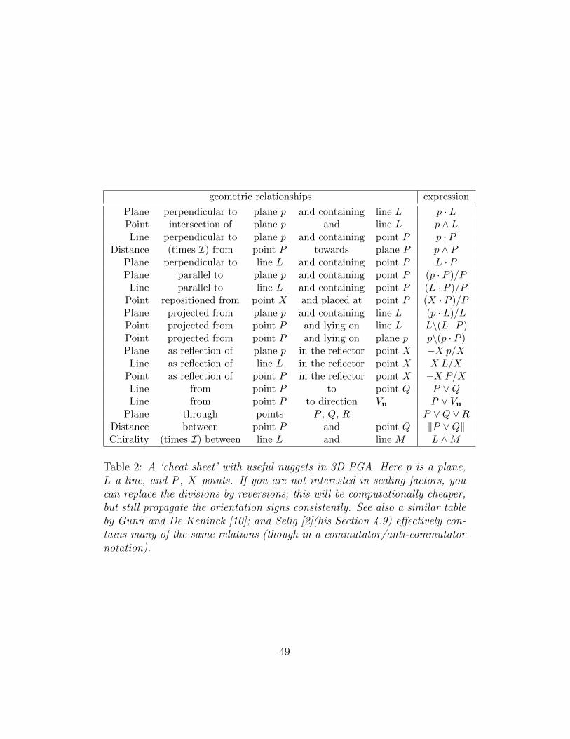
geometric relationships expression
Plane perpendicular to plane p and containing line L p · LPoint intersection of plane p and line L p ∧ LLine perpendicular to plane p and containing point P p · P
Distance (times I) from point P towards plane P p ∧ PPlane perpendicular to line L and containing point P L · PPlane parallel to plane p and containing point P (p · P )/PLine parallel to line L and containing point P (L · P )/P
Point repositioned from point X and placed at point P (X · P )/PPlane projected from plane p and containing line L (p · L)/LPoint projected from point P and lying on line L L\(L · P )Point projected from point P and lying on plane p p\(p · P )Plane as reflection of plane p in the reflector point X −X p/XLine as reflection of line L in the reflector point X X L/X
Point as reflection of point P in the reflector point X −X P/XLine from point P to point Q P ∨QLine from point P to direction Vu P ∨ Vu
Plane through points P , Q, R P ∨Q ∨RDistance between point P and point Q ‖P ∨Q‖Chirality (times I) between line L and line M L ∧M
Table 2: A ‘cheat sheet’ with useful nuggets in 3D PGA. Here p is a plane,L a line, and P , X points. If you are not interested in scaling factors, youcan replace the divisions by reversions; this will be computationally cheaper,but still propagate the orientation signs consistently. See also a similar tableby Gunn and De Keninck [10]; and Selig [2](his Section 4.9) effectively con-tains many of the same relations (though in a commutator/anti-commutatornotation).
49
6 Euclidean Motions
through Planar Reflections
We have designed PGA as an algebra of planes since we want to describeEuclidean motions by means of planar reflections. This follows the generalCartan-Dieudonne Theorem:
All orthogonal transformations in an n-D symmetric bilinear spacecan be constructed from at most n reflections.
It is immediately obvious that in 3D we can use two planar reflections toconstruct the two typical motions: rotations and translations. Using moreplanes combines such basic motions. But with 3D planes residing in a 4Drepresentational space, Cartan-Dieudonne states that there will not be mo-tions requiring more than 4 reflections. These multiple reflections have beengiven names:
• 0 reflections: the identity
• 1 reflection: a planar reflection
• 2 reflections: when the planes are parallel, this is a translation; whenintersecting, a rotation around the common line; when perpendicular,a line reflection
• 3 reflections: this adds an extra reflection to the previous case, andgenerates a glide reflection when two of the three are parallel, and arotoreflection then none are; when the three planes are perpendicular,this produces a point reflection
• 4 reflections: the general Euclidean rigid body motion, a ‘screw mo-tion’. We can factorize a general motion always as a rotation aroundan axis and a translation along that same axis (Chasles’ theorem). Wewill see that this description by means of four real reflections in realplanes corresponds, in its coordinate form, directly to the often-used19th century description of 3D rigid body motions by dual quaternions(which are often needlessly viewed as ‘complex’ in all senses of theword).
Let us find the versors corresponding to these multiple reflections in planes.
50
6.1 Multiple Reflection as Sandwiching
For the algebra of Euclidean directions, reflection of a direction vector x ina plane through the origin with normal vector n is the reflected direction−n x n−1 (if this is new to you, consult the earlier chapters of [1] or someother general text). This sandwiching operation:
x 7→ − n x n−1 (75)
then extends in two ways.
• It can be applied to any other element X of GA that we construct aslinear combinations of geometric products (and we have no desire tomake anything else)
X 7→ n X n−1, (76)
where X = (−1)grade(X)X, the grade involution, introduces a minus signfor the odd grade elements, and no sign for the even grade elements.
• We can perform sandwiching by repeated reflection in other elements.Associativity allows us to group those in versors, which are geometricproducts of invertible vectors. In a Euclidean geometric algebra, thislooks like (see Chapter 7 of [1]) a sandwiching product
x 7→ (−1)k (nk nk−1 · · ·n1) x (n−11 · · ·n−1k−1 n−1k )
= (−1)k (nk nk−1 · · ·n1) x (nk nk−1 · · ·n1)−1
= V xV −1, (77)
with the versor V defined as the product of k reflectors (and V ≡(−1)kV ). For motions, we are mostly interested in applying even ver-sors; then there are no signs to worry about.
• The inversion might seem somewhat expensive to perform – it is definedas V −1 = V /(V V ). But in PGA Rd,0,1, the denominator V V is alwayspositive since all Euclidean vectors have positive squares. So if youare only interested in results modulo a positive scaling factor (and incomputer graphics, that is often the case), then in the sandwich product
you can replace the inverse by the much cheaper reverse V (which ismerely a grade-dependent sign: a minus sign for the parts of grade 2and 3).
51
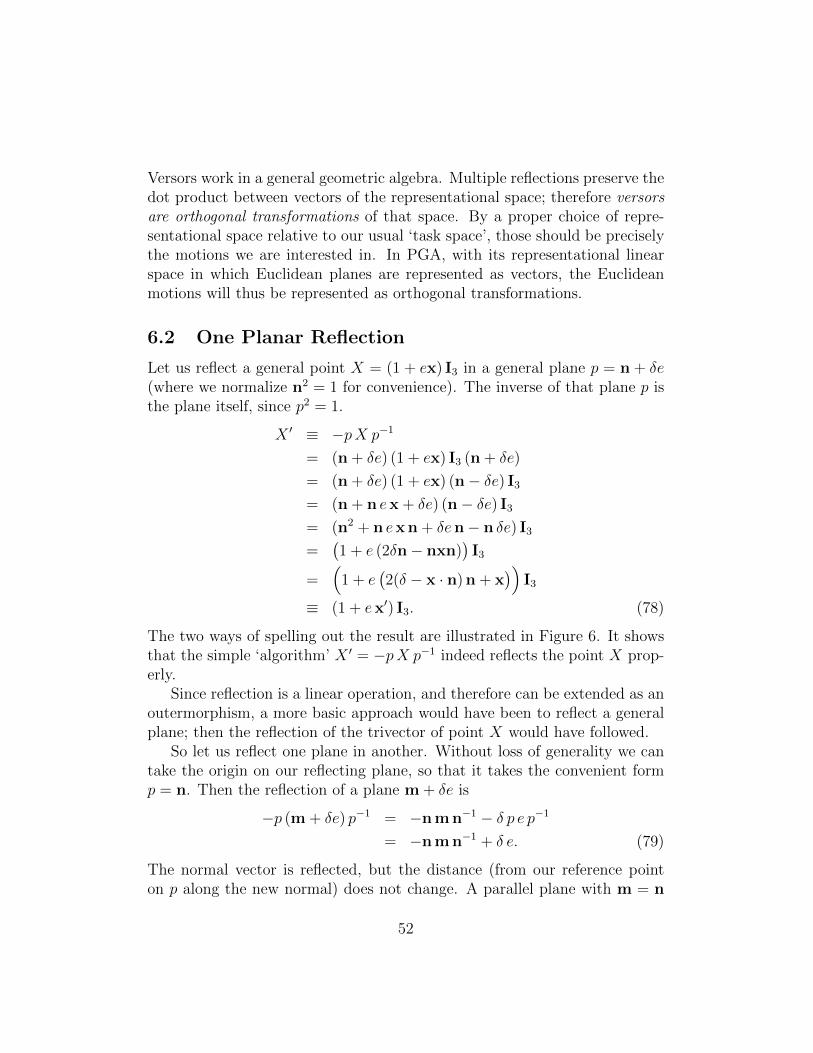
Versors work in a general geometric algebra. Multiple reflections preserve thedot product between vectors of the representational space; therefore versorsare orthogonal transformations of that space. By a proper choice of repre-sentational space relative to our usual ‘task space’, those should be preciselythe motions we are interested in. In PGA, with its representational linearspace in which Euclidean planes are represented as vectors, the Euclideanmotions will thus be represented as orthogonal transformations.
6.2 One Planar Reflection
Let us reflect a general point X = (1 + ex) I3 in a general plane p = n + δe(where we normalize n2 = 1 for convenience). The inverse of that plane p isthe plane itself, since p2 = 1.
X ′ ≡ −pX p−1
= (n + δe) (1 + ex) I3 (n + δe)
= (n + δe) (1 + ex) (n− δe) I3
= (n + n ex + δe) (n− δe) I3
= (n2 + n ex n + δen− n δe) I3
=(1 + e (2δn− nxn)
)I3
=(
1 + e(2(δ − x · n) n + x
))I3
≡ (1 + ex′) I3. (78)
The two ways of spelling out the result are illustrated in Figure 6. It showsthat the simple ‘algorithm’ X ′ = −pX p−1 indeed reflects the point X prop-erly.
Since reflection is a linear operation, and therefore can be extended as anoutermorphism, a more basic approach would have been to reflect a generalplane; then the reflection of the trivector of point X would have followed.
So let us reflect one plane in another. Without loss of generality we cantake the origin on our reflecting plane, so that it takes the convenient formp = n. Then the reflection of a plane m + δe is
−p (m + δe) p−1 = −n m n−1 − δ p e p−1
= −n m n−1 + δ e. (79)
The normal vector is reflected, but the distance (from our reference pointon p along the new normal) does not change. A parallel plane with m = n
52

X
X ′ = −pX p−1
p
O
X
X ′
δnx
2(δ − x · n) n
−n x n−1
2δn x′
Figure 6: A reflection of a point X into a single plane p (see on edge, ingreen) is in PGA simply computed as X ′ = −pX p−1 (left). When workedout in detail, that simple equation implements some fairly intricate geometry.The resulting position x′ can be made by adding a reflection −n x n−1 to twicethe support vector δn, or by twice adding, to the point position x, a relativedistance vector (δ − x · n) n. The result is the same, but the algebraic ‘code’is much more compact in PGA.
becomes−m+δe, so with opposite normal and at the other side of the mirror.If we conveniently take our arbitrary origin along the line of intersection ofthe planes, then δ = 0 and we see that this common line remains invariantunder reflection.
We emphasize that we should not just omit the minus sign in the defini-tion. If we reflect a plane parallel to the mirroring plane, we would expect itsnormal to flip sign, so that ‘back’ and ‘front’ are interchanged after reflection.With the minus sign as indicated, this is precisely what happens:
p 7→ − p p p−1 = −p. (80)
And of course a plane p′ perpendicular to the mirror (so with p′ · p = 0)retains its normal, as it should: −p p′ p−1 = p p−1 p′ = p′.
Many other sources on PGA unfortunately tend to neglect this sign in thebasic projection (perhaps because of the projective origins of PGA’s use of the
53
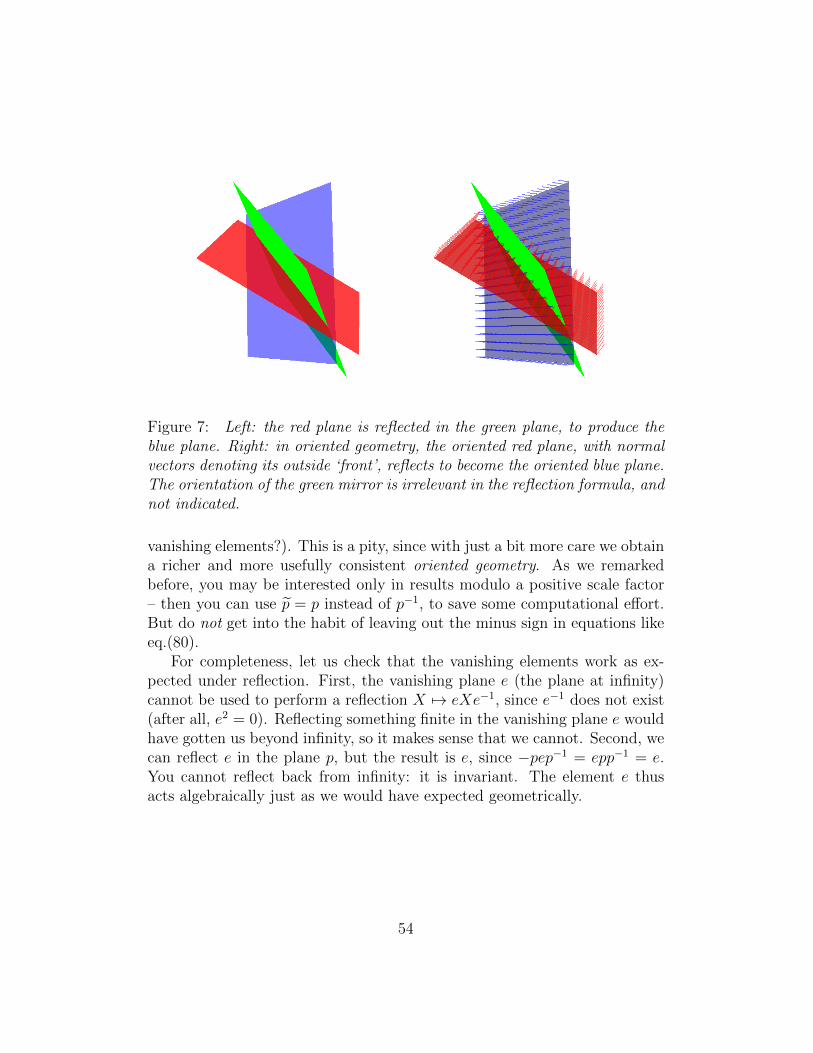
Figure 7: Left: the red plane is reflected in the green plane, to produce theblue plane. Right: in oriented geometry, the oriented red plane, with normalvectors denoting its outside ‘front’, reflects to become the oriented blue plane.The orientation of the green mirror is irrelevant in the reflection formula, andnot indicated.
vanishing elements?). This is a pity, since with just a bit more care we obtaina richer and more usefully consistent oriented geometry. As we remarkedbefore, you may be interested only in results modulo a positive scale factor– then you can use p = p instead of p−1, to save some computational effort.But do not get into the habit of leaving out the minus sign in equations likeeq.(80).
For completeness, let us check that the vanishing elements work as ex-pected under reflection. First, the vanishing plane e (the plane at infinity)cannot be used to perform a reflection X 7→ eXe−1, since e−1 does not exist(after all, e2 = 0). Reflecting something finite in the vanishing plane e wouldhave gotten us beyond infinity, so it makes sense that we cannot. Second, wecan reflect e in the plane p, but the result is e, since −pep−1 = epp−1 = e.You cannot reflect back from infinity: it is invariant. The element e thusacts algebraically just as we would have expected geometrically.
54

6.3 Reflections in Two Planes
The geometric product of two planes describes a double reflection. Let usstudy what form such a product can take. We can take normalized planeswithout loss of generality (since in the sandwich product we will use to applythe result to elements, the inverse that also occurs cancels any scale factor).
p2 p1 = (n2 + δ2e) (n1 + δ1e)
= (n2 · n1) + n2 ∧ n1 + (δ1n2 − δ2n1) ∧ e. (81)
There are some cases:
• Translation: If the planes are parallel, with n1 = n2 = n as commonunit vector, then the above evaluates to the translator
Tt ≡ 1 + (δ1 − δ2)n ∧ e ≡ 1 + et/2, (82)
with t defined as 2(δ2−δ1)n, double the separation vector of the planes.In the sandwiching with this element Tt, any element translates overt. Just to show how this produces the prefix operators we have seenbefore, let us translate the point at the origin in d-dimensional space,represented by Id:
(1 + ep/2) Id (1 + pe/2) = (1 + ep/2)(Id − p(−1)dIde/2
)= (1 + ep/2) (1 + ep/2) Id
= (1 + ep) Id, (83)
retrieving the point representation of eq.(13). On the other hand, trans-lating an origin plane n gives
(1 + ep/2) n (1 + pe/2) = n + ep n/2 + n e/2 + ep n p e/4
= n + (p · n) e (84)
which indeed retrieves the plane representation n+δe, with δ the signeddistance from the origin to the plane along the normal vector n.
A translator can alternatively be made as the ratio of two points, seeExercise 12.2:10, or of two parallel lines.
• Rotation at the Origin: Planes through the origin are not geo-metrically special (because the origin is not a geometrically significant
55
point). But let us see what kind of a motion two planes without dis-tance δi produce:
RφI ≡ p2 p1 = n2 · n1 + n2 ∧ n1 = cos(φ/2)− sin(φ/2) I. (85)
This is a purely Euclidean rotor for the rotation over φ, double theangle φ/2 between the planes. Note that I2 = −1.
We can decompose I on the coordinate 2-blade basis {e23, e31, e12},each of which squares to −1, and which have combination propertieslike e23e31 = e21 = −e12. In fact, setting i = e23, j = e31, k = e12, thealgebraic properties are isomorphic to those of a quaternion. So thereal 3D rotation operation RφI is algebraically like a quaternion. Butits derivation as the product of two planes feels quite different – anda lot more real and natural. We did not need to introduce complexnumbers to define it, just ratios of real planes through the origin.
• Rotation around a Line: Rotation around an arbitrary normalizedline L is also possible. To see the simple form it takes, let us constructit by a translation back to the origin, then a rotation at the origin,and placing it back again, so making TtRφIT
−1t . But the bivector I
around which this rotates should of course be parallel to the originalline L. Or conversely, L is the t-translated version of I, so L = Tt IT−1t .Performing the translation, the resulting operation is effectively thetranslated version of the rotor RφI, and can be expressed directly interms of the line L as
RφL ≡ cos(φ/2)− sin(φ/2)L. (86)
So in 3D PGA we can simply use a line L to produce a rotation aroundit.14 Note that L2 = −1, just as I2 = −1.
This is in fact algebraically isomorphic to how a dual quaternion (orbiquaternion) represents a 3D rotation. It uses elements from the full2-blade basis {e23, e31, e12, e01, e02, e03} (where we rewrote e as e0 forsymmetry and compactness). The three elements involving e = e0
square to 0, the others square to −1, and their mutual product prop-erties are precisely right for the dual quaternion functionality (as youmay verify in the Cayley table of Figure 1).
14In the next section, we will dare to rewrite this in exponential form as RφL ≡exp(−φL/2).
56
Dual quaternions therefore do not need to be introduced as doubly mys-terious entities, over an abstract algebra that contains both three complexnumbers and three dual numbers, somehow magically applicable to 3D mo-tions. The RφL above is simply a rotation operation around a real line L,obtainable as the product (or ratio) of two real planes having that line astheir intersection. When such a product of planes is applied in a sandwichproduct, it produces a rotation on any element. When the planes are par-allel, the rotation is around a vanishing line – we would usually call that atranslation. Get real!
6.4 Three Reflections; Point Reflection
This case contains just one extra reflection beyond the previous case, and isof less interest on a first pass through PGA.
We could study some things like glide motions, and factorize them inge-niously. In 2D such things have been done in the context of planar symmetrygroups. In 3D, this would produce the crystallographic groups. It is an in-teresting exercise to rewrite the CGA treatment of crystallographic groupsfrom [14] into PGA!
There is a special case, though, that deserves attention: if the threereflecting planes are perpendicular, their geometric product is identical totheir outer product. Therefore this is a reflection in a point. Devices withsuch three orthogonal planes are called retroreflectors - Apollo 11 put one onthe Moon, to determine its distance by bouncing laser rays off it, from theEarth.
We can most easily study the point reflection at the origin, for the pointO = I3. Then a general blade of the form X = TX + ePX reflects as
X 7→ −I3X I3
= −I3 (TX + ePX) I3
= −TX + ePX
= (−1) (TX − ePX). (87)
By factoring out the scaling by −1, we see that the positional aspect haschanged sign: so the result is a similar blade, but at the opposite side of O,and in opposite direction. We also see that the point reflection is a way ofproducing points of negative weight: for instance, O reflected in O gives −O.
57
In 2D PGA, a point reflection would be produced by its 2-blade points,such as the point at the origin I1 = e1 e2. Since this is even, the reflectionformula becomes X 7→ I2X I2 (no minus!), which for a blade X = TX+ePXproduces TX +e PX . Since for a blade the grades of tangential and positionalaspect differ by 1, this again results in a reversal of position relative to thereflection point. An overall sign reversal only happens for vectors of he 2DPGA, i.e., the 2D lines. This all makes sense, since in 2D a point reflectionis just a rotation over π.
6.5 Four Reflections: General Euclidean Motions(Oh and Incidentally Dual Quaternions)
According to Cartan-Dieudonne, in the 4D representational space of 3DPGA, four reflections will generate the most general orthogonal transfor-mation. So using the GA representation, the product of four general planevectors should produce a versor for the most general rigid body motion. Wecan rearrange these terms in different ways. In the usual classical represen-tation when using homogeneous coordinates, one typically views the generalmotion as a rotation at the origin followed by a translation. In PGA, thiswould be (reading right to left) a factorization in terms of two planes inter-secting in a line through the origin, followed by two planes intersecting in avanishing line.
((t + e/2) t
) (n2 n1
)∝ (1 + et/2) (cos(φ/2)− sin(φ/2) I) (88)
with φI the bivector angle from n1 to n2. The final form of representationis unique, though the four vector factors can be chosen with quite someleeway (as long as they produce the same φI and t). The element we haveconstructed is a rigid body motion versor, often called a motor.
But we have just seen how we perform rotations around a general line L, sorotations at the origin are no longer as special as they are in the classical vieworiginating in linear algebra. Therefore we could also characterize the generalmotion as a rotation around a general line L followed by a translation in thedirection of that line (this is in fact Chasles’ theorem on decomposition of 3DEuclidean motions). The former is the operation RφL, the latter translationeffectively ‘rotates’ around the vanishing line LI, so we could denote it asRδLI (we will see the exact reason behind this notation in Section 7). Then
58

the general motor is represented as the product
RδLI RφL = RφLRδLI . (89)
We can use either order, since the two operations commute. This is a naturalparametrization of a general motor: by one normalized oriented line L, anoriented angle φ and an oriented distance δ. It will take an even more conve-nient form in the exponential representation, in Section 7. This combinationgenerates a general element on the basis {1, e23, e31, e12, e01, e02, e03, e0123},with three basis bivector elements squaring to −1, and three squaring to 0.They are, again, dual quaternions, but now much less mysterious as ‘realscrews’.
6.6 The PGA Square Root of a Motor
Motors can be defined as the ratio of a (normalized) target blade B anda (normalized) start element blade A (obviously of the same grade), so asB/A – or as products of such ratios. (This uses the division by a blade,
which equals multiplication by its inverse A−1 = A/(AA); for a unit bladetherefore simply equal to its reverse.) However, B/A is not the motor thatcan be used in sandwiching to turn A into B, since it moves over twice therequired transformation. This deficiency is easily seen (taking normalizedblades for convenience): (BA−1)A(AB−1) = BAB−1 6= B.
To move A to become B, we actually need V =√B/A, as a sketchy but
plausible computation shows:√BA−1A
√BA−1 −1 =
√BA−1A
√A−1B = B.
(We can later improve on this derivation when we have the exponential andlogarithm of a motor, but this will do for now.) Therefore we need thecapability to take the square root of a motor.
In PGA, the square root of a normalized motor M (i.e., a motor that
satisfies M M = 1) is
square root of motor M :√M =
1 +M√2(1 + 〈M〉)
(1− 〈M〉4
2(1 + 〈M〉)
),
(90)where 〈M〉 denotes the scalar part of M , and 〈M〉4 the 4-vector part. Thiswas derived in [13] on CGA’s roots; but PGA’s are the same since it is asubalgebra of CGA. You may verify eq.(90) directly, by squaring and using
the normalization condition M M = 1 to rearrange terms.
59
The case of M = −1 is excluded, but this is not a problem geometrically:since the action of M and −M is the same we lose no significant meaning bydemanding, for instance, 〈M〉 ≥ 0 before applying the square root formula.
Apart from a scalar normalization eq.(90) is in essence
√M ∝ (1 +M) (1 + 〈M〉 − 1
2〈M〉4), (91)
which may be more efficient in applications where positive weighting factorsare not of interest. You would then use the reverse of this motor
√M at the
right hand side of the sandwiching – it is obtained by replacing M by M inthe first factor.
We use the term simple motor for a motor that has no grade 4 part. Itis typically made as the ratio of two vectors. In the exponential form wewill treat later, they are characterized as the exponential of a 2-blade (asopposed to a 2-vector). Because of the lack of a grade-4 part, we have forsimple motors
square root of simple motor:√M =
1 +M√2(1 + 〈M〉)
∝ 1 +M. (92)
In 2D PGA, all motors are simple (there is literally no space for them not tobe!), so this square root formula applies there universally. In spaces of morethan 5 dimensions, terms of grade 6 would appear and one would need togeneralize the square root of eq.(90). But for now, we will not go there.
Having square roots of motors is not only required for determining thecorrect motor from a blade ratio; it is also convenient to have when interpo-lating motions. Each motion can be halved by its square root, and repeatedhalving gives a simple form of interpolation by subdivision. A more generalinterpolation, employing n-th roots, can be performed after we have deter-mined motor logarithms in Section 7.3.
6.7 Example: Universal Motors
As a simple demonstration of the universality of PGA when acting on geo-metric elements, consider Figure 8. It contains a green triangle T with threevertices, the trivector points T1, T2 and T3. There is a yellow plane p, con-structed from a point Q and a normal vector n as p = (n · Q)/Q. A redline L (normalized) is running in direction u, so it can be constructed froma point on it and the vanishing point euI3 (as in eq.(38)).
60
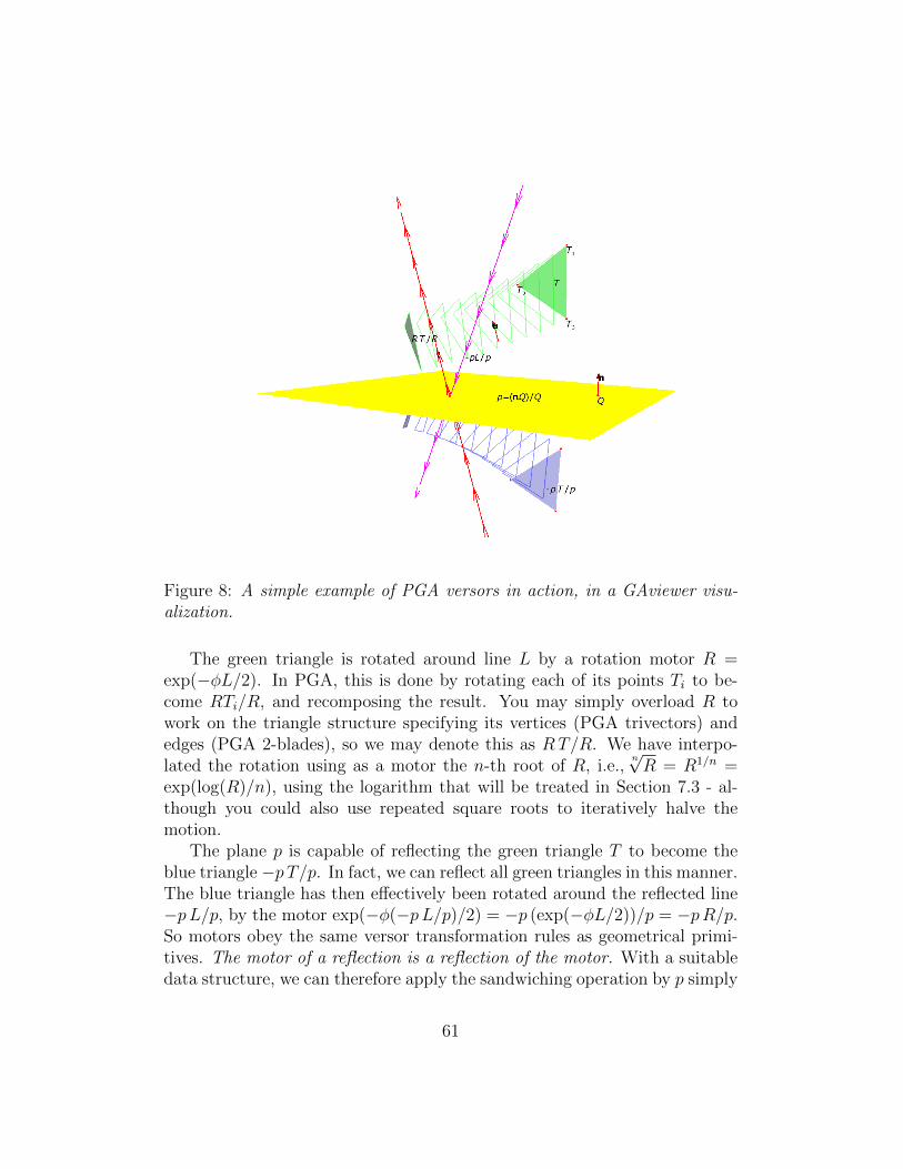
Figure 8: A simple example of PGA versors in action, in a GAviewer visu-alization.
The green triangle is rotated around line L by a rotation motor R =exp(−φL/2). In PGA, this is done by rotating each of its points Ti to be-come RTi/R, and recomposing the result. You may simply overload R towork on the triangle structure specifying its vertices (PGA trivectors) andedges (PGA 2-blades), so we may denote this as RT/R. We have interpo-lated the rotation using as a motor the n-th root of R, i.e.,
n√R = R1/n =
exp(log(R)/n), using the logarithm that will be treated in Section 7.3 - al-though you could also use repeated square roots to iteratively halve themotion.
The plane p is capable of reflecting the green triangle T to become theblue triangle −p T/p. In fact, we can reflect all green triangles in this manner.The blue triangle has then effectively been rotated around the reflected line−pL/p, by the motor exp(−φ(−pL/p)/2) = −p (exp(−φL/2))/p = −pR/p.So motors obey the same versor transformation rules as geometrical primi-tives. The motor of a reflection is a reflection of the motor. With a suitabledata structure, we can therefore apply the sandwiching operation by p simply
61
to all elements ‘above’ the plane, to get the elements ‘below’ - even includingthe counterrotation that acts there.
You can view this setup flexibly in 3D and play with it (by changing thedefining geometrical parameters) in ganja at https://enkimute.github.
io/ganja.js/examples/coffeeshop.html#chapter11_motors. Since thecode is javascript, you can modify the scene, confirming how easy it is totransform in PGA.
6.8 Example: Reconstructing a Motorfrom Exact Point Correspondences
Let us assume that we have three normalized labeled points A, B, C (noton a line), and that we know where an exact motor sends each of them, toA′, B′, C ′, with the same weights. We would like to reconstruct that motor.Here is how we could proceed:
1. First align A to A′. This is done by the motor
VA =√A′/A, (93)
which thus achieves A′ = VAA VA (it is of course a translation, see Ex-ercise 12.2:10). When we apply this motor to B′ and C ′, they have be-come slightly better aligned, and now only the new relative positions toA′ matter. The new subproblem thus involves aligning BA ≡ VAB VAwith B′ and CA ≡ VAC VA with C ′.
2. Now align BA with B′ while preserving the result on A. That requiresan additional motor that aligns the line A′ ∨BA with the line A′ ∨B′,through
VB =√
(A′ ∨B′)/(A′ ∨BA). (94)
This motor VB leaves A′ invariant, and rotates BA into B′.
The total motor so far is then VB VA, which aligns both A and Bto A′ and B′, and transforms C to CBA ≡ VB VAC VA VB (or CA to
CBA ≡ VB CA VB).
3. Finally, align CBA to C ′ by aligning the plane A′ ∨ B′ ∨ CBA withA′ ∨B′ ∨ C ′, keeping the line A′ ∨B′ and the point A′ invariant. Thisrequires the motor
VC =√
(A′ ∨B′ ∨ C ′)/(A′ ∨B′ ∨ CBA). (95)
62
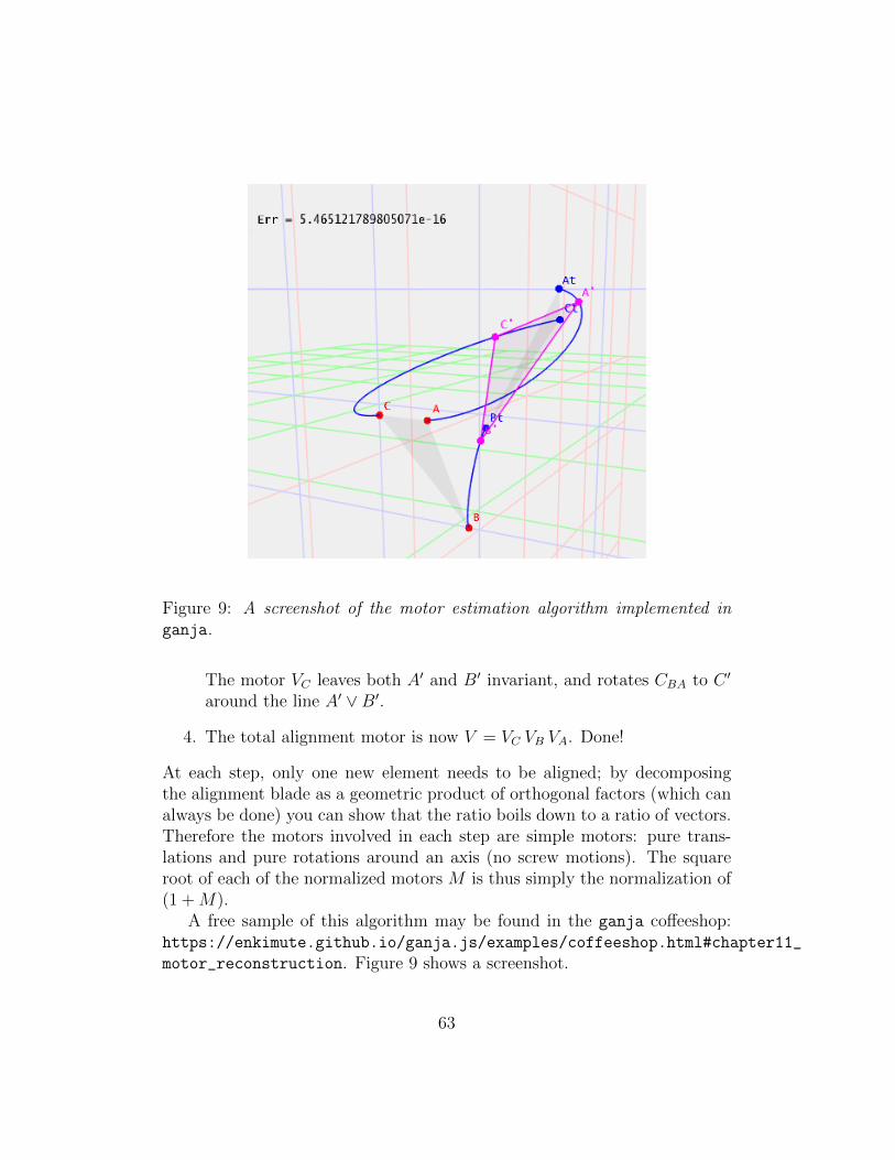
Figure 9: A screenshot of the motor estimation algorithm implemented inganja.
The motor VC leaves both A′ and B′ invariant, and rotates CBA to C ′
around the line A′ ∨B′.
4. The total alignment motor is now V = VC VB VA. Done!
At each step, only one new element needs to be aligned; by decomposingthe alignment blade as a geometric product of orthogonal factors (which canalways be done) you can show that the ratio boils down to a ratio of vectors.Therefore the motors involved in each step are simple motors: pure trans-lations and pure rotations around an axis (no screw motions). The squareroot of each of the normalized motors M is thus simply the normalization of(1 +M).
A free sample of this algorithm may be found in the ganja coffeeshop:https://enkimute.github.io/ganja.js/examples/coffeeshop.html#chapter11_
motor_reconstruction. Figure 9 shows a screenshot.
63

Very similar algorithms to the above can be designed to find the motorthat transforms three corresponding plane pairs (easy), or three line pairs(harder!).15 See our structural exercise 12.2:11.
6.9 Summary
General Euclidean transformations can be generated by multiple reflectionsin planes. In PGA this produces versors, the usual geometric algebra oforthogonal transformations.
We explicitly derived the versors for some of the basic motions, and con-nected those real constructions briefly to the complex encoding by quater-nions or dual quaternions which is more commonly taught. Incidentally wesaw that in PGA a pure rotation is a rotation around any line, rather thanaround a line through the origin (as it is in linear algebra).
We showed how versors are applied universality to all elements, primitivesand operators alike, by a simple sandwiching construction eq.(77). Thisenormously simplifies and reduces implementation code.
Versors are easy to make from elements by geometric product ratios.But the ratio of elements does not quite give the versor transforming one tothe other, you need to take a square root. So we exposed the square rootformula for PGA in eq.(90), including the simplified form eq.(91) it takeswhen magnitudes are less important in your application.
15In [15], a structurally identical algorithm was used to perform alignment of directionsin 3D (so using only the rotors in the 3D GA of Chapter 10 in [1]). It resulted in anefficient formula that was directly usable in the more traditional quaternion formulation,and that appeared to be new. The geometrical approach, viewing a quaternion as theratio of two planes, paid off! It may be possible to derive a similar closed form expressionfor our final result, giving a compact formula for the dual quaternion that aligns the tripleof points (though it appears at first try that it has too many terms to be memorable).
64

7 The Exponential Representation
We have constructed the rigid body motions as products of planes, or ratiosof flats. But in practice it is often more convenient to synthesize them asexponentials, since that parametrizes them straightaway by geometricallyrelevant elements: direction of motion for a translation, axis and angle for arotation, and screw and pitch for a general rigid body motion. This approachworks for the ‘proper’ motions, not for the reflections. So in this section ourversor contains an even number of terms, and is thus an even multi-vector,a member of the even subalgebra R+
3,0,1 of 3D PGA.
7.1 Exponentiation of Invariants Gives Motions
We have seen how a rotation versor can be formed as the product of tworeflection planes V = p2 p1, and that it rotates around their common line.That line is represented as L = p1∧p2, and it would be nice if we could writethe versor in terms of it: for many pairs of planes could have that uniqueline L in common, and we prefer our parametrizations as unambiguous aspossible. In geometric algebra in general, we can perform exponentiation (asexplained in Chapter 7 of [1]) of bivectors to produce even versors. (This isintimately related to the classical description of motions through their Liealgebra, but we will just absorb this rather than spell it out, referring toe.g., [16] for details.)
We will employ the standard notation of even versor application, in whicha normalized bivector B produces a versor Vτ = exp(−τ B/2). (This versor
is even a rotor, since V V = 1, and therefore V −1 = V .) This versor Vτ isapplied to an arbitrary element X by a sandwich product, to produce anorbit parametrized by τ as
Xτ = Vτ X V −1τ = e−τB/2X eτB/2. (96)
As we have seen when constructing versors by multiple reflections, such atransformation is linear in X, and it preserves grades. Moreover, versorstransform the geometric product covariantly:
V (a b)V −1 = (V a V −1) (V b V −1), (97)
and since outer and inner products are linear combinations of geometric prod-ucts, it does the same for them. Products involving duality (like the join)
65
also transform covariantly under even versors, since they have determinant+1, and therefore do not affect the sign of the pseudoscalar. The sandwich-ing product is thus an obviously structure-preserving way of transformingelements.
Let us show such exponentiation for rotations around the line L = p1∧p2.We normalize L such that ‖L‖ = 1. Such a line squares to L2 = −1. Thisis most easily seen if we construct it as the intersection of two orthogonalnormalized planes (so p21 = p22 = 1 and p1 · p2 = 0). Then p1∧ p2 = p1 p2, and
L2 = (p1∧p2) (p1∧p2) = p1 p2 p1 p2 = −p1 p1 p2 p2 = −(p1)2 (p2)
2 = −1. (98)
Therefore using L in an exponentiation produces trigonometric functions, inthe usual way:
exp(−φL/2) = 1− 11!φL/2 + 1
2!(φL/2)2 − 1
3!(φL/2)3 + · · ·
= cos(φ/2)− sin(φ/2)L. (99)
Note that the line L remains invariant under this operation, and that themotor is the exponential of the invariant. That turns out to be very usefulgeneral principle to construct specific motors!
Translation versors (of the form of eq.(82)) involve direction elements likeet, which can be seen as a vanishing line, the locations where the plane t(with normal vector t) meets the vanishing plane e. Such elements square tozero, since e2 = 0:
(et)2 = e t e t = −t2 e2 = 0. (100)
Therefore we can also make translation versors by exponentiation
exp(et/2) = 1 + 11et/2 + 1
2(et/2)2 + · · ·
= 1 + et/2, (101)
completely conforming to the form they took when constructed from reflec-tion in two parallel planes in eq.(82).
When translating orthogonally to a plane p = n + δe with normal vectorn, the vanishing line en = ep remains invariant. And the correspondingtranslation operator is indeed the exponential of this invariant: exp(ep).
Composing a general rigid body motion from an origin rotation (withL = I = e1 e2 on an orthonormal basis) followed by a translation yields a
66

versor that is commonly called a motor:
M = exp(et/2) exp(−φI/2)
= (1 + et/2) (cos(φ/2)− sin(φ/2) I)
= cos(φ/2)− sin(φ/2) I + et/2 cos(φ/2)− sin(φ/2) e t I/2. (102)
A general motor M therefore contains grades 0, 2 and 4. Note that younever have to write out such expressions explicitly, we just worked this outin components to give you a feeling for the internal structure. But we havealready mentioned that there is a better parametrization of motors, accordingto Chasles’ decomposition, in eq.(89): a rotation around a line, combinedwith a translation along that same line. In exponential form, that becomes
M = RδLI RφL = exp(δLI/2) exp(−φL/2) = exp(−φL/2 + δLI/2), (103)
where the combination into a single exponent is permitted since the L andLI commute. Both the Euclidean line L and the vanishing line LI areinvariant under this rotor M , so this is again of the form ‘exponential of theinvariant’. The ratio δ/φ is the pitch of the resulting screw motion, indicatingthe amount of translation per turn.
7.2 Child’s Play
Let us enjoy an intuitive example showing how the continuity of our expe-rience in rotation and translation is faithfully represented in PGA, and hownatural it is to exponentiate geometrically invariant elements to produce mo-tors.
Mia-Lou wants to ride her tricycle. She starts at the origin, facing inthe e1 direction. Let us denote the plane perpendicular to the ground planee3 and containing her rear axle by r, and the plane perpendicular to theground plane containing her front axle by f . The latter plane depends onher steering angle φ, so let us denote it as f(φ). With the trike assumed tobe of unit length, we have in coordinates:
r = e1 and f(φ) = (e1 cosφ+ e2 sinφ) + e cosφ. (104)
The two planes meet in r∧f(φ), and this is the center of her motion: it staysinvariant as she moves with constant steering angle φ. Therefore Mia-Lou’smotor is a power of:
exp(r ∧ f(φ)) = exp(e1e2 sinφ+ e1e cosφ). (105)
67

φ
center
orbit
r = e1f(φ)
O
Figure 10: Geometry and orbits of a tricycle. When moved one time-unitunder the motor Mφ = exp(r ∧ f(φ)/2), the endpoints MφOMφ, for varioussteering angles φ, appear to form a cardioid.
We will not normalize the bivector argument and then introduce an anglemeasure, but rather take the magnitude of the meet as the amount of motion(which can be further parametrized by a time t, as in exp(r∧f(φ)t), to travelfractional amounts).
It is clear from this formulation that there are no discontinuities in themotor. When φ = 0, the motor is exp(e1e), a purely translational motionover 2 units of length. The invariant center is now a vanishing point (atinfinite distance to her left or to her right). As φ increases, the motionbecomes rotational around a finite turning center at her left, with an everdecreasing turning radius. Then, when Mia-Lou has her handlebars at anangle of π/2, the motion is purely rotational around the pivot point on therear axle, by motor exp(e1e2) over an angle of 2 radians. If we motorize herfront wheel (so that she can even move when the angle exceeds π/2), shemoves backwards around a turning point at her right. A 180-degree turnof the handlebars has her driving straight back to her father, by the motorexp(−e1e).
And the same sequence applies to her steering to the right, by negativeangles φ. Starting from steering straight ahead, the center of rotation thusmoves smoothly from infinity to either her left or right, and even to the pointon the rear axle for a pure rotation when φ = π/2. At no point is there aneed for a conditional statement to switch motion state – the one motor
68

exp(r ∧ f(φ)) covers all motions without discontinuity.Figure 10 shows a screenshot of a demo of Mia-Lou’s trip. It is a nice
geometrical fact that a unit motion in the motor exp(r ∧ f(φ)) moves theoriginal midpoint of the rear axle to an endpoint that lies on a cardioid. Youmight try to prove that!
You can play with this demo in ganja at the link https://enkimute.
github.io/ganja.js/examples/coffeeshop.html#chapter11_tricycle&fullscreen.Wait half a minute for it to load; the slider to adjust the steering angle is atthe top.
7.3 The PGA Motor Logarithm
As eq.(103) shows, a general motor is the exponential of a bivector. If wewant to interpolate the motion, we need that bivector; to retrieve it, giventhe motor, we require a logarithm. For the non-commuting elements of PGA,this requires some care. First, since a versor V and its negative −V have thesame effect, let us assume that our versors have a non-negative scalar part;it makes the essence of the logarithms simpler to express.16
A simple motor is the exponential of a 2-blade. The logarithm of a simplemotor of the form exp(2-blade) is easy to extract by the considering its scalarand 2-blade components: it is proportional to the 2-blade by a factor thatcan be deduced from the magnitudes of the terms. In PGA, there are twocases:
• R = exp(B) with B2 < 0 (rotation).Then define ‖B‖ =
√−B2, and write B = ‖B‖B, so that B2 = −1.
Expand the motor to R = cos(‖B‖) + sin(‖B‖)B and it is then clearthat the principal logarithm is, in terms of the k-grade selection oper-ator 〈 〉k,
log(R) = atan(‖〈R〉2‖〈R〉0
) 〈R〉2‖〈R〉2‖
≡ atan(〈R〉2〈R〉0
), (106)
where the second rewriting effectively defines a GA atan function onbivector arguments, to return a bivector. In this case, log(R) is pro-portional to the invariant rotation axis.
16There are some more advanced reasons to discriminate between V and −V , in certainapplications of multiple connected objects, but we will not use that in this text. ConsultChapter 7 of [1] if you are interested.
69
• T = exp(B) with B2 = 0 (translation).We can expand this motor to T = 1 +B, so the logarithm is simply
log(T ) = 〈T 〉2 = T − 1. (107)
This logarithm is proportional to the invariant vanishing line.
But for a general motor, of the form exp(bivector), the basic puzzle is thatthe individual components of a general bivector do not commute; thereforewe cannot write the exponential of their sum as a sum of exponentials (whichwould give a product of simple motors and make their logarithms easy). Thesolution is to write a general bivector as the sum of two commuting 2-blades;then we can perform the split, and are left with a product of commutingsimple motors. We have already performed this split in Section 5.6, but weare only half done: we should retrieve the 2-blade parts not from B, but fromV = exp(B).
Studying the expansion of the motor in factorized form in terms of theunit lines L and LI shows how we can proceed:
V = exp(B)
= exp(αL+ βLI)
= exp(αL) exp(βLI)
= (cosα + sinαL) (1 + βLI)
= cosα + sinαL+ β cosαLI − β sinα I= cosα
(1 + tanαL+ β LI − β tanα I
). (108)
In this expansion, almost all information for the logarithm is contained in thebivector part of the versor, especially since we can retrieve the coefficients ofits decomposition into commuting 2-blades by eq.(69). We then merely applysome function to the weights to retrieve the actual parameters of rotation
70

and translation. This leads to the motor logarithm
W = 〈V 〉2/〈V 〉0, (109)
α = atan(√
W · W), (110)
βI =W ∧ W
2√W · W
, (111)
L =W√W · W
(1− 1
2
W ∧ WW · W
), (112)
log(V ) =(α + βI
)L. (113)
Again, this does not work when W 2 = 〈V 〉22 = 0, but we have seen that thelogarithm in that purely translational case is extremely simple, see eq.(107).It also fails when 〈V 〉0 = 0, but then α = π/2 and the rest of the formulascan use W = V . The result of the logarithm is now the sum of the invariantrotation axis and the invariant vanishing line (or ‘translation axis’).
In 2D PGA, motors are simpler, because they are always already theexponent of a 2-blade (since in the 3-dimensional representation space, all2-vectors are 2-blades). In 2D PGA the logarithm thus simplifies to
W = 〈V 〉2/〈V 〉0 and log(V ) = atan(√
W · W) W√
W · W, (114)
except when W · W = 0 (the translation case); then log(V ) = V − 1.When extracting logarithms, please realize that a versor is always of the
form V = exp(−B/2), so that retrieval of the actual generating B (if that iswhat you are looking for) requires B = −2 log(V ).
7.4 Summary
The exponential form of an even versor allows direct and unique parametriza-tion of an elementary (screw) motion by its invariant bivectors (basically, thelines that are not affected).
Conversely, retrieving the invariants requires a logarithm. We derivedthat in some detail, to a fairly compact final result eq.(109)-eq.(113) Theelementary motion can then be interpolated.
71

8 Oriented Euclidean Geometry
The expressions we compute are not only purely geometrically interpretablein terms of positions and attitudes, but they also have magnitudes and signs.In a purely projective approach to PGA, we would neglect those; but theyturn out to give useful quantitative information, and also permit us to de-fine ‘inside/outside’ and chirality (‘handedness’) consistently. We have sofar drawn little attention to this possibility, since we wanted to show thegeometry first.
In image synthesis applications, the neglect of positive weighting fac-tors usually makes good sense: it does not change where you draw things.However, the signs of products consistently propagate ‘direction of travel’,‘reflection from the outside’, ‘consistent normal directions’, et cetera, andtherefore should be kept for interpretation and generation.
In 3D scene analysis, on the other hand, the numerical factors are highlyindicative of quantitative aspects of the scene, related to useful measuresand stability: ‘do these three points join to form a reliable plane’, ‘is thisintersection point sensitive to perturbation’, etc.
In all we have done so far, we carefully kept the signs and weightingfactors. We now should provide some ways to interpret them. You will findthat some of these meanings sound annoyingly hard to remember; we areapparently not too naturally sensitive to such aspects of geometry. But ifyou want to compute with them in a consistent manner, geometric algebragives you the tools.
Whichever field you are in, get into the good habit of not being sloppywith the signs, even if you do decide to ignore the magnitudes. Signs give youan oriented geometry in which you will not need to reconstruct orientationsafterwards, but can carry them along consistently in your computations.
8.1 Ordering
Some of the signs we will obtain are not so much due to the orientations ofthe objects we combine, but to the order in which we combine them. Let usget that out of the way first, notably for the meet and join operations.
• Ordering the meet.Since the meet is an outer product, the effect of changing the order of
72

two arguments A and B with grades a and b, respectively, is
A ∧B = (−1)abB ∧ A. (115)
Thus a line that is the meet of two planes p1 and p2 obtains the oppositeorientation if we compute it as the meet of p2 and p1. Our eq.(9) showsthat the direction vector of the line p1 ∧ p2 is the 3D cross productn1×n2 of the normal vectors of the planes, in that order (for our right-handed coordinate system). The magnitude is the sine of the anglebetween the normal vectors, which is indeed an odd function, so as theplanes ‘hinge across’ each other, the sign changes.
• Ordering the join.The sign incurred in swapping the arguments of the join (let us call itthe ‘swap sign’) depends on the dimension of the space it is computedin. For PGA, that space is (d+ 1)-dimensional, and we have
A ∨B = (−1)(d+1−a)(d+1−b)B ∨ A. (116)
Thus a line that is the join of two points P and Q (which are d-bladesof PGA) satisfies P ∨ Q = −Q ∨ P , in any dimension. A line canthus be given an orientation by joining points in a chosen order. Butbeware: those points themselves should be translated versions of thepoint at the origin Id, i.e., they should be positively proportional to theEuclidean pseudoscalar that was chosen for the space. Since negativepoints can result from operations (such as reflection or meet), this maybe an issue in your subsequent constructions.
Looking at these swapping signs, we thus find that in 3D PGA (so for d = 3),the swap signs of meet and join are the same. Note that any combinationinvolving a 3D line L (which is a 2-blade) will be symmetric:
A ∧ L = L ∧ A and A ∨ L = L ∨ A, for a line L. (117)
For quick reference, we show the swap signs for meet and join in Table 3.Where these signs are negative, we have to be careful in how we combine theelements, since the signs we obtain will be partly non-geometrical, merelycaused by the way we phrased the question of ‘how they met’, and ‘when theyjoined’. That does not make the answers useless, but definitely potentiallyconfusing. In 3D the rule is: only if both arguments are odd, there will be aminus sign in the swapping for both join and meet.
73

∧, ∨ 0 1 2 3 40 + + + + +1 + − + − +2 + + + + +3 + − + − +4 + + + + +
∨2D 0 1 2 30 − + − +1 + + + +2 − + − +3 + + + +
Table 3: Signs incurred when swapping the arguments of n-D meet and 3Djoin, and of the 2D join (denoted ∨2D). The signs for the 2D meet are asfor the 3D meet.
8.2 A Line and a Plane Meet
When (in 3D) a line L and a plane p meet in a point, the sign of theirmeet is independent of their order. So that sign has a geometric significanceindependent of convention. Moreover, though the geometric location of thecommon point depends on the precise location of line and plane, both thescalar factor (containing its ‘strength’ of meeting) and its sign (denoting the‘kind’ of incidence) do not depend on their location, but only on their relativeattitude. We can therefore most easily acquire an intuition of the sign andmagnitude of the meet by simply computing how it looks at the origin.
So we calculate the meet of a line with direction u through the origin(which is L = uI3), with a plane with normal n through the origin (which isp = n). Let us take both as being normalized, so u2 = 1 and n2 = 1. Thenwe compute
p ∧ L = n ∧ (uI3) = (n · u) I3. = (n · u)O, (118)
where O = I3 is the normalized point at the intersection point, in this casethe origin. We thus find that there is a ‘meeting strength’ equal to the cosinebetween line direction u and the plane normal n: the meet is strongest whenthe line is perpendicular to the plane, and zero when the line lies within theplane (which is a degenerate situation for this linearized form of intersec-tion). We also see that the intersection point is positively proportional toO = I3 when the line direction and plane normal are in similar directions(positive cosine), and negative when opposite. The distinction is requiredfor applications like ray tracing, where the plane would denote a locally flatpiece of boundary and one would want to know whether an incoming ray
74
could validly hit it from the outside, or invalidly from the inside.So this is how negative points get into our algebra: the signs indicate
how the points were made. Be aware of such possible signs in subsequentcomputations with those points; you may want to normalize them to positivebefore you use them, so that you can keep the orientations of compositeobjects clear in their meaning.
The sign is unavoidable, since changing the order of the arguments has noeffect. So if we would prefer to have a convention in which the intersectionpoint of ray coming in from the outside of a planar boundary is positive (i.e.,to be a translated positive multiple of O = I3), then we would have to enforcean encoding convention in which n is the ‘inside pointing normal’.
8.3 The Join of Two Points
As we saw above, the join of two points is a line whose orientation (the signof its direction vector) depends on their order, in any dimension, and this isprecisely as we would like it. The line determined by P and Q, which is P∨Q,should have the opposite sign of the line Q ∨ P determined by Q and P . Inthis case, the magnitude of the join of two normalized points is proportionalto their distance (as we compute below); including the orientation, we couldsay it is their signed distance.
We repeat the explicit expression for the line P ∨Q of eq.(37):
P ∨Q = (q− p) I3 + e(12(p + q) ∧ (q− p)
)I3. (119)
For simplicity (and without loss of generality due to the translation covari-ance of the join in PGA), let us take p = 0 so that P = O = I3:
O ∨Q = q I3. (120)
This is a line through the origin with direction vector q. To be precise, theresulting line has the same direction as q, with a magnitude equal to thedistance of O to Q. So the 2-blade O ∨ Q represents the line from O to Q,with a ‘strength’ (or ‘velocity’) ‖q‖.
The pleasant result that the reading order is the order of connecting-the-dots is due to our non-standard form of the Common Factor Axiom eq.(25).The desirability of this ordering was our reason for deviating from [8], byeffectively swapping the order of arguments relative to their join.
75
8.4 The Meet of Two Planes
The meet of two planes also results in a line, this time oriented in the waywe might expect in a space with right-handed pseudoscalar. Again the ordermatters: since both planes are odd, there is a swap sign. Let us check theresult at the origin, with two planes p1 = n1 and p2 = n2, both normalized.Then
p1 ∧ p2 = n1 ∧ n2 =((n1 ∧ n2) I−13
)I3 = (n1 × n2) I3, (121)
with × the 3D cross product. The final rewriting was our way of describingthe direction of a line by means of a Euclidean vector, as explained in eq.(9).
8.5 The Meet of Plane and Point: Inside/Outside
When a plane and a point meet, the result is a PGA 4-vector, as we saw inSection 2.7. Yes, even a point not on the plane has a meet with it; for themeet is not a geometric intersection of point sets.
For simplicity, let us first do the case where P = O, the point at theorigin. There is a swapping sign (both are odd) so the order matters.
p ∧O = (n + δe) ∧ I3 = δ e I3 = δ I. (122)
The plane representation n + δe is of a plane with normal vector n and asupport vector of δn, in the positive n-direction; thus the point at locationδn is on the plane.
We now find that we can retrieve δ as the strength (or rather, weakness)of the meet of plane with point O at the origin: it is the proportionalityfactor with the pseudoscalar I. We can interpret this factor therefore as thedistance the point O has to travel in the direction of n to become a point onthe plane.
For a plane p and general point X, we get p ∧ X = (δ − n · x) I, andthe interpretation is the same: the factor of the pseudoscalar denotes howmuch we should move X to get onto p. If it is positive, X lies on the side ofthe plane that n points away from. If we wish to call that positive side theoutside of the planar border, then n should be the ‘inward pointing normal’.
8.6 The Meet of Two Lines: Chirality
The meet of two lines has no swapping sign, and is therefore a geometricproperty independent of any convention on ordering (though it will depend
76
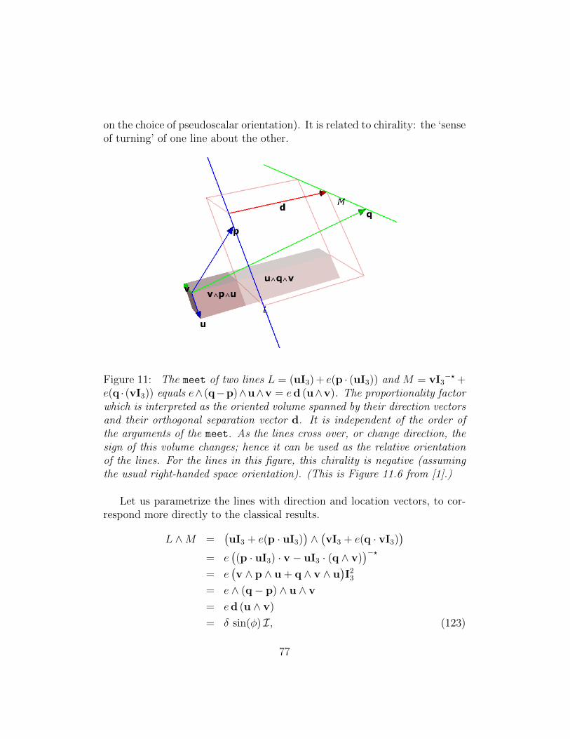
on the choice of pseudoscalar orientation). It is related to chirality: the ‘senseof turning’ of one line about the other.
Figure 11: The meet of two lines L = (uI3) + e(p · (uI3)) and M = vI3−? +
e(q · (vI3)) equals e∧ (q−p)∧u∧v = ed (u∧v). The proportionality factorwhich is interpreted as the oriented volume spanned by their direction vectorsand their orthogonal separation vector d. It is independent of the order ofthe arguments of the meet. As the lines cross over, or change direction, thesign of this volume changes; hence it can be used as the relative orientationof the lines. For the lines in this figure, this chirality is negative (assumingthe usual right-handed space orientation). (This is Figure 11.6 from [1].)
Let us parametrize the lines with direction and location vectors, to cor-respond more directly to the classical results.
L ∧M =(uI3 + e(p · uI3)
)∧(vI3 + e(q · vI3)
)= e
((p · uI3) · v − uI3 · (q ∧ v)
)−?= e
(v ∧ p ∧ u + q ∧ v ∧ u
)I23
= e ∧ (q− p) ∧ u ∧ v
= ed (u ∧ v)
= δ sin(φ) I, (123)
77
where we factorized orthogonally by the orthogonal separation vector d ≡((q− p) ∧ u ∧ v
)/(u ∧ v) (from L to M), see Figure 11.
The result of L ∧M is proportional to the pseudoscalar I, by a signedquantity of which the magnitude is the product of the line separation δ (fromL to M) and the sine of the angle between u and v (from the L-directionvector u to the M -direction vector v).
That factor (and with it the meet result itself) is therefore an interestingmeasure that combines spatial and angular distances: it is zero when thelines intersect, but also when the lines are parallel (which is of course alsoan intersection, in a common vanishing point).
The chirality is the sign of the proportionality factor, which is also thesign of the scalar (d ∧ u ∧ v)/I3. Thus if we follow line L in its direction uand then find ourselves moving around line M such that u, v and d forma frame of the same orientation as I3, we call the chirality positive; and ifnot, negative (or zero). Figure 11 shows an example of negative chirality ina space with right-handed pseudoscalar.
8.7 Summary
In this text we really tried to use the capability of PGA to propagate orienta-tion signs carefully, since they are so useful in practice. We showed that thisis possible, but it takes some getting used to. To interpret them properly,we need to distinguish between ‘geometrical signs’ and incidental signs fromconstruction order. But both are useful tools.
The emphasis on these aspects is rather new. We believe PGA is a goodalgebraic framework to encode the oriented projective geometry of Stolfi [17],and we would expect this field to develop more than we could indicate in thisintroductory text.
78

9 Projective Duality in PGA
The original meaning of the P in PGA is ‘projective’ [12], since it was derivedin the context of a projectivization of Euclidean space (i.e., adding points atinfinity as regular elements). As usual in a projective approach, there isa natural duality between points and hyperplanes, between k-blades and(n − k)-blades. To fully represent this duality relationship, one needs tomaintain both PGA and its dual space (or combine both in one), with bothe and er in their bases – as we temporarily did when motivating the join inSection 3. In this full space the duality between points and hyperplanes canbe represented naturally; both types of elements are represented distinctlyand explicitly.
When limiting ourselves to only the PGA space spanned by {e, e1, e2, e3}(as we do in this text to show that a 4D space suffices for Euclidean geom-etry), a somewhat awkward ‘shadow’ of this full duality remains. We haveavoided its use in this text, since we were able to work well enough with-out it. Full duality is much nicer, and if you need to maintain both spacesanyway, you had better use the full 5-dimensional CGA R4,1 and get spheresand circles and conformal transformations for free (see Chapters 14-16 of [1]).The 4-dimensional PGA R3,0,1 is a subalgebra of this full CGA R4,1.
But you may encounter the partial duality of PGA in other treatmentsand as programming shortcut, so we give a brief introduction to its definitionand usage.
9.1 Complement Duality and Hodge ?
Some authors use a form of duality that is related to the duality relationshipbetween the PGA of planes and its dual space in which vectors representpoints. A proper way of defining this duality would be projectively [8]. Wecould determine, for a blade X, what more we need to span the pseudoscalarI = e I3 of PGA:
‘complement-dual’ X of X defined through: X ∧X = I. (124)
(This ‘complement-dual’ is my term, to distinguish it from other forms.)Although mathematically proper, there are two practical problems with thisdefinition:
• The complement dual is not unique. One can always add an elementX ′ to X for which X ∧X ′ = 0. This reflects the fact that one can set
79
up many dual relationships between projective planes and points, all ofwhich make the incidence relationships of meet and join work. But weknow that we will want to move to Euclidean geometry, so we wouldlike to select a unique, metric correspondence. Normally one woulddo this by additionally demanding X ·X = 0. Unfortunately the nullelements of PGA would still not make that unique, either.
• The complement dual is not linear. When we multiply X by α, wesee that its complement dual X is divided by α. Therefore the dualof a sum is not the sum of the duals. This is very annoying in metricapplications; we prefer to keep our framework as linear as possible.
So this ‘complement duality’ is not convenient. But we can define a relatedform of duality by applying complement-duality to the basis blades, and thenextending that to be linear. This is done by just copying the correspondingcoefficients, using the coefficient of Ei then for Ei. This is the principlebehind the Hodge star operator ?. This construction will be dependent on thechoice of basis, which is unfortunate (and much less satisfying than dualityin CGA!). In a homogeneous model, that basis includes a choice of wherethe origin is. So a plane will indeed be dual to a certain point, but alwaysrelative to some chosen origin, and some choice of basis directions. At leastwe should choose to make the directional aspect of the duality related to theusual orthogonality of a Euclidean dual.
In geometric algebra, we can introduce to the Hodge dual more tidily thanvia such a kludgy definition on basis elements. We view the Hodge dual as arefinement of the complement dual eq.(124) to enforce uniqueness, linearityand Euclidean orthogonality. We do so by replacing the outer product bya geometric product, and guaranteeing linearity by an appropriate unsignedscalar factor. Thus our Hodge dual ? is defined for a PGA blade X through
X (?X) = (X X) I, (125)
and extended to multivectors by viewing them as sums of blades. Here X isthe Euclidean factor (i.e., non-e factor) of the blade X. In PGA Rd,0,1, wewill use as our pseudoscalar I = e Id.
For an element X that is a Euclidean blade X or of the form eX we thus
80
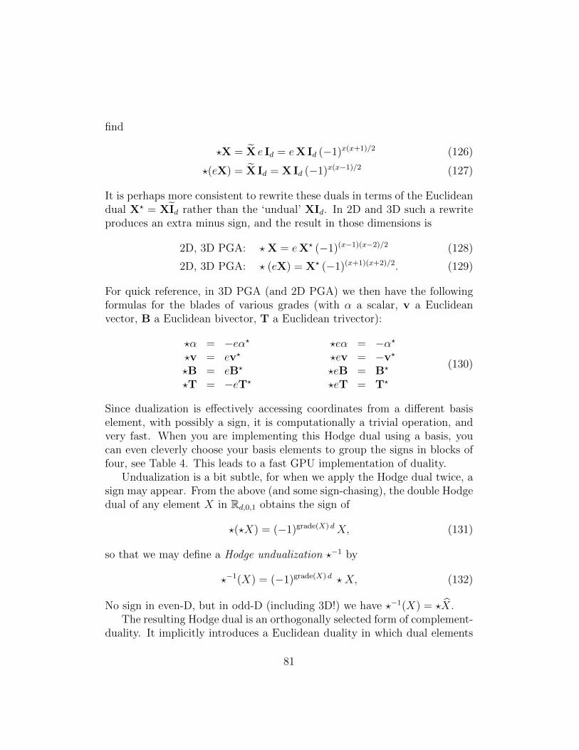
find
?X = X e Id = eX Id (−1)x(x+1)/2 (126)
?(eX) = X Id = X Id (−1)x(x−1)/2 (127)
It is perhaps more consistent to rewrite these duals in terms of the Euclideandual X? = XId rather than the ‘undual’ XId. In 2D and 3D such a rewriteproduces an extra minus sign, and the result in those dimensions is
2D, 3D PGA: ?X = eX? (−1)(x−1)(x−2)/2 (128)
2D, 3D PGA: ? (eX) = X? (−1)(x+1)(x+2)/2. (129)
For quick reference, in 3D PGA (and 2D PGA) we then have the followingformulas for the blades of various grades (with α a scalar, v a Euclideanvector, B a Euclidean bivector, T a Euclidean trivector):
?α = −eα? ?eα = −α??v = ev? ?ev = −v?
?B = eB? ?eB = B?
?T = −eT? ?eT = T?
(130)
Since dualization is effectively accessing coordinates from a different basiselement, with possibly a sign, it is computationally a trivial operation, andvery fast. When you are implementing this Hodge dual using a basis, youcan even cleverly choose your basis elements to group the signs in blocks offour, see Table 4. This leads to a fast GPU implementation of duality.
Undualization is a bit subtle, for when we apply the Hodge dual twice, asign may appear. From the above (and some sign-chasing), the double Hodgedual of any element X in Rd,0,1 obtains the sign of
?(?X) = (−1)grade(X) dX, (131)
so that we may define a Hodge undualization ?−1 by
?−1(X) = (−1)grade(X) d ? X, (132)
No sign in even-D, but in odd-D (including 3D!) we have ?−1(X) = ?X.The resulting Hodge dual is an orthogonally selected form of complement-
duality. It implicitly introduces a Euclidean duality in which dual elements
81
?1 = e0123 ?e0123 = 1?e0 = e123 ?e123 = −e0
?e1 = e032 ?e032 = −e1
?e2 = e013 ?e013 = −e2
?e3 = e021 ?e021 = −e3
?e01 = e23 ?e23 = e01
?e02 = e31 ?e31 = e02
?e03 = e12 ?e12 = e03
Table 4: Complement-duality (the Hodge star) on the basis blades of 3D PGArelative to pseudoscalar I = e ∧ e1 ∧ e2 ∧ e3 ≡ e0123. The particular basiselements are chosen to make sign patterns as symmetric as possible in blocksof 4, to enable fast implementation using standard 4D computer graphicsGPU hardware. Dualization simply becomes transfer of coordinates to a dualbasis.
are indeed orthogonal in the usual sense. Defining a Hodge dual is just a dif-ferent (and rather implicit) way of defining a metric. In fact, Browne [8] in-troduces the basic operations in the order: meet then join then complement-duality then interior product based on the complement. In this way, he endsup with a Euclidean dot product in what started as a metric-free Grassmannalgebra, getting rather close to geometric algebra at the end of his Volume1.17
I have chosen here for the order: meet, metric complement, then join interms of Euclidean complement. This approach no longer appears to need anon-Euclidean form of duality explicitly - though in an essentially projectiveapproach that motivates PGA (partly), projective duality between pointsand (hyper-)planes always has a barely hidden presence, and can be a sourceof inspiration.
9.2 The Join by Hodge Duals
We derived the join and its signs from a careful consideration of the externaldual space of PGA in Section 3.2. Having an ‘internal’ form of duality (theHodge dual) suggests that we might be able to write the join in PGA rather
17For those interested, an external appendix [9] connects our text to that of Browne’sGrassmann Algebra approach.
82
more simply. And indeed, by carefully chasing the signs of the Hodge duals,we can show that
A ∨B = ?−1(?B ∧ ?A). (133)
Note the swapping of the arguments! The proof may be found in exer-cise 12.2:12.
When you implement the Hodge dual as the coordinate manipulationindicated above, this dual outer product formula for the join leads to thefastest code. In ganja, the join is implemented in this manner at compiletime, as one of the basic operations of PGA.
Example: Hodge-based join of two points.With P = I3 + ep I3 and Q = I3 + eq2 I3, we find ?P = −e+ pand ?Q = −e+ q. Then
P ∨Q = ?−1(?Q ∧ ?P )
= ?(?Q ∧ ?P )
= ?(e(q− p) + q ∧ p
)= −(q− p)? + e(q ∧ p)?
= (q− p) I3 + e (p ∧ q) I3. (134)
This indeed agrees with the computation of this join P ∨ Q ineq.(37).
9.3 Summary
Duality is a fundamental aspect of the geometry of flats (planes, lines, points).In PGA it is more awkward than we are used to in more balanced geometricalgebras.
We tried to navigate this lightly. Our main goal was to stay within thebasic algebra Rd,0,1, since for 3D Euclidean geometry that is 4D and matchescurrent GPUs well. We showed how the Hodge dual is a workable form ofduality under these constraints, even leading to a compact and cheap join
formula eq.(133).A clever choice of basis elements for PGA, in which all signs change in
blocks of four, enables fast computation with duals (see Table 4).
83
10 Performance Considerations
(This section was contributed by Steven De Keninck.)
10.1 PGA versus CGA
Having to take the dual view (with the vectors representing planes, notpoints) and possessing a non-invertible pseudoscalar: these were both hur-dles that kept the GA community from accepting PGA for about 10 years.As we have tried to show in this replacement Chapter 11 for [1], the formeris only a conceptual issue, and the latter hardly surfaces (and where it does,it is not a programming issue, just one of algebraic purity). CGA still hasthe advantage over PGA of representing round elements like spheres, circlesand tangents as blades. But traditional graphics algorithms use the flats(planes, lines, directions), and for them PGA is a sufficiently natural envi-ronment. We have tried to convince the practitioners to use CGA for years;only in robotics, where the sphere computations really simplify the inversekinematics, has CGA gained some ground.
If flats are indeed enough in your application, the ‘1-up’ PGA is your alge-bra. And then there is a significant advantage in computational performancein not using the ‘2-up’ CGA.
• For the geometric product of a full 3D PGA multivector (from R3,0,1),192 multiplications and 176 additions are required.
• For the geometric product of a full 3D CGA multivector (from R4,1),1024 multiplications and 992 additions are required.
This makes PGA more than 5 times faster compared to CGA, for a generalgeometric product. But we should say that one rarely needs to compute a fullgeometric product of general multivectors, since sensible geometric elementsare blades or versors; still, it indicates that there is a significant difference.
10.2 PGA versus LA
However, for applications in computer graphics, the crucial comparison tomake is between PGA and the classic matrix/vector techniques from lin-ear algebra (LA). PGA builds on the representations (homogeneous points,
84
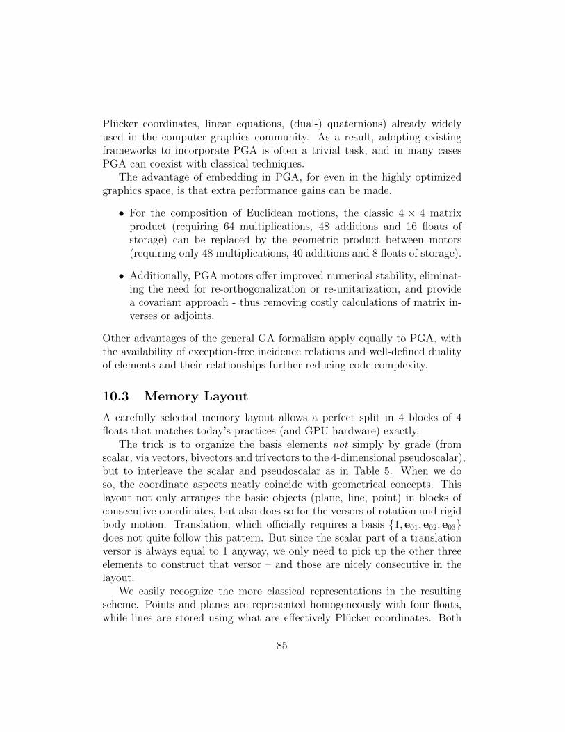
Plucker coordinates, linear equations, (dual-) quaternions) already widelyused in the computer graphics community. As a result, adopting existingframeworks to incorporate PGA is often a trivial task, and in many casesPGA can coexist with classical techniques.
The advantage of embedding in PGA, for even in the highly optimizedgraphics space, is that extra performance gains can be made.
• For the composition of Euclidean motions, the classic 4 × 4 matrixproduct (requiring 64 multiplications, 48 additions and 16 floats ofstorage) can be replaced by the geometric product between motors(requiring only 48 multiplications, 40 additions and 8 floats of storage).
• Additionally, PGA motors offer improved numerical stability, eliminat-ing the need for re-orthogonalization or re-unitarization, and providea covariant approach - thus removing costly calculations of matrix in-verses or adjoints.
Other advantages of the general GA formalism apply equally to PGA, withthe availability of exception-free incidence relations and well-defined dualityof elements and their relationships further reducing code complexity.
10.3 Memory Layout
A carefully selected memory layout allows a perfect split in 4 blocks of 4floats that matches today’s practices (and GPU hardware) exactly.
The trick is to organize the basis elements not simply by grade (fromscalar, via vectors, bivectors and trivectors to the 4-dimensional pseudoscalar),but to interleave the scalar and pseudoscalar as in Table 5. When we doso, the coordinate aspects neatly coincide with geometrical concepts. Thislayout not only arranges the basic objects (plane, line, point) in blocks ofconsecutive coordinates, but also does so for the versors of rotation and rigidbody motion. Translation, which officially requires a basis {1, e01, e02, e03}does not quite follow this pattern. But since the scalar part of a translationversor is always equal to 1 anyway, we only need to pick up the other threeelements to construct that versor – and those are nicely consecutive in thelayout.
We easily recognize the more classical representations in the resultingscheme. Points and planes are represented homogeneously with four floats,while lines are stored using what are effectively Plucker coordinates. Both
85
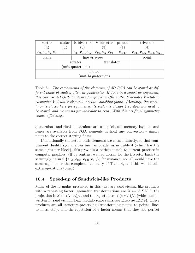
vector scalar E-bivector V-bivector pseudo trivector(4) (1) (3) (3) (1) (4)
e0, e1, e2, e3 1 e23, e31, e12 e01, e02, e03 e0123 e123, e032, e013, e021
plane line or screw pointrotator translator
(unit quaternion)motor
(unit biquaternion)
Table 5: The components of the elements of 3D PGA can be stored as dif-ferent kinds of blades, often in quadruples. If done in a smart arrangement,this can use 4D GPU hardware for graphics efficiently. E denotes Euclideanelements; V denotes elements on the vanishing plane. (Actually, the trans-lator is placed here for symmetry, its scalar is always 1 so does not need tobe stored, and we set its pseudoscalar to zero. With this artificial symmetrycomes efficiency.)
quaternions and dual quaternions are using ‘classic’ memory layouts, andhence are available from PGA elements without any conversion - simplypoint to the correct starting floats.
If additionally the actual basis elements are chosen smartly, so that com-plement duality sign changes are ‘per grade’ as in Table 4 (which has thesame signs per block), this provides a perfect match to current practice incomputer graphics. (If by contrast we had chosen for the trivector basis theseemingly natural {e123, e023, e031, e012}, for instance, not all would have thesame sign under the complement duality of Table 4, and this would takeextra operations to fix.)
10.4 Speed-up of Sandwich-like Products
Many of the formulas presented in this text are sandwiching-like productswith a repeating factor: geometric transformations are X 7→ V X V −1, theprojection is X 7→ (X ·A)/A and the rejection x 7→ (x∧A)/A (which can bewritten in sandwiching form modulo some signs, see Exercise 12.2:9). Theseproducts are all structure-preserving (transforming points to points, linesto lines, etc.), and the repetition of a factor means that they are perfect
86

candidates for symbolic optimization.Optimizing these sandwiches can often provide substantial gains (for ex-
ample, the projection of a line on a point (L · P )/P can be performed usingjust 29 multiplications compared to 42 if done fully). High performanceimplementations [18] of PGA typically include shortcuts for these commonsandwiching constructions.
10.5 Inverses
Graphics engineers to whom PGA (and GA in general) is new may be takenaback by the large number of divisions typically used in these algebras, no-tably in the sandwiching products above. However, in many cases multivectorinverses are not explicitly needed.
Even versors constructed directly as the exponential of their invariantbivectors are of the form exp(−B/2). For this kind of versor (aka a rotor),
V V = 1. Therefore their inverse is exactly equal to their reverse, which istrivial to compute: just a minus sign for the parts of grade 2 and 3.
As we already indicated in Section 6.1, for the blades and general versors,the inverse is defined as A−1 = A/(AA). In PGA, the denominator is alwayspositive (for elements for which the inverse exists at all). So if you areinterested in geometry modulo a positive scaling factor, you are allowed toreplace the inverse by the reverse. You then still retain the benefit of orientedcomputations.
For example, the projection formula (X ·A)A−1. For a normalized blade,
this is equivalent to (X · A) A which only requires the reversion operator(swapping signs of grades 2 and 3). For non-normalized blades, we can dothe same: replace the inversion by the reversion, and you may draw the result,or compute on with it, or decide to normalize it before further computations(some interpretations depend on normalization).
Normalized points, (proper) lines and planes in PGA are their own in-verses (up to a grade-dependent sign: − for point and line, + for plane). Assuch, these inversions or divisions in our cheat sheet of Table 2 do not implythe performance penalty they would in the matrix/vector approach.
87

11 To PGA! (and Beyond...)
This text intends to convey the basic structure of PGA, to help you withaccepting its rather unusual nature (yes, points are trivectors!), and to showhow things you already use (but that are somewhat extraneous to the basicLA approach, like dual quaternions) are actually fully integrated into PGA.
I hope that this write-up encourages you to try this out for yourself. Itdoes work; now make it work for you. Once you are hooked, there is no goingback; rather, you may decide to even go beyond PGA to CGA, which doesfor conformal transformations what PGA did for Euclidean motions. Themodelling principles are similar, and described in Chapters 14-16 of [1]; itis just that in CGA, spheres are the vectors, and then the rest follows. Inthis context, planes are special spheres (with infinite radius), so in ComputerScience terms CGA is a fully backwards compatible extension of PGA (seealso [5]). Mathematically, PGA is a subalgebra of CGA.
But for now, start with PGA, and enjoy!
Acknowledgement
My gratitude to Steven De Keninck, Chris Doran, Tomas Bosschieter andStephen Mann for thorough proofreading of earlier versions of this text. Anyerrors remaining have been introduced by me afterwards. Please tell meabout them at [email protected].
88

12 Exercises
12.1 Drills
1. Show that e ∧ e1 + e2 ∧ e3 is a 2-vector, but not a 2-blade. Try tofactorize it by the outer product!
2. Hail Caesar! Compute A ∨ e.
3. Show that meeting the celestial sphere (going to heaven?) reduces youto a null object: (A ∧ e)2 = 0 for all A.
4. Joining the universe will not affect you: show that I ∨A = A = A∨I.Apparently, you were already part of it...
12.2 Structural Exercises
1. Reciprocal Frames (with Section 2.2)In some of our equations, combinations of vectors occur that are mosteasily interpreted if we are aware of reciprocal frames. Let us take aside view of the two intersecting planes, used in Section 2.2 to generatethe line representation, see Figure 12.
The location of the intersection of the two lines can be found by thevertex of a parallelogram with sides parallel to the lines, and hence indirections perpendicular to n1 and n2. If we construct two vectors nr1and nr2 which satisfy n1 · nr1 = 1 and n2 · nr2 = 1 and n1 · nr2 = 0 andn2 · nr1 = 0, then we can use these as a new basis for those directionsin the plane spanned by n1 and n2. These equations show that nr1 isperpendicular to n2, with a sensibly chosen direction and length by itsrelationship to n1, and conversely for nr2, see Figure 12.
(a) Solve these equations, i.e., give expressions for nr1 and nr2.
(b) Establish the reciprocal frame relationships: the nri -coordinate ofa point x is x ·ni (and vice versa, the ni-coordinate of x is x ·nri ).
(c) Show how the reciprocal frame vectors indeed explain the posi-tional term of the line representation eq.(8). Note that this termarose automatically, so you do not actually need to know the re-ciprocal frame; it happens anyway.
89
O
nr1nr2
n1n2
p
δ2nr2
δ1nr1
δ2n2
δ1n1
Figure 12: The intersection line of two planes encoded by the reciprocal frameof their normal vectors, as seen head on in the plane spanned by their normalvectors n1 and n2. The intersection point p is most easily seen as the sumof weighted reciprocal vectors p = δ1n
r1 + δ2n
r2.
Solution: Using geometric algebra, we can easily find expressions forthe vectors nri . We compute nr1 (n1 ∧ n2) = nr1 · (n1 ∧ n2) = (nr1 ·n1) n2 − (nr1 · n2) n1 = n2, so that nr1 = n2/(n1 ∧ n2). Similarly nr2 =n1/(n2∧n1) = −n1/(n1∧n2). You can find more about these reciprocalframes in Section 3.8 of [1], such as the general form in d dimensions.For the intersection point we obtain
p = (p · n1) nr1 + (p · n2)nr2 = δ1n
r1 + δ2n
r2. (135)
We can also see this from similar triangles indicated in the figure, andrecognize these terms in eq.(8). Since Figure 12 is a perpendicular crosssection of the 3D situation, p is indeed the orthogonal support vectorof the resulting line (which sticks orthogonally out of the page), as wementioned in the main text.
2. Simplification of Expressions (with Section 2.5)Check why the following is allowed in rewriting the point representation
90

of eq.(13):
p · I3 = (p1e1 + p2e2 + p3e3) · (e1e2e3)
= p1e2e3 − p2e1e3 + p3e1e2
= p1e23 + p2e31 + p3e12. (136)
And for A purely Euclidean: eA = e ·A + e ∧A = 0 + e ∧A.
3. Point Representation in d-dimensional Space (with Section 2.5)
Show that in d dimensions, the point representation is P = (1 + ep) Id,by performing the meet of d well-chosen planes. Mind the signs!
Solution:
P =d∧i=1
(ei + (p · ei)e)
= Id +d∑i=1
e1 ∧ e2 ∧ · · · (p · ei)e ∧ · · · ∧ ed
= Id + e ∧d∑i=1
(−1)ie1 ∧ e2 ∧ · · · (p · ei) ∧ · · · ∧ ed
= Id + e ∧ (p · Id)= (1 + ep) Id. (137)
This can be interpreted as a prefix translation operator applied tothe point at the origin represented by the d-blade Id. It is in prefixform since ep anti-commutes with Id in any dimension: eId = Ide andpId = −Idp. Therefore the translation versor sandwiching productcan be rewritten in a one-sided manner: (1 + ep/2) Id(1 − ep/2) =(1 + ep/2)2 Id = (1 + ep) Id.
4. Classical Homogeneous Point Representation (Section 2.5)Show that balancing the algebra with the extra vector er reciprocal toe (so that e · er = 1), and then doing the dualization as a dot productwith the reciprocal pseudoscalar Ir ≡ e3 ∧ e2 ∧ e1 ∧ er, leads to a fairlyrecognizable form of the usual point representation p in homogeneous
91
coordinates, which would allow us to have p ·n = 0 as the homogeneousrepresentation of a plane n.
Solution: p ≡ P cIr = −p + er and p · n = −p · n + δ. Apart from asign difference, this is what you get in homogeneous coordinates.
5. The Common Factor Axiom (with Section 3.1)Using the scalar product ∗, in Chapter 3 of [1] we define the left con-traction c from the outer product ∧ by
(X ∧ A) ∗B ≡ X ∗ (AcB), for all X. (138)
It is really important to use the contraction rather than a general innerproduct for this exercise, not least because of its properties on scalars:1cB = B (rather than 0, as in some other inner products, see [19]). Wecan use this relationship to derive the Common Factor Axiom (CFA)for blades:
(B ∧ C) ∨ (A ∧B) = (A ∧B ∧ C) ∨B. (139)
This purposely has a swap of arguments relative to a similar axiom in[8], to make our join have a more pleasant semantics in the connectionof points: for us, P ∨Q is the line from P to Q. (It makes no differencewhether we put B to the left or the right on the right hand side of thisequation, see Exercise 12.1.4.)
Let grade(A ∧B ∧ C) = n, and take duality ( )∗ in that n-D space.Then we will find that the demand to have no extraneous argument-dependent signs in the CFA we should define it as:
(X ∨ Y )∗ ≡ X∗ ∧ Y ∗, (140)
or equivalently (avoiding the undualization which is so awkward todefine in degenerate spaces):
X ∨ Y ≡ X∗cY. (141)
Verify the following derivation of the CFA! (Remember that the scalarproduct is only non-zero if its two arguments have the same grade, and
92
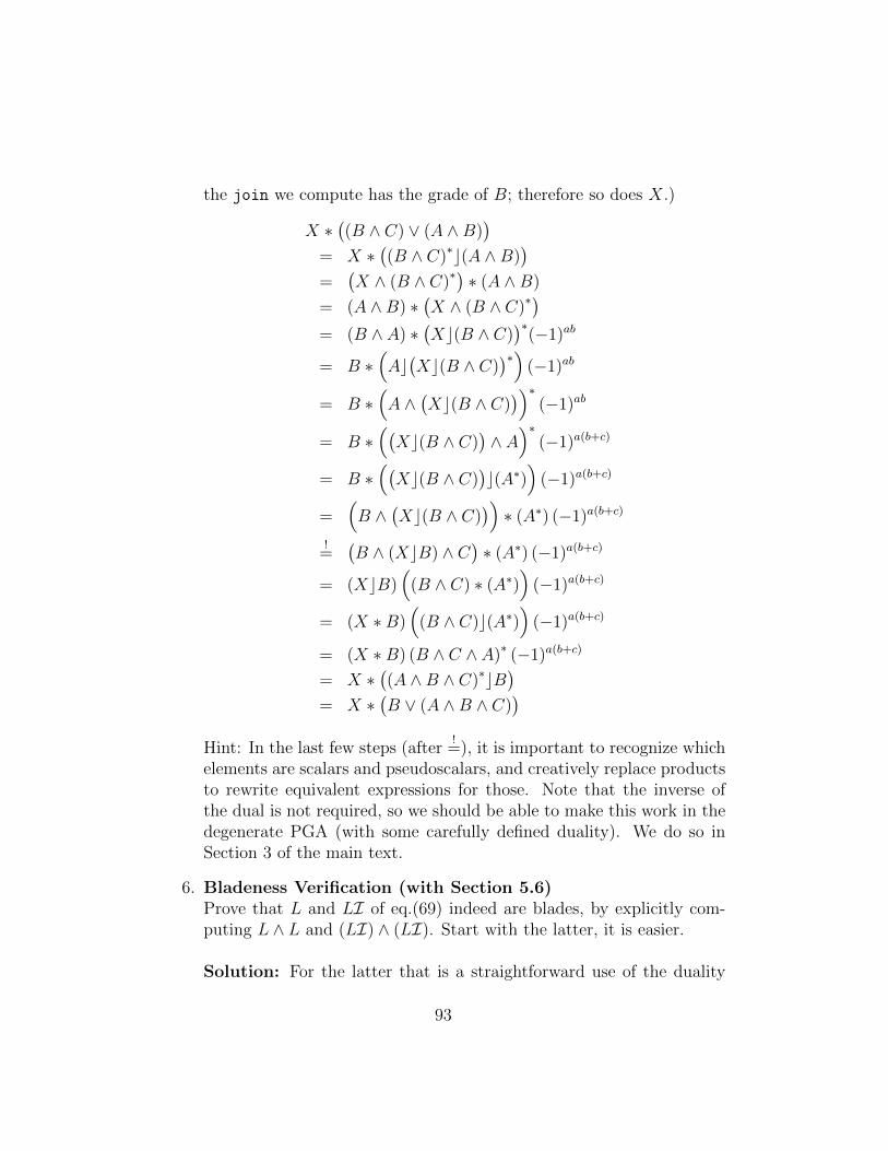
the join we compute has the grade of B; therefore so does X.)
X ∗((B ∧ C) ∨ (A ∧B)
)= X ∗
((B ∧ C)∗c(A ∧B)
)=
(X ∧ (B ∧ C)∗
)∗ (A ∧B)
= (A ∧B) ∗(X ∧ (B ∧ C)∗
)= (B ∧ A) ∗
(Xc(B ∧ C)
)∗(−1)ab
= B ∗(Ac(Xc(B ∧ C)
)∗)(−1)ab
= B ∗(A ∧
(Xc(B ∧ C)
))∗(−1)ab
= B ∗((Xc(B ∧ C)
)∧ A
)∗(−1)a(b+c)
= B ∗((Xc(B ∧ C)
)c(A∗)
)(−1)a(b+c)
=(B ∧
(Xc(B ∧ C)
))∗ (A∗) (−1)a(b+c)
!=
(B ∧ (XcB) ∧ C
)∗ (A∗) (−1)a(b+c)
= (XcB)(
(B ∧ C) ∗ (A∗))
(−1)a(b+c)
= (X ∗B)(
(B ∧ C)c(A∗))
(−1)a(b+c)
= (X ∗B) (B ∧ C ∧ A)∗ (−1)a(b+c)
= X ∗((A ∧B ∧ C)∗cB
)= X ∗
(B ∨ (A ∧B ∧ C)
)Hint: In the last few steps (after
!=), it is important to recognize which
elements are scalars and pseudoscalars, and creatively replace productsto rewrite equivalent expressions for those. Note that the inverse ofthe dual is not required, so we should be able to make this work in thedegenerate PGA (with some carefully defined duality). We do so inSection 3 of the main text.
6. Bladeness Verification (with Section 5.6)Prove that L and LI of eq.(69) indeed are blades, by explicitly com-puting L ∧ L and (LI) ∧ (LI). Start with the latter, it is easier.
Solution: For the latter that is a straightforward use of the duality
93

properties of inner and outer product :
(LI) ∧ (LI) ∝ (B I) ∧ (B I)
=(B I) ·B
)I
=(B · (B I)
)I
= (B ∧B) I2 = 0. (142)
The former is more involved. Using the symmetry of the outer productfor blades, and the fact that (B ∧B)2 = 0:
L ∧ L ∝(B (B ·B)− 1
2B(B ∧B)
)∧(B (B ·B)− 1
2B(B ∧B)
)= (B ∧B) (B ·B)2 + 1
2
(B (B ∧B)
)∧(B (B ∧B)
)−B ∧
(B (B ∧B)
)(B ·B)
= (B ∧B) (B ·B)2 + 12(B ∧B)3 − (B ·B)2 (B ∧B)
= 0. (143)
7. The Commutator of Lines (with Section 5.6)The commutator product of two 2-blades is in general a 2-vector.Therefore the commutator of two lines need not be a line. Compute it,and specify under what conditions it is a line.
Solution: (We use M to avoid some annoying signs, but this is notessential.)
L× M =(uI3 + e(p · uI3)
)×(vI3 + e(q · vI3)
)∼= u ∧ v + e
(u · (q ∧ v)− v · (p ∧ u)
)(144)
Note that this is in general not a blade, for its outer square is not zero:
(L× M) ∧ (L× M) = (u · v) e ∧ u ∧ v ∧ (p− q)
= (u · v) e ∧ u ∧ v ∧ d. (145)
Only when the lines have a point in common (which may be a vanishingpoint), or when the lines have orthogonal directions, this does equalzero.
8. Repositioning by Orthogonal Projection (with Section 5.3)Apply the projection eq.(59) on a plane n, to show its correctness in
94

that case. Then reason why that implies that it will also be correctfor all geometric primitives constructed from plane by means of meetoperations.
Solution:
(n ·X)/X =(n · ((1 + ex)I3)
)/((1 + ex)I3
)=
(n ∧ (1 + ex)
)(1− ex)
= (n− en ∧ x) (1− ex)
= n− en ∧ x + enx
= n + e (n · x). (146)
And now think ‘outermorphism’...
9. Contraction Sandwiching (with Section 5.3)We saw in Section 5.3 how to project an element onto a point, toproduce a positioning operation. You can rewrite this operation as a‘contraction sandwich’, using the left and right contraction (to show theanalogy with geometric product sandwiching when applying a versor),but this involves some extra signs. We have to use the contraction inthis exercise to make the projection universally correct in its geomet-rical meaning, even for scalars and pseudoscalars. Show that:
Tx[Ak] = (AkcX)cX−1 = (−1)k(d+1)XbAkcX−1 (147)
The two contractions in the dot sandwiching can be performed in eitherorder.
Solution: the sign difference derives from (see Section 3.4 of [1]):
XmbYn = (YncXm)∼
= (−1)n(n−1)/2+m(m−1)/2+(m−n)(m−n−1)/2XmcYn= (−1)(m+1)nXmcYn. (148)
While the dot sandwich is an interesting structural rewriting, reminis-cent of versor sandwiching, the projection formulation is more easilyremembered (it avoids the awkward sign factor). Also, it is more obvi-ously idempotent.
95

10. Translator as a Ratio of Points (with Section 6.3)Show that the ratio of two similarly weighted points Q and P gives atranslator over twice their distance.
Solution:((1+eq)I3
)/((1+ep)I3
)= (1+eq)(1−ep) = 1+e(q−p).
The actual translator is then the square root of this, which is 1 + e(q−p)/2.
11. Exact Line Correspondence Algorithm (with Section 6.8)Design an algorithm using the basic ideas of Section 6.8 to find themotor that aligns the minimum number of line correspondences in 3D.Your first step aligns the first set of lines; what are the remaining de-grees of freedom? How would you construct the next ratio of primitivesto disambiguate those while preserving the first alignment?
12. Hodge Dual Join in d Dimensions (with Section 9.2)Compute the sign in a PGA dor d-dimensional space (so Rd,0,1) relatingA ∨B to ?(?A ∧ ?B), to generalize eq.(133).
Solution: Let the pseudoscalar be e Id. We employ the Hodge du-alization equations eq.(126) and eq.(127). Then we compute the termsinvolving PA, of grade (a− 1), and PB, of grade (b− 1), in ?A and ?B.They are
PA Id (−1)(a−1)(a−2)/2 and PB Id (−1)(b−1)(b−2)/2. (149)
These are wedged together to produce a Euclidean element, and thenthe last Hodge dual produces a term of the form (modulo sign)
e((PAId) ∧ (PBId)
)Id = e
(PA
? ∧PB?)Id. (150)
which according to eq.(34) should be without a nett sign.. When wecompute its actual sign after the final Hodge, we find that it equals theparity of d + (a − 1)(b − 1). The other terms in the join turn out tobe similar in sign, so we have found in Rd,0,1:
A ∨B = ?(?A ∧ ?B) (−1)d+(a−1)(b−1)
= ?(?B ∧ ?A) (−1)d (a+b) (151)
= ?−1(?B ∧ ?A). (152)
96

By swapping the order of the arguments we have absorbed the signs ina more memorable manner. The final rewrite makes the result indepen-dent of dimension, by using the Hodge undualization of eq.(132). If youplan to work only in 3D, you could use eq.(151) in the odd-dimensional
form A ∨B = ?(?B ∧ ?A).
97

References
[1] L. Dorst, D. Fontijne, and S. Mann, Geometric Algebra for ComputerScience: An Object-oriented Approach to Geometry. Morgan Kaufman,2009. [Online]. Available: http://www.geometricalgebra.net
[2] J. M. Selig, “Clifford algebra of points, lines and planes,”Robotica, vol. 18, pp. 545–556, 2000. [Online]. Available: https://openresearch.lsbu.ac.uk/item/87v54
[3] L. Dorst, “3D oriented projective geometry through versors ofR3,3,” Advances in Applied Clifford Algebras, vol. 26, pp. 1137–1172,2016. [Online]. Available: https://link.springer.com/article/10.1007/s00006-015-0625-y
[4] S. Breuils, V. Nozick, A. Sugimoto, and E. Hitzer, “Quadric conformalgeometric algebra in R(9, 6),” Adv. Appl. Clifford Algebras, vol. 28,2018. [Online]. Available: https://link.springer.com/article/10.1007/s00006-018-0851-1
[5] C. Doran, “Euclidean geometry and geometric algebra,”June 2020, blogpost //geometry.mrao.cam.ac.uk/2020/06/euclidean-geometry-and-geometric-algebra/.
[6] S. De Keninck and L. Dorst, “Geometric Algebra Levenberg-Marquardt,” in Advances in Computer Graphics, M. Gavrilova,J. Chang, N. Thalmann, E. Hitzer, and H. Ishikawa, Eds.Cham: Springer International Publishing, 2019, pp. 511–522. [Online]. Available: https://www.springerprofessional.de/en/geometric-algebra-levenberg-marquardt/16798234
[7] ——, “Hyperwedge,” 2020, (submitted to ENGAGE 2020).
[8] J. Browne, Grassmann Algebra. Volume 1: Foundations. BarnardPublishing, 2012. [Online]. Available: https://grassmannalgebra.com/
[9] L. Dorst, “Notational correspondence between Browne’s “Grassmannalgebra” and “PGA: Plane-based geometric algebra”,” 2020, appendicalnote on bivector.net.
98

[10] S. De Keninck and C. G. Gunn, “PGA cheat sheets for the SIG-GRAPH 2019 course: 3DPGA.pdf and 2dpga.pdf,” to be found athttps://bivector.net/.
[11] S. De Keninck and L. Dorst, “PGA: clean up your mesh! (workingtitle),” 2020, in preparation.
[12] C. Gunn, “Geometry, kinematics, and rigid body mechanics inCayley-Klein geometries,” Ph.D. dissertation, TUBerlin, 2011. [Online].Available: http://page.math.tu-berlin.de/∼gunn/Documents/Papers/Thesis-final.pdf
[13] L. Dorst and R. Valkenburg, “Square root and logarithm of rotorsin 3D conformal geometric algebra using polar decomposition,”in Guide to Geometric in Practice, L. Dorst and J. Lasenby,Eds. Springer-Verlag, 2011, pp. 81–104. [Online]. Available: https://www.springer.com/gp/book/9780857298102
[14] E. Hitzer and D. Ichikawa, “Representation of crystallographicsubperiodic groups in Clifford’s geometric algebra,” Adv. Appl.Clifford Algebras, vol. 23, pp. 887–906, 2013. [Online]. Available:https://link.springer.com/article/10.1007/s00006-013-0404-6
[15] D. Fontijne and L. Dorst, “Reconstructing rotations and rigidbody motions from exact point correspondences through reflections,”in Guide to Geometric in Practice, L. Dorst and J. Lasenby,Eds. Springer-Verlag, 2011, pp. 63–78. [Online]. Available: https://www.springer.com/gp/book/9780857298102
[16] C. Doran, D. Hestenes, F. Sommen, and N. Van Acker, “Lie groupsas spin groups,” J. Math. Phys., vol. 34, no. 8, pp. 3642–3669, 1993.[Online]. Available: https://aip.scitation.org/doi/10.1063/1.530050
[17] J. Stolfi, Oriented Projective Geometry. Academic Press, 1991.
[18] J. Ong, “jeremyong/klein: v2.2.1,” March 2020, with Steven De Keninckand Faaux. [Online]. Available: https://zenodo.org/record/3711285
[19] L. Dorst, “The inner products of geometric algebra,” in Applicationsof Geometric Algebra in Computer Science and Engineering, L. Dorst,C. Doran, and L. Lasenby, Eds. Boston: Birkhauser, 2002, pp.
99

35–46. [Online]. Available: https://link.springer.com/chapter/10.1007/978-1-4612-0089-5 2
100

Index
Rd,0,1, 7c (left) contraction, 92 grade involution, 28˜ reversion, 18? Hodge dual, 80
area, 34aspect
positional, 15, 27tangential, 15, 27
bivector, 45split, 46, 47, 70
blade, 14sums of, 45
Cartan-Dieudonne, 8, 50, 58Cayley table, 32CFA, 25CGA, 6, 84, 88Chasles’theorem, 58, 67Chasles’ theorem, 50chirality, 72, 77Common Factor Axiom, 25, 92contraction, 95Cramer’s rule, 23
decomposition, 39, 47distance (oriented), 20dual
complement, 79Hodge ?, 33, 80Hodge undual ?−1, 81space, 79
example
bivector split, 47chirality, 77decomposition, 44join, 29, 83linear equations, 23motor reconstruction, 62motors, 60norm usage, 34tricycle, 67vanishing plane, 44wedge game, 23
exponentiation, 65
ganja, 10, 63
Hodge dual ?, 80
length (contour), 34line
PGA 2-blade, 15equation, 21vanishing, 17, 46, 58, 66, 67
linear algebra, 84solving equations, 23
motor, 58interpolation, 60logarithm, 71screw, 67simple, 60square root, 59tricycle, 67
norm, 32ideal, 33vanishing, 33
101

null vector, 7, 12
ordering, 72outermophism, 41
Plucker coordinates, 17, 29plane
PGA vector, 12bundle, 36, 37homogeneous equation, 11ideal, 13pencil, 43through point, 20vanishing, 13vector equation, 11
pointPGA trivector, 18, 36, 37centroid, 22on plane, 20reflection, 57vanishing, 19, 29, 68
productcommutator, 45, 94contraction, 92dot, 13geometric, 40join, 25, 27, 28, 83outer, 14regressive, 25, 27sandwich, 51, 65, 86versor, 65
projection, 37pseudoscalar
PGA, 20, 27Euclidean, 16
quaternion, 56, 64, 86dual, 50, 56, 59, 86
reciprocal frame, 15, 27, 30, 89, 90reflection, 50, 52rejection, 39repositioning, 42, 94rotation, 56rotor, 65
sandwiching, 51, 95screw
bivector, 59, 67motion, 50
translation, 55, 96
vectordirection, 19normal, 75, 76
versor, 8, 51even, 65
volume, 34
102