a hierarchal planning framework for auv mission management … · a hierarchal planning framework...
TRANSCRIPT
A Hierarchal Planning Framework for AUV Mission Management in a
Spatio-Temporal Varying Ocean
Somaiyeh MahmoudZadeh, David M.W Powers, Karl Sammut, Adham Atyabi, Amir Mehdi Yazdani
Centre for Maritime Engineering, Control and Imaging,
School of Computer Science, Engineering and Mathematics, Flinders University, Adelaide, SA, Australia
[email protected] [email protected]
Corresponding author:
Somaiyeh MahmoudZadeh
School of Computer Science, Engineering and Mathematics, Flinders University, Tonsley Park
SA 5042, Australia
E-mail: [email protected]
A Hierarchal Planning Framework for AUV Mission Management in a
Spatio-Temporal Varying Ocean
Abstract- The purpose of this paper is to provide a hierarchical dynamic mission planning framework for a single autonomous
underwater vehicle (AUV) to accomplish task-assign process in a limited time interval while operating in an uncertain undersea
environment, where spatio-temporal variability of the operating field is taken into account. To this end, a high level reactive
mission planner and a low level motion planning system are constructed. The high level system is responsible for task priority
assignment and guiding the vehicle toward a target of interest considering on-time termination of the mission. The lower layer
is in charge of generating optimal trajectories based on sequence of tasks and dynamicity of operating terrain. The mission
planner is able to reactively re-arrange the tasks based on mission/terrain updates while the low level planner is capable of coping
unexpected changes of the terrain by correcting the old path and re-generating a new trajectory. As a result, the vehicle is able
to undertake the maximum number of tasks with certain degree of maneuverability having situational awareness of the operating
field. The computational engine of the mentioned framework is based on the biogeography based optimization (BBO) algorithm
that is capable of providing efficient solutions. To evaluate the performance of the proposed framework, firstly, a realistic model
of undersea environment is provided based on realistic map data, and then several scenarios, treated as real experiments, are
designed through the simulation study. Additionally, to show the robustness and reliability of the framework, Monte-Carlo
simulation is carried out and statistical analysis is performed. The results of simulations indicate the significant potential of the
two-level hierarchical mission planning system in mission success and its applicability for real-time implementation.
Keywords- mission planning, optimization, autonomous underwater vehicle, autonomy, dynamic current, spatio-temporal ocean
Autonomous operation of AUVs in a vast, unfamiliar and dynamic underwater environment is a complicated process, especially
when the AUV is obligated to react to environment changes, where usually a-priory information is not available. Recent
advancements in sensor technology and embedded computer systems has opened new possibilities in underwater path planning
and made AUVs more capable for handling complicated long range underwater missions. However, there still exist major
challenges for this class of the vehicle, where the surrounding environment has a complex spatio-temporal variability and
uncertainty. Ocean current variability affect vehicle’s motion, for example it can perturb its safety by pushing that to an undesired
direction [1]. Consequently, this variability can also have a profound impact on vehicle’s battery usage and its mission duration.
The robustness of a vehicle’s path planning to this strong environment variability is a key element to its safety and mission
performance. Thus, robustness of the trajectory planning to current variability and terrain uncertainties is essential to mission
success and AUV safe deployment. On the other hand, an AUV should carry out complex tasks in a limited time interval.
However, existing AUVs have limited battery capacity and restricted endurance, so they should be capable of managing mission
time. Obviously, a single AUV is not able to meet all specified tasks in a single mission with limited time and energy, so the
vehicle has to effectively manage its resources to perform effective persistent deployment in longer missions without human
interaction. In this respect, time management is a fundamental requirement toward mission success that tightly depends on the
optimality of the selected tasks between start and destination point in a graph-like operation terrain. Hereupon, design of an
efficient mission planning framework considering vehicle’s availabilities and capabilities is essential requirement for
maximizing mission productivity. Many efforts have been devoted in recent years for enhancing an AUV’s capability in robust
motion planning and efficient task assignment. Although some improvement have been achieved in other autonomous systems;
there are still many challenges to achieve a satisfactory level of intelligence and robustness for AUV in this regard.
AUVs capabilities in handling mission objectives are directly influenced by routing and task arrangement system performance.
Effective routing has a great impact on a vehicle’s time management as well as mission performance by appropriate selection
and arrangement of the tasks sequence. Many attempts have been carried out in scope of single or multiple vehicles routing for
different purposes. Route planning problems usually is referred as finding shortest paths in a graph-like network such as
modelling the transportation network [2,3]. The main issue that should be covered by route planning system is to direct vehicle(s)
to its destination in a network while providing efficient maneuver and optimizing travel time. Route planning on multi-agent
decisions is implemented by Dominik et al., for the purpose of transport planning, where the agent decides between distributing
orders to customers, traversing edges, competing vendors, increasing production, etc [4]. Zou et al., investigated application of
Genetic Algorithm (GA) in dynamic route guidance system [5]. A behavior-based controller coupled with waypoint tracking
scheme is introduced by Karimanzira et al., for AUV guidance in large-scale underwater environment [6]. An integrated mission
assignment and routing strategy is proposed in [7] to serve the AUVs routing problem in order to deliver customized sensor
packages to mission targets at scattered positions, while minimising total energy cost in the presence of ocean currents. The AUV
routing problem is investigated with a Double Traveling Salesman Problem with Multiple Stacks (DTSPMS) for a single-vehicle
pickup-and-delivery problem by minimizing the total routing cost [8]. A large scale route planning and task assignment joint
problem related to the AUV activity has been investigated in [9] by transforming the problem space into a NP-hard graph context
and using the heuristic search nature of Genetic Algorithm (GA) and Particle Swarm Optimization (PSO) to find the best
waypoints. Later on, the same concept is extended by M.Zadeh et al., to AUV routing in a semi dynamic network, while
performance of the BBO and PSO algorithm is tested on single vehicle’s routing approach [10]. The real-time performance of
the application is usually overshadowed by growth of the graph complexity or problem search space. Growth of the search space
increases the computational burden that is often a problematic issue with deterministic methods such as mixed integer linear
programming (MILP) proposed by Yilmaz et al., for governing multiple AUVs [11]. In terms of task assignment, many typical
AUV missions are limited to executing a list of pre-programmed instructions and completing a predefined sequences of tasks.
The majority of the mentioned research particularly focuses on task and target assignment and time scheduling problems without
considering requirements for vehicle’s safe deployment or quality of its motion in presence of environmental disturbances. A
vehicle’s safe and confident deployment is a critical issue that should be taken into consideration at all stages of the mission in
a vast and uncertain environment. In the rest of this section, existing AUV trajectory/path planning approaches are discussed,
which are more concentrated on vehicles deployment encountering dynamicity of the operating environment
Various strategies have been developed and applied to the AUV path-planning problem in recent years. The well-known direct
method of optimal control theory, called inverse dynamics in the virtual domain (IDVD) method, was employed to develop and
test a real-time trajectory generator for realization on board of an AUV [12,13]. Willms and Yang proposed a real-time collision-
free robot path planning based on a dynamic-programming shortest path algorithm [14]. A sliding wave front expansion
algorithm applying continuous optimization techniques has been presented by Soulignac for AUVs path planning in presence of
strong current fields [15]. Jan et al., investigated higher geometry maze routing algorithm for optimal path planning and
navigating a mobile rectangular robot among obstacles [16]. Nevertheless, this strategy may not be appropriate for AUV dynamic
environments where the current field changes continuously during the mission. Earlier proposed methods [14,16] are capable of
providing optimum path planning for AUV using previous information for replanning process, which is computationally
reasonable in generating accurate local trajectories; however, they modelled the environment as a 2D space, which is inefficient
for application of the AUVs, as a 2D representation of a marine environment doesn’t sufficiently embody all the information of
a 3D ocean environment and the vehicle’s six degree of freedom. The evolution-based strategies like Differential Evolution (DE)
[17], GA [18,19] and PSO [20] are another approach that has been applied successfully to the path planning problem and are fast
enough to satisfy time restrictions of the real-time applications. A real-time online evolution based path planner was developed
for AUV rendezvous path planning in a cluttered variable environment, in which the performance of four evolutionary algorithms
of Firefly Algorithm (FA), BBO, DE, and PSO is tested and compared in different scenarios [21]. A Quantum-based PSO (QPSO)
was applied by Fu et al., for unmanned aerial vehicle’s path planning, in which only the off-line path planning in a static known
environment was implemented, which is not enough to cover dynamicity of the underwater environment [22]. Later on, this
algorithm was employed by Zeng et al., for AUV’s on-line path planning in dynamic marine environment [1].
Although various path planning techniques have been suggested for autonomous vehicles, AUV-oriented applications still have
several difficulties when operating across a large-scale geographical area. The recent investigations on path planning that
incorporate variability of the environment have assumed that planning is carried out with perfect knowledge of probable future
changes of the environment [23,24], while in the reality, accurate prediction of the environmental events such as currents or
obstacles state variations is impractical specially in longer operations. Even though available ocean predictive approaches operate
reasonably well in small scales and over short time periods, they produce insufficient accuracy to current prediction over long
time periods in larger scales, specifically in cases with lower information resolution [25]. Moreover, current variations over time
can affect moving obstacles (or waypoints in some cases) and drift them across a vehicle’s trajectory; therefore, the planned
trajectory may change and become invalid or inefficient. Proper estimation of the events in such a dynamic uncertain terrain in
long range operations, outside the vehicle’s sensor coverage, is impractical and unreliable. This becomes even more challenging
in larger dimensions, when a large data load of variation of whole terrain condition should be computed repeatedly any time that
path replanting is required, which is computationally inefficient and unnecessary as only awareness of environment changes in
vicinity of the vehicle is enough.
As mentioned earlier, the path planning problem principally deals with the quality of a vehicle’s motion between two points and
it is not an appropriate strategy to carry out vehicle’s task assignment and mission timing in a graph-like terrain. On the other
hand, vehicles routing strategies are not flexible like path planning methods in terms of handling environment sudden changes,
but they give a general overview of the area that an AUV should fly through (general route), which means reducing the operation
area to smaller operating zone for vehicle’s deployment.
To satisfy the addressed challenges and to produce a reliable mission plan for a large scale time-varying underwater
environments, this paper proposes a reactive hybrid framework that comprises an efficient mission planning system combined
with real-time path planning that improves a vehicle’s ability to complete as much of its mission as possible within the time
available. Furthermore, a path planner is designed in a smaller scale to concurrently plan trajectory between waypoints included
in the task sequence. The path planner operates in the context of the mission planner in a manner to be fast enough to handle
unforeseen changes and regenerates an alternative trajectory that safely guides the vehicle through the specified waypoints with
minimum time/energy cost. A constant interaction exists between high-low level planners across small and large scale. This
paper is a continuation of previous research [26] in which the environment modeled to be more realistic comprising uncertainty
of moving/afloat objects and dynamic multiple-layered time varying ocean current; accordingly, the path planner in current study
is facilitated with dynamic re-planning capability, which have not been addressed in the previous study. The reactive hybrid
model decides whether to carry out the path re-planning or mission re-planning procedure according to the raised situation. The
path re-planning is performed to cope with dynamic changes of the operating environment over time. On the other hand, mission
re-planning is performed to manage the lost time in cases that the path planner process takes longer than expectation. The
proposed re-planning procedure in both of the mission and path planners improve the robustness and reactive ability of the AUV
to the environmental changes and enhance its performance in accurate mission timing. Both of the planners operate individually
and concurrently while sharing their information. Parallel execution of the planners speed up the computation process.
In the core of the proposed strategy, both mission planner and local path planners make use of the Biogeography-based
Optimization (BBO) algorithm. The argument for application of BBO in solving Non-deterministic Polynomial-time (NP) hard
problems is strong enough due to its remarkable competency in scaling with multi-objective and complex problems. In this
algorithm solutions of one generation are transferred to the next and never discarded but modified. This characteristic of the
BBO enhances its exploitation ability. Solving NP-hard problems is computationally challenging and currently there is no
polynomial time algorithm to handle a NP-hard problem of even moderate size. Furthermore, finding a pure optimum solution
is only possible when the environment is fully known and no uncertainty exists. The modeled underwater environment in this
paper corresponds to a highly dynamic uncertain environment. The BBO is one of the fastest meta–heuristics algorithms
introduced for solving NP-hard complex problems. Although the captured solutions do not necessarily correspond to a pure
optimal solution, controlling the computational time is more preferable in this research due to the real-time application of the
AUV operations; hence the BBO is employed to find feasible and near optimal solutions in competitive CPU time. More
importantly, the main contribution of this paper is the proposed reactive hybrid structure which reduces run time by splitting the
operation terrain to smaller zones for the path planner and also its comprehensive application for both mission management and
path planning regardless of the employed algorithm, which has not been addressed before. The proposed autonomous/reactive
system is implemented in MATLAB®2016 and its performance is statistically analyzed.
2 Mathematical Representation of the Underwater Terrain
Existence of prior information about the terrain, location of coasts and static obstacles as the forbidden zones for deployment,
position of the start, target, and waypoints in operating area promotes AUV’s capability in robust path planning. To model a
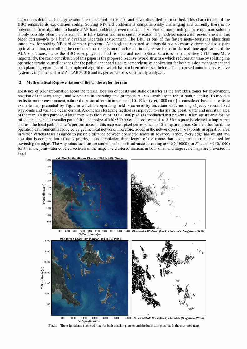
realistic marine environment, a three dimensional terrain in scale of {10×10 km (x-y), 1000 m(z)} is considered based on realistic
example map presented by Fig.1, in which the operating field is covered by uncertain static-moving objects, several fixed
waypoints and variable ocean current. A k-means clustering method is employed to classify the coast, water and uncertain area
of the map. To this purpose, a large map with the size of 1000×1000 pixels is conducted that presents 10 km square area for the
mission planner and a smaller part of the map in size of 350×350 pixels that corresponds to 3.5 km square is selected to implement
and test the local path planner’s performance. In this map each pixel corresponds to 10 m square space. On the other hand, the
operation environment is modeled by geometrical network. Therefore, nodes in the network present waypoints in operation area
in which various tasks assigned to passible distance between connected nodes in advance. Hence, every edge has weight and
cost that is combination of tasks priority, tasks completion time, length of the connection edges and the time required for
traversing the edges. The waypoints location are randomized once in advance according to ~U(0,10000) for Pix,y and ~U(0,1000)
for Piz in the joint water covered sections of the map. The clustered sections in both small and large scale maps are presented in
Fig.1.
Fig.1. The original and clustered map for both mission planner and the local path planner. In the clustered map
The clustered map is converted to a matrix format, in which the matrix size is same to map’s pixel density. The corresponding
matrix is filled with value of zero for coastal sections (forbidden area in black color), value of (0,0.35] for uncertain sections
(risky area in grey color), and value of one for water covered area as valid zone for vehicles motion that presented by white color
on the clustered map. The utilized clustering method is capable of clustering any alternative map very efficiently in a way that
the blue sections sensed as water covered zones and other sections depending on their color range categorized as forbidden and
uncertain zones.
In addition to offline map, three types of static uncertain static obstacles, afloat and self-motivated moving objects are considered
in this research to cover different possibilities of the real world situations. Movement of afloat objects are considered to be
affected by current force, where the self-motivated moving obstacles are considered to have a motivated velocity in additional
to current effects that shift them from arbitrary position A to a random direction. Obstacle’s velocity vectors and coordinates can
be measured by the sonar sensors with a specific uncertainty that modelled with a Gaussian distribution; hence, each obstacle is
presentable by its position (Θp), dimension (diameter Θr) and uncertainty ratio. Position of the obstacles initialized using normal
distribution of 𝒩�~(0,σ2) bounded to position of two targeted waypoints by the path planner (e.g. Pax,y,z<Θp<Pb
x,y,z), where σ2≈Θr.
Further detail on modeling of different obstacles can be find at [27,28].
Beside the uncertainty of operating field, which has been taken into account in the modelling the operation terrain, water current
can also have a detrimental effect on mission objectives. These issues, therefore, need to be address thoroughly in accordance
with the type and range of the mission. The ocean current information can be captured from remote observations or can be
obtained from numerical estimation models. Usually motion of the AUV is considered on the horizontal plane, because vertical
motions in ocean structure are generally negligible due to large horizontal scales comparing to vertical [29]. For the purpose of
this research, a 3D turbulent time-varying current has been applied that is generated using a multiple layered 2D current maps,
in which the current circulation patterns gradually change with depth. The current map gets updated by applying each of the
corresponding layers in a specific time step. The current map in this research modelled by:
,,,,:
),(~;0
0
)π2det(γ)(
)π(2)()(
)π(2)()(
:
)(2
)(
2
)(
0
2
)(
0
2
2
2
2
Occcc
wowc
w
wSS
SS
c
O
SS
c
O
SS
c
c
SfwvuV
SΝX
eSw
SSexxSv
SSeyySu
V
Ow
TO
O
O
(1)
In (1), the S represents a 2D space in x-y coordinates, So corresponds to the center of the turbulent, strength of the turbulent is
presented by ℑ, its radius is shown by ℓ, and λw is a covariance matrix based on radius of the turbulent. The γ is a parameter to
scale the vertical profile of the component (wc) from the horizontal components (uc,vc). For generating a dynamic ocean current
VC=(uc,vc,wc), Gaussian noise can be applied on ℓ, ℑ, and So parameters recursively, therefore we will have:
)(
0,
0
)(,
10
01
)1()(
)1()(
321
)1(21
)1(21
)1(3)1(211
tUA
tUAA
XAtAt
XAtAt
XAXASAS
CR
CR
t
t
S
tSt
ot
ot
yx
(2)
where, the current update rate in (2) is presented by URC(t) and XSx
(t-1)~𝒩(0,σSx), XSy(t-1)~𝒩(0,σSy), Xℓ
(t-1)~𝒩(0,σℓ), Xℑ(t-1)~𝒩(0,σℑ)
are Gaussian normal distributions.
3 Application of the BBO Algorithm on Mission Planning and Local Path Planning
3.1 Overview of the BBO Algorithm
The BBO is an evolutionary algorithm inspired by equilibrium theory of island biogeography concept [32] that uses the idea of
emigration, immigration, and total number of species in an island. The initial population of candidate solutions are coded with
geographically isolated islands are known as habitats. Each habitat (solution) has a quantitative performance index corresponding
to its fitness and called habitat suitability index (HSI). Respectively, the high quality habitats have higher HSI with more suitable
habitation and share their useful information with low HIS habitats. Habitability depends on qualitative factors called Suitability
Index Variables (SIVs) that is a random vector of integers. Accordingly, each habitat or candidate solution of hi possess a SIV
design variable, immigration rate (λ), and emigration rate (μ). The HSI value of each candidate solution corresponds to its fitness
that should be maximized iteratively by the algorithm based on habitat’s emigrating and immigrating features. The habitats
population should be validated by defined objective function before starting the optimization process. Poor habitats have lower
rate of emigration (μ) and higher rate immigration (λ). The SIV value of the solution hi gets probabilistically modified based on
habitats immigration rate. One of the habitats is probabilistically selected to transfer its SIV to an arbitrary solution hi according
to μ rate of the other solutions that is known as migration process in BBO. Thereupon, mutation operation is applied as a helpful
procedure to preserve diversity of the population and to steer the solutions toward the global optima. Each habitat is modified
based on probability of the existence of S species at time t in habitat hi. A habitat hi includes S species at time (t+Δt) by holding
one of the following conditions:
[1] No emigration or immigration occurred: hi includes S specie at t ⟹ hi includes S specie at (t+Δt);
[2] Immigration is occurred: hi includes S specie at t⟹ hi includes (S-1) specie at (t+Δt);
[3] Emigration is occurred: hi includes S specie at t⟹ hi includes (S+1) specie at (t+Δt);
The probability Ps(t+Δt) gives the change in number of species after time Δt, that is calculated by:
tPtPtttPttP SSSSSSSS ΔμΔλ)ΔμΔλ1)(()Δ( 1111 (3)
In (3), the λs and μs represent the immigration and emigration rates when hi holds S. As habitat suitability improves, the number
of its species and emigration increases, and the immigration rate decreases. Multiple immigration/emigration is not probable by
assuming a very small Δt; hence, the Ps is calculated as follows when Δt→0.
max11
max1111
11
μ)μ(λ
11λμ)μ(λ
0λ)μ(λ
SSPP
SSPPP
SPP
P
SSSSS
SSSSSSS
SSSSS
S (4)
In (4), Smax is the maximum species are collected in a habitat. Habitats with lower probability need to be mutated; thus, the
mutation rate m(S) for habitats has inverse relation to their probability and calculated as follows.
maxmax
1)(
P
PmSm S (5)
In (5), the mmax is the maximum mutation rate defined by user and Pmax is probability of the habitat with maximum number of
species. There are two more control parameters of maximum immigration and emigration rates for BBO process that set by the
user. Maximum emigration rate means all species are collected by a habitat. The BBO is applied in both mission planning and
path planning problem as given in two following sections.
3.2 Biogeography-based Reactive Path Planner
Robust path planning is an important characteristic of autonomy. The path planning is a NP-hard optimization problem that aims
to guide the vehicle toward a specific location encountering dynamics of the ocean and kinematics of the vehicle. An efficient
path takes the minimum travel time/distance and is safe enough to satisfy collision constraints. The path planner in this research
is capable of extracting feasible areas of a real map to determine the allowed spaces for deployment, where coastal area, islands,
static/dynamic objects and ocean current are taken into account. Water current may have positive or disturbing effect on vehicles
deployment, where an undesirable current is a disturbance itself and also it can push afloat objects across the AUV’s trajectory.
On the other hand, the desirable current can motivate AUVs motion toward its target; hence, adapting to water current variations
is an important factor affecting optimality of the generated trajectory and considerably diminish the total AUV mission costs.
The AUV is assumed to have freely deploying rigid body in 3-D space with six degrees of freedom. Six degree of freedom model
of AUV comprise translational and rotational motion [30]. The state variables corresponding to NED and Body frame are shown
by (6).
rqpwvub
ZYXn
,,,,,:}{
ψθ,φ,,,,:η}{
(6)
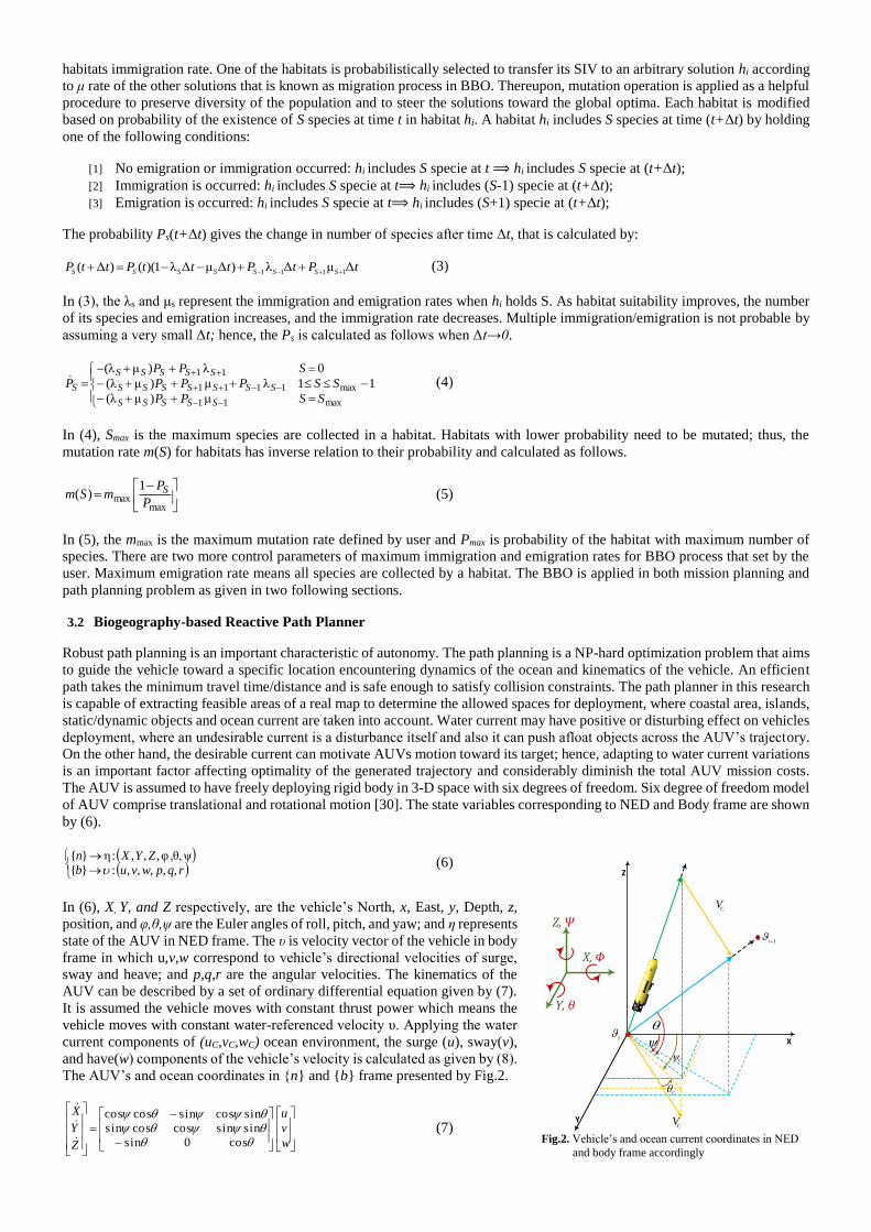
In (6), X, Y, and Z respectively, are the vehicle’s North, x, East, y, Depth, z,
position, and φ,θ,ψ are the Euler angles of roll, pitch, and yaw; and η represents
state of the AUV in NED frame. The υ is velocity vector of the vehicle in body
frame in which u,v,w correspond to vehicle’s directional velocities of surge,
sway and heave; and p,q,r are the angular velocities. The kinematics of the
AUV can be described by a set of ordinary differential equation given by (7).
It is assumed the vehicle moves with constant thrust power which means the
vehicle moves with constant water-referenced velocity υ. Applying the water
current components of (uC,vC,wC) ocean environment, the surge (u), sway(v),
and have(w) components of the vehicle’s velocity is calculated as given by (8).
The AUV’s and ocean coordinates in {n} and {b} frame presented by Fig.2.
w
v
u
Z
Y
X
cos0sin
sinsincoscossin
sincossincoscos
(7) Fig.2. Vehicle’s and ocean current coordinates in NED
and body frame accordingly
i
1i
CV
C
C
CV
Z
Y
X
Z, Ψ
X, Φ
Y, θ

CC
CCC
CCC
Vw
Vv
Vu
sinsin
sincossincos
coscoscoscos
(8)
where, the |VC| is magnitude of the current speed, ψc and θc give directions of current
vector in horizontal and vertical planes, respectively. The path curve is generated
using B-Spline method. The B-Spline curve is obtained from a sequence of control
points like ϑ= {ϑ1, ϑ2,…, ϑi,…, ϑn} that initialized in advance in the problem search
space. The mathematical description of the B-Spline coordinates is given by:
sss zyxzyx
n
iKiiz
n
iKiiy
n
iKiix
ZYX
BZ
BY
BX
,,
222,,
1,)(
1,)(
1,)(
(9)
In (9), ℘ is the generated path by B-Spline method, X,Y,Z display the vehicle’s position along the generated path. The Bi,Kis a
blending function used to slice the curve, and K is the order of the curve representing smoothness of the curve. For further
information refer to [31]. The vehicle should be oriented along the path segments generated by (9) as given by (10).
22
1
1
tan
tan
YX
Z
X
Y
(10)
Proper adjustment of these control points plays an
important role in optimality of the path curve. All control
points should be located in respective search region
constraint to predefined bounds of βiϑ=[Ui
ϑ,Liϑ]. If
ϑi:(xi,yi,zi) represent one control point in Cartesian
coordinates in tth path iteration, Liϑ is the lower bound; and
Uiϑ is the upper bound of all control points at (x-y-z)
coordinates. Fig.3 illustrates the schematic of the AUV path
planning process. In the introduced BBO based path
planner, habitat hi coded by the coordinates of the B-spline
control points and defined as a parameter to be optimized
(Ps:(h1,h2,…,hn-1)), in which the habitat’s corresponding
HSI index is presented by a randomly initialized real vector
of n-dimension. Each hi also involves a vector of n random
SIVs (hi:{ χ1, χ2,…, χn}) and approaches iteratively to its
respective best position. The mechanism of the BBO based
path planning is provided by Fig.4.
3.2.1 Path Optimization Criterion
To minimize path length/time: the path planning in this study aims to find the shortest and safest path between two
waypoints taking the advantages of desirable current while avoiding collision and adverse current fields. The AUV is
considered to have constant thrust power; therefore, the battery usage for a path is a constant function of the time and
distance travelled. Performance of the generated path is evaluated based on overall time consumption, which is proportional
to travelled distance. Assuming the constant water referenced velocity |v| for the vehicle, the travel time calculated by
1
,,
2)()1(
2)()1(
2)()1( )()()(
LT
Lsss zyx
iziziyiyixix
(11)
In (11), the L℘ and T℘ are path length and path flight time, respectively.
To satisfy path constraints: The resultant path should be safe and feasible. The environmental constraints in this paper are
associated with the forbidden zones of map, collision borders of obstacles, and current disturbance. The current disturbance
may cause drift to vehicle’s desired motion. AUV’s directional velocity components of u,v and its ψ orientation should be
constrained to umax, [vmin,vmax ], and [ψmin,ψmax], while current magnitude |Vc| and direction is encountered in all states along
Fig.3. Operation flow of the AUV path planning
Fig .4. BBO optimal path planning pseudo code
the path. The path also shouldn’t cross the forbidden collision areas
(∑M,Θ) associated with map or obstacles. The cost function defined
as a combination path time and corresponding penalty function
described in (12).
Otherwise
t
yxMapCoastt
Viol
t
vtv
utu
Viol
ViolViolfTCost
twtvtutttZtYtXt
NUrrpzyx
zyx
vu
n
i
MM
M
0
),,()(1
1),(:)(1
)(;0max(
)(;0max(
))(;0max(
,,
,
)](),(),(),(),(),(),(),([)(
,,
,,
max
max
max
1
,,
,
(12)
In (12), the γf(Viol℘, Viol∑M,Θ) is a weighted violation function that
respects AUV’S vehicular and collision constraints; γu, γv, γψ, and
γ∑M,Θ denote the impact of each violation in calculation of path cost.
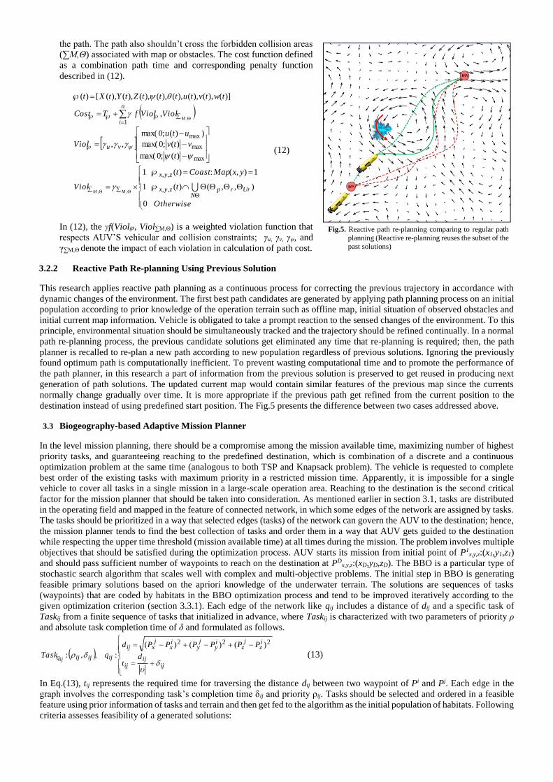
3.2.2 Reactive Path Re-planning Using Previous Solution
This research applies reactive path planning as a continuous process for correcting the previous trajectory in accordance with
dynamic changes of the environment. The first best path candidates are generated by applying path planning process on an initial
population according to prior knowledge of the operation terrain such as offline map, initial situation of observed obstacles and
initial current map information. Vehicle is obligated to take a prompt reaction to the sensed changes of the environment. To this
principle, environmental situation should be simultaneously tracked and the trajectory should be refined continually. In a normal
path re-planning process, the previous candidate solutions get eliminated any time that re-planning is required; then, the path
planner is recalled to re-plan a new path according to new population regardless of previous solutions. Ignoring the previously
found optimum path is computationally inefficient. To prevent wasting computational time and to promote the performance of
the path planner, in this research a part of information from the previous solution is preserved to get reused in producing next
generation of path solutions. The updated current map would contain similar features of the previous map since the currents
normally change gradually over time. It is more appropriate if the previous path get refined from the current position to the
destination instead of using predefined start position. The Fig.5 presents the difference between two cases addressed above.
3.3 Biogeography-based Adaptive Mission Planner
In the level mission planning, there should be a compromise among the mission available time, maximizing number of highest
priority tasks, and guaranteeing reaching to the predefined destination, which is combination of a discrete and a continuous
optimization problem at the same time (analogous to both TSP and Knapsack problem). The vehicle is requested to complete
best order of the existing tasks with maximum priority in a restricted mission time. Apparently, it is impossible for a single
vehicle to cover all tasks in a single mission in a large-scale operation area. Reaching to the destination is the second critical
factor for the mission planner that should be taken into consideration. As mentioned earlier in section 3.1, tasks are distributed
in the operating field and mapped in the feature of connected network, in which some edges of the network are assigned by tasks.
The tasks should be prioritized in a way that selected edges (tasks) of the network can govern the AUV to the destination; hence,
the mission planner tends to find the best collection of tasks and order them in a way that AUV gets guided to the destination
while respecting the upper time threshold (mission available time) at all times during the mission. The problem involves multiple
objectives that should be satisfied during the optimization process. AUV starts its mission from initial point of P1x,y,z:(x1,y1,z1)
and should pass sufficient number of waypoints to reach on the destination at PDx,y,z:(xD,yD,zD). The BBO is a particular type of
stochastic search algorithm that scales well with complex and multi-objective problems. The initial step in BBO is generating
feasible primary solutions based on the apriori knowledge of the underwater terrain. The solutions are sequences of tasks
(waypoints) that are coded by habitats in the BBO optimization process and tend to be improved iteratively according to the
given optimization criterion (section 3.3.1). Each edge of the network like qij includes a distance of dij and a specific task of
Taskij from a finite sequence of tasks that initialized in advance, where Taskij is characterized with two parameters of priority ρ
and absolute task completion time of δ and formulated as follows.
ijij
ij
iz
jz
iy
jy
ix
jxij
ijijijq dt
PPPPPPd
qTaskij
222 )()()(
:,,: (13)
In Eq.(13), tij represents the required time for traversing the distance dij between two waypoint of Pi and Pj. Each edge in the
graph involves the corresponding task’s completion time δij and priority ρij. Tasks should be selected and ordered in a feasible
feature using prior information of tasks and terrain and then get fed to the algorithm as the initial population of habitats. Following
criteria assesses feasibility of a generated solutions:
WPi
WPj
Fig.5. Reactive path re-planning comparing to regular path
planning (Reactive re-planning reuses the subset of the
past solutions)
Valid solution is a sequence of nodes that commenced
and ended with index of the predefined start and
destination points.
Valid solution does not include edges that are not
presented in the graph.
Valid solution does not include a specific node for
multiple times, as multiple appearance of the same node
implies wasting time repeating a task.
Valid solution does not traverse an edge more than once.
Valid solution has total completion time smaller than the
maximum range of mission available time.
A priority-based strategy is conducted by this research to
generate feasible solutions to the defined criteria, in which a
randomly initialized priority vector is assigned to sequence of
nodes in the graph. Adjacency information of the graph and
provided priority vector get conducted for proper node
selection. The priority vector for corresponding nodes takes
positive or negative values in the specified range of [-200,100].
Afterward, nodes are added to the sequence one by one
according to priority vector and graph adjacency relations.
Visited nodes get a large negative priority value that prevents
repeated visits them. The traversed edges of the graph get
eliminated from the adjacency matrix.
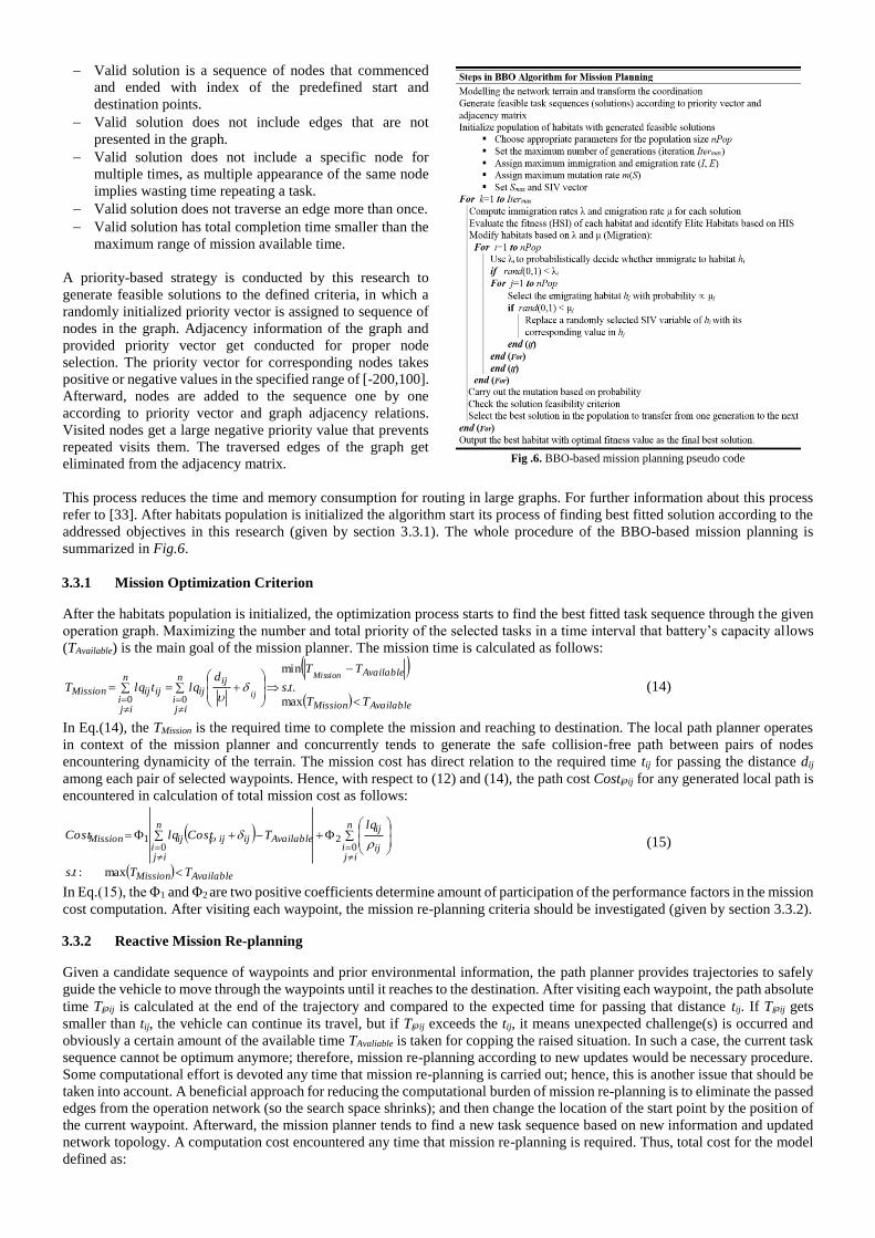
This process reduces the time and memory consumption for routing in large graphs. For further information about this process
refer to [33]. After habitats population is initialized the algorithm start its process of finding best fitted solution according to the
addressed objectives in this research (given by section 3.3.1). The whole procedure of the BBO-based mission planning is
summarized in Fig.6.
3.3.1 Mission Optimization Criterion
After the habitats population is initialized, the optimization process starts to find the best fitted task sequence through the given
operation graph. Maximizing the number and total priority of the selected tasks in a time interval that battery’s capacity allows
(TAvailable) is the main goal of the mission planner. The mission time is calculated as follows:
AvailableMission
Availablen
iji
ijij
n
iji
ijijMissionTT
ts
TTd
lqtlqTMission
ij
max
..
min
00
(14)
In Eq.(14), the TMission is the required time to complete the mission and reaching to destination. The local path planner operates
in context of the mission planner and concurrently tends to generate the safe collision-free path between pairs of nodes
encountering dynamicity of the terrain. The mission cost has direct relation to the required time tij for passing the distance dij
among each pair of selected waypoints. Hence, with respect to (12) and (14), the path cost Cost℘ij for any generated local path is
encountered in calculation of total mission cost as follows:
AvailableMission
n
iji ij
ijAvailable
n
iji
ijijijMission
TTts
lqTCostlqCost
max:.
02
01
(15)
In Eq.(15), the Φ1 and Φ2 are two positive coefficients determine amount of participation of the performance factors in the mission
cost computation. After visiting each waypoint, the mission re-planning criteria should be investigated (given by section 3.3.2).
3.3.2 Reactive Mission Re-planning
Given a candidate sequence of waypoints and prior environmental information, the path planner provides trajectories to safely
guide the vehicle to move through the waypoints until it reaches to the destination. After visiting each waypoint, the path absolute
time T℘ij is calculated at the end of the trajectory and compared to the expected time for passing that distance tij. If T℘ij gets
smaller than tij, the vehicle can continue its travel, but if T℘ij exceeds the tij, it means unexpected challenge(s) is occurred and
obviously a certain amount of the available time TAvaliable is taken for copping the raised situation. In such a case, the current task
sequence cannot be optimum anymore; therefore, mission re-planning according to new updates would be necessary procedure.
Some computational effort is devoted any time that mission re-planning is carried out; hence, this is another issue that should be
taken into account. A beneficial approach for reducing the computational burden of mission re-planning is to eliminate the passed
edges from the operation network (so the search space shrinks); and then change the location of the start point by the position of
the current waypoint. Afterward, the mission planner tends to find a new task sequence based on new information and updated
network topology. A computation cost encountered any time that mission re-planning is required. Thus, total cost for the model
defined as:
Fig .6. BBO-based mission planning pseudo code
r
computeMissionTotal TCostCost1
(16)
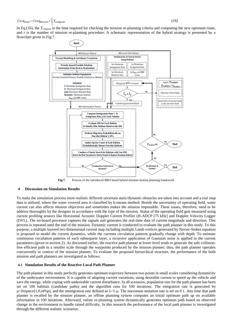
In Eq.(16), the Tcompute is the time required for checking the mission re-planning criteria and computing the new optimum route,
and r is the number of mission re-planning procedure. A schematic representation of the hybrid strategy is presented by a
flowchart given in Fig.7.
Termination Criterion IsAttained?
No Yes
Start
Terrain Modelling & Coordinate Transform
Priority-based Feasible Solution Generation From Strat to Destination
Compute Immigration Rates λ &
Emigration Rate μ for Each Solution
Initialize Habitat Population: Encode Generated Primary Feasible Solutions as Habitats
Initialize:I: Maximum Immigration Rate
E: Maximum Emigration Rate
m(S): Maximum Mutation Rate
RouteIter: Maximum Iteration
Smax and SIV vector
Evaluate HIS for Each Habitat
& Identify Elite Habitats Based on the HSI
Perform Migration Probabilistically on
Non-elite Habitat s SIVs
Update Species Count of Each Habitat.
Probabilistically Mutate Non-elite Habitats
Conduct a Chaotic Search for Habitats with Low HIS
Select the Best Parameters Newly Found to Replace Random Habitat
No
Waypoint WPi is visited
T tij
Continue generated Route
Yes
Update TAvailable
TAvailable TResidual
Eliminate Visited Edges
Send Index of Current Node as the new Start Node
Set Maximum
Immigration Rate
Set Maximum
Emigration Rate
Initialization of Control-Points
Using Habitat
BBO Local Path Planner
Set Smax and SIV
vector
Set Maximum
Mutation Rate
BBO Mission Planner
BBO Optimization Process
Destination Is Visited?
No
Yes
End
TResidual 0Yes
End
No
Fig.7. Process of the introduced BBO based hybrid mission-motion planning framework
4 Discussion on Simulation Results
To make the simulation process more realistic different uncertain static/dynamic obstacles are taken into account and a real map
data is utilized, where the water covered area is classified by k-means method. Beside the uncertainty of operating field, water
current can also affects mission objectives and sometimes makes the mission impossible. These issues, therefore, need to be
address thoroughly by the designer in accordance with the type of the mission. Status of the operating field gets measured using
current profiling sensors like Horizontal Acoustic Doppler Current Profiler (H-ADCP [75 kHz] and Doppler Velocity Logger
(DVL). The on-board processor captures the signals and generates the real-time data of current magnitude and direction. This
process is repeated until the end of the mission. Dynamic current is conducted to evaluate the path planner in this study. To this
purpose, a multiple layered two dimensional current map including multiple Lamb vortices generated by Navier-Stokes equation
is proposed to model the current dynamics, while the currents circulation patterns gradually change with depth. To estimate
continuous circulation patterns of each subsequent layer, a recursive application of Gaussian noise is applied to the current
parameters (given in section 2). As discussed earlier, the reactive path planner at lower level tends to generate the safe collision-
free efficient path in a smaller scale through the waypoints produced by the mission planner; thus, the path planner operates
concurrently in context of the mission planner. To evaluate the proposed hierarchical structure, the performance of the both
mission and path planners are investigated as follows.
4.1 Simulation Results of the Reactive Local Path Planner
The path planner in this study perfectly generates optimum trajectory between two points in small scales considering dynamicity
of the underwater environment. It is capable of adapting current variations, using desirable current to speed up the vehicle and
save the energy, while coping with undesirable current disturbance. In all scenarios, population size for the path planner has been
set on 100 habitats (candidate paths) and the algorithm runs for 100 iterations. The emigration rate is generated by
μ=linspace(1,0,nPop), and the immigration rate defined as λ=1-μ. The maximum mutation rate is set on 0.1. Any time that path
planner is recalled by the mission planner, an offline planning system computes an initial optimum path up on available
information in 100 iterations. Afterward, online re-planning system dynamically generates optimum path based on observed
change in the environment to handle raised difficulty. In this research the performance of the local path planner is investigated
through the different realistic scenarios:
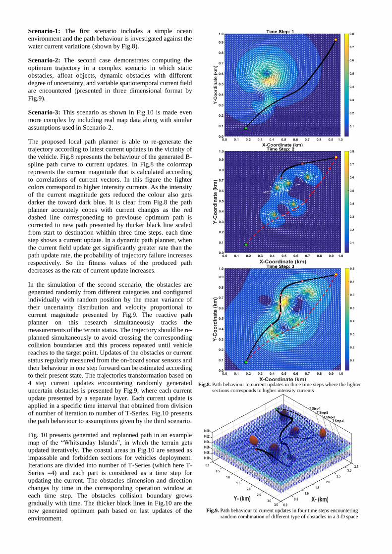
Scenario-1: The first scenario includes a simple ocean
environment and the path behaviour is investigated against the
water current variations (shown by Fig.8).
Scenario-2: The second case demonstrates computing the
optimum trajectory in a complex scenario in which static
obstacles, afloat objects, dynamic obstacles with different
degree of uncertainty, and variable spatiotemporal current field
are encountered (presented in three dimensional format by
Fig.9).
Scenario-3: This scenario as shown in Fig.10 is made even
more complex by including real map data along with similar
assumptions used in Scenario-2.
The proposed local path planner is able to re-generate the
trajectory according to latest current updates in the vicinity of
the vehicle. Fig.8 represents the behaviour of the generated B-
spline path curve to current updates. In Fig.8 the colormap
represents the current magnitude that is calculated according
to correlations of current vectors. In this figure the lighter
colors correspond to higher intensity currents. As the intensity
of the current magnitude gets reduced the colour also gets
darker the toward dark blue. It is clear from Fig.8 the path
planner accurately copes with current changes as the red
dashed line corresponeding to previouse optimum path is
corrected to new path presented by thicker black line scaled
from start to destination whithin three time steps. each time
step shows a current update. In a dynamic path planner, when
the current field update get significantly greater rate than the
path update rate, the probability of trajectory failure increases
respectively. So the fitness values of the produced path
decreases as the rate of current update increases.
In the simulation of the second scenario, the obstacles are
generated randomly from different categories and configured
individually with random position by the mean variance of
their uncertainty distribution and velocity proportional to
current magnitude presented by Fig.9. The reactive path
planner on this research simultaneously tracks the
measurements of the terrain status. The trajectory should be re-
planned simultaneously to avoid crossing the corresponding
collision boundaries and this process repeated until vehicle
reaches to the target point. Updates of the obstacles or current
status regularly measured from the on-board sonar sensors and
their behaviour in one step forward can be estimated according
to their present state. The trajectories transformation based on
4 step current updates encountering randomly generated
uncertain obstacles is presented by Fig.9, where each current
update presented by a separate layer. Each current update is
applied in a specific time interval that obtained from division
of number of iteration to number of T-Series. Fig.10 presents
the path behaviour to assumptions given by the third scenario.
Fig. 10 presents generated and replanned path in an example
map of the “Whitsunday Islands”, in which the terrain gets
updated iteratively. The coastal areas in Fig.10 are sensed as
impassable and forbidden sections for vehicles deployment.
Iterations are divided into number of T-Series (which here T-
Series =4) and each part is considered as a time step for
updating the current. The obstacles dimension and direction
changes by time in the corresponding operation window at
each time step. The obstacles collision boundary grows
gradually with time. The thicker black lines in Fig.10 are the
new generated optimum path based on last updates of the
environment.
Fig.8. Path behaviour to current updates in three time steps where the lighter
sections corresponds to higher intensity currents
Fig.9. Path behaviour to current updates in four time steps encountering
random combination of different type of obstacles in a 3-D space
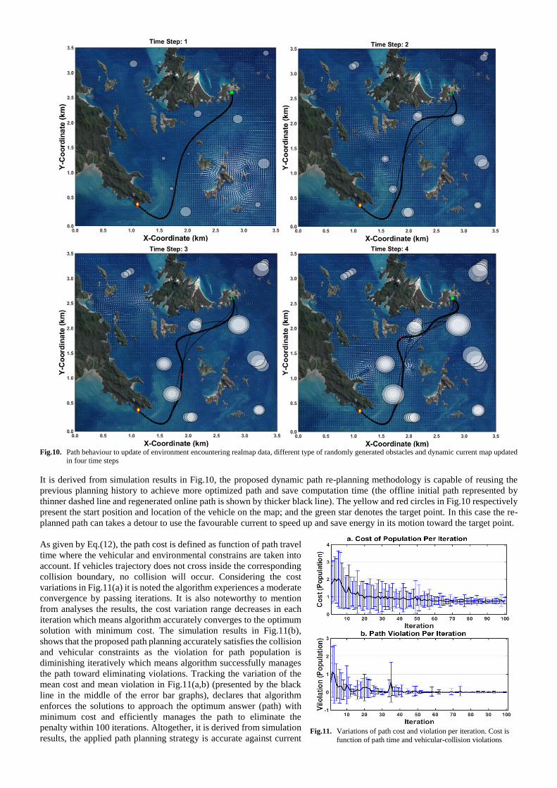
Fig.10. Path behaviour to update of environment encountering realmap data, different type of randomly generated obstacles and dynamic current map updated
in four time steps
It is derived from simulation results in Fig.10, the proposed dynamic path re-planning methodology is capable of reusing the
previous planning history to achieve more optimized path and save computation time (the offline initial path represented by
thinner dashed line and regenerated online path is shown by thicker black line). The yellow and red circles in Fig.10 respectively
present the start position and location of the vehicle on the map; and the green star denotes the target point. In this case the re-
planned path can takes a detour to use the favourable current to speed up and save energy in its motion toward the target point.
As given by Eq.(12), the path cost is defined as function of path travel
time where the vehicular and environmental constrains are taken into
account. If vehicles trajectory does not cross inside the corresponding
collision boundary, no collision will occur. Considering the cost
variations in Fig.11(a) it is noted the algorithm experiences a moderate
convergence by passing iterations. It is also noteworthy to mention
from analyses the results, the cost variation range decreases in each
iteration which means algorithm accurately converges to the optimum
solution with minimum cost. The simulation results in Fig.11(b),
shows that the proposed path planning accurately satisfies the collision
and vehicular constraints as the violation for path population is
diminishing iteratively which means algorithm successfully manages
the path toward eliminating violations. Tracking the variation of the
mean cost and mean violation in Fig.11(a,b) (presented by the black
line in the middle of the error bar graphs), declares that algorithm
enforces the solutions to approach the optimum answer (path) with
minimum cost and efficiently manages the path to eliminate the
penalty within 100 iterations. Altogether, it is derived from simulation
results, the applied path planning strategy is accurate against current
Fig.11. Variations of path cost and violation per iteration. Cost is
function of path time and vehicular-collision violations

immediate updates. Moreover, increasing the complexity of the obstacles, increases the problems complexity, however, it is
noted from simulation results in Fig.9 and Fig.10 that the algorithm is able to accurately handle the collision avoidance regardless
of type or number of appeared obstacles in all three scenarios. The trajectory is re-planned simultaneously to avoid turbulent or
crossing the corresponding collision boundaries and this process repeated until vehicle reaches to the target point. Further, it is outstanding in Fig.11 that the algorithm satisfies collision and vehicular constraint while minimizing the path cost that is
proportional to path length and time.
4.2 Simulation Results of the hierarchical reactive mission planning system
To evaluate the proposed hybrid reactive system, additional to local path planner that is evaluated above, the mission planner
and concordance of two mission-motion planners should be investigated. To this purpose, some performance metrics have been
investigated through the subsets of representative Monte Carlo simulations presented and discussed by Fig.12 to 15. The BBO,
in this circumstance, is configured with habitat population size of 150, iterations of 200, and the Monte Carlo simulations is set
on 100 runs, emigration rate, immigration rate , and maximum mutation rate are set on μ=0.2, λ=1-μ, and m(S)=0.5, respectively.
The system aims to take the maximum use of the mission available time (TAvailable), increase the mission productivity by collecting
best sequence of tasks fitted to TAvailable, guarantee on-time termination of the mission; and concurrently ensuring the vehicles
safety by copping dynamic unexpected environmental challenges during the mission. As regards, the vehicle’s safe deployment
is carried out by the local path planner. The stability of the model in time management is the most critical factor representing
robustness of the method. To this end, the robustness of the hierarchal model in enhancement of the vehicles autonomy in terms
of mission time management is evaluated by testing 100 missions’ through individual experiments with the same initial condition
that closely matches actual underwater mission scenarios and presented by Fig.12 to 15. The number of waypoints is fixed on
40 nodes for all Monte Carlo runs, but the topology of the graph is changed randomly based on a Gaussian distribution on the
problem search space. The time threshold (TAvailable) also fixed on 4 hours (14,400 seconds).
Fig.12. Performance of the model in maximizing the mission time constraint to available time threshold
To establish appropriate collaboration between the low and high level mission-motion planners, the correlation between the
expected time for passing a specific distance (tij) and the generated path time (T℘) is another important performance index
affecting concordance of the whole system that investigated and presented by Fig.13. The tij for the local planner is determined
from the estimated mission time (given by Eq.(14)).
Fig.13. Stability of the hierarchical reactive system in managing correlation between expected and path time (tij and T℘) in multiple recall of the local path
planner in each mission through the 100 Monte Carlo simulations
Fig.14. Relative proportions of CPU time used for a single run of the path planning compared to overall CPU time for mission which includes multiple
operation of the path planner.
The most appropriate outcome for a mission is completion of
the mission with the minimum residual time (TResidual), which
means maximizing the use of mission available time. The
mission time (TMission) is the summation of time taken for
passing through the waypoints (produced by the local path
planner) and completion time for covered tasks along paths.
It is clear in Fig.12 the proposed hierarchal reactive system
is capable of taking maximum use of available time as the
TMission in all experiments approaches the TAvailable and meet
the above constraints denoted by the upper bound of 14400
sec (4 hours) presented by red line. Respectively, the TResidual
that has a linear relation to TMission should be minimized but it
should not be equal to zero that is accurately satisfied
considering variations of TResidual over 100 missions.
Considering the fact that reaching to the destination is a big
concern for vehicles safety, a big penalty value is assigned to
strictly prevent missions from taking more time than TAvailable.
Existence of a reasonable correlation between T℘ and tij values in each path planning operation is critical to total
performance of the hierarchical model, which means a big
difference between these two parameters cause interruption
in cohesion of the whole system. It is derived from simulation
result in Fig.13 that variations of both T℘ and tij are lied in
similar range and very close to each other in which the T℘ and
tij are presented with yellow transparent boxplot and blue
compact boxplot, respectively.
Another highlighted factor is the computational time for
mission and path planning operations. The reason for
highlighting the CPU time is that the local planner must
operate synchronous to the mission planner; thus, a large
CPU time again causes interruption to concurrent operation
of two planners, which this issue flaws the routine flow and
cohesion of the whole system. Fig.14 presents the relative
proportions of CPU time used for a single run of the path
planning compared to overall CPU time for mission which
includes multiple operation of the path planner. It is
noteworthy to mention from analyze of the simulation results
in Fig.14 that the model takes a very short CPU time for all
experiments that makes it highly accurate for real-time
application. As the local planner operates multiple time in
context of the mission planner, obviously it takes shorter time
and lower cost, comparatively. It is evident from Fig.14 that
the range of variations of CPU time for both planners is
almost in similar range in all experiments that proves the
inherent stability of the model’s real-time performance. The
results obtained from Monte Carlo analyze (presented by
Fig12 to Fig.14) demonstrate the inherent robustness and
drastic efficiency of the proposed hierarchical reactive
system in terms of time management and increasing mission
productivity by maximizing TMission while each mission is
terminated before vehicle runs out of time/energy, as in all
experiment TResidual gets nonzero positive value.
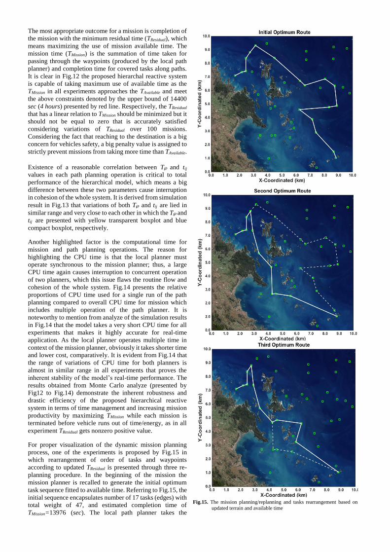
For proper visualization of the dynamic mission planning
process, one of the experiments is proposed by Fig.15 in
which rearrangement of order of tasks and waypoints
according to updated TResidual is presented through three re-
planning procedure. In the beginning of the mission the
mission planner is recalled to generate the initial optimum
task sequence fitted to available time. Referring to Fig.15, the
initial sequence encapsulates number of 17 tasks (edges) with
total weight of 47, and estimated completion time of
TMission=13976 (sec). The local path planner takes the
Fig.15. The mission planning/replanning and tasks rearrangement based on
updated terrain and available time
waypoint sequence and starts generating feasible path through the listed waypoints in the initial sequence; hence the local planner
adopts the first pair of waypoints and generate a feasible trajectory between them with time of T℘=923.2(sec) which is smaller
than expected travel time tij=987.7(sec). In cases that T℘ is smaller than tij, the mission replanting flag is zero - the initial sequence
is still valid and optimum- so the vehicle is allowed to follow the next pair of waypoints included in initial sequence. After each
run of the path planner, the path time T℘ is reduced from the TResidual. Accordingly, waypoints are shifted to the local planner and
the same process is repeated until the T℘ exceeds the tij. In this circumstance, the mission re-planning flag gets one, which means
some of the available time is wasted in passing the distance between those nodes. Hence, the TResidual gets updated and the global
planner is recalled to rearrange the tasks order and regenerate a new task sequence from the existing node. In simulation results
presented in Fig.15, the mission planner is recalled for 3 times and the local path planner is called for 11 times. This interplay
among the path planner and mission planner continues until vehicle reaches to the destination (success) or TResidual gets a minus
value (failure: vehicle runs out of battery).
5 Conclusion
A two-level dynamic mission-motion planning for AUV’s optimal task-assignment and time management has been developed.
The higher level mission planner provides the best sequence of waypoints (tasks) with respect to the mission objectives. By
doing this, the optimal deployment zone is selected and the search area is minimized. Afterward, the local reactive path planner
starts generating optimal collision-free path through the listed waypoints; copping any unexpected environmental changes is
done by correcting the old path or re-generating a new path. The spatio-temporal variability of the operating field is tracked and
then based on new situational awareness of surrounding environment the mission planner updates the tasks orders. The local
path planner in current study mainly focuses on finding the optimal trajectory by using the advantages of desirable current field
and avoiding obstacles and no-fly zones. The proposed hybrid reactive system takes advantage of the BBO algorithm on both
mission and path planners where the main objectives of the system is to have a beneficial mission, manage the mission time
considering total available time, task priority assignment, and safe deployment. Knowing the fact that existing approaches mainly
are able to cover only a part of problem of ether motion/path planning or task assignment based on offline map, the provided
framework is remarkable contribution to improve AUV’s autonomy in both higher/lower level due to its comprehensive mission-
motion planning capability that covers shortcomings associated with previous strategies used in this scope. Future work will
concentrate on the design of a modular architecture with an additional module of predictor–corrector encompassing the ability
of at least one step ahead prediction of situational awareness of the environment that results in more flexibility for successful
mission in real-world experiments.
References
[1] Zeng Z, Sammut K, Lammas A, He F, Tang Y. Shell space decomposition based path planning for AUVs operating in a variable environment. Journal of
Ocean Engineering; 2014; 91: 181-195.
[2] Geisberger R. Advanced Route Planning in Transportation Networks. (Ph.D. thesis) Karlsruhe Institute of Technology, Karlsruhe; 2011; p.1–227.
[3] Kosicek M, Tesar R, Darena F, Malo R, Motycka A. Route planning module as a part of supply chain management system. Acta Universitatis Agriculturaeet Silviculturae Mendelianae Brunensis; 2012; 2:135–142.
[4] Dominik B, Katharina S, Axel T. Multi-agent-based transport planning in the newspaper industry. International Journal of Production Economics, Elsevier;
2011; 131(1): 146–157.
[5] Zou L, Xu J, Zhu L. Application of genetic algorithm in dynamic route guidance system. Journal of Transportation Systems Engineering and Information
Technology; 2007; 7(3): 45–48.
[6] Karimanzira D, Jacobi M, Pfuetzenreuter T, Rauschenbach T, Eichhorn M, Taubert R, Ament C. First testing of an AUV mission planning and guidance system for water quality monitoring and fish behavior observation in net cage fish farming. Information Processing in Agriculture, Elsevier; 2014; 1: 131–
140.
[7] Yan W, Bai X, Peng X, Zuo L, Dai J. The Routing Problem of Autonomous Underwater Vehicles in Ocean Currents; 2014. Doi:978-1-4799-3646-5/14/2014 IEEE
[8] Iori M, Riera-Ledesma J. Exact algorithms for the double vehicle routing problem with multiple stacks. Computers & Operations Research; 2015; 63: 83–
10.
[9] MahmoudZadeh S, Powers D, Sammut K, Lammas A, Yazdani AM. Optimal Route Planning with Prioritized Task Scheduling for AUV Missions. IEEE
International Symposium on Robotics and Intelligent Sensors; 2015; p.7-15.
[10] MahmoudZadeh S, Powers D, Yazdani AM. A Novel Efficient Task-Assign Route Planning Method for AUV Guidance in a Dynamic Cluttered
Environment. IEEE Congress on Evolutionary Computation (CEC). Vancouver, Canada; July 2016; CoRR abs/1604.02524 (2016). Robotics (cs.RO). arXiv:1604.02524
[11] Yilmaz NK, Evangelinos C, Lermusiaux PFJ, Patrikalakis NM. Path planning of autonomous underwater vehicles for adaptive sampling using mixed integer
linear programming. IEEE Journal of Oceanic Engineering; 2008; 33 (4): 522–537.
[12] Yazdani AM, Sammut K, Yakimenko OA, Lammas A, MahmoudZadeh S, Tang Y. IDVD-Based Trajectory Generator for Autonomous Underwater
Docking Operations. Robotics and Autonomous Systems; 2017; 92:12–29.
[13] Yazdani AM, Sammut K, Yakimenko OA, Lammas A, MahmoudZadeh S, Tang Y. Time and energy efficient trajectory generator for autonomous underwater vehicle docking operations. In OCEANS 2016 MTS/IEEE Monterey; 2016; p. 1-7.

[14] Willms AR, Yang SX. An efficient dynamic system for real-time robot-path planning. IEEE Transactions on Systems, Man, and Cybernetics, Part B; 2006; 36(4), 755–766.
[15] Soulignac M. Feasible and Optimal Path Planning in Strong Current Fields. IEEE Transactions on Robotics; 2011; 27(1).
[16] Jan, GE, Chang KY, Parberry I. Optimal Path Planning for Mobile Robot Navigation. IEEE/ASME Transactions on Mechatronics; 2008; 13(4).
[17] MahmoudZadeh S, Powers D, Sammut K, Yazdani AM. Differential Evolution for Efficient AUV Path Planning in Time Variant Uncertain Underwater
Environment; 2017; arXiv preprint arXiv:1604.02523
[18] Alvarez A, Caiti A, Onken R. Evolutionary path planning for autonomous underwater vehicles in a variable ocean. IEEE Journal of Oceanic Engineering;
2004; 29(2): 418–429. doi:10.1109/joe.2004.827837.
[19] Roberge V, Tarbouchi M, Labonte G. Comparison of Parallel Genetic Algorithm and Particle Swarm Optimization for Real-Time UAV Path Planning. IEEE Transactions on Industrial Informatics; 2013; 9(1): 132–141. Doi:10.1109/TII.2012.2
[20] Witt J. Dunbabin M. Go with the flow: Optimal AUV path planning in coastal environments. In Australasian Conference on Robotics and Automation,
ACRA; 2008.
[21] MahmoudZadeh S, Yazdani AM, Sammut K, Powers D. AUV Rendezvous Online Path Planning in a Highly Cluttered Undersea Environment Using Evolutionary Algorithms. Robotics (cs.RO); 2017; arXiv:1604.07002
[22] Fu Y, Ding M, Zhou C. Phase angle-encoded and quantum-behaved particle swarm optimization applied to three-dimensional route planning for UAV.
IEEE Trans. Syst., Man, Cybern. A, Syst., Humans; 2012; 42(2): 511–526. doi:10.1109/tsmca.2011.2159586
[23] Garau B, Bonet M, Alvarez A, Ruiz S, Pascual A. Path planning for autonomous underwater vehicles in realistic oceanic current fields: Application to
gliders in the Western Mediterranean sea. Journal of Maritime Research; 2009; 6(2): 5–21
[24] Smith RN, Pereira A, Chao Y, Li PP, Caron DA, Jones BH, Sukhatme GS. Autonomous underwater vehicle trajectory design coupled with predictive ocean models: A case study. IEEE International Conference on Robotics and Automation; 2010; p.4770–4777.
[25] Hollinger GA, Pereira AA, Sukhatme GS. Learning uncertainty models for reliable operation of Autonomous Underwater Vehicles. IEEE International
Conference on Robotics and Automation (ICRA); May 2013; p.5593–5599.
[26] MahmoudZadeh S, Powers D, Sammut K, Yazdani AM. An Efficient Hybrid Route-Path Planning Model for Dynamic Task Allocation and Safe
Maneuvering of an Underwater Vehicle in a Realistic Environment. Robotics (cs.RO); 2017; arXiv:1604.07545
[27] MahmoudZadeh S, Powers D, Sammut K, Yazdani AM. Toward Efficient Task Assignment and Motion Planning for Large Scale Underwater Mission. International Journal of Advanced Robotic Systems (SAGE); 2016; 13: 1-13. DOI: 10.1177/1729881416657974
[28] MahmoudZadeh S, Powers D, Sammut K, Yazdani AM. A Novel Versatile Architecture for Autonomous Underwater Vehicle’s Motion Planning and Task
Assignment. Journal of Soft Computing; 2016; 21(5):1-24. DOI 10.1007/s00500-016-2433-2
[29] Garau B, Alvarez A, Oliver G. AUV navigation through turbulent ocean environments supported by onboard H-ADCP. IEEE International Conference on
Robotics and Automation, Orlando, Florida; May 2006.
[30] Fossen TI. Marine Control Systems: Guidance, Navigation and Control of Ships, Rigs and Underwater Vehicles. Marine Cybernetics Trondheim, Norway; 2002.
[31] Nikolos IK, Valavanis KP, Tsourveloudis NC, Kostaras AN. Evolutionary Algorithm Based Offline/Online Path Planner for UAV Navigation. IEEE
Transactions on Systems, Man, and Cybernetics, Part B; 2003; 3(6): 898–912. Doi: 10.1109/tsmcb.2002.804370.
[32] Simon D. Biogeography-based optimization. IEEE Transaction on Evolutionary Computation; 2008; 12: 702–713.
[33] MahmoudZadeh S, Powers D, Sammut K, Yazdani AM. Biogeography-Based Combinatorial Strategy for Efficient AUV Motion Planning and Task-Time
Management. Journal of Marine Science and Application; 2016;15(4): 463-477. DOI: 10.1007/s11804-016-1382-6