a hierarchical method to integrated solvent and … hierarchical method to integrated solvent and...

A Hierarchical Method to Integrated Solvent and ProcessDesign of Physical CO2 Absorption Using the SAFT-c Mie

Approach

Jakob BurgerLaboratory of Engineering Thermodynamics, University of Kaiserslautern, 67663 Kaiserslautern, Germany

Vasileios Papaioannou, Smitha Gopinath, George Jackson, Amparo Galindo, and Claire S. AdjimanDept. of Chemical Engineering, Centre for Process Systems Engineering, South Kensington Campus,

Imperial College London, London SW7 2AZ, U.K.

DOI 10.1002/aic.14838Published online in Wiley Online Library (wileyonlinelibrary.com)

Molecular-level decisions are increasingly recognized as an integral part of process design. Finding the optimal processperformance requires the integrated optimization of process and solvent chemical structure, leading to a challengingmixed-integer nonlinear programming (MINLP) problem. The formulation of such problems when using a group contri-bution version of the statistical associating fluid theory, SAFT-c Mie, to predict the physical properties of the relevantmixtures reliably over process conditions is presented. To solve the challenging MINLP, a novel hierarchical methodol-ogy for integrated process and solvent design (hierarchical optimization) is presented. Reduced models of the processunits are developed and used to generate a set of initial guesses for the MINLP solution. The methodology is applied tothe design of a physical absorption process to separate carbon dioxide from methane, using a broad selection of ethersas the molecular design space. The solvents with best process performance are found to be poly(oxymethylene)dimethy-lethers. VC 2015 The Authors AIChE Journal published by Wiley Periodicals, Inc. on behalf of American Institute of

Chemical Engineers AIChE J, 00: 000–000, 2015

Keywords: computer-aided molecular and process design, statistical associating fluid theory, multiobjective optimization,reduced model, CO2 absorption

Introduction

The choice of solvents or other functional chemicals greatlyinfluences the performance of processes. These decisions areoften made prior to the design of the flow-sheet structure andoperating conditions on the basis of experience, heuristic rules,or a few exploratory experiments. A more systematic approachin selecting processing materials is computer-aided moleculardesign (CAMD), which aims to find the molecular chemicalstructure(s) whose properties match some user-specified targetproperties (cf. the overviews in Refs. 1 and 2). Although thisapproach can lead to improved molecular decisions, it is gen-erally difficult to map the economics of a process to a few“key properties” of the desired molecules. For example, Kos-sack et al.3 used the selectivity of an entrainer as an objectiveto represent the cost of an extractive distillation but found thatthis objective leads to an unfavorable entrainer choice. Papa-dopoulos and co-workers4,5 proposed the use of multiobjectiveoptimization with several key properties of the solvent as

objectives. A Pareto-optimal set (a set of solutions represent-ing best compromises of the objectives) of solvents wasobtained, which served as a reduced solvent space for a subse-quent optimization including the process model, in order toarrive at a better solution from a process-wide perspective.

The extent to which the discrete decisions relating to thechoice of solvents or other additives are linked to choices thatrelate to process operation and process design can be furtherunderstood by considering the case of a solvent which is liquidonly over a limited range of temperature. The choice of such asolvent as a reaction medium constrains the operating tempera-ture that can be achieved in the reactor, and therefore limits reac-tion rates and productivity. Furthermore, the “best” values of thephysical properties are intimately linked to process design andeconomic targets, especially when conflicting requirementsarise. For example, in an absorption process, the solvent mustoffer high capacity and selectivity for the species to be absorbed,yet it must be easily separated. In the context of reaction–separa-tion processes, yet more complex trade-offs are often neces-sary.6–8 The integration of solvent and process design is,therefore, highly desirable to uncover better solutions.2,9,10

Computer-aided molecular and process design (CAMPD),that is, the simultaneous optimization of a molecule’s chemi-cal structure and of the process structure and/or conditions,usually leads to complex mixed-integer non-linear

Correspondence concerning this article should be addressed to J. Burger [email protected] or C. S. Adjiman at [email protected].

This is an open access article under the terms of the Creative Commons Attribu-tion License, which permits use, distribution and reproduction in any medium, pro-vided the original work is properly cited.

VC 2015 The Authors AIChE Journal published by Wiley Periodicals,Inc. on behalf of American Institute of Chemical Engineers

AIChE Journal 12015 Vol. 00, No. 00

programming (MINLP) problems. To solve these problemsusing standard MINLP solvers is prohibitive in most cases ofpractical interest due to the relatively large number of discretevariables and strong non-linearities in the process models,which give rise to multiple local solutions and cause significantdifficulties in initializing the non-linear problems (NLPs) thatmust be solved in the course of the MINLP algorithm. Thedevelopment of CAMPD-specific solution strategies for MINLPproblems of this type is, therefore, a challenging research fieldthat has attracted increasing attention.

Hamad and El-Halwagi11 first introduced the CAMPD prob-

lem and tackled it by optimizing linearized process models

together with the solvent structure. Other approaches based on

the solution of a simplified CAMPD problem have focused on

reducing the generally large space of flow-sheet options and

solvent candidates. Hostrup et al.12 formulated several heuris-

tic scenarios to eliminate process flow-sheet options and sol-

vents before solving the reduced CAMPD problem

numerically. Karunanithi et al.13 reduced the discrete solvent

space before explicitly considering the process. Chemically

infeasible solvents were excluded, and constraints imposed by

process operating conditions were used to eliminate further

solvents based on the evaluation of the pure-component or

binary-mixture properties.Several solution strategies based on decomposition of the

complex optimization problem have also been developed.

Buxton et al.14 suggested a decomposition-based algorithm

in order to enable the solution of the CAMPD problem for

non-linear process models. Two subproblems were solved

iteratively in this approach: a primal NLP with fixed solvent

structure to optimize the process conditions and a master

mixed-integer linear problem to optimize the solvent chemi-

cal structure using a linearized process model. The authors

noted that if the primal problem is solved in the standard

way, the NLP algorithm often fails to converge due to the

non-linearity of the process model.14 A primal problem

solution strategy consisting of several preprocessing steps

was proposed, in which the solvent candidate at the current

iteration is assessed by means of physical property tests. If

any of these tests fail, an alternative reduced master prob-

lem is solved to reinitialize the solvent molecule. Giovano-

glou et al.15 extended this strategy to dynamic processes.An alternative approach to address the complexity of the

problem is to use stochastic algorithms as proposed by Marcou-laki and Kokossis,16 who used a strategy based on simulatedannealing17 to solve the integrated solvent and process designproblem. Stochastic approaches are robust in that they easilyrecover from the failed evaluations of the model that arise fromnon-linearity and infeasibility, and they are well suited to thepresence of discrete optimization variables. However, thesetypes of algorithms require many process evaluations to reachthe optimal solutions, and thus, a high computational effort.

A more recent decomposition strategy is exemplified by thework of Eden at al.,18 Eljack et al.,19 and Bommareddy et al.20

who formulated an alternative optimization problem in whichthe aim is to find the optimal physical properties that minimizethe process costs without considering the solvent chemicalstructure explicitly. Once the optimal values of the propertieshave been identified, the chemical structures (pure compo-nents and mixtures) that possess these properties must befound by solving a separate CAMD problem. Another two-stage approach, continuous molecular targeting (CoMT), wasproposed by Bardow et al.9 In the first stage, they described

the solvent in their absorption process as a virtual componentcharacterized with parameters based on the perturbed-chain sta-tistical associating fluid theory (PC-SAFT) equation of state(EoS).21 The parameters of the physical property model weretreated as continuous optimization variables during the optimiza-tion of the process, formulated as an NLP. In the second stage,chemical structures were matched to identified model parame-ters. The CoMT approach has now also been applied to find bet-ter working fluids for organic Rankine cycles.22,23 The challengein both two-stage approaches9,18–20 is the second stage, as it isnot guaranteed that the optimal molecule for the CAMD subpro-blem is optimal from the perspective of the overall problem.

In another recent example of CAMPD work, the statistical

associating fluid theory for potentials of variable range

(SAFT-VR)24,25 has been used to optimize simultaneously the

operating conditions of a physical absorption process for the

high-pressure separation of carbon dioxide (CO2) from meth-

ane (CH4) and the molecular structure (number of carbon

atoms) and composition of an n-alkane blend used as the

solvent.26,27 The number of carbon atoms characterizing the

n-alkane was treated as a continuous parameter in the

CAMPD resulting in an NLP. By invoking the principle of

congruence, non integer values for the optimal chain length

can be interpreted as representing a mixture of two n-alkanes

with chain lengths differing by one carbon such that the aver-

age chain length in the mixture matches the optimal value.While there have been encouraging advances in CAMPD

techniques, the frequent use of a restricted design space and/or

decomposition approaches in order to reduce the problem

complexity can lead to suboptimal solutions. At the level of

problem formulation, a particular challenge in CAMD and

CAMPD is to identify a physical property model that is able torepresent all solvent candidates and all relevant properties

well.28 The required physical properties are often predicted by

group contribution (GC) methods, in which the solvent mole-

cule is divided into a small number of chemical functional

groups, such as hydroxyl OH, methyl CH3, methanediyl CH2;

for a comprehensive review on GC methods for use in design

see Papaioannou et al.29 By necessity, many authors use a sep-arate GC method for every physical property, for example,

vapor pressure, activity coefficients, enthalpy of vaporization,

but the description of these different properties may be incon-

sistent as a result. For example, the liquid heat capacity of a

substance can be calculated from the vapor heat capacity and

the enthalpy of vaporization, or it can alternatively be modeled

independently to increase its accuracy; modeling these threeproperties independently may be thermodynamically inconsis-

tent. Moreover, most property-specific GC methods are

restricted to pure-component properties, imposing the rather

crude assumption that all mixtures considered exhibit ideal

mixing. Finally, thermodynamic consistency across multiple

phases is particularly important when one or more componentsare at near-critical conditions, and this cannot be achieved

using different models for the vapor and liquid phases.EoSs based on the GC formalism can help to overcome this

inconsistency by providing a thermodynamic model from whichall thermophysical properties (with the exclusion of transportproperties) of all fluid phases can be determined consistently,without any assumptions of ideality. Advanced molecularEoSs such as the statistical associating fluid theory (SAFT)30,31

are well suited to treating highly non-ideal, asymmetric, andassociating systems commonly encountered in separation proc-esses, and can be used to provide an accurate representation of

2 DOI 10.1002/aic Published on behalf of the AIChE 2015 Vol. 00, No. 00 AIChE Journal

liquid and vapor phases. These characteristics give SAFT EoSs awide range of applicability.32–35 GC methods have been proposedfor several versions of SAFT29,36 and can provide a consistentphysical property description for use in CAMD and CAMPD.Recently, Perdomo et al.37 used the SAFT-c GC EoS based onthe square-well potential38–40 in a CAMD study to find biofuelswith improved performance.

Building on the advances that have been made in CAMPDand GC techniques in recent years, three distinct aims are consid-ered in our article. First, we demonstrate that a GC version ofSAFT can be used to solve CAMPD problems successfully on athermodynamically consistent basis. In our work, the recentlydeveloped SAFT-c Mie GC EoS41 based on the versatile Miepotential form42 is used. Parameters for groups not previouslyreported are developed to expand the solvent design space.

As a second key objective, a novel hierarchical optimization(HiOpt) approach is proposed in order to overcome the com-plexity of the integrated solvent and process optimizationproblem. A reduced process model that satisfies only mass bal-ance and thermodynamic constraints is used in an initial multi-objective optimization (MOO) step to determine a Pareto set,that is, a set of non-inferior solvents and process conditions.The Pareto set provides initial guesses for a second optimiza-tion step in which the original, full, model is used. The initialguesses for the solvent structure and the process conditionsenable the solution of the challenging CAMPD problem.

The third and final aim of our work is to demonstrate theintegrated use of the SAFT-c Mie model and of the hierarchi-cal CAMPD approach to identify novel solvents and the cor-responding process conditions for the separation of CO2 fromnatural gas (principally containing CH4 as the other compo-nent) by physical absorption. Given the large range of pres-sures characteristic of this process, which includes the criticalpressure of CO2 (73 bar), the use of an EoS that can modelthese conditions reliably is essential. A novel solvent is pro-posed for the process, which is predicted to lead to higheroverall economic performance than conventional solvents.

The article is organized as follows. The proposed CAMPDmethodology is described first, followed by the applicationof interest, namely the integrated design of a CO2 absorptionprocess and solvent; the simplified and detailed process mod-els used for hierarchical decomposition are presented along-side the problem statement. Next, a description of thethermodynamic properties obtained with the SAFT-c Mieplatform is presented and new group interaction parametersare developed to represent the desired solvent design space.Finally, the results of the application of the hierarchicalCAMPD approach to the CO2 absorption process are dis-cussed before conclusions and perspectives are provided.

HiOpt Approach to CAMPD

Methodology

We propose a novel hierarchical optimization approach tosolve CAMPD problems, which is referred to as HiOpt. System-atic hierarchical approaches for the design and optimization ofcomplex chemical processes have long been used to make theseproblems tractable.43,44 The design is structured in severalstages of decisions in which the complexity of the process isincreased in a stepwise manner. Hierarchical decision systemshave found a broad range of applications, as seen for instance inthe work of Franke et al.,45 Han et al.,46 or Burger et al.47 A par-ticular challenge in hierarchical design is to avoid eliminatinggood options too early in the design procedure. In order to

address this issue, Burger and Hasse48 proposed a designmethod that allows one to keep some flexibility when movingto the next level. Instead of focusing on one specific option, aPareto-optimal set which contains several initial process optionsprovides starting points for the design at the next level.

In our work, the methodology of Burger and Hasse48 isadapted to solve the MINLP problem arising in CAMPD,which is given by

minx;y

f ðx; yÞ

s:t: hpðx; yÞ ¼ 0

htðx; yÞ ¼ 0

hmðyÞ ¼ 0

gðx; yÞ � 0

gmðyÞ � 0

x 2 X � Rw

y 2 Y � Nq ;

CAMPDð Þ

where the w-dimensional vector x consists of the continuousvariables, typically representing operating conditions, equip-ment sizes, and physical properties of the process. Theq-dimensional vector y of integer variables describes theprocess topology and the molecular chemical structure of thesolvent. X and Y are bounded subsets of Rw and Nq, respec-tively. The design space of all possible combinations of x andy is given by X3Y. f is the objective function, typically aneconomic performance metric. The process model consists ofthe equations involving hp and ht representing process unitmodels and thermodynamic property models, respectively.The vector g represents constraints resulting from operabilitylimits. Molecular feasibility and complexity rules are repre-sented by the constraints hm and gm. As the process model andthe objective function f are generally nonlinear, problem(CAMPD) is often very challenging to solve. In general, evenwith a local solver, a solution is only found if good initialguesses for the optimization variables x and y are specified.

The process unit models denoted by hpðx; yÞ ¼ 0 in problem(CAMPD) are referred to as the “full” process unit models. Inaddition to the full process unit models, reduced process unitmodels are required to develop the methodology. They preferablyhave fewer specifications and fewer, less complex, equationsthan the full models. These reduced process unit models are com-bined with the thermodynamic model (subset htðx; yÞ ¼ 0) toform a reduced process model. Using the reduced process model,a second optimization problem is formulated:

minz;y

f11 ðz; yÞ; f12 ðz; yÞ; f13 ðz; yÞ; :::

s:t: h1p ðz; yÞ ¼ 0

h0

tðz; yÞ ¼ 0

hmðyÞ ¼ 0

g0ðz; yÞ � 0

gmðyÞ � 0

z 2 Z � Rp

y 2 Y � Nq ;

MOOð Þ

where the dimensionality of the continuous variable vector z

is decreased (relative to x), that is, p � w, due to the lower

AIChE Journal 2015 Vol. 00, No. 00 Published on behalf of the AIChE DOI 10.1002/aic 3

complexity of the reduced process unit models denoted byh1p ðz; yÞ ¼ 0, which have fewer state variables and fewerdegrees of freedom. The thermodynamic model (h

0

tðz; yÞ ¼0) and the constraints (g0ðz; yÞ � 0) are adapted to thereduced number of continuous variables z, leading to areduction in the number of equations in these submodels.The molecular complexity and feasibility constraints, hmðyÞ¼ 0 and gmðyÞ � 0, are unchanged as they do not involvecontinuous variables. The reduced process unit models typi-cally do not provide enough information to calculate theoriginal objective function f. For example, it is not possibleto size the process units based on the reduced information,and hence an estimate of capital costs is not available.Therefore, the problem is formulated as a MOO problem.Several surrogate objectives f1i represent different contribu-tions to the cost of the process. Problem (MOO) doesnot have a unique optimal solution, but multiple non-inferiorsolutions, defining the Pareto-optimal set.

The choice of the objectives f1i depends strongly on theprocess studied and should be made carefully not to omitcrucial cost contributions inadvertently. If the objectives arechosen appropriately, the solution of MOO can provide valu-able information on the interactions between the process andthe solvent. Generally, a large part of the design space isinferior, that is, not included in the Pareto-optimal set.

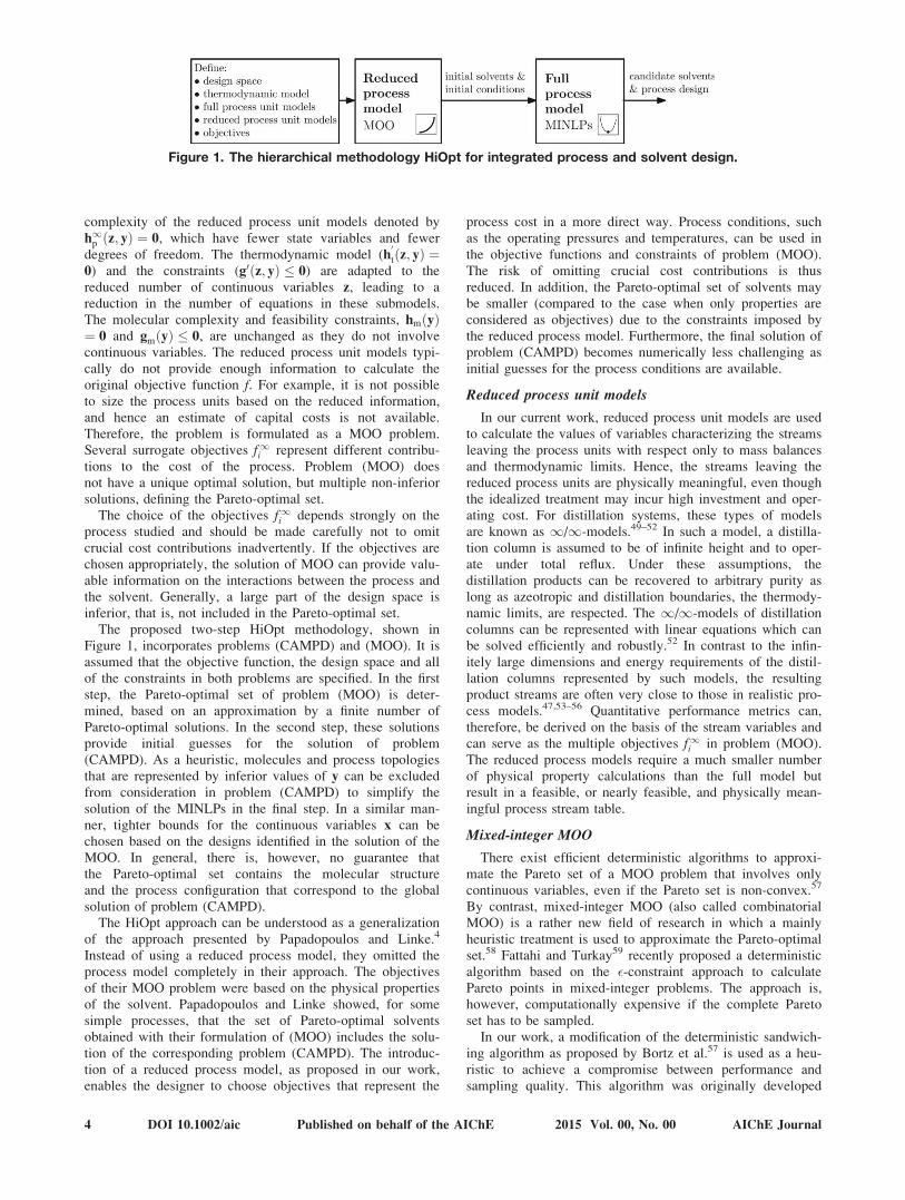
The proposed two-step HiOpt methodology, shown inFigure 1, incorporates problems (CAMPD) and (MOO). It isassumed that the objective function, the design space and allof the constraints in both problems are specified. In the firststep, the Pareto-optimal set of problem (MOO) is deter-mined, based on an approximation by a finite number ofPareto-optimal solutions. In the second step, these solutionsprovide initial guesses for the solution of problem(CAMPD). As a heuristic, molecules and process topologiesthat are represented by inferior values of y can be excludedfrom consideration in problem (CAMPD) to simplify thesolution of the MINLPs in the final step. In a similar man-ner, tighter bounds for the continuous variables x can bechosen based on the designs identified in the solution of theMOO. In general, there is, however, no guarantee thatthe Pareto-optimal set contains the molecular structureand the process configuration that correspond to the globalsolution of problem (CAMPD).

The HiOpt approach can be understood as a generalizationof the approach presented by Papadopoulos and Linke.4

Instead of using a reduced process model, they omitted theprocess model completely in their approach. The objectivesof their MOO problem were based on the physical propertiesof the solvent. Papadopoulos and Linke showed, for somesimple processes, that the set of Pareto-optimal solventsobtained with their formulation of (MOO) includes the solu-tion of the corresponding problem (CAMPD). The introduc-tion of a reduced process model, as proposed in our work,enables the designer to choose objectives that represent the

process cost in a more direct way. Process conditions, suchas the operating pressures and temperatures, can be used inthe objective functions and constraints of problem (MOO).The risk of omitting crucial cost contributions is thusreduced. In addition, the Pareto-optimal set of solvents maybe smaller (compared to the case when only properties areconsidered as objectives) due to the constraints imposed bythe reduced process model. Furthermore, the final solution ofproblem (CAMPD) becomes numerically less challenging asinitial guesses for the process conditions are available.

Reduced process unit models

In our current work, reduced process unit models are usedto calculate the values of variables characterizing the streamsleaving the process units with respect only to mass balancesand thermodynamic limits. Hence, the streams leaving thereduced process units are physically meaningful, even thoughthe idealized treatment may incur high investment and oper-ating cost. For distillation systems, these types of modelsare known as 1/1-models.49–52 In such a model, a distilla-tion column is assumed to be of infinite height and to oper-ate under total reflux. Under these assumptions, thedistillation products can be recovered to arbitrary purity aslong as azeotropic and distillation boundaries, the thermody-namic limits, are respected. The 1/1-models of distillationcolumns can be represented with linear equations which canbe solved efficiently and robustly.52 In contrast to the infin-itely large dimensions and energy requirements of the distil-lation columns represented by such models, the resultingproduct streams are often very close to those in realistic pro-cess models.47,53–56 Quantitative performance metrics can,therefore, be derived on the basis of the stream variables andcan serve as the multiple objectives f1i in problem (MOO).The reduced process models require a much smaller numberof physical property calculations than the full model butresult in a feasible, or nearly feasible, and physically mean-ingful process stream table.

Mixed-integer MOO

There exist efficient deterministic algorithms to approxi-mate the Pareto set of a MOO problem that involves onlycontinuous variables, even if the Pareto set is non-convex.57

By contrast, mixed-integer MOO (also called combinatorialMOO) is a rather new field of research in which a mainlyheuristic treatment is used to approximate the Pareto-optimalset.58 Fattahi and Turkay59 recently proposed a deterministicalgorithm based on the �-constraint approach to calculatePareto points in mixed-integer problems. The approach is,however, computationally expensive if the complete Paretoset has to be sampled.

In our work, a modification of the deterministic sandwich-ing algorithm as proposed by Bortz et al.57 is used as a heu-ristic to achieve a compromise between performance andsampling quality. This algorithm was originally developed

Figure 1. The hierarchical methodology HiOpt for integrated process and solvent design.


for continuous convex problems and is used to approximatethe Pareto-optimal set with only a small number of Paretopoints. Inner and outer approximations for the Pareto set areobtained iteratively, with increasing accuracy. The distancebetween the two approximations is used implicitly, via aratio of distances, to test for convergence within a user-defined tolerance dS (a scalar that is greater than 1, with 1corresponding to an exact match of the Pareto set). To calcu-late Pareto-optimal points, the algorithm makes use of theconcept of weighted-sum scalarization, that is, the multipleobjectives in problem (MOO) are replaced by their weightedsum f R, leading to a single-objective optimization problemthat yields one Pareto-optimal point

f Rðz; y; wÞ ¼XNf

i¼1

wi f1i ðz; yÞ (1)

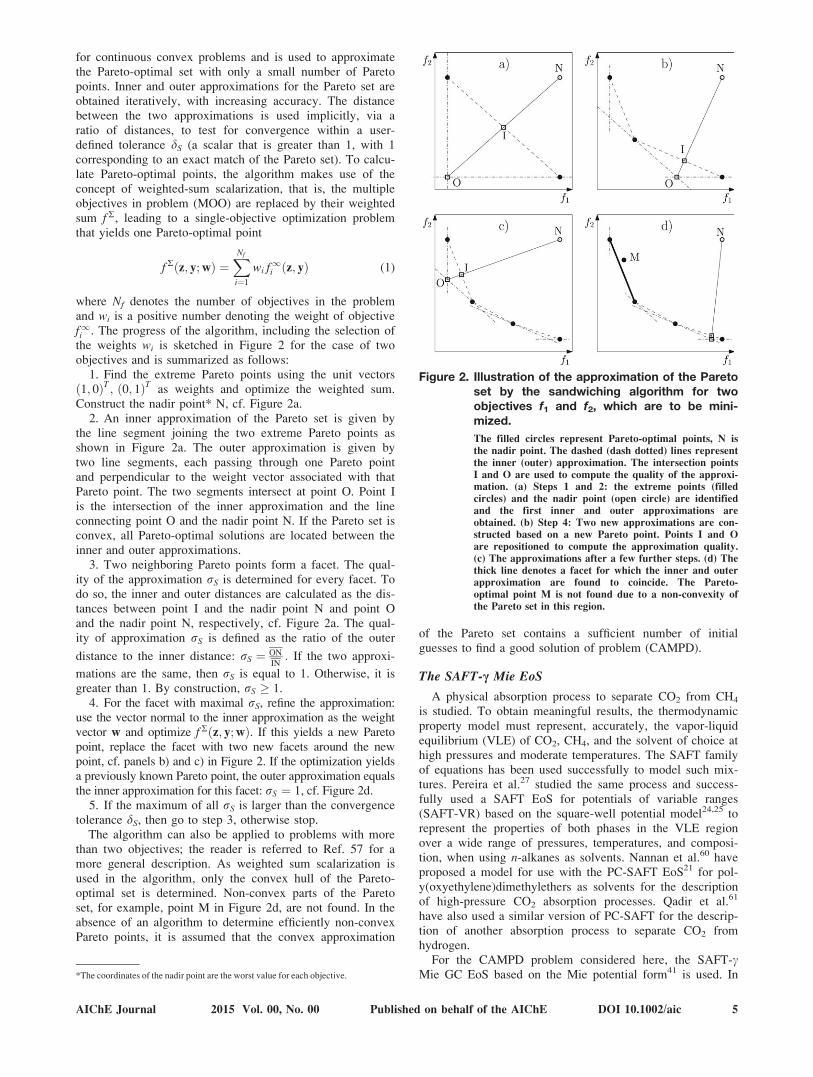
where Nf denotes the number of objectives in the problemand wi is a positive number denoting the weight of objectivef1i . The progress of the algorithm, including the selection ofthe weights wi is sketched in Figure 2 for the case of twoobjectives and is summarized as follows:

1. Find the extreme Pareto points using the unit vectorsð1; 0ÞT ; ð0; 1ÞT as weights and optimize the weighted sum.Construct the nadir point* N, cf. Figure 2a.

2. An inner approximation of the Pareto set is given bythe line segment joining the two extreme Pareto points asshown in Figure 2a. The outer approximation is given bytwo line segments, each passing through one Pareto pointand perpendicular to the weight vector associated with thatPareto point. The two segments intersect at point O. Point Iis the intersection of the inner approximation and the lineconnecting point O and the nadir point N. If the Pareto set isconvex, all Pareto-optimal solutions are located between theinner and outer approximations.

3. Two neighboring Pareto points form a facet. The qual-ity of the approximation rS is determined for every facet. Todo so, the inner and outer distances are calculated as the dis-tances between point I and the nadir point N and point Oand the nadir point N, respectively, cf. Figure 2a. The qual-ity of approximation rS is defined as the ratio of the outer

distance to the inner distance: rS ¼ ON

IN: If the two approxi-

mations are the same, then rS is equal to 1. Otherwise, it isgreater than 1. By construction, rS � 1.

4. For the facet with maximal rS, refine the approximation:use the vector normal to the inner approximation as the weightvector w and optimize f Rðz; y; wÞ. If this yields a new Paretopoint, replace the facet with two new facets around the newpoint, cf. panels b) and c) in Figure 2. If the optimization yieldsa previously known Pareto point, the outer approximation equalsthe inner approximation for this facet: rS ¼ 1, cf. Figure 2d.

5. If the maximum of all rS is larger than the convergencetolerance dS, then go to step 3, otherwise stop.

The algorithm can also be applied to problems with morethan two objectives; the reader is referred to Ref. 57 for amore general description. As weighted sum scalarization isused in the algorithm, only the convex hull of the Pareto-optimal set is determined. Non-convex parts of the Paretoset, for example, point M in Figure 2d, are not found. In theabsence of an algorithm to determine efficiently non-convexPareto points, it is assumed that the convex approximation

of the Pareto set contains a sufficient number of initialguesses to find a good solution of problem (CAMPD).

The SAFT-c Mie EoS

A physical absorption process to separate CO2 from CH4

is studied. To obtain meaningful results, the thermodynamicproperty model must represent, accurately, the vapor-liquidequilibrium (VLE) of CO2, CH4, and the solvent of choice athigh pressures and moderate temperatures. The SAFT familyof equations has been used successfully to model such mix-tures. Pereira et al.27 studied the same process and success-fully used a SAFT EoS for potentials of variable ranges(SAFT-VR) based on the square-well potential model24,25 torepresent the properties of both phases in the VLE regionover a wide range of pressures, temperatures, and composi-tion, when using n-alkanes as solvents. Nannan et al.60 haveproposed a model for use with the PC-SAFT EoS21 for pol-y(oxyethylene)dimethylethers as solvents for the descriptionof high-pressure CO2 absorption processes. Qadir et al.61

have also used a similar version of PC-SAFT for the descrip-tion of another absorption process to separate CO2 fromhydrogen.

For the CAMPD problem considered here, the SAFT-cMie GC EoS based on the Mie potential form41 is used. In

Figure 2. Illustration of the approximation of the Paretoset by the sandwiching algorithm for twoobjectives f1 and f2, which are to be mini-mized.

The filled circles represent Pareto-optimal points, N is

the nadir point. The dashed (dash dotted) lines represent

the inner (outer) approximation. The intersection points

I and O are used to compute the quality of the approxi-

mation. (a) Steps 1 and 2: the extreme points (filled

circles) and the nadir point (open circle) are identified

and the first inner and outer approximations are

obtained. (b) Step 4: Two new approximations are con-

structed based on a new Pareto point. Points I and O

are repositioned to compute the approximation quality.

(c) The approximations after a few further steps. (d) The

thick line denotes a facet for which the inner and outer

approximation are found to coincide. The Pareto-

optimal point M is not found due to a non-convexity of

the Pareto set in this region.

*The coordinates of the nadir point are the worst value for each objective.


contrast to the SAFT versions considered so far in studies ofsuch processes, SAFT-c Mie is a GC formulation and is thusideally suited for the representation of a large set of solventsin the process. It can be used to describe the properties ofthe pure component as well as the mixtures for both thevapor and liquid phases on an equal footing. For the VLE ofmixtures of CO2, CH4, and n-alkanes, it has been shown togive good agreement with experimental data.62 The exten-sion of the group parameter base to represent a large set ofsolvents is discussed later. Some basic characteristics of theSAFT-c Mie EoS are presented first for completeness.

In the SAFT-c Mie EoS, the molecules are described in

terms of interaction potential parameters of the segments

characterizing the various functional groups. Each molecule

is represented by Nk groups of type k and each group k con-

sists of one or more identical segments as defined by the

parameter m�k . Each segment is further characterized by a

shape factor, Sk; the shape factor characterizes the extent to

which the group’s segments contribute to the overall thermo-

dynamic properties of the molecule. The interactions

between two segments are modeled using the Mie (general-

ized Lennard–Jones) potential form. The Mie pair interaction

energy Ukl of two segments of types k and l is given as a

function of the distance r between the centers of the seg-

ments by41,63

UklðrÞ ¼ Ckl�klrkl

r

� �krkl

2rkl

r

� �kakl

� �(2)

where �kl is the depth of the potential well, rkl is the seg-ment diameter, kr

kl and kakl are the repulsive and attractive

exponents of the potential. The prefactor Ckl is given by

Ckl ¼kr

kl

krkl2ka

kl

krkl

kakl

� � kakl

krkl

2kakl

(3)

so that the minimum of the interaction energy is 2�kl.Six parameters, therefore, describe a (non-associating)

functional group k: the number of segments m�k , the potentialparameters rkk, ka

kk; krkk, and �kk, and the shape factor Sk.

This is augmented by unlike parameters to describe the inter-actions between two different types of segment k and l. Theunlike parameters can be calculated using the followingcombining rules41

rkl ¼ rkk1rll

2;

�kl ¼ ffiffiffiffiffiffiffiffiffiffi�kk�llp

;

kakl ¼ 31

ffiffiffiffiffiffiffiffiffiffiffiffiffiffiffiffiffiffiffiffiffiffiffiffiffiffiffiffiffiffiffiffika

kk23

kall23

q;

krkl ¼ 31

ffiffiffiffiffiffiffiffiffiffiffiffiffiffiffiffiffiffiffiffiffiffiffiffiffiffiffiffiffiffiffiffikr

kk23

krll23

q(4)

In some cases, the parameters �kl, kakl, and kr

kl are adjustedto best describe the target experimental data. In our work,the unlike dispersion energy parameter �kl is either obtainedfrom the relevant combining rule or estimated from experi-mental data, as described later. Other unlike interactions areobtained from the combining rules given in Eq. 4. In theSAFT-c Mie approach, it is also possible for the groups tohave association sites that mediate strong directional interac-tions such as hydrogen bonds,64,65 but this feature is notused in our current work. For further details of the SAFT-cMie EoS, the reader is referred to Ref. 41.

Description of the Case Study

CO2 absorption from natural gas

A prototypical process for the removal of CO2 from natu-ral gas is studied. Natural gas is usually produced at highpressure and often has a high concentration of CO2 (30 to50 mol %); in extreme cases, it may have a CO2 concentra-tion of 70 mol %.27 The CO2 may be of natural origin ormay stem from the injection of CO2 into near-depleted reser-voirs as part of enhanced oil recovery.27 In order to intro-duce natural gas into the distribution system, for example,pipelines, the fraction of CO2 must be reduced to below3 mol %.66 As the CO2 concentration in the natural gas feedcan be appreciable, removing it by chemical absorption withheat regeneration of the solvent is expensive. Physicalabsorption processes in which CO2 is stripped from theloaded non-reactive solvent merely by reducing the pressure,without the application of heat, becomes a favorableoption.67 In such a process, the solvent should exhibit a highcapacity for CO2, a high selectivity of CO2 compared to nat-ural gas and a low vapor pressure (to minimize solventlosses). Achieving these targets depends not only on the sol-vent’s molecular structure but also on the process conditions.The optimal solvent can, therefore, only be identified withconfidence by considering the integrated solvent and processdesign problem.

In our current work, we adopt the problem statement, theprocess flow sheet, and the process unit models of Ref. 27.The process flow sheet is given in Figure 3. The natural gasfeed, Stream (1), is considered to be a binary mixture ofCH4 and CO2 at high pressure. It is expanded and fed to acounter-current absorption column. The solvent absorbs CO2

preferentially and a cleaned gaseous stream leaves the col-umn at the top of the absorber as Stream (3). The pressureof the CO2-rich solvent leaving the bottom of the absorber,Stream (4), is then reduced to regenerate the solvent. Theresulting CO2-rich vapor phase is separated from the liquidsolvent in a flash drum and purged from the process viaStream (6). After regeneration, the lean solvent is pumpedback to the absorber. To compensate for solvent losses in thegaseous product streams, a small feed, Stream (8), of freshsolvent is also supplied.

The specifications of the process are mainly adopted fromRef. 27; the full process model divided into fixed variables

Figure 3. Flow sheet for the process considered toseparate CO2 from a mixture with CH4 byhigh-pressure physical absorption.27


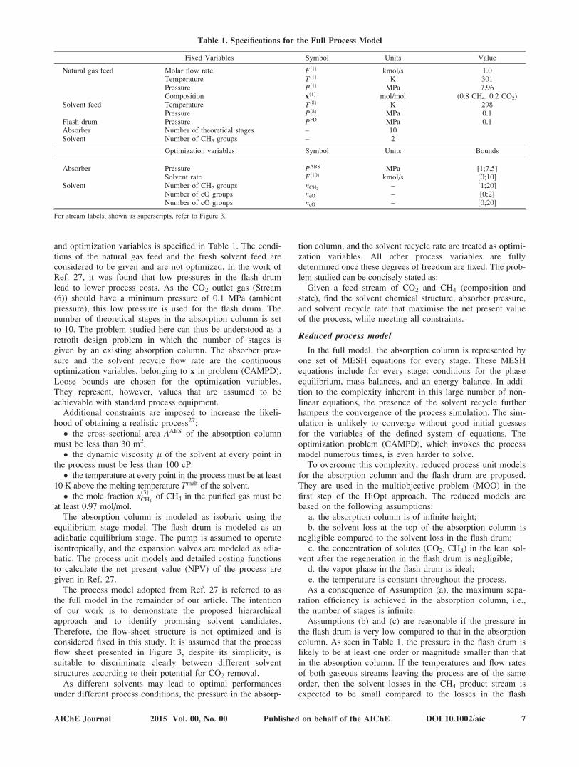
and optimization variables is specified in Table 1. The condi-tions of the natural gas feed and the fresh solvent feed areconsidered to be given and are not optimized. In the work ofRef. 27, it was found that low pressures in the flash drumlead to lower process costs. As the CO2 outlet gas (Stream(6)) should have a minimum pressure of 0.1 MPa (ambientpressure), this low pressure is used for the flash drum. Thenumber of theoretical stages in the absorption column is setto 10. The problem studied here can thus be understood as aretrofit design problem in which the number of stages isgiven by an existing absorption column. The absorber pres-sure and the solvent recycle flow rate are the continuousoptimization variables, belonging to x in problem (CAMPD).Loose bounds are chosen for the optimization variables.They represent, however, values that are assumed to beachievable with standard process equipment.

Additional constraints are imposed to increase the likeli-hood of obtaining a realistic process27:� the cross-sectional area AABS of the absorption column

must be less than 30 m2.� the dynamic viscosity l of the solvent at every point in

the process must be less than 100 cP.� the temperature at every point in the process must be at least

10 K above the melting temperature Tmelt of the solvent.� the mole fraction x

ð3ÞCH4

of CH4 in the purified gas must beat least 0.97 mol/mol.

The absorption column is modeled as isobaric using theequilibrium stage model. The flash drum is modeled as anadiabatic equilibrium stage. The pump is assumed to operateisentropically, and the expansion valves are modeled as adia-batic. The process unit models and detailed costing functionsto calculate the net present value (NPV) of the process aregiven in Ref. 27.

The process model adopted from Ref. 27 is referred to asthe full model in the remainder of our article. The intentionof our work is to demonstrate the proposed hierarchicalapproach and to identify promising solvent candidates.Therefore, the flow-sheet structure is not optimized and isconsidered fixed in this study. It is assumed that the processflow sheet presented in Figure 3, despite its simplicity, issuitable to discriminate clearly between different solventstructures according to their potential for CO2 removal.

As different solvents may lead to optimal performancesunder different process conditions, the pressure in the absorp-

tion column, and the solvent recycle rate are treated as optimi-zation variables. All other process variables are fullydetermined once these degrees of freedom are fixed. The prob-lem studied can be concisely stated as:

Given a feed stream of CO2 and CH4 (composition andstate), find the solvent chemical structure, absorber pressure,and solvent recycle rate that maximise the net present valueof the process, while meeting all constraints.

Reduced process model

In the full model, the absorption column is represented byone set of MESH equations for every stage. These MESHequations include for every stage: conditions for the phaseequilibrium, mass balances, and an energy balance. In addi-tion to the complexity inherent in this large number of non-linear equations, the presence of the solvent recycle furtherhampers the convergence of the process simulation. The sim-ulation is unlikely to converge without good initial guessesfor the variables of the defined system of equations. Theoptimization problem (CAMPD), which invokes the processmodel numerous times, is even harder to solve.

To overcome this complexity, reduced process unit modelsfor the absorption column and the flash drum are proposed.They are used in the multiobjective problem (MOO) in thefirst step of the HiOpt approach. The reduced models arebased on the following assumptions:

a. the absorption column is of infinite height;b. the solvent loss at the top of the absorption column is

negligible compared to the solvent loss in the flash drum;c. the concentration of solutes (CO2, CH4) in the lean sol-

vent after the regeneration in the flash drum is negligible;d. the vapor phase in the flash drum is ideal;e. the temperature is constant throughout the process.As a consequence of Assumption (a), the maximum sepa-

ration efficiency is achieved in the absorption column, i.e.,the number of stages is infinite.

Assumptions (b) and (c) are reasonable if the pressure inthe flash drum is very low compared to that in the absorptioncolumn. As seen in Table 1, the pressure in the flash drum islikely to be at least one order or magnitude smaller than thatin the absorption column. If the temperatures and flow ratesof both gaseous streams leaving the process are of the sameorder, then the solvent losses in the CH4 product stream isexpected to be small compared to the losses in the flash

Table 1. Specifications for the Full Process Model

Fixed Variables Symbol Units Value

Natural gas feed Molar flow rate Fð1Þ kmol/s 1.0Temperature Tð1Þ K 301Pressure Pð1Þ MPa 7.96Composition xð1Þ mol/mol (0.8 CH4, 0.2 CO2)

Solvent feed Temperature Tð8Þ K 298Pressure Pð8Þ MPa 0.1

Flash drum Pressure PFD MPa 0.1Absorber Number of theoretical stages – 10Solvent Number of CH3 groups – 2

Optimization variables Symbol Units Bounds

Absorber Pressure PABS MPa [1;7.5]Solvent rate Fð10Þ kmol/s [0;10]

Solvent Number of CH2 groups nCH2– [1;20]

Number of eO groups neO – [0;2]Number of cO groups ncO – [0;20]

For stream labels, shown as superscripts, refer to Figure 3.


drum. Furthermore, the gas solubility in the flash drum isdrastically reduced by the large pressure drop, leading to avery small concentration of solutes in the solvent leaving theflash drum.

Assumption (d) is reasonable for low pressures. The pres-sure in the flash drum of 0.1 MPa is considered to be suffi-ciently low.

Assumption (e) is introduced in order to eliminate energybalances and other caloric calculations from the process inthis step. In simulations with the full model, it is observedthat the temperature is roughly constant throughout the pro-cess. This can be explained by the lack of significant heatinput/output in the process, without units such as evaporatorsor condensers, in the process. The impact of the absorptionenthalpy on the energy balances is partly compensated bypressure changes. For instance, the pressure drop betweenthe absorber and the flash drum leads to a release of energythat is partly used to desorb the gas in the flash drum. Thisapproximation is thus reasonable.

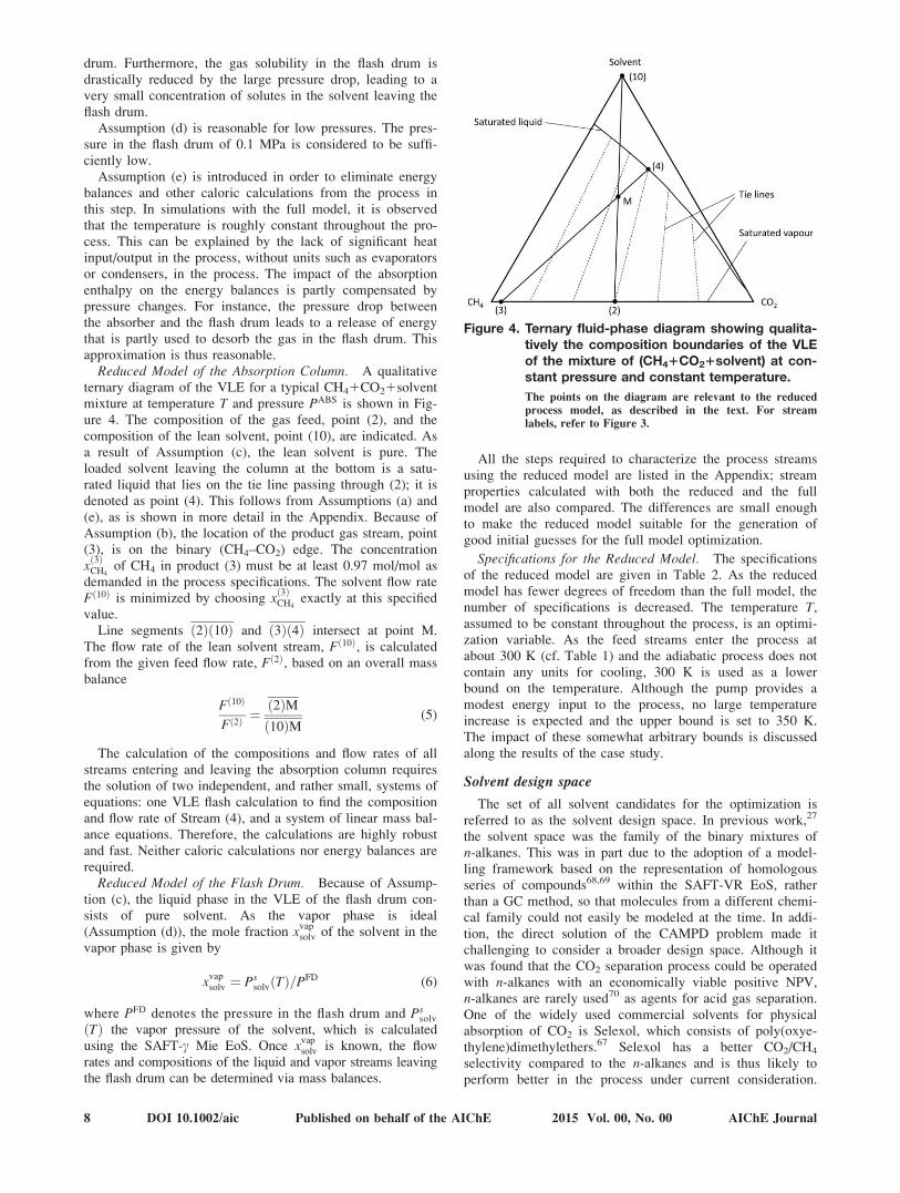
Reduced Model of the Absorption Column. A qualitativeternary diagram of the VLE for a typical CH41CO21solventmixture at temperature T and pressure PABS is shown in Fig-ure 4. The composition of the gas feed, point (2), and thecomposition of the lean solvent, point (10), are indicated. Asa result of Assumption (c), the lean solvent is pure. Theloaded solvent leaving the column at the bottom is a satu-rated liquid that lies on the tie line passing through (2); it isdenoted as point (4). This follows from Assumptions (a) and(e), as is shown in more detail in the Appendix. Because ofAssumption (b), the location of the product gas stream, point(3), is on the binary (CH4–CO2) edge. The concentrationxð3ÞCH4

of CH4 in product (3) must be at least 0.97 mol/mol asdemanded in the process specifications. The solvent flow rateFð10Þ is minimized by choosing x

ð3ÞCH4

exactly at this specifiedvalue.

Line segments ð2Þð10Þ and ð3Þð4Þ intersect at point M.The flow rate of the lean solvent stream, Fð10Þ, is calculatedfrom the given feed flow rate, Fð2Þ, based on an overall massbalance

Fð10Þ

Fð2Þ¼ ð2ÞMð10ÞM

(5)

The calculation of the compositions and flow rates of allstreams entering and leaving the absorption column requiresthe solution of two independent, and rather small, systems ofequations: one VLE flash calculation to find the compositionand flow rate of Stream (4), and a system of linear mass bal-ance equations. Therefore, the calculations are highly robustand fast. Neither caloric calculations nor energy balances arerequired.

Reduced Model of the Flash Drum. Because of Assump-tion (c), the liquid phase in the VLE of the flash drum con-sists of pure solvent. As the vapor phase is ideal(Assumption (d)), the mole fraction xvap

solv of the solvent in thevapor phase is given by

xvapsolv ¼ Ps

solvðTÞ=PFD (6)

where PFD denotes the pressure in the flash drum and Pssolv

ðTÞ the vapor pressure of the solvent, which is calculatedusing the SAFT-c Mie EoS. Once xvap

solv is known, the flowrates and compositions of the liquid and vapor streams leavingthe flash drum can be determined via mass balances.

All the steps required to characterize the process streamsusing the reduced model are listed in the Appendix; streamproperties calculated with both the reduced and the fullmodel are also compared. The differences are small enoughto make the reduced model suitable for the generation ofgood initial guesses for the full model optimization.

Specifications for the Reduced Model. The specificationsof the reduced model are given in Table 2. As the reducedmodel has fewer degrees of freedom than the full model, thenumber of specifications is decreased. The temperature T,assumed to be constant throughout the process, is an optimi-zation variable. As the feed streams enter the process atabout 300 K (cf. Table 1) and the adiabatic process does notcontain any units for cooling, 300 K is used as a lowerbound on the temperature. Although the pump provides amodest energy input to the process, no large temperatureincrease is expected and the upper bound is set to 350 K.The impact of these somewhat arbitrary bounds is discussedalong the results of the case study.

Solvent design space

The set of all solvent candidates for the optimization isreferred to as the solvent design space. In previous work,27

the solvent space was the family of the binary mixtures ofn-alkanes. This was in part due to the adoption of a model-ling framework based on the representation of homologousseries of compounds68,69 within the SAFT-VR EoS, ratherthan a GC method, so that molecules from a different chemi-cal family could not easily be modeled at the time. In addi-tion, the direct solution of the CAMPD problem made itchallenging to consider a broader design space. Although itwas found that the CO2 separation process could be operatedwith n-alkanes with an economically viable positive NPV,n-alkanes are rarely used70 as agents for acid gas separation.One of the widely used commercial solvents for physicalabsorption of CO2 is Selexol, which consists of poly(oxye-thylene)dimethylethers.67 Selexol has a better CO2/CH4

selectivity compared to the n-alkanes and is thus likely toperform better in the process under current consideration.

Figure 4. Ternary fluid-phase diagram showing qualita-tively the composition boundaries of the VLEof the mixture of (CH41CO21solvent) at con-stant pressure and constant temperature.

The points on the diagram are relevant to the reduced

process model, as described in the text. For stream

labels, refer to Figure 3.


Driven by this motivation, the solvent space is extended tolinear alkyl ethers. Molecules containing up to 22 alkylgroups and 21 ether groups are considered to ensure that allliquid linear alkanes and ethers are included. This is a broadset of structures within the families considered: it containsmore than 200 candidate molecules with vapor pressures andmelting points that make them suitable for use as a solventin the process.

Although the solvent design space is limited to ether struc-tures, it contains some interesting chemicals whose perform-ance and suitability can be directly compared in the study:� the family of n-alkanes (CH3[CH2]nCH3),� the family of poly(oxyethylene)dimethylethers (CH3O

[CH2CH2O]nCH3) contained in the Selexol solvent,� the family of poly(oxymethylene)dimethylethers

(CH3O[CH2O]nCH3), also known as OMEs, which have thehighest oxygen content of all linear alkyl ethers and whichare novel, natural gas-based fuel additives, which could beavailable at low cost in the future.71

SAFT-c Mie GC Models for Relevant Mixtures

Group definition

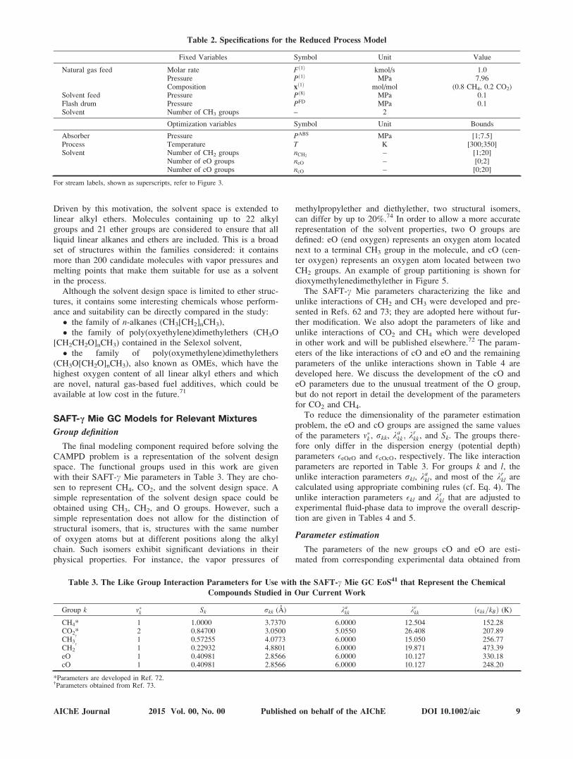
The final modeling component required before solving theCAMPD problem is a representation of the solvent designspace. The functional groups used in this work are givenwith their SAFT-c Mie parameters in Table 3. They are cho-sen to represent CH4, CO2, and the solvent design space. Asimple representation of the solvent design space could beobtained using CH3, CH2, and O groups. However, such asimple representation does not allow for the distinction ofstructural isomers, that is, structures with the same numberof oxygen atoms but at different positions along the alkylchain. Such isomers exhibit significant deviations in theirphysical properties. For instance, the vapor pressures of

methylpropylether and diethylether, two structural isomers,can differ by up to 20%.74 In order to allow a more accuraterepresentation of the solvent properties, two O groups aredefined: eO (end oxygen) represents an oxygen atom locatednext to a terminal CH3 group in the molecule, and cO (cen-ter oxygen) represents an oxygen atom located between twoCH2 groups. An example of group partitioning is shown fordioxymethylenedimethylether in Figure 5.

The SAFT-c Mie parameters characterizing the like andunlike interactions of CH2 and CH3 were developed and pre-sented in Refs. 62 and 73; they are adopted here without fur-ther modification. We also adopt the parameters of like andunlike interactions of CO2 and CH4 which were developedin other work and will be published elsewhere.72 The param-eters of the like interactions of cO and eO and the remainingparameters of the unlike interactions shown in Table 4 aredeveloped here. We discuss the development of the cO andeO parameters due to the unusual treatment of the O group,but do not report in detail the development of the parametersfor CO2 and CH4.

To reduce the dimensionality of the parameter estimationproblem, the eO and cO groups are assigned the same valuesof the parameters m�k , rkk, ka

kk; krkk, and Sk. The groups there-

fore only differ in the dispersion energy (potential depth)parameters �eOeO and �cOcO, respectively. The like interactionparameters are reported in Table 3. For groups k and l, theunlike interaction parameters rkl, ka

kl, and most of the krkl are

calculated using appropriate combining rules (cf. Eq. 4). Theunlike interaction parameters �kl and kr

kl that are adjusted toexperimental fluid-phase data to improve the overall descrip-tion are given in Tables 4 and 5.

Parameter estimation

The parameters of the new groups cO and eO are esti-mated from corresponding experimental data obtained from

Table 2. Specifications for the Reduced Process Model

Fixed Variables Symbol Unit Value

Natural gas feed Molar rate Fð1Þ kmol/s 1.0Pressure Pð1Þ MPa 7.96Composition xð1Þ mol/mol (0.8 CH4, 0.2 CO2)

Solvent feed Pressure Pð8Þ MPa 0.1Flash drum Pressure PFD MPa 0.1Solvent Number of CH3 groups – 2

Optimization variables Symbol Unit Bounds

Absorber Pressure PABS MPa [1;7.5]Process Temperature T K [300;350]Solvent Number of CH2 groups nCH2

– [1;20]Number of eO groups neO – [0;2]Number of cO groups ncO – [0;20]

For stream labels, shown as superscripts, refer to Figure 3.

Table 3. The Like Group Interaction Parameters for Use with the SAFT-c Mie GC EoS41 that Represent the Chemical

Compounds Studied in Our Current Work

Group k m�k Sk rkk (A) kakk kr

kk ð�kk=kBÞ (K)

CH4* 1 1.0000 3.7370 6.0000 12.504 152.28CO2* 2 0.84700 3.0500 5.0550 26.408 207.89CH3

†

1 0.57255 4.0773 6.0000 15.050 256.77CH2

†

1 0.22932 4.8801 6.0000 19.871 473.39eO 1 0.40981 2.8566 6.0000 10.127 330.18cO 1 0.40981 2.8566 6.0000 10.127 248.20

*Parameters are developed in Ref. 72.†Parameters obtained from Ref. 73.


the DETHERM database.75 Details of the implementation,variance models, and error function are given in the Appendix.

Estimation from Pure Component Data. In a first step, thevapor pressures and liquid densities (in either saturated or com-pressed states) of pure ethers are considered to obtain the likeparameters for the eO and cO groups and their unlike interac-tions parameters with each other and with the CH2 and CH3

groups. The compounds used in the estimation and the tempera-ture ranges of the experimental data are specified in Table 6.The original data sources can be found in Refs. 47, 74, 76–89.The following seven parameters are estimated simultaneouslyfrom the data: SeO; reO;eO; kr

eO;eO; �eO;eO; �cO;cO; �eO;CH3, and

�eO;CH2. The remaining eO and cO group parameters are either

fixed to constant values or coupled during the estimationaccording to the following constraints

m�cO ¼ m�eO ¼ 1 (7)

kacO;cO ¼ ka

eO;eO ¼ 6 (8)

ScO ¼ SeO (9)

rcO;cO ¼ reO;eO (10)

krcO;cO ¼ kr

eO;eO (11)

�cO;CH3

�CRcO;CH3

¼ �eO;CH3

�CReO;CH3

(12)

�cO;CH2

�CRcO;CH2

¼ �eO;CH2

�CReO;CH2

(13)

�cO;eO ¼ �CRcO;eO (14)

where the superscript CR denotes the value obtained by apply-ing the relevant combining rule, cf. Eq. 4. Equations 12 and 13are equivalent to imposing the same deviation fromcombining-rule behavior (which is often represented by thebinary interaction parameter kij for a geometric-mean rule) forthe interaction energy of the eO and cO groups with the alkylgroups. The percentage absolute average deviation (%AAD)

from the experimental data obtained with the optimal set ofparameters is given in Table 6. The calculated vapor pressuresand liquid densities are compared to experimental values inFigures 6–11. The calculated vapor pressures are found to bein good agreement with the data for the majority of the etherstructures despite the small number of parameters, cf. Figures6–8. Although the %AAD is larger than 10% in some cases,the model clearly provides good qualitative agreement withthe data, which is crucial for solvent design. Structural iso-mers, such as methylpropylether and diethylether, are rankedcorrectly, cf. Figure 6. The deviations for the liquid densityare generally below 1%, cf. Table 6 and Figures 9–11.

Parameter Estimation from Gas Solubility Data. In asecond step, high-pressure vapor-liquid equilibria and solu-bility data of CO2 and CH4 in the ether solvents are consid-ered: the unlike interaction parameter �eO;CO2

is estimatedfrom experimental solubility data of CO2 in poly(oxyethyle-ne)dimethylethers,91,92 and the unlike interaction parameter�eO;CH4

is fitted to high-pressure VLE data of CH4 and meth-ylal (CH3OCH2OCH3).93 The following parameters werecoupled during the estimation to provide values for theunlike interaction parameters �cO;CO2

and �cO;CH4

�cO;CO2

�CRcO;CO2

¼ �eO;CO2

�CReO;CO2

�cO;CH4

�CRcO;CH4

¼ �eO;CH4

�CReO;CH4

(15)

Comparisons of the calculations with the SAFT-c MieEoS and the experimental data91–93 used in the estimationare given in Figures 12–14. A good description of the solu-bility of CO2 is obtained with the SAFT-c Mie approach forthe available datasets, cf. Figures 12 and 13. It can be seenin Figure 14 that the calculated VLE for the CH41methylalmixture exhibits some deviations from the experimental val-ues in the higher-pressure critical region of the mixtures.The pressure of the process in this study, however, neverexceeds 10 MPa. The unlike repulsive exponent parameterkr

eO;CH4was calculated to comply with the combining rule

given in Eq. 4 during the estimation. The alternative of add-ing this parameter to the set of estimated parameters doesnot improve the quality of the description of the VLE signifi-cantly. Despite the general deviations in the VLE, the solu-bility of CH4 in methylal is represented well (left part ofFigure 14). The set of experimental solubility data of themixtures of CO2 and CH4 with alkyl ethers is limited; addi-tional measurements, particularly with longer ethers, wouldallow for a more detailed assessment of the proposed model.

Because of the deviations observed for the vapor pressureand the paucity of validation data for solubility, the proposedmodel is not suitable for the full detailed design of processequipment. Nevertheless, it is accurate enough to reflect theeffects of the solvent chemical structure on the process

Figure 5. Group partitioning for dioxymethylenedime-thylether for implementation in the SAFT-cMie EoS41: 2 CH3, 2 CH2, 2 eO, 1 cO.

Table 4. Values of the Unlike Dispersion Energy Parameter

(�kl=kBÞ in K that Represent the Chemical Compounds Studied

in Our Current Work, for Use with the SAFT-c Mie GC EoS41

k/l CO2 CH3 CH2 eO cO

CH4 144.72* 193.97 243.13 210.13 182.18CO2 187.98 275.15 327.31 283.78CH3 350.77

†

301.77 261.63CH2 408.05 353.78eO 286.27

*Parameters are developed in Ref. 72.†Parameters obtained from Ref. 73.

Table 5. Values of the Repulsive Exponent krkl of the Unlike

Interaction Potential that Represent the Chemical

Compounds Studied in Our Current Work, for Use with the

SAFT-c Mie GC EoS41

k/l CO2 CH3 CH2

CH4 11.950 12.628 12.642CO2 15.581 21.982

Combinations not given in this table are calculated by the combining rule Eq. 4.


performance and trends in processing conditions. Due to thestrong physical basis of the SAFT-c Mie approach and thecomparably small number of parameters, the predictive capa-bilities of the thermodynamic model are expected to be well-suited to identify novel solvent candidates. Once the optimalsolvent candidate has been identified, the thermodynamicmodel should be adjusted if a more detailed process designis desired.

Representation of the solvent design space

Having identified the functional groups that are used tocharacterize the solvent molecules, we can now define thevector y of integer variables that represent how many timeseach functional group occurs in the solvent molecule. We

first note that the number of CH3 end groups, nCH3is fixed

and equal to 2 for all molecules in the solvent design spaceas only linear molecules are considered. The integer decisionvariables are

nCH2; neO; ncO½ � (16)

where nk denotes the number of groups of type k. Thebounds on these variables are listed in Table 1. The solventmolecule comprises a minimum of one CH2 group based onthe physical argument that a molecule smaller than propanewould be too volatile and would not be suitable as a solvent.A maximum of two eO groups is allowed in the molecules,since there are only two CH3 groups.

Given that only linear molecules are considered in this casestudy, only one molecule feasibility constraint (gmðyÞ � 0)

Table 6. Percentage Average Absolute Deviations %AAD of Vapor Pressures and Liquid Densities of the Calculations Using

the SAFT-c Mie EoS with the Group Parameters given in Tables 3–5 from the Corresponding Experimental Data

Vapor Pressure Liquid Density

Compound T (K) n %AAD T (K) n %AAD

CH3OCH2CH3 273–393 13 4.3 273–392 4 0.3CH3O(CH2)2CH3 254–333 22 9.5 273–308 5 0.7CH3O(CH2)3CH3 256–343 10 13.4 273–315 7 1.1CH3CH2OCH2CH3 250–421 17 12.0 273–423 16 0.3CH3(CH2)2O(CH2)2CH3 293–388 11 14.3 288–333 6 1.6CH3(CH2)3O(CH2)3CH3 356–404 11 17.7 273–323 5 1.8CH3O(CH2CH2O)CH3 358–533 14 4.1 198–273 10 0.3CH3O(CH2CH2O)2CH3 330–434 11 24.6 283–383 6 0.7CH3O(CH2CH2O)3CH3 361–490 8 4.4 283–423 8 0.6CH3O(CH2CH2O)4CH3 373–533 17 9.1 283–423 15 0.5CH3O(CH2CH2O)5CH3 0 283–423 15 0.5CH3O(CH2O)CH3 185 2315 9 11.7 233–363 14 0.6CH3O(CH2O)2CH3 297–375 6 6.9 293–363 8 0.5CH3O(CH2O)3CH3 314–426 8 6.1 293–363 8 0.4CH3O(CH2O)4CH3 348–472 8 2.9 293–363 8 0.3CH3O(CH2O)5CH3 364–511 9 3.3 0

n is the number of data points and T is the temperature range. %AAD 5 100=n �Xn

i¼1jðumod

i 2uexpi Þ=u

expi j, where umod denotes the calculated property value and

uexp the measured value.

Figure 6. Logarithmic representation of the saturatedvapor pressure Ps with respect to tempera-ture T.

The curves represent the calculations of the SAFT-cMie EoS41 with the group parameters specified in

Tables 3–5 and the symbols denote the corresponding

experimental data74,76–79: methylethylether (�), diethy-

lether (�), methylpropylether (�), methylbutylether (w),

dipropylether (�), and dibutylether (W). The experimen-

tal critical points90 are indicated by *.




experimental data80–82: dimethoxyethane (�), di(oxye-

thylene)dimethyl ether (�), tri(oxyethylene)dimethy-

lether (W), and tetra(oxyethylene)dimethylether (�). The

experimental critical points90 are indicated by *.


needs to be imposed. We ensure that each cO group is associ-ated with two CH2 groups as follows

ncO2nCH211 � 0 (17)

Hierarchical Solvent and Process Design for CO2

Absorption

Optimization with the reduced model

Problem Formulation. As the first step of the HiOptapproach, problem (MOO) is formulated and solved. The

equations of the reduced model described above serve as thereduced process unit model (h1p ðz; yÞ ¼ 0Þ. The vector z ofcontinuous variables is given by

z ¼ T;PABS� �T

(18)

where T is the temperature of the isothermal reduced processmodel in K, and PABS is the absorber pressure in MPa. Thevector of integer variables is the same as for the full model,cf. Eq. 16. The bounds on z and y are given in Table 2.

The reduced model provides neither internal flow rates inthe absorption column nor energetic variables such as the




experimental data78,83: methylal (�), di(oxymethylene)-

dimethylether (�), tri(oxymethylene)dimethylether (�),

tetra(oxymethylene)dimethylether (W), and penta(oxyme-

thylene)dimethylether (�). The experimental critical

points90 are indicated by *.

Figure 9. Dependence of the molar liquid density qliq

with respect to temperature T.



experimental data78,84–86: methylethylether (�, satu-

rated-liquid), diethylether (�, saturated-liquid), methyl-

propylether (�, compressed-liquid at 1.013 bar),

methylbutylether (w, compressed-liquid at 1.013 bar),

dipropylether (�, compressed-liquid at 1.013 bar), and

dibutylether (W, compressed-liquid at 1.013 bar).

Figure 10. Dependence of the molar compressed-liquiddensity qliq with respect to temperature T.

The curves represent the calculations of the SAFT-c Mie

EoS41 with the group parameters specified in Tables 3–5

and the symbols denote the corresponding experimental

data87,88: dimethoxyethane (�, at 1.013 bar), di(oxyethyle-

ne)dimethylether (�, at 10 bar), tri(oxyethylene)dimethy-

lether (W, at 10 bar), tetra(oxyethylene)dimethylether

(�, at 10 bar), and penta(oxyethylene)dimethylether (�,

at 10 bar).

Figure 11. Dependence of the molar liquid density qliq

with respect to temperature T.



experimental data47,89: methylal (�, saturated-liquid),

di(oxymethylene)dimethylether (�, compressed-liquid at

1.013 bar), tri(oxymethylene)dimethylether (�, at 1.013

bar), tetra(oxymethylene)dimethylether (W, compressed-

liquid at 1.013 bar), and penta(oxymethylene)dimethy-

lether (�, compressed-liquid at 1.013 bar).


power consumption of the pump. The NPV, which is relatedto the sales of purified gas minus the capital and operatingcosts for the separation,27 cannot be calculated due to thislack of information and the NPV cannot, therefore, be used asan objective in the optimization. To address this issue, threeobjective functions that represent different contributions to theNPV are used at this stage of the hierarchical optimization.The gas sales are directly proportional to the molar flow rateof Stream (3) (the “product flow rate”), which is, therefore,chosen as the first objective, to be maximized

maxz;y

f11 ðz; yÞ ¼ Fð3Þ (19)

All molar flow rates FðiÞ are specified in kmol/s. Toaccount for the sizes of the process units, and thus, to penal-ize the capital cost of the absorber, pump, and flash drum,the recycle mass flow rate of solvent in kg/s (the “solventflow rate”) is used as a second objective to be minimized

minz;y

f12 ðz; yÞ ¼ Fð10Þ �MWsolv (20)

where the molecular mass of the solvent in kg/kmol isdenoted by MWsolv. A final contribution to the overall pro-cess cost is the solvent loss. It is equal to the mass flow rateof solvent that must be supplied to the process and is penal-ized by minimizing a third objective

minz;y

f13 ðz; yÞ ¼ Fð8Þ �MWsolv (21)

The price of the solvent is not accounted for in this work.It is assumed that the differences in the production costs ofthe solvents are negligible. It is difficult to estimate produc-tion costs for chemicals without large errors, especially forcomponents which are not being produced at present.The results, however, give an indication of the molecularstructure of the optimal solvent and can be seen as a recom-mendation for further studies focused on the development ofnew cost efficient production processes for the optimalsolvents.

The constraints g0ðz; yÞ � 0 are defined according to thedescription of the case study

lðTÞ2100 � 0 (22)

0:972xð3ÞCH4� 0 (23)

where l is the solvent’s viscosity (in cP) and xð3ÞCH4

is themole fraction of methane in Stream (3). The viscosity is esti-mated by the method of Sastri and Rao.94 Further, there is aconstraint on the normal melting point Tmelt of the solvent(in K) for which two cases are considered:

Figure 12. Pressure-mole fraction (liquid-phase) iso-thermal slices of the vapor-liquid-phaseequilibrium envelope for the binary mixtures ofCO2 and di(oxyethylene)dimethylether (—; �),tri(oxyethylene)dimethylether (– –; �),and tetra(oxyethylene)dimethylether (� � �; w),at T 5 313.15 K.



experimental data.91

Figure 13. Pressure-mole fraction (liquid-phase) iso-thermal slices of the vapor-liquid-phaseequilibrium envelope for the binary mixtureof CO2 and di(oxyethylene)dimethylether atdifferent temperatures: T 5 298.15 K (—; �),T 5 313.15 K – –; �), T 5 333.15 K � � �; w).




Figure 14. Pressure-mole fraction isothermal slices ofthe VLE envelope in the binary mixture ofmethane and methylal at different tempera-tures: T 5 274 K (�), T 5 313 K (�), T 5 253 K(w), T 5 394 K (�), T 5 432 K (�).





Case 1 : Tmelt2T110 � 0 (24)

Case 2 : Tmelt2T130 � 0 (25)

In the base Case 1, the process temperature is requested tobe at least 10 K above the melting temperature of the sol-vent. It was found that this constraint is active during theoptimizations. Thus, the accuracy of the estimated meltingpoints is crucial for the validity of the results. In our currentwork, the GC method of Marrero and Gani95 is used. In theAppendix, we show that the melting point is underestimatedfor some compounds in the solvent space. An additionalsafety margin of 20 K is added in Case 2 to reduce the riskof obtaining a process in which the solvent solidifies. Onecould also adopt the chance-constrained approach of Mara-nas96 to treat the effect of this uncertainty more formally.

Computation of the Pareto Set. The reduced processmodel is implemented in gPROMS.97 The SAFT-c Mie prop-erty model is implemented in Fortran62 and accessed via agPROMS Foreign Object. gPROMS provides an outer approx-imation/equality relaxation/augmented penalty (OAERAP)solver for MINLP problems,98,99 which is used to solve alloptimization problems in our work. The sandwiching algo-rithm for the MOOs is implemented in MATLAB.100 Theconvergence tolerance for sandwiching is chosen to bedS ¼ 1:03. The algorithm identifies 10 Pareto-optimal pointsto approximate the Pareto set.

Results and Discussion. For Case 1 with melting pointConstraint (24), the values of the three objectives for the 10Pareto-optimal points are depicted in Figure 15. The productflow rate and the solvent flow rate are shown on the horizon-tal and vertical axes, respectively. Different ranges of valuesof the solvent loss are represented by the different symbols.Solutions that lie near the lower right-hand corner of thegraph are desirable from the point of view of objectives f11and f12 . The solvents corresponding to the Pareto-optimalpoints are listed in Table 7 using an identifier (ID); the IDsare also shown in Figure 15. The values of the continuousoptimization variables in z at the Pareto-optima are alsolisted in Table 7.

Among the 10 Pareto-optimal points, there are six differ-ent solvent structures. These principally correspond to poly(oxymethylene)dimethylethers (IDs 1–5), the chemical fam-

ily with the largest oxygen content among all solvents in thesolvent space. This indicates the positive effect of oxygen onthe process performance. All Pareto-optimal structures havean oxymethylene group (CH3OA) at each end. The solutionswith ID 1–5 suggest a trade-off between the product flowrate and the solvent flow rate. In addition to the solutionswith structures ID 1–5, the optimization based on thereduced model yielded only one other Pareto-optimalpoint (ID 6). Additional calculations confirm that the solu-tions with ID 1–5 are also obtained if the solvent loss isomitted as an objective, that is, if a two-dimensional Paretoset is calculated. Thus, the objective of minimizing thesolvent loss is not strictly in conflict with the other twoobjectives. Indeed, if one were to start with solvent ID 1 andfocus on improving the product flow rate (by moving to theright in Figure 15), then the solvent loss would be reducedat the same time, that is, the third objective would improve.When the solvent loss is minimized without considering theother objectives, solvent ID 6 is found. Note that the solventlosses in the two solutions with IDs 5 and 6 are almost thesame.

The small solvent loss arising when molecule ID 6 is usedcan be explained by its large molecular weight and low vola-tility. Larger molecules are not feasible due to the constrainton the melting point. If high product flow rates are required,then molecules with a high oxygen content (ID 5) are favor-able. A high oxygen content increases the selectivity of thesolvent, so that methane loss is reduced. If a low solventflow rate is desired, then the smaller methylal molecule (ID1) is preferred. However, its rather small size leads to a highvapor pressure and the largest solvent loss of all Pareto-optimal points.

In addition to the chemical structure of the solvent, thecalculations yield optimal process conditions. The processtemperature T hits the lower bound, or is very close to it, forall Pareto points. As expected for a physical absorption pro-cess of this type, this indicates that low temperatures areadvantageous for all of the objectives. The solvent capacityis higher at lower temperatures, leading to a lower solventflow rate. Lower temperatures also reduce the amount of sol-vent that is evaporated and lost in the regeneration step. Fur-thermore, lower temperatures lead to larger product flowrates because the selectivity of the Pareto-optimal solvents ishigher. The choice of the lower bound on temperature, there-fore, has a crucial effect on the results of the optimization.

Figure 15. Pareto-optimal points of the MOO with thereduced model and Case 1 (Constraint (24)for the melting point).

The numbers (IDs) next to the symbols correspond to

the numbering of solvents in Table 7.

Table 7. Pareto-Optimal Solvents and Optimal Process Con-

ditions Obtained in the Optimization Using the Reduced

Model and Case 1 (Constraint (24) for the Melting Point)

ID StructurePABS

(MPa) T (K)Tmelt

(K)F(10)

(kmol/s)

1 CH3O(CH2O)1CH3 7.50* 300* 161 0.5472 CH3O(CH2O)2CH3 6.91 300* 199 0.6003 CH3O(CH2O)3CH3 6.83 300* 229 0.5904 CH3O(CH2O)4CH3 6.14 300* 254 0.613

7.50* 300* 0.5345 CH3O(CH2O)5CH3 1.00* 300* 275 2.750

2.00 300* 1.4493.63 300* 0.8695.52 300* 0.630

6 CH3O(CH2CH2O)3

(CH2O)2CH3

7.50* 301.65 290 0.538

Asterisks denote values at active bounds. Tmelt is the estimated melting pointof the solvent.


The value of 300 K was estimated based on the fact that theprocess does not contain any cooling units and on the assump-tion that the temperature should not fall far below the temper-ature of the feed streams. The simulations of the Pareto-optimal solvents/conditions using the full model, discussed indetail in the next subsection, reveal that the temperature in theprocess does not fall below 285 K in most cases. A reassess-ment of the MOOs with 285 K as lower bound for T is foundnot to change the final results of the study. The upper boundof 350 K has no influence on the optimization results.

The pressure in the absorber at the Pareto points dependson the weighting of the product flow rate and the solvent flowrate. If the solvent flow rate is weighted heavily, solvent ID 1is obtained and the pressure reaches its upper bound(7.5 MPa). A high-pressure difference between the absorptionand desorption leads to a high cyclic capacity, that is, the con-centration difference between loaded and lean solvents ishigh. By contrast, if the product flow rate is weighted heavily,solvent ID 5 is obtained and the pressure reaches its lowerbound (1.0 MPa). This indicates that the selectivity of thePareto-optimal solvents is better at low pressures.

For the highest product flow rates (ID 5) and the lowestsolvent loss (ID 6), the optimization yields rather largemolecular structures, cf. Table 7. The melting point Con-straint (24) is active for these structures. The results of Casestudy 2 with Constraint (25) are given in the Appendix. Theresults are essentially identical to that of Case study 1. Con-straint (22) on the viscosity is far from being active forevery Pareto-optimal solution.

From the investigation based on the reduced model, it isclear that trade-offs between the different objectives areclosely related to the chemical structure of the solvent andthe operating conditions. The restriction to non-inferior Par-eto points excludes a large set of solvents. Althoughobtained with a reduced model, the Pareto set provides valu-able insights into solvent/process interrelationships. Further-more, the Pareto-optimal set provides initial guesses for thenext stage of the hierarchical design.

Optimization with the full model

Problem Setup. The second step is the solution of problem(CAMPD) with the full process model. The model equations,for example, mass balances, phase equilibrium conditions asdescribed in Ref. 27 and the SAFT-c Mie EoS, serve as processand thermodynamic models (hpðx; yÞ ¼ 0 and htðx; yÞ ¼ 0).The vector y and its bounds are the same as in the optimizationwith the reduced model. The continuous optimization variables

PABS;Fð10Þh iT

(26)

are a subset of the set x of continuous process variables. Thebounds on these variables are given in Table 1. The NPV ofthe process serves as single objective f ðx; yÞ (for details onthe cost calculation see Ref. 27).

The constraints gðx; yÞ � 0 contain the Constraints (22)–(24), which have already been used in the optimization withthe reduced model. Similarly, the constraints hmðyÞ ¼ 0 andgmðyÞ � 0 are unchanged. The full model includes hydrody-namic information to determine the size of the absorber.27

Hence, an additional constraint on the column cross-sectionis included (cf. the description of the case study)

AABS230 � 0 (27)

where AABS is the cross-section in m2.Calculation of Initial Guesses. Any Pareto-optimal solu-

tion given by y1opt and ½PABS;1opt ;F

ð10Þ;1opt �T would in principle

serve as complete specification for a simulation with the fullmodel. (The indices 1 and opt indicate Pareto-optimal val-ues obtained with the reduced model.) The increase in modelcomplexity, however, leads to a decrease in the separationcapacity of the absorption column as the height of the col-umn is reduced from infinity to a finite number. A simula-tion of the full model with y1opt and ½PABS;1

opt ;Fð10Þ;1opt �T as

specifications would thus yield a solution that violates Con-straint (23) on the product purity. To create feasible initialguesses for the optimization, a process simulation with thefull model is performed for each Pareto-optimal point usingthe following specifications:

y ¼ y1opt

PABS ¼ PABS;1opt

xð3ÞCH4

¼ 0:97 mol=mol

(28)

The results of these simulations are given in Table 8,ranked in order of decreasing NPV. The solvent flow rateFð10Þ is found to be higher compared to the solutions at thePareto-optimal points (cf. Table 7): this increase is necessaryto reach the required product purity with an absorption col-umn of finite height. As the energy balances are taken intoaccount, the temperature in the flash drum TFD is differentfrom the 300 K specified in the Pareto-runs with the reducedmodel.

CAMPD Optimizations. The simulations of the 10 initialguesses yield feasible optimization variables y and z to startthe solution of the MINLP based on the full model. Usingmore than one initial guess increases the likelihood of find-ing the global optimum or at least a high-quality solution.The computational effort of running the 10 independent opti-mizations identified in this case study is tractable, despitethe complexity of each MINLP. For cases where a largernumber of Pareto points are found, only the top rankedPareto-optimal solutions should be taken as initial guesses toreduce the numerical effort.

The optimizations are performed in gPROMS. Six outof ten optimization runs converged including the top fivein the ranking, cf. Table 8, and all six optima are identi-cal. Additional information on the solver settings, thenumerical performance and on the procedure to generateconvergent simulations as initial guesses is provided in theAppendix.

Table 8. Evaluation of the Pareto-Optimal Points by

Simulation with the Full Model

StructureID

PABS

(MPa)Fð10Þ

(kmol/s)TFD

(K)NPV

(106 US$) Convergence?

5 3.63 0.891 284.8 1720 Yes5 5.52 0.660 292.1 1699 Yes4 6.14 0.678 293.3 1669 Yes4 7.50 0.619 298.5 1630 Yes3 6.83 0.691 292.9 1584 Yes6 7.50 0.615 306.0 1521 No5 2.00 3.656 297.3 1442 Yes2 6.91 0.697 283.8 1308 No1 7.50 0.636 260.9 392 No5 1.00 31.876 380.6 2654 No

The last column indicates whether using the point as an initial guess in thesubsequent MINLP optimization leads to convergence.


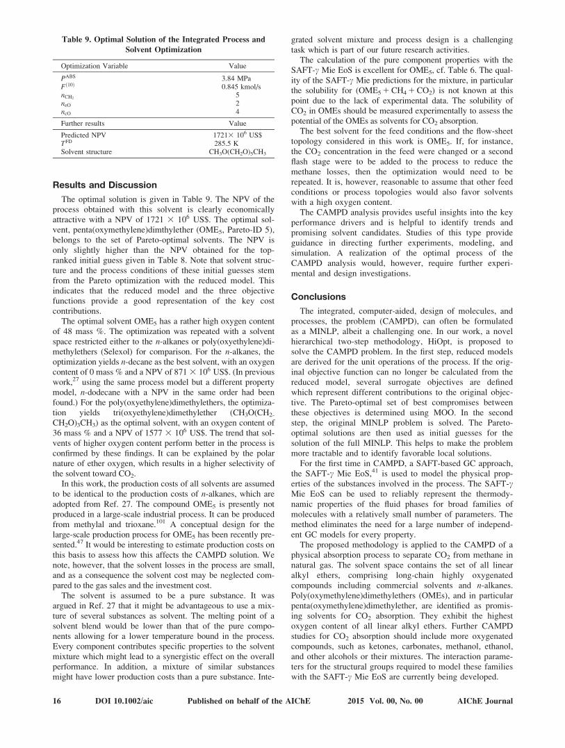
Results and Discussion

The optimal solution is given in Table 9. The NPV of theprocess obtained with this solvent is clearly economicallyattractive with a NPV of 1721 3 106 US$. The optimal sol-vent, penta(oxymethylene)dimthylether (OME5, Pareto-ID 5),belongs to the set of Pareto-optimal solvents. The NPV isonly slightly higher than the NPV obtained for the top-ranked initial guess given in Table 8. Note that solvent struc-ture and the process conditions of these initial guesses stemfrom the Pareto optimization with the reduced model. Thisindicates that the reduced model and the three objectivefunctions provide a good representation of the key costcontributions.

The optimal solvent OME5 has a rather high oxygen contentof 48 mass %. The optimization was repeated with a solventspace restricted either to the n-alkanes or poly(oxyethylene)di-methylethers (Selexol) for comparison. For the n-alkanes, theoptimization yields n-decane as the best solvent, with an oxygencontent of 0 mass % and a NPV of 871 3 106 US$. (In previouswork,27 using the same process model but a different propertymodel, n-dodecane with a NPV in the same order had beenfound.) For the poly(oxyethylene)dimethylethers, the optimiza-tion yields tri(oxyethylene)dimethylether (CH3O(CH2-

CH2O)3CH3) as the optimal solvent, with an oxygen content of36 mass % and a NPV of 1577 3 106 US$. The trend that sol-vents of higher oxygen content perform better in the process isconfirmed by these findings. It can be explained by the polarnature of ether oxygen, which results in a higher selectivity ofthe solvent toward CO2.

In this work, the production costs of all solvents are assumedto be identical to the production costs of n-alkanes, which areadopted from Ref. 27. The compound OME5 is presently notproduced in a large-scale industrial process. It can be producedfrom methylal and trioxane.101 A conceptual design for thelarge-scale production process for OME5 has been recently pre-sented.47 It would be interesting to estimate production costs onthis basis to assess how this affects the CAMPD solution. Wenote, however, that the solvent losses in the process are small,and as a consequence the solvent cost may be neglected com-pared to the gas sales and the investment cost.

The solvent is assumed to be a pure substance. It wasargued in Ref. 27 that it might be advantageous to use a mix-ture of several substances as solvent. The melting point of asolvent blend would be lower than that of the pure compo-nents allowing for a lower temperature bound in the process.Every component contributes specific properties to the solventmixture which might lead to a synergistic effect on the overallperformance. In addition, a mixture of similar substancesmight have lower production costs than a pure substance. Inte-

grated solvent mixture and process design is a challengingtask which is part of our future research activities.

The calculation of the pure component properties with theSAFT-c Mie EoS is excellent for OME5, cf. Table 6. The qual-ity of the SAFT-c Mie predictions for the mixture, in particularthe solubility for (OME5 1 CH4 1 CO2) is not known at thispoint due to the lack of experimental data. The solubility ofCO2 in OMEs should be measured experimentally to assess thepotential of the OMEs as solvents for CO2 absorption.

The best solvent for the feed conditions and the flow-sheettopology considered in this work is OME5. If, for instance,the CO2 concentration in the feed were changed or a secondflash stage were to be added to the process to reduce themethane losses, then the optimization would need to berepeated. It is, however, reasonable to assume that other feedconditions or process topologies would also favor solventswith a high oxygen content.

The CAMPD analysis provides useful insights into the keyperformance drivers and is helpful to identify trends andpromising solvent candidates. Studies of this type provideguidance in directing further experiments, modeling, andsimulation. A realization of the optimal process of theCAMPD analysis would, however, require further experi-mental and design investigations.

Conclusions

The integrated, computer-aided, design of molecules, andprocesses, the problem (CAMPD), can often be formulatedas a MINLP, albeit a challenging one. In our work, a novelhierarchical two-step methodology, HiOpt, is proposed tosolve the CAMPD problem. In the first step, reduced modelsare derived for the unit operations of the process. If the orig-inal objective function can no longer be calculated from thereduced model, several surrogate objectives are definedwhich represent different contributions to the original objec-tive. The Pareto-optimal set of best compromises betweenthese objectives is determined using MOO. In the secondstep, the original MINLP problem is solved. The Pareto-optimal solutions are then used as initial guesses for thesolution of the full MINLP. This helps to make the problemmore tractable and to identify favorable local solutions.

For the first time in CAMPD, a SAFT-based GC approach,the SAFT-c Mie EoS,41 is used to model the physical prop-erties of the substances involved in the process. The SAFT-cMie EoS can be used to reliably represent the thermody-namic properties of the fluid phases for broad families ofmolecules with a relatively small number of parameters. Themethod eliminates the need for a large number of independ-ent GC models for every property.

The proposed methodology is applied to the CAMPD of aphysical absorption process to separate CO2 from methane innatural gas. The solvent space contains the set of all linearalkyl ethers, comprising long-chain highly oxygenatedcompounds including commercial solvents and n-alkanes.Poly(oxymethylene)dimethylethers (OMEs), and in particularpenta(oxymethylene)dimethylether, are identified as promis-ing solvents for CO2 absorption. They exhibit the highestoxygen content of all linear alkyl ethers. Further CAMPDstudies for CO2 absorption should include more oxygenatedcompounds, such as ketones, carbonates, methanol, ethanol,and other alcohols or their mixtures. The interaction parame-ters for the structural groups required to model these familieswith the SAFT-c Mie EoS are currently being developed.

Table 9. Optimal Solution of the Integrated Process and

Solvent Optimization

Optimization Variable Value

PABS 3.84 MPaFð10Þ 0.845 kmol/snCH2

5neO 2ncO 4

Further results Value

Predicted NPV 17213 106 US$TFD 285.5 KSolvent structure CH3O(CH2O)5CH3


Acknowledgments

The authors would like to acknowledge financial supportfrom the Engineering and Physical Sciences Research Coun-cil (EPSRC) of the UK (EP/E016340 and EP/J014958). J.B.thanks Michael Bortz for fruitful discussions and the GermanAcademic Exchange Service (DAAD) for the provision of apost-doctoral scholarship. V.P. is thankful to the EPSRC forthe award of a PhD studentship and a Doctoral Prize Fellow-ship. S.G. is thankful for an Imperial College Scholarship.C.S.A. is grateful to the EPSRC for the award of a Leader-ship Fellowship (EP/J003840).

Literature Cited

1. Gani R, Achenie LEK, Venkatasubramanian V. Chapter 1: Introduction toCAMD. In: Achenie LEK, Gani R, Venkatasubramanian V, editors. Com-puter Aided Molecular Design: Theory and Practice, Vol. 12 of ComputerAided Chemical Engineering. Elsevier, Amsterdam, 2002:3–21.

2. Adjiman CS, Galindo A, Jackson G. Molecules matter: the expandingenvelope of process design. Comput-Aided Chem Eng. 2014;34:55–64.

3. Kossack S, Kraemer K, Gani R, Marquardt W. A systematic synthe-sis framework for extractive distillation processes. Chem Eng ResDes. 2008;86:781–792.

4. Papadopoulos AI, Linke P. Multiobjective molecular design for inte-grated process-solvent systems synthesis. AIChE J. 2006;52:1057–1070.

5. Papadopoulos AI, Stijepovic M, Linke P. On the systematic designand selection of optimal working fluids for organic rankine cycles.Appl Therm Eng. 2010;30:760–769.

6. Gani R, Jim�enez-Gonz�alez C, Constable DJC. Method for selectionof solvents for promotion of organic reactions. Comput Chem Eng.2005;29:1661–1676.

7. Struebing H, Ganase Z, Karamertzanis PG, Siougkrou E, Haycock P,Piccione PM, Armstrong A, Galindo A, Adjiman CS. Computer-aided molecular design of solvents for accelerated reaction kinetics.Nat Chem. 2013;5:952–957.

8. Siougkrou E, Galindo A, Adjiman CS. On the optimal design ofgas-expanded liquids based on process performance. Chem Eng Sci.2014;115:19–30.

9. Bardow A, Steur K, Gross J. Continuous-molecular targeting for integratedsolvent and process design. Ind Eng Chem Res. 2010;49:2834–2840.

10. Pistikopoulos EN, Stefanis SK. Optimal solvent design for environ-mental impact minimization. Comput Chem Eng. 1998;22:717–733.

11. Hamad AA, El-Halwagi MM. Simultaneous synthesis of mass separatingagents and interception networks. Chem Eng Res Des. 1998;76:376–388.

12. Hostrup M, Harper PM, Gani R. Design of environmentally benignprocesses: integration of solvent design and separation process syn-thesis. Comput Chem Eng. 1999;23:1395–1414.

13. Karunanithi AT, Achenie LEK, Gani R. A new decomposition-basedcomputer-aided molecular/mixture design methodology for thedesign of optimal solvents and solvent mixtures. Ind Eng Chem Res.2005;44:4785–4797.

14. Buxton A, Livingston AG, Pistikopoulos EN. Optimal design of sol-vent blends for environmental impact minimization. AIChE J. 1999;45:817–843.

15. Giovanoglou A, Barlatier J, Adjiman CS, Pistikopoulos EN,Cordiner JL. Optimal solvent design for batch separation based oneconomic performance. AIChE J. 2003;49:3095–3109.

16. Marcoulaki EC, Kokossis AC. On the development of novel chemi-cals using a systematic optimisation approach. Part II. Solventdesign. Chem Eng Sci. 2000;55:2547–2561.

17. Marcoulaki EC, Kokossis AC. On the development of novel chemi-cals using a systematic synthesis approach. Part I. Optimisationframework. Chem Eng Sci. 2000;55:2529–2546.

18. Eden MR, J€orgensen SB, Gani R, El-Halwagi MM. A novel frame-work for simultaneous separation process and product design. ChemEng Process: Process Intensification. 2004;43:595–608.

19. Eljack FT, Eden MR, Kazantzi V, Qin X, El-Halwagi MM. Simulta-neous process and molecular design—a property based approach.AIChE J. 2007;53:1232–1239.

20. Bommareddy S, Chemmangattuvalappil NG, Solvason CC, Eden MR.Simultaneous solution of process and molecular design problems usingan algebraic approach. Comput Chem Eng. 2010;34:1481–1486.

21. Gross J, Sadowski G. Perturbed-chain SAFT: an equation of statebased on a perturbation theory for chain molecules. Ind Eng ChemRes. 2001;40:1244–1260.

22. Lampe M, Gross J, Bardow A. Simultaneous process and workingfluid optimization for organic rankine cycles (ORC) using PC-SAFT.Comput- Aided Chem Eng. 2012;30:572–576.

23. Lampe M, Stavrou M, B€ucker HM, Gross J, Bardow A. Simultane-ous optimization of working fluid and process for organic Rankinecycles using PC-SAFT. Ind Eng Chem Res. 2014;53:8821–8830.

24. Gil-Villegas A, Galindo A, Whitehead PJ, Mills SJ, Jackson G, BurgessAN. Statistical associating fluid theory for chain molecules with attrac-tive potentials of variable range. J Chem Phys. 1997;106:4168–4186.

25. Galindo A, Davies LA, Gil-Villegas A, Jackson G. The thermodynam-ics of mixtures and the corresponding mixing rules in the SAFT-VRapproach for potentials of variable range. Mol Phys. 1998;93:241–252.

26. Pereira FE, Keskes E, Galindo A, Jackson G, Adjiman CS. Inte-grated design of CO2 capture processes from natural gas. In: Pistiko-poulos E, Galindo A, Kikkinides ES, Dua V, editors. ProcessSystems Engineering: Energy Systems Engineering. Weinheim:Wiley-VCH Verlag GmbH & Co. KGaA,. 2008:231–248.

27. Pereira FE, Keskes E, Galindo A, Jackson G, Adjiman CS. Inte-grated solvent and process design using a SAFT-VR thermodynamicdescription: high-pressure separation of carbon dioxide and methane.Comput Chem Eng. 2011;35:474–491.

28. Harper PM, Gani R, Kolar P, Ishikawa T. Computer-aided moleculardesign with combined molecular modeling and group contribution.Fluid Phase Equilib. 1999;158–160:337–347.

29. Papaioannou V, Adjiman CS, Jackson G, Galindo A. Group contribu-tion methodologies for the prediction of thermodynamic propertiesand phase behavior in mixtures. In: Pistikopoulos E, Georgiadis M,Dua V, Adjiman C, Galindo A, editors. Molecular systems engineering.Weinheim: Wiley-VCH Verlag GmbH & Co. KGaA, 2011:135–172.

30. Chapman WG, Gubbins KE, Jackson G, Radosz M. SAFT:Equation-of-state solution model for associating fluids. Fluid PhaseEquilib. 1989;52:31–38.

31. Chapman WG, Gubbins KE, Jackson G, Radosz M. New referenceequation of state for associating liquids. Ind Eng Chem Res. 1990;29:1709–1721.

32. M€uller EA, Gubbins KE. Molecular-based equations of state forassociating fluids: a review of SAFT and related approaches. IndEng Chem Res. 2001;40:2193–2211.

33. Paricaud P, Galindo A, Jackson G. Recent advances in the use ofthe SAFT approach in describing electrolytes, interfaces, liquid crys-tals and polymers. Fluid Phase Equilib. 2002;194–197:87–96.

34. Tan SP, Adidharma H, Radosz M. Recent advances and applicationsof statistical associating fluid theory. Ind Eng Chem Res. 2008;47:8063–8082.

35. Kontogeorgis GM, Folas GK. Thermodynamic Models for IndustrialApplications. Weinheim: Wiley-VCH, 2010.

36. McCabe C, Galindo A. SAFT associating fluids and fluid mixtures.In: Goodwin AR, Sengers J, Peters CJ, editors. Applied thermodynamicsof fluids. The Royal Society of Chemistry, London 2010, p. 215–279.

37. Perdomo FA, Perdomo L, Mill�an BM, Arag�on JL. Design andimprovement of biodiesel fuels blends by optimisation of theirmolecular structures and compositions. Chem Eng Res Des. 2014;92:1482–1494.

38. Lymperiadis A, Adjiman CS, Galindo A, Jackson G. A group contribu-tion method for associating chain molecules based on the statisticalassociating fluid theory (SAFT-c). J Chem Phys. 2007;127:234903.

39. Lymperiadis A, Adjiman CS, Jackson G, Galindo A. A generalisa-tion of the SAFT-c group contribution method for groups comprisingmultiple spherical segments. Fluid Phase Equilib. 2008;274:85–104.

40. Papaioannou V, Adjiman CS, Jackson G, Galindo A. Simultaneousprediction of vapour-liquid and liquid-liquid equilibria (VLE andLLE) of aqueous mixtures with the SAFT-c group contributionapproach. Fluid Phase Equilib. 2011;306:82–96.

41. Papaioannou V, Lafitte T, Avenda~no C, Adjiman CS, Jackson G,M€uller EA, Galindo A. Group contribution methodology based onthe statistical associating fluid theory for heteronuclear moleculesformed from mie segments. J Chem Phys. 2014;140:054107.

42. Lafitte T, Apostolakou A, Avenda~no C, Galindo A, Adjiman CS, M€ullerEA, Jackson G. Accurate statistical associating fluid theory for chain mole-cules formed from Mie segments. J Chem Phys. 2013;139:154504.

43. Douglas JM. A hierarchical decision procedure for process synthesis.AIChE J. 1985;31:353–362.

44. Smith R, Linnhoff B. The design of separators in the context ofoverall processes. Chem Eng Res Des. 1988;66:195–228.

45. Franke MB, Nowotny N, Ndocko EN, G�orak A, Strube J. Designand optimization of a hybrid distillation/melt crystallization process.AIChE J. 2008;54:2925–2942.


46. Han C, Kim M, Yoon ES. A hierarchical decision procedure for pro-ductivity innovation in large-scale petrochemical processes. ComputChem Eng. 2008;32:1029–1041.

47. Burger J, Str€ofer E, Hasse H. Production process for diesel fuelcomponents poly(oxymethylene) dimethyl ethers from methane-based products by hierarchical optimization with varying modeldepth. Chem Eng Res Des. 2013;91:2648–2662.

48. Burger J, Hasse H. Multi-objective optimization using reduced mod-els in conceptual design of a fuel additive production process. ChemEng Sci. 2013;99:118–126.

49. Petlyuk FB, Aventyan VS. Investigation of the rectification of three-component mixtures with infinite reflux. Theor Found Chem Eng.1971;5:499–507.

50. Serafimov LA, Zharov VT, Timofeev VS. Rectification of multicom-ponent mixtures. I. Topological analysis of liquid-vapour phase equi-librium diagrams. Acta Chim Acad Sci Hung. 1971;69:383–396.

51. Bekiaris N, Morari M. Multiple steady states in distillation: 1/1predictions, extensions, and implications for design, synthesis, andsimulation. Ind Eng Chem Res. 1996;35:4264–4280.

52. Ryll O, Blagov S, Hasse H. 1/1-Analysis of homogeneous distilla-tion processes. Chem Eng Sci. 2012;84:315–332.

53. G€uttinger TE, Dorn C, Morari M. Experimental study of multiplesteady states in homogeneous azeotropic distillation. Ind Eng ChemRes. 1997;36:794–802.

54. M€uller D, Marquardt W. Experimental verification of multiple steadystates in heterogeneous azeotropic distillation. Ind Eng Chem Res.1997;36:5410–5418.

55. G€uttinger TE. Multiple Steady States in Azeotropic and ReactiveDistillation. Ph.D. thesis, ETH Z€urich, 1998.

56. M€uller D. Modellierung und Analyse der Heteroazeotrop-Rektifikation im Wechselspiel zwischen Simulation und Experiment.Ph.D. thesis, RWTH Aachen, 1998.

57. Bortz M, Burger J, Asprion N, Blagov S, B€ottcher R, Nowak U,Scheithauer A, Welke R, K€ufer KH, Hasse H. Multi-criteria optimi-zation in chemical process design and decision support by navigationon pareto sets. Comput Chem Eng. 2014;60:354–363.

58. Ehrgott M, Gandibleux X. Approximative solution methods for mul-tiobjective combinatorial optimization. Top. 2004;12:1–63.

59. Fattahi A, Turkay M. �-OA for the solution of bi-objective general-ized disjunctive programming problems in the synthesis of nonlinearprocess networks. Comput Chem Eng. 2015;72:199–209.

60. Nannan NR, De Servi CM, van der Stelt T, Piero C, Bardow A. Anequation of state based on PC-SAFT for physical solvents composedof polyethylene glycol dimethylethers. Ind Eng Chem Res. 2013;52:18401–18412.

61. Qadir A, Chiesa M, Abbas A. In silico design of solvents for carboncapture with simultaneous optimisation of operating conditions. Int JGreenhouse Gas Control. 2014;30:179–187.

62. Papaioannou V. A Molecular-Based Group Contribution Equation ofState for the Description of Fluid Phase Behaviour and Thermody-namic Derivative Properties of Mixtures (SAFT-c Mie). Ph.D. thesis,Imperial College London, 2012.

63. Mie G. Zur kinetischen Theorie der einatomigen K€orper. Ann Phys.1903;316:657–697.

64. Jackson G, Chapman WG, Gubbins KE. Phase equilibria of associat-ing fluids: spherical molecules with multiple bonding sites, MolPhys. 1988;65:1–31.

65. Chapman WG, Jackson G, Gubbins KE. Phase equilibria of associat-ing fluids: chain molecules with multiple bonding sites. Mol Phys.1988;65:1057–1079.

66. Anderson CL, Siahaan A. Case study: membrane CO2 removal from nat-ural gas, Grissik gas plant, Sumatra, Indonesia. In: 55th Annual OklahomaUniversity Laurance Reid Gas Conditioning Conference, Norman,Oklahoma 2005; p. 51.

67. Kohl AL, Nielsen RB. Gas Purification. Houston: Gulf, PublishingCo., 1997.

68. McCabe C, Jackson G. SAFT-VR modelling of the phase equilibriumof long-chain n-alkanes. Phys Chem Chem Phys. 1999;1:2057–2064.

69. Paricaud P, Galindo A, Jackson G. Modeling the cloud curves andthe solubility of gases in amorphous and semicrystalline polyethyl-ene with the SAFT-VR approach and Flory theory of crystallization.Ind Eng Chem Res. 2004;43:6871–6889.

70. Holmes AS, Ryan JM, Price BC, Styring RE. Process improves acidgas separation. Hydrocarbon process. 1982;61:131–136.

71. Burger J, Siegert M, Str€ofer E, Hasse H. Poly(oxymethylene)dimethyl ethers as components of tailored diesel fuel: properties,synthesis and purification concepts. Fuel. 2010;89:3315–3319.

72. Papaioannou V, Lafitte T, Calado F, Sadeqzadeh M, Galindo A,Jackson G, Adjiman C, Pantelides C, Avaullee L, Duchet-SuchauxP, Fuentes J. Application of the SAFT-c Mie group contributionequation of state in the oil and gas industry. Ind Eng Chem Res. Inpreparation.

73. Dufal S, Papaioannou V, Sadeqzadeh M, Pogiatzis T, Chremos A,Adjiman CS, Jackson G, Galindo A. Prediction of thermodynamicproperties and phase behaviour of fluids and mixtures with theSAFT-c mie group-contribution equation of state. J Chem Eng Data.2014;59:3272–3288.

74. Ambrose D, Ellender JH, Sprake CHS, Townsend R. Thermody-namic properties of organic oxygen compounds-XLIII. Vapour pres-sures of some ethers. J Chem Thermo. 1976;8:165–178.

75. Fletcher DA, McMeeking RF, Parkin D. The United Kingdom chem-ical database service. J Chem Inf Comput Sci. 1996;36:746–749.

76. Cidlinsky J, Polak J. Saturated vapor pressures of some ethers. Col-lect Czechoslov Chem Commun. 1969;34:1317–1321.

77. Treszczanowicz T, Lu BCY. Isothermal vapour-liquid equilibria for11 examples of (an ether 1 a hydrocarbon). J Chem Thermo. 1986;18:213–220.

78. Timmermans J. Physico-Chemical Constants of Pure Organic Sub-stances, Vol. II. New York: Elsevier, 1965.

79. Wu HS, Sandler SI. Vapor-liquid equilibria for binary mixtures ofbutyl ether with 2-furaldehyde and 2-, 3-, and 4-heptanone. J ChemEng Data. 1988;33:316–321.

80. Kobe AK, Ravicz AE, Vohra SP. Critical properties and vapor pres-sures of some ethers and heterocyclic compounds. J Chem EngData. 1956;1:50–56.

81. Ryutani B. The solubility of acetylene in various organic solventsunder high pressure and at low temperature. IV. The solubility ofacetylene in Ethers. Nippon Kagaku Zasshi. 1960;81:1196–1201.

82. Chaudhari SK, Patil KR, Allep�us J, Coronas A. Measurement of thevapor pressure of 2,2,2-trifluoroethanol and tetraethylene glycol dimethylether by static method. Fluid Phase Equilib. 1995;108:159–165.

83. Boyd RH. Some physical properties of polyoxymethylene dimethylethers. J Polym Sci. 1961;50:133–141.

84. Riddick JA, Bunger WB, Sakano TK. Organic Solvents: PhysicalProperties and Methods of Purification, 4th ed. New York: WileyInterscience, 1986.

85. Obama M, Oodera Y, Kohama N, Yanase T, Saito Y, Kusano K.Densities, molar volumes, and cubic expansion coefficients of 78 ali-phatic ethers. J Chem Eng Data. 1985;30:1–5.

86. Lee MJ, Wei MC. Densities and viscosities of 2-butanone/-dibutylether, 2-picoline/2-butanone, and 2-picoline/water mixtures. J ChemEng Data. 1992;37:209–212.

87. Carvajal C, T€olle KJ, Smid J., Szwarc M. Studies of solvation phe-nomena of ions and ion pairs in dimethoxyethane and tetrahydrofu-ran. J Am Chem Soc. 1965;87:5548–5553.

88. Conesa A, Shen S, Coronas A. Liquid densities, kinematic viscosities,and heat capacities of some Ethylene glycol dimethyl ethers at tempera-tures from 283.15 to 423.15 K. J Thermophys. 1998;19:1343–1358.

89. Wu J, Xu Z, Liu Z, Wang B. Density and viscosity of saturated liq-uid dimethoxymethane from (218.15 to 383.15) K. J Chem EngData. 2005;50:966–968.

90. DIPPR. Thermophysical Properties Laboratory - Dippr Project 801,Department of Chemical Engineering, Brigham University, Pravo,Utah, 2012.

91. Kodama D, Kanakubo M, Kokubo M, Hashimoto S, Nanjo H, KatoM. Density, viscosity, and solubility of carbon dioxide in glymes.Fluid Phase Equilib. 2011;302:103–108.

92. Vilcu R, Gainar I, Anitescu G, Perisanu S. The solubility of CO2,H2 and N2 in dimethylether-diethyleneglycol. Rev Roum Chim. 1993;38:1169–1172.

93. Brignole EA, Chareton A, Laugier S, Richon D. Vapor-liquid equilib-rium data for the methane-methylal binary mixture between 273 and432 K up to the critical region. J Chem Eng Data. 1987;32:215–218.

94. Sastri SRS, Rao KK. A new group contribution method for predict-ing viscosity of organic liquids. Chem Eng J. 1992;50:9–25.

95. Marrero J, Gani R. Group-contribution based estimation of purecomponent properties. Fluid Phase Equilib. 2001;183–184:183–208.

96. Maranas CD. Optimal molecular design under property predictionuncertainty. AIChE J. 1997;43:1250–1264.

97. Process Systems Enterprise Ltd. gPROMS v. 3.5.3. Available at:http://www.psenterprise.com/, last accessed October 20, 2012.

98. Duran MA, Grossmann IE. An outer-approximation algorithm for aclass of mixed-integer nonlinear programs. Math Program. 1986;36:307–339.


http://www.psenterprise.com/

99. Viswanathan J, Grossmann IE. A combined penalty function andouter-approximation method for MINLP optimization. Comput ChemEng. 1990;14:769–782.

100. The MathWorks Inc. MATLAB v. R2013a. Available at: http://www.mathworks.com/, last accessed September 17, 2013.

101. Burger J, Str€ofer E, Hasse H. Chemical equilibrium and reactionkinetics of the heterogeneously catalyzed formation of poly (oxy-methylene) dimethyl ethers from methylal and trioxane. Ind EngChem Res. 2012;51:12751–12761.

102. Pereira FE, Jackson G, Galindo A, Adjiman CS. The HELD algo-rithm for multicomponent, multiphase equilibrium calculations withgeneric equations of state. Comput Chem Eng. 2012;36:99–118.

APPENDIX A

Composition of the Loaded Solvent for a Columnof Infinite Height

A rationale for the reduced model of the absorber is provided

in this Appendix. The generic absorption column considered is

shown schematically on the left panel of Figure 16. Stream F

denotes the inlet gas, Stream S is the inlet solvent, Stream R is

the outlet (clean) gas, and Stream L is the outlet (loaded) sol-

vent. Streams Li and Ri denote the liquid and vapor, respec-

tively, that leave stage i of the column. The column consists of

N stages. For every stage i, Ri and Li are in VLE. The compo-

nent mass balances around the overall column and around each

stage are

FFxF1FSxS 5FRxR1FLxL;

FRi11 xRi11 1FLi21 xLi21 5FRi xRi 1FLi xLi ; i ¼ 1; . . . ;N(A1)

where Fj denotes the molar flow rate of stream j, xj its composi-

tion vector. It follows from Eq. A1 that

FSxS2FRxRð Þ ¼ FLxL2FFxFð Þ ¼ FLi xLi 2FRi11 xRi11ð Þ¼ FPxP

(A2)

Thus, the “difference stream” P, defined as the difference

between the liquid and vapor stream at a given height in the col-

umn, is constant. Note that P is a virtual stream. Its flow rate FP

or some elements of its composition vector xP may be negative.

The compositions of the external and internal streams for a col-

umn with five stages are shown schematically in the ternary dia-

gram on the right panel of Figure 16, in which the tie lines of

VLE are represented. Both the pressure and the temperature are

assumed to be constant. The virtual stream P is located outside

the triangle, and is given as the intersection of the lines (FL) and

(RS). Starting from the clean gas R, the compositions of the inter-

nal streams can be constructed based on the VLE between the

gas Ri and liquid Li and Eq. A2: Ri and Li lie on the same tie

line and all lines through Ri11 and Li for any i intersect at P.

For the purpose of calculations with the reduced model in

our current work, the compositions of Streams R, F, and S are

known. The larger the number of stages present in the column,

the greater the achievable CO2 concentration of the loaded sol-

vent L. There is, however, a thermodynamic limit for the CO2

concentration of L: it can never exceed the CO2 concentration

of point L1 that lies on the tie line pointing to the feed F (cf.

Figure 16). Once the concentration L1 is reached in the liquid

phase, line (FP) coincides with the tie line through L1. The

compositions of both phases no longer change below the stage

at which this occurs. Such a stage is referred to as the pinch

point. When a column is assumed to be of infinite height

(N !1), as is the case for our reduced model, there must be

a pinch point in the column at which L 5 L1.

Comparison of Process Simulation ResultsObtained with Reduced and Full Model

An analysis of the accuracy of the reduced models used in

our work with respect to the full models is provided here. Using

the reduced model of the absorption column in process simula-

tions invokes the following steps:

1. Specify input parameters, including the compositionxð2Þ and flow rate Fð2Þ of the feed, the absorber pressurePABS, the process temperature T, and the desired purity ofproduct x

ð3ÞCH4

2. Solve a VLE flash at PABS, T under the constraint thatthe compositions of both phases xliq; xvap lie on a line pass-ing through xð2Þ in the composition space

t xvap2xliq

¼ xvap2xð2Þ� �

; t 2 R (A3)

3. Set xð4Þ ¼ xliq

4. Set xð3ÞCO2¼ 12x

ð3ÞCH4

5. Set xð10Þsolv ¼ 1

6. Use the overall mass balance

Fð2Þxð2Þ1Fð10Þxð10Þ ¼ Fð3Þxð3Þ1Fð4Þxð4Þ (A4)

to determine the flow rates of the streams leaving the column,

Fð3Þ and Fð4Þ, and the flow rate of fresh solvent Fð10Þ.A comparison of the concentrations calculated with the

reduced and the full model for the solvent penta(oxymethyle-

ne)dimethylether, one of the Pareto-optimal solvents uncov-

ered in our work, is shown in Figure 17, overlaid with the

phase envelope at the corresponding temperature and pressure.

The pressure in the absorption column and the purity of the

product gas stream are set to be identical in both models.

The temperature T in the reduced model is set equal to the

temperature Tð4Þ at the bottom of the absorption column

in the full model. The two models are in good agreement in

terms of the stream concentrations. The main differences are

that in the reduced model the lean solvent is purer and the

Figure 16. Determining the concentration of the loadedsolvent L for an absorption column compris-ing N 5 5 stages.

Left panel: schematic of the absorption column. F rep-

resents the feed gas, L the loaded solvent, R the clean

gas, and S the unloaded solvent. Vapor Ri and liquid Li

leaving stage i are in VLE. Right panel: Internal

streams for a 5-stage column shown on a ternary fluid-

phase diagram with the corresponding vapor-liquid

coexistence boundaries. Ri and Li lie on the same tie

line. The lines through Ri11 and Li, for any i, intersect

at one fixed point, P.


http://www.mathworks.com/

http://www.mathworks.com/

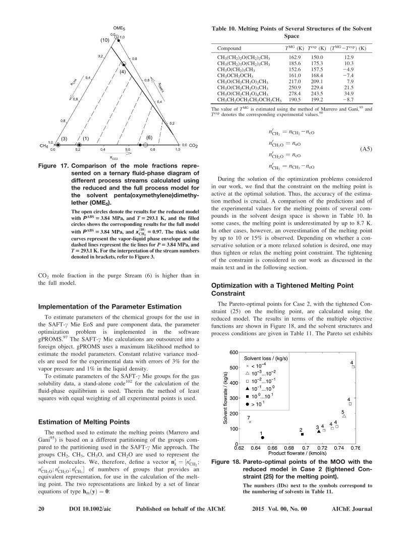
CO2 mole fraction in the purge Stream (6) is higher than in

the full model.

Implementation of the Parameter Estimation

To estimate parameters of the chemical groups for the use in

the SAFT-c Mie EoS and pure component data, the parameter

optimization problem is implemented in the software

gPROMS.97 The SAFT-c Mie calculations are outsourced into a

foreign object. gPROMS uses a maximum likelihood method to

estimate the model parameters. Constant relative variance mod-

els are used for the experimental data with errors of 3% for the

vapor pressure and 1% in the liquid density.

To estimate parameters of the SAFT-c Mie groups for the gas

solubility data, a stand-alone code102 for the calculation of the

fluid-phase equilibrium is used. Therein the method of least

squares with equal weighting of all experimental points is used.

Estimation of Melting Points

The method used to estimate the melting points (Marrero and

Gani95) is based on a different partitioning of the groups com-

pared to the partitioning used in the SAFT-c Mie approach. The

groups CH2, CH3, CH3O, and CH2O are used to represent the

solvent molecules. We, therefore, define a vector n0k ¼ ½n0CH2;

n0CH3O; n0CH2O; n0CH3� of numbers of groups that provides an

equivalent representation, for use in the calculation of the melt-

ing point. The two representations are linked by a set of linear

equations of type hmðyÞ ¼ 0:

n0CH2¼ nCH2

2ncO

n0CH3O ¼ neO

n0CH2O ¼ ncO

n0CH3¼ nCH3

2neO

(A5)

During the solution of the optimization problems considered

in our work, we find that the constraint on the melting point is

active at the optimal solution. Thus, the accuracy of the estima-

tion method is crucial. A comparison of the predictions and of

the experimental values for the melting points of several com-

pounds in the solvent design space is shown in Table 10. In

some cases, the melting point is underestimated by up to 8.7 K.

In other cases, however, an overestimation of the melting point

by up to 10 or 15% is observed. Depending on whether a con-

servative solution or a more relaxed solution is desired, one may

thus tighten or relax the melting point constraint. The tightening

of the constraint is considered in our work as discussed in the

main text and in the following section.

Optimization with a Tightened Melting PointConstraint

The Pareto-optimal points for Case 2, with the tightened Con-

straint (25) on the melting point, are calculated using the

reduced model. The results in terms of the multiple objective

functions are shown in Figure 18, and the solvent structures and

process conditions are given in Table 11. The Pareto set exhibits

Figure 17. Comparison of the mole fractions repre-sented on a ternary fluid-phase diagram ofdifferent process streams calculated usingthe reduced and the full process model forthe solvent penta(oxymethylene)dimethy-lether (OME5).

The open circles denote the results for the reduced model

with PABS 5 3.84 MPa, and T 5 293.1 K, and the filled

circles shows the corresponding results for the full model

with PABS 5 3.84 MPa, and xð10ÞCH4

5 0.97. The thick solid

curves represent the vapor-liquid phase envelope and the

dashed lines represent the tie lines for P 5 3.84 MPa, and

T 5 293.1 K. For the interpretation of the stream numbers

denoted in brackets, refer to Figure 3.

Table 10. Melting Points of Several Structures of the Solvent

Space

Compound TMG (K) Texp (K) ðTMG2TexpÞ (K)

CH3(CH2)2O(CH2)2CH3 162.9 150.0 12.9CH3(CH2)3O(CH2)3CH3 185.6 175.3 10.3CH3O(CH2)3CH3 152.6 157.5 24.9CH3OCH2OCH3 161.0 168.4 27.4CH3O(CH2CH2O)2CH3 217.0 209.1 7.9CH3O(CH2CH2O)3CH3 250.9 229.4 21.5CH3O(CH2CH2O)4CH3 278.4 243.5 34.9CH3CH2OCH2CH2OCH2CH3 190.5 199.2 28.7

The value of TMG is estimated using the method of Marrero and Gani,95 andTexp denotes the corresponding experimental values.90

Figure 18. Pareto-optimal points of the MOO with thereduced model in Case 2 (tightened Con-straint (25) for the melting point).

The numbers (IDs) next to the symbols correspond to

the numbering of solvents in Table 11.


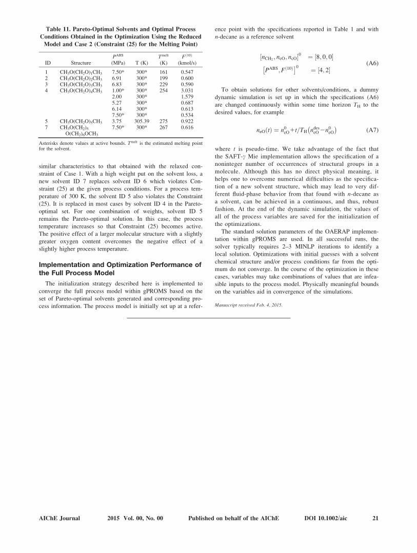
similar characteristics to that obtained with the relaxed con-

straint of Case 1. With a high weight put on the solvent loss, a

new solvent ID 7 replaces solvent ID 6 which violates Con-

straint (25) at the given process conditions. For a process tem-

perature of 300 K, the solvent ID 5 also violates the Constraint

(25). It is replaced in most cases by solvent ID 4 in the Pareto-

optimal set. For one combination of weights, solvent ID 5

remains the Pareto-optimal solution. In this case, the process

temperature increases so that Constraint (25) becomes active.

The positive effect of a larger molecular structure with a slightly

greater oxygen content overcomes the negative effect of a

slightly higher process temperature.

Implementation and Optimization Performance ofthe Full Process Model

The initialization strategy described here is implemented to

converge the full process model within gPROMS based on the

set of Pareto-optimal solvents generated and corresponding pro-

cess information. The process model is initially set up at a refer-

ence point with the specifications reported in Table 1 and with

n-decane as a reference solvent

nCH2; neO; ncO½ �0 ¼ 8; 0; 0½ �

PABS;Fð10Þ� �0 ¼ 4; 2½ �(A6)

To obtain solutions for other solvents/conditions, a dummy

dynamic simulation is set up in which the specifications (A6)

are changed continuously within some time horizon TH to the

desired values, for example

neOðtÞ ¼ n0eO1t=TH ndes

eO 2n0eO

(A7)

where t is pseudo-time. We take advantage of the fact that

the SAFT-c Mie implementation allows the specification of a

noninteger number of occurrences of structural groups in a

molecule. Although this has no direct physical meaning, it

helps one to overcome numerical difficulties as the specifica-

tion of a new solvent structure, which may lead to very dif-

ferent fluid-phase behavior from that found with n-decane as

a solvent, can be achieved in a continuous, and thus, robust

fashion. At the end of the dynamic simulation, the values of

all of the process variables are saved for the initialization of

the optimizations.

The standard solution parameters of the OAERAP implemen-

tation within gPROMS are used. In all successful runs, the

solver typically requires 2–3 MINLP iterations to identify a

local solution. Optimizations with initial guesses with a solvent

chemical structure and/or process conditions far from the opti-

mum do not converge. In the course of the optimization in these

cases, variables may take combinations of values that are infea-

sible inputs to the process model. Physically meaningful bounds

on the variables aid in convergence of the simulations.

Manuscript received Feb. 4, 2015.

Table 11. Pareto-Optimal Solvents and Optimal Process

Conditions Obtained in the Optimization Using the Reduced

Model and Case 2 (Constraint (25) for the Melting Point)

ID StructurePABS

(MPa) T (K)Tmelt

(K)Fð10Þ

(kmol/s)

1 CH3O(CH2O)1CH3 7.50* 300* 161 0.5472 CH3O(CH2O)2CH3 6.91 300* 199 0.6003 CH3O(CH2O)3CH3 6.83 300* 229 0.5904 CH3O(CH2O)4CH3 1.00* 300* 254 3.031

2.00 300* 1.5795.27 300* 0.6876.14 300* 0.6137.50* 300* 0.534

5 CH3O(CH2O)5CH3 3.75 305.39 275 0.9227 CH3O(CH2)5

O(CH2)6OCH3

7.50* 300* 267 0.616

Asterisks denote values at active bounds. Tmelt is the estimated melting pointfor the solvent.


a hierarchical method to integrated solvent and … hierarchical method to integrated solvent and...

Documents