a hierarchical verification of the ieee-754 table-driven...
TRANSCRIPT

A Hierarchical Verification of theIEEE-754 Table-Driven Floating-Point
Exponential Function using HOL
Amr Talaat Abdel-Hamid
A Thesis
in
The Department
of
Electrical and Computer Engineering
Presented in Partial Fulfilment of the Requirements
for the Degree of Master of Applied Science at
Concordia University
Montréal, Québec, Canada
April 2001
@Amr T. Abdel-Hamid, 2001

CONCORDIA UNIVERSITY
School of Graduate Studies
This is to certify that the thesis prepared
By: Amr Talaat Abdel-Hamid
Entitled: A Hierarchical Verification of The IEEE-754 Table-Driven Floating-Point Exponential Function using HOL
and submitted in partial fulfilment of the requirements for the degree of
Master of Applied Science (Electrical and Computer Engineering)
complies with the regulations of the University and meets the accepted standards withrespect to originality and quality.
Signed by the final examining committee:
_________________________
_________________________
_________________________
_________________________
Approved by _______________________________________________________Chair of Department or Graduate Program Director
___________________________________________Dean of Faculty

iii
Abstract
A Hierarchical Verification of the IEEE-754 Table-Driven
Floating-Point Exponential Function using HOL
The IEEE-754 floating-point standard, used in nearly all floating-point applications, is
considered one of the most important standards. Deep datapath and algorithm complexity
have made the verification of such floating-point units a very hard task. Most simulation
and reachability analysis verification tools fail to verify a circuit with a deep datapath like
most industrial floating-point units. Theorem proving, however, offers a better solution to
handle such verification.
In this thesis, we have formalized and verified a hardware implementation of the
IEEE-754 Table-Driven floating-point exponential function algorithm using the HOL the-
orem prover. The high ability of abstraction in the HOL verification system allows its use
for the verification task over the whole design path of the circuit, starting from the gate
level implementation of the circuit up to a higher level behavioral specification. To
achieve this goal, we have used both hierarchical and modular approaches for modeling
and verifying the floating-point exponential function in HOL.

iv
Acknowledgments
I could not have completed this thesis without the assistance of many people. First and
foremost, I would like to express my thanks and indebtedness to my supervisor Dr. Sofiène
Tahar for his constructive technical advice, financial support, constant guidance, and
encouragement throughout this work. Dr. Tahar has always given me a real example of how
a researcher should be.
Throughout my study in Concordia many people have encouraged and helped me
through many obstacles. I have enjoyed studying and working with my colleagues in the
HVG group in Concordia University, wishing to thank all of them for their support and the
nice time we have spent together. In Particular, I would like to express my special gratitude
to Dr. Skander Kort for his valuable discussions during my research work.
I owe gratitude for the Inter-university center in computer architecture and VLSI
(GRIAO) for the financial support they provided to this work in order to be completed
through out the GRIAO graduate scholarship program.
Also, I would like to give my gratitude to Mr. Kamal, my preparatory mathematics
teacher, who introduced the first mathematical proof in my life and made me really enjoy
it.
If not for the love and support of my family, Mom, Dad, and my only sister, I would not
be able to complete my M.A.Sc. program. Their life time support and encouragement has
provided the basic foundation of any success I will ever achieve.

v
Dedication
To my family,
Mom, Dad,
and my only Sister

vi
Table of Contents
List of Figures vii
List of Tables viii
Chapter 1 Introduction 11.1 Formal Hardware Verification.............................................................................. 1
1.1.1 Decision Diagram Based Methods............................................................ 51.1.2 Theorem Proving....................................................................................... 6
1.2 Floating-Point Numbers and the IEEE-754 Standard .......................................... 71.2.1 Floating-Point Numbers ............................................................................ 71.2.2 IEEE-754 Floating-Point Standard ......................................................... 10
1.3 Related Work...................................................................................................... 131.4 Scope of this Thesis ........................................................................................... 15
Chapter 2 Hardware Verification and the HOL System 182.1 Higher-Order Logic and HOL............................................................................ 18
2.1.1 Higher-Order Logic................................................................................. 182.1.2 The HOL98 System................................................................................. 19
2.2 Hardware Verification using HOL ..................................................................... 222.2.1 Modeling Hardware Behavior using HOL.............................................. 222.2.2 Performing Proofs using the HOL System.............................................. 23
Chapter 3 Formal Modeling of the Exponential Function 283.1 Table-Driven Exponential Function (Mathematical Background) ..................... 283.2 Table Driven Exponential Function Specification.............................................. 313.3 Implementation of IEEE-754 Exponential Function.......................................... 39
Chapter 4 Verification of The Exponential Function Using HOL 464.1 Verification Methodology................................................................................... 46
4.2.1 Verification and Hardware Design Path .................................................. 464.2.2 Exponential Function Verification........................................................... 48
4.2 Formal Verification of the Exponential Function............................................... 514.3 Experimental Results ......................................................................................... 56
Chapter 5 Conclusions and Future Work 58
Bibliography 61
vii
List of Figures
Figure 1.1: Formal Verification Approach ..................................................................... 2
Figure 1.2: Typical Representation of a Floating-Point Number ................................... 8
Figure 1.3: Sub-ranges and Special Values in Floating-Point Number Representations 9
Figure 2.1: Hierarchy of Theories ................................................................................ 21
Figure 2.2: Circuit Module as a Black Box ................................................................. 22
Figure 2.3: Composition of Modules ........................................................................... 23
Figure 2.4: HOL Proof Procedure for Hardware Verification ...................................... 26
Figure 3.1: The Modular Organization of Exponential Function Specification .......... 33
Figure 3.2: The Behavioral Specification for the Exponential Function in “while-lan-
guage” [2] .................................................................................................... 34
Figure 3.3: Specification of the M-J Module (M_J_Spec) .......................................... 35
Figure 3.4: Specifying the Floating-Point Multiplier .................................................. 36
Figure 3.5: distrib_Spec and collect_Spec and their Usage in the Modeling Process . 37
Figure 3.6: Top-level VHDL Implementation Built in Synopsys Design Analyzer .... 41
Figure 3.7: Synthesis of the M_J Module VHDL Implementation with Synopsys Design
Analyzer ...................................................................................................... 42
Figure 4.1: Design Stages and Errors [24] ................................................................... 46
Figure 4.2: Verification Stages of the Exponential Function ....................................... 49
Figure 4.3: Hierarchical Verification Approach ........................................................... 50

viii
List of Tables
Table 1.1 Features of the ANSI/IEEE Standard Floating-Point Representation .......... 11
Table 4.1 Abstraction Levels in Circuit Design [24] ................................................... 47
Table 4.2 Verification Times of Different System Modules ......................................... 57
1
Chapter 1
Introduction
The verification of floating-point circuits has always been an important part of processor
verification. The importance of arithmetic circuit verification was illustrated by the famous
floating-point division bug in Intel’s Pentium processor [20]. Floating-point algorithms are
usually very complicated. They are composed of many modules where the smallest flaw in
design or implementation can cause a very hard-to-discover bug, as occurred in Intel’s case.
Traditional approaches to verifying floating-point circuits are based on simulation.
However, these approaches cannot exhaustively cover the input space of the circuits.
1.1 Formal Hardware Verification
Hardware designs are getting larger and larger, more complex everyday. With a fast
moving market like consumer electronics, where short time-to-market is sometimes the
only difference between success and failure of a product,Fast, Efficient,andFully Trusted
approaches should be adopted for testing these products. It would be a lot better if these
methods give a full coverage of these products because, the smallest design flaw in
hardware can be nearly lethal to this product. Full coverage and less design errors is what
Formal Hardware Verificationis trying to offer.
Formal Hardware Verification: “is the proof that a circuit or a system (the
implementation) behaves according to a given set of requirements (the specification).”[24]
Formal verification has theFull Coverageadvantage over any other testing method.
This can meanreal fault free products if it was used in the whole design path.As indicated

2
from the definition, all Formal Verification approaches are composed of three parts:first,
the circuit (system) under investigation (called the implementation);second,the set of
requirements this circuit should obey (called thespecification); and finally, the formal
verification toolwhich is responsible for the verification process.
Figure 1.1: Formal Verification Approach
As shown in Figure 1.1, these three parts interact with each other to ensure system
correctness. This can be achieved by modeling both the implementation and the
specification in the tool, in some cases the tool is responsible for modeling too, and then
the tool uses one of the formal verification algorithms to check the correctness of the
system or in some cases also to give a kind of trace (calledcounter example) to where the
error is.
Formal methods have long been developed and advocated within the computing science
research community as they provide sound mathematical foundation for the specification,
implementation and verification of computer systems. These methods exploit
representations with formally defined semantics in order to describe abstractly
(independent of details of implementation) the desired functional behavior of a system [24].
Implementation Specification
Formal Verification Tool
Correct
Not Correct(Counter Example)

3
Such formalization methods provide precise and unambiguous system specifications which
can be checked for completeness and internal logical consistency. The mathematical nature
of these specifications enable reasoning about consistency (i.e., whether the system
dynamics is consistent with system’s static properties) and the deduction of consequences
of the specification. These can be checked against the user’s expectations and used to
generate tests for the system implementation.
Simulation, although widely used as a way for testing, could never give the verification
coverage needed. There are two full coverage approaches, brute-force and special-purpose
simulation [4], which even fail to give a fair coverage ratio for a moderate design. Usually
a test pattern (vector) is generated either randomly or by an algorithm. This tries to cover
the areas that could be faulty and check that the design is working correctly. But this
process, although less time consuming, is also less accurate, because sometimes faults
occur where they are least expected. Directive test benches, and random test benches are
the ways adopted by simulation to get over these problems, but it is becoming clear that the
“quality” of the validation achieved by traditional simulation is rapidly deteriorating as
VLSI technology progresses.
Specifications in an executable formal language allow direct simulations (animations)
of system behavior, giving early feedback to be compared with user requirements before
full system development is begun. Equally important in the system development process, a
formal specification which is a yardstick against which to verify implementations or
implementation steps through mathematical proof of the equivalence of abstract and
concrete representations of system operations or data structures [24]. A formally based
development methodology requires that a mathematical theory of the desired system be

4
created, documented and analyzed. This foundation activity entails a greater proportion of
time and effort being invested in the initial pre-design phases of system development than
is now commonly the case.
Thanks to the rigorous discipline imposed by these methods, system development
phases are rendered less error-prone, more systematic and amenable to computer
assistance, and hence higher quality products are achieved. Thus, formal verification is
proposed as a method to help certify hardware and software, and consequently, to increase
confidence in new designs. Formally verifying designs may be cost effective in “safety
critical” applications, for systems in high volume or remotely placed systems, and for
systems that will go through frequent redesign because of changes in technology. Recently,
formal verification has been considered as a powerful complementary approach to
simulation and has made exciting progress.
Formal Verification is not the golden rule in circuit testing because of some limitations
[27]. A correctness proof cannot guarantee that the real device will never malfunction; the
design of the device may be proved correct, but the hardware actually built can still behave
in a way unintended by the designer (this is the case for simulation too). Wrong
specifications can play a major role in this, because it has been verified that the system will
function as specified, but it has not been verified that it will work correctly. Defects in
physical fabrication can cause this problem too. In formal verification amodelof the design
is verified, not the real physical implementation. Therefore, a fault in the modeling process
can givefalse negatives(errors in the design which do not exist). Although sometimes, the
fault covers some real errors.
5
Formal verification can generally be divided into two main categories [9]:reachability
analysis,anddeductive methods.Model checkers and equivalence checkers are examples
of the first approach. Many different theorem provers (such as HOL [12]) have been used
for deductive verification.
1.1.1 Decision Diagram Based Methods
Reachability analysis approaches are internally categorized into two main flows:Model
checking, and equivalence checking.
Model checking: In this approach, a circuit is described as a state machine with
transitions to describe the circuit behavior. The specifications are described as properties
that the machine should or should not satisfy. Traditionally, model checkers used explicit
representations of the state transition graph, for all but the smallest state machines. To
overcome this capacity limitation, different representations of BDD’s (Binary Decision
Diagrams) are used to represent the state transition graphs and this allows model checkers
(such as SMV [26], and VIS [5]) to verify systems with as many as 10-100 states, much
larger than that can be verified using an explicit state representation technique. However,
these model checkers still have the state explosion problem (i.e., BDD size explosion)
while verifying large circuits [9].
Equivalence checking: In recent years, many CAD vendors offer equivalence checking
tools for design verification. For example, the partial list of equivalence checkers are
Formality (from Synopsys [39]), and MDG [10] (University of Montreal). These tools
perform logic equivalence checking of two circuits based on structural analysis. The
common assumption used in the equivalence checking is that two circuits have identical
state encoding (latches) [9]. With this assumption, only the equivalence of the

6
combinational portions of two circuits must be checked. These tools cant handle large
designs with similar structures. However, these tools cannot handle the equivalence of
designs with no structure similarity. Another drawback of equivalence checkers is that they
all need golden circuits as the reference to be compared with. However, the correctness of
golden circuits is still questionable [9].
The major advantage of the reachability analysis verification approaches isautomation.
The machine (tool) is usually responsible for building the whole model and automatically
verifying either the equivalence or a property. But reachability analysis verification has two
main drawbacks which affect it, specially in the field of floating-point verification.First is
the state explosion problem, where large designs (or deep datapaths) saturate the tool,
stopping it from continuing the verification process.Second,is the problematic description
of specifications as properties, specially in model checking, this description needs
experience and sometimes may not give full system coverage.
Also, to verify floating-point arithmetic circuits, model checkers encounter more
difficulties as noted in [8].First, the specification languages are not powerful enough to
express arithmetic properties; for arithmetic circuits, the specifications must be expressed
as Boolean functions, which is not suitable for complex circuits.Second, these model
checkers cannot represent arithmetic circuits efficiently in their models.
1.1.2 Theorem Proving
With theorem proving, an implementation and its specification are usually expressed as
first-order or higher-order logic formulas. Their relationship, stated as equivalence or
implication, is regarded as a theorem to be proven within the logic system, using axioms
7
and inference rules. Thus, theorem proving is a powerful verification technique. It can
provide a unifying framework for various verification tasks at different hierarchical levels.
However, the task of proving complex theorems needs expertise. A theorem prover or
proof checker is a tool developed to partially automate the proof process or to check a
manual proof. Theorem proving systems are being widely used on an industrial scale for
hardware and software verification. Some of the well-known ones are HOL (Higher Order
Logic) [12], and PVS (Prototype Verification System) [14].
Theorem proving is considered a very strong verification tool because mathematical
formulas can express nearly all design levels. The proof procedures are very efficient if
they are constructed by experts. Also, hierarchical modeling is used to give theorem
provers nearly unlimited power; especially in handling deep datapath designs, which can
be modeled efficiently, using a hierarchy in most of the common theorem provers.
The main problem with theorem proving techniques is the lack of expertise and
documentation. It takes a considerably long time to learn theorem proving techniques.
Also, there is a strong need for libraries of specifications to be established, and more
automated tools and approaches.
1.2 Floating-Point Numbers and the IEEE-754 Standard
1.2.1 Floating-Point Numbers
Computers were originally built asfast, reliable, andaccuratecomputing machines. It
does not matter how large computers get, one of their main tasks will be to always perform
computation. The history of computer arithmetic is always interwined with that of digital
computers. In all microprocessor based computers, the Arithmetic Logic Unit (ALU) is one

8
of the units that takes most of the design effort to introduce more accurate and faster
techniques.
Most of these computations need real numbers as an essential category in any real world
calculations. Real numbers arenot finite, therefore no finite representation method is
capable of representing all real numbers, even within a small range. Thus, most real values
will have to be represented in an approximate manner. Various methods can be used for this
representation [35]:
1.Fixed-point number systems: offer limited range and/or precision. Computations must be
“scaled” to ensure that values remain representable and that they do not lose much
precision
2. Rational number systems: approximate a real value by the ratio of two integers, and lead
to difficult arithmetic operations.
3. Floating-point number systems: represent numbers in 3 fields (sign, exponent and
mantissa), and is the most common approach which will be discussed in detail shortly.
4. Logarithmic numbers systems: represent numbers by their signs and logarithms,
attractive for applications needing low precision and wide dynamic range, considered as
a limited special case of floating-point representation.
Figure 1.2: Typical Representation of a Floating-Point Number
A typical floating-point number representation (shown in Figure 1.2) is composed of
four main components [35]: the sign, the significant (also called mantissa)s, the exponent
+/- s: Significante: Exponent

9
baseb, and the exponente. The exponent baseb is usually implied (not explicitly
represented) and is usually a power of 2, except of course in the case of decimal arithmetic.
This number then is represented as follows:
A main point to observe is that there are two signs involved in a floating-point number:
1. The number signindicates a positive or negative floating-point number and is usually
represented by a separate sign bit (signed-magnitude convention).
2. The exponent signis embedded in the biased exponent and it indicates mainly a large or
small number. If the bias is a power of 2, the exponent is the complement of its most
significant bit.
The use of biased exponent format has virtually no effect on the speed or cost of
exponent arithmetic (addition/subtraction) [35], given the small number of bits involved. It
does, however, facilitate zero detection (zero will be represented with the smallest biased
exponent of 0 and an all-zero significant) and magnitude comparison (we compare
normalized floating-point numbers as if they were integers).
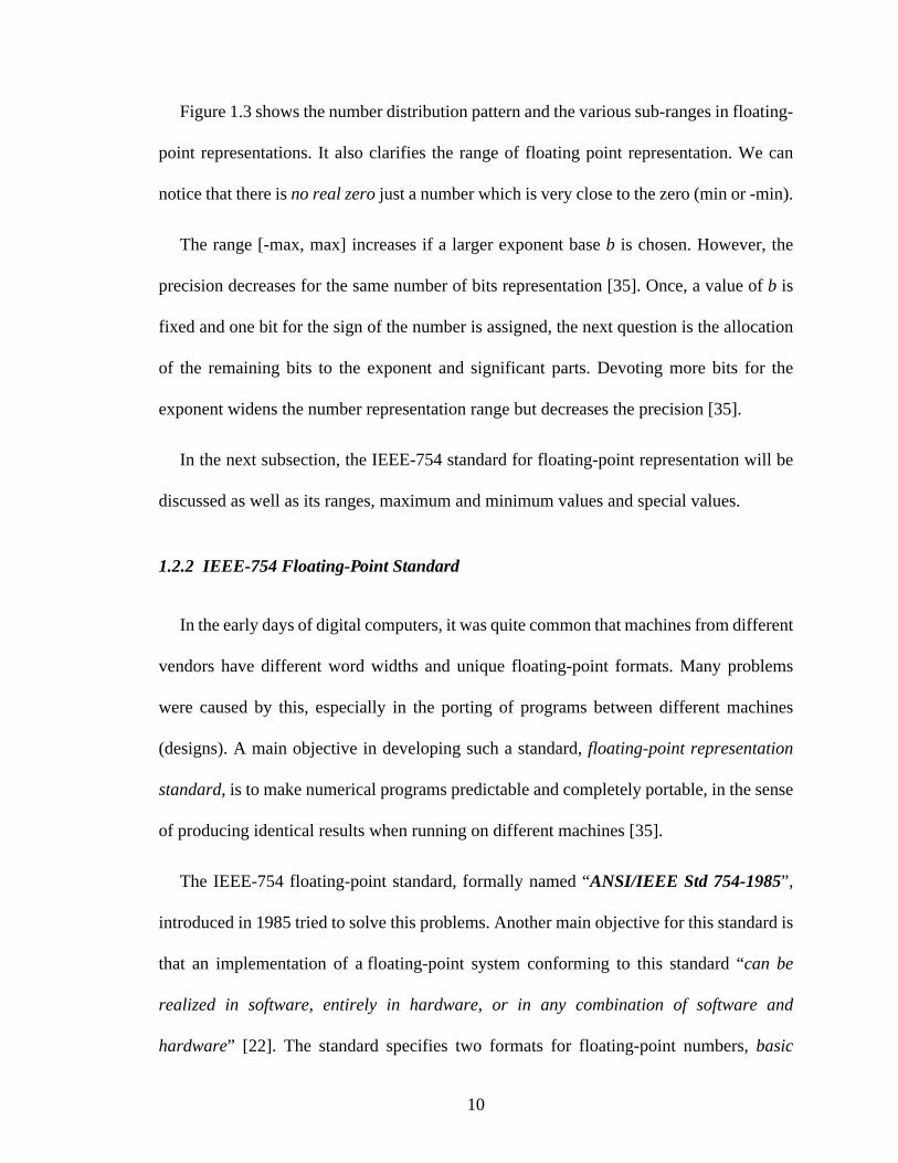
The range of values in a floating-point number representation format (shown in Figure
1.3) is composed of the intervals [- max, -min] and [ min, max], where:
Figure 1.3: Sub-ranges and Special Values in Floating-Point Number Representations
s be×±
max SIGmax biasEXPmax×=
min SIGmin biasEXPmin×=
+-
UnderflowOverflow Overflow
0 .... ........DenserDenser SparserSparser
10
Figure 1.3 shows the number distribution pattern and the various sub-ranges in floating-
point representations. It also clarifies the range of floating point representation. We can
notice that there isno real zerojust a number which is very close to the zero (min or -min).
The range [-max, max] increases if a larger exponent baseb is chosen. However, the
precision decreases for the same number of bits representation [35]. Once, a value ofb is
fixed and one bit for the sign of the number is assigned, the next question is the allocation
of the remaining bits to the exponent and significant parts. Devoting more bits for the
exponent widens the number representation range but decreases the precision [35].
In the next subsection, the IEEE-754 standard for floating-point representation will be
discussed as well as its ranges, maximum and minimum values and special values.
1.2.2 IEEE-754 Floating-Point Standard
In the early days of digital computers, it was quite common that machines from different
vendors have different word widths and unique floating-point formats. Many problems
were caused by this, especially in the porting of programs between different machines
(designs). A main objective in developing such a standard,floating-point representation
standard, is to make numerical programs predictable and completely portable, in the sense
of producing identical results when running on different machines [35].
The IEEE-754 floating-point standard, formally named “ANSI/IEEE Std 754-1985”,
introduced in 1985 tried to solve this problems. Another main objective for this standard is
that an implementation of a floating-point system conforming to this standard “can be
realized in software, entirely in hardware, or in any combination of software and
hardware” [22]. The standard specifies two formats for floating-point numbers,basic

11
(single precision) andextended(double precision), it also specifies the basic operations for
both formats which are addition, subtraction, multiplication, division, square root,
remainder, and comparison of operations. Then different conversions are needed, as integer
to floating-point, basic to extended and vice versa. Finally, it describes the different
floating-point exceptions and their handling, including non-numbers (NaNs) [22].
Table 1.1 Features of the ANSI/IEEE Standard Floating-Point Representation
Table 1.1 summarizes the most important features of IEEE floating-point standard. Zero
can not be presented with a normalized significant, thus, a special code was assigned to it,
Zero has all zero representation with either + or - sign. Also, special codes where needed
to represent other exceptions as NaN (not-a-number), and . The NaN is useful for
representingundefined results as 0/0.
Feature Single Double
Word width, bits 32 64
Significant bits 23 + 1 hidden 52 + 1 hidden
Significant range
Exponent bits 8 11
Exponent bias 127 1023
Zero e + bias = 0, f = 0 e + bias = 0, f = 0
Infinity e + bias = 255, f = 0 e + bias = 2047, f = 0
Not-a-number (NAN) e + bias = 255, f 0 e + bias = 2047, f 0
Minimum
Maximum
1 2 2 23––,[ ] 1 2 2 52––,[ ]
0±( )
∞±( )
≠ ≠
2 126– 1.2 10 38–×≈ 2 126– 2.2 10 308–×≈
2128 3.4 1038×≈ ≈ 21024 1.8 10308×≈ ≈
∞±

12
The standard has adopted the hidden (implicit) approach to save one bit in the
representation, contributing to increasing the precision without taking up space [35]. This
can be done by always representing the floating-point numbers innormalizedform, starting
with 1 in the most significant bit of the mantissa (significant). Therefore one can omit this
1 in storing the number. Denormals, or denormalized values are defined as numbers
without a hidden 1 and with the smallest possible exponent. These numbers where provided
to decrease the effect in case of underflow. This provision can lead to a high speed and cost
overhead, so it was offered optionally.
In this thesis, we have used only the single precision format of the standard. Table 1.1
shows that this format uses 8 bits for exponent with abiasof 127. Twenty-three bits are
used as significant (mantissa) with one hidden bit, which will always be concatenated with
one at demoralizing phases. We did not use denormal format and we have also defined
certain ranges for operations to protect our function from overflow and undesired inputs.
The standard defined only five arithmetic operations:Addition, Subtraction,
Multiplication, DivisionandSquare root. Many implementations are still needed for a real
computation scheme, for instance in a microprocessor floating-point computation unit.
This lead to a lot of work to produce accurate and fast algorithms used in computing
different floating-point operations. One of which was the work of Tang [40], who used
polynomial expansion to produce a new method to calculate the floating-point exponential
function; which will be discussed thoroughly in Chapter 3.

13
1.3 Related Work
There exists some related work on the verification of floating-point algorithms and
designs in the open literature.
Miner [29] formalized the IEEE-854 floating-point standard in PVS. He defined the
relation between floating-point numbers and real numbers, rounding, and some arithmetic
operations on both finite and infinite operands. He used this formalization to verify abstract
mathematical descriptions of the main operations and their relation to the corresponding
floating-point implementations. This paper is one of the earliest works in formalization of
floating-point standards using theorem proving. It described a large portion of the IEEE-
754 standard but did not cover all of it.
Carreno [7] formalized the same, IEEE-854 standard, in HOL. He interpreted the lexical
descriptions in the standard into mathematical conditional descriptions and organized them
in tables; then these table were formalized in HOL. He discussed different standard aspects
such as precisions, exceptions and traps, and many other arithmetic operations such as
addition, multiplication and square-root of floating-point numbers.
Miner et al. [30] parameterized the definition of the subtractive floating-point division
algorithm. They defined classes of floating-point decision, then proved each class to satisfy
the formal definition of the IEEE-754 standard using PVS. This gave them the ability to
prove the correctness of these division algorithms for any precision.
Russinoff in [36], and [37] used the ACL2 [4] prover to verify the compliance of the
floating-point multiplication, division, and square root algorithms of the AMD-K7
Processor [33] to the IEEE-754 standard.

14
Harrison [16] defined and formalized real numbers using HOL. He then developed a
generic floating-point library to define and verify the most fundamental terms and lemmas
of IEEE-754 standard [17]. This former library was used by him to formalize and verify
floating-point algorithms against behavioral specification such as the square root [18] and
the exponential function [15].
In most of the work above, the scope of the researchers was concentrated in two main
fields: first, the formalization of the IEEE floating-point standards and the verification of
their relations to the unbounded real numbers as in [16],[7], and [29],second, the
behavioral modeling of floating-point algorithms and verifying their correctness against
their main mathematical models as in [15], and [18].
Leeser et al. [25] verified a radix-2 square-root algorithm and its hardware
implementation, used in many processors as HP PA7200, and Intel Pentium [21]. They
used theorem proving to bridge the abstraction gap between the algorithm and the
implementation. The Nuprl proof development system was used for proof automation. This
work discussed the proof of the above algorithm starting from RT (Register Transfer) level
and progressing down to Gate level implementation.
Another approach for verification is combining a theorem prover with a model checker
or a simulation tool [9]. In these approaches, theorem provers handle the high-level proof,
while the low-level properties are handled by the model checker or simulation. Aagaard et
al [1] used Voss [38] and a theorem prover to verify an IEEE double precision floating-
point multiplier. Cornea-Hasegen [11] used different approaches, mathematical proofs, C
language and assembly language programs, to verify the IEEE correctness of the floating-
point square root, division and remainder algorithms.

15
O’Leary et al. [34] formalized and verified some of the Pentium Pro processor’s [21]
floating-point units, such as addition and division, at the Gate level using the FORTE [34]
system which integrates model checking and theorem proving techniques. Compared with
the theorem proving approach, this approach is much more automatic, but still requires user
guidance.
In most of these works, except for [25], hardware implementations were discussed more
deeply. Usually, RT level implementation was proved against pre-defined properties for
the IEEE floating-point standard used. This may cover compatibility of the floating-point
implementations under investigation to the IEEE standard, but it would not cover the
correctness of the implementation against the main circuit behavioral specification.
1.4 Scope of this Thesis
Formal verification methods have sometimes been accused of lacking the ability to be
integrated into an industrial product design cycle. Working on the same design path of most
electronic products, we will discuss, in this work, the formalization and verification of the
IEEE-754 table-driven exponential function in all abstraction levels of the design flow.
The goal of this work is using formal verification in the modeling and verification of the
circuit implementation with respect to the behavioral specification designed by [15]. We
were also interested in the development of a formal proof that the gate implementation,
machine synthesized using Synopsys, implies the RTL implementation.
Figure 1.4, gives an overview of the system specification and verification. The shaded
boxes show the previous work done by others, and the white ones are the modules built in

16
this project. Also, the figure divide the work done according to the tool used, HOL or other
tools, and languages such as VHDL and while language.
Harrison [15] formalized and verified that a behavioral specification, an abstract
algorithmic description he developed for the design, implies an abstract mathematical
description of the IEEE-754 Table-Driven Floating-Point Exponential Function [40].
Starting form this behavioral specification, written in a “while-language”, Bui et al. [3]
developed an RTL implementation of the design in a previous part in this project.
Figure 1.4: Overview of the Specification and Verification Project
It was noticed that the specification [15] is too flat for a lower level modeling or
verification. Therefore, a new modular behavioral specification was introduced, (see
Figure 1.4). The same problem was faced in modeling the RTL implementation where a
newer modular VHDL code had to be driven from the older flat one. The new modular
implementation and specification were essentially considered to ease the verification task,
but it also put some guidelines for implementing testable circuit designs.
Other Design ToolsHOL
HOL
HOL
HOL
HOL
Final Proof
1st Verifi. Task
2nd Verifi. Task
3rd Verifi. Task
Gate Level Imp.
HOL
Modular Beh. Spec.
Modular RTL Imp.
Provided
Logical
ImplicationSynthesized
Developedin this work
Machine
HierarchicalProof
Hand Modeled
while-language
Mathematics
VHDL
VHDL
VHDL
Gate Level Imp.
Modular RTL Imp.
Adopted in [3]
Flat RTL Imp. [3]
Algorithm Description [40]Algorithm Description [15]
Proved in [15]
Flat Behavioral Spec. [15]Flat Behavioral Spec.

17
In Chapter 2, we will introduce higher-order logic, the HOL system and the basics of
hardware verification using formalism.Chapter 3 will describe the mathematical
background of the Table-Driven IEEE-745 Exponential Function developed by Tang [40].
Then will show the RTL and Gate level specifications of the IEEE-754 exponential
function and their HOL formalized model. There will be a description of the VHDL
implemented code of the function, which will show the design changes made for an easier
verifiable design and better modeling in HOL.
After modeling, the overall verification process is composed of four main tasks, shown
in Figure 1.4,chapter 4will discuss thew methodology used in handling these verification
tasks in details. as well as, it will discuss the verification procedure and summarize the
experimental results of the whole verification task. Finally, conclusions and future work
will be presented inChapter 5.

18
Chapter 2
Hardware Verification and the HOL System
2.1 Higher-Order Logic and HOL
2.1.1 Higher-Order Logic
Since hardware systems deal mostly with boolean-valued signals, it was natural for early
researchers to think of using thepropositional logic to model the behavior of digital
devices. Due to the underlying assumption of the zero-time delay of Boolean gates, this
approach works well only for functional specifications of combinational circuits. For other
circuits, such as sequential ones, it was natural that their next choice would be thefirst-
order logic.
First-order predicate logic is one of the most extensively studied logics and has found
numerous applications, especially in the study of the foundations of mathematics [14]. Its
language alphabet consists of asignature(consisting of sets of symbols for constants,
functions, and predicates),symbols for variables, and a set ofstandard Boolean
connectives (such as ) andquantifiers ( , ). There are two semantic
categories,terms and formulas. Terms consist of constants, variables, and functions
applications of argument terms.Formulasconsist of atomic formulas (with quantifications
allowed to variables only [14]).
The “first-order” part refers to the fact that only domain variables are allowed to be
quantified in such logic. If quantification is allowed over subsets of these variables (i.e.
,∨ ∧ ∀ ∃
19
over predicates) we get “second-order” predicate logic. Continuing in this manner one
obtains “higher-order” logics, which allow quantifications over arbitrary predicates. This
ability to quantify over predicate symbols leads to a greater power of expressiveness in the
higher order logic systems than those of the first order one [14].
The HOL theorem prover, developed by Gordon [12], is an interactive proof assistant
using higher order logic that has been under development since mid-1980’s, and is based
on the ideas from the Edinburgh LCF project [13]. The LFC approach implements a logic
in a strongly typed programming Meta Language (ML) [12]. Both the logic and the system
were called HOL. It was explicitly designed for the formal verification of hardware, though
it has also been applied to other areas including software verification and formalization of
pure mathematics.
Several features of HOL are particularly significant as a hardware verification tool. The
higher-order logic allows circuit modules to be expressed as predicates over inputs and
outputs, allowing a very natural and direct mapping from the gate level and RTL
descriptions into the logic. In addition, the extensive infrastructure of real analysis is
essential to verify (or even state) the highest level of specification [14]. Finally, the
adherence to the LCF methodology gives us higher confidence that the final result is indeed
valid.
2.1.2 The HOL98 System
Following the LCF approach, HOL implements a small set of primitive inference rules,
and all theorems must be derived using only these rules. This guards against the assertion
of false “theorems”. However, by ML programming it is possible to automate the
translation of higher-level proof techniques into the low-level primitives. In this way, HOL

20
users can call on an extensive selection of automated tools or write special-purpose
inference rules for a given application domain. Among the higher-level inference rules
provided with the system are the so-calledtacticswhich allow the user to organize proofs
in a mixture of a forward and goal-directed fashion.
There are four types of HOL terms: constants, variables, function applications, and
lambda-terms (denoted function abstractions). Polymorphism, types containing type
variables, is a special feature supported by this logic. Semantically, types denote sets and
terms denote members of these sets. Formulas, sequences, axioms, and theorems are
represented by using terms of Boolean types.
The main task of the higher-order logic theorem prover is the derivation of proofs.
Accepting defined types and functions of new types, give us the ability to prove properties
of those types and functions. The sets of types, type operators, constants and axioms
available in HOL are organized in the form of theories. There are two main primitive
theories,bool and ind, for Booleans and individuals (a primitive type to denote distinct
elements). Theorems can be driven based on these two main theories and added to the
system. In a concrete proof system like HOL different theories can be created
independently from each other. However, it is often useful to base the formalization of a
certain theory on previously defined theories (usually called parent theories). This property
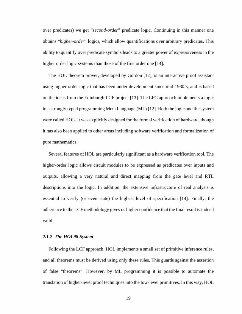
allows a hierarchal way of creating more complex theories as shown in Figure 2.1. By
proceeding this way, theories for new types can be created, e.g. floating-point theory, real
21
numbers theory, etc. New goals based on these types can be proved directly using the new-
proved libraries.
Figure 2.1: Hierarchy of Theories
In this work, we have used the HOL98 theorem prover, an adoption by Larsenet al.[27]
of HOL90 to the Moscow ML [12]. In addition to the usual programming language
expressions, ML has expressions that evaluate to terms, types, formulas, and theorems of
the HOL’s deductive apparatus [13]. The HOL system supports a natural deduction style
of proof, with driven rules formed fromeight primitiveinference rules. All inference rules
are implemented using ML functions, and their application is the only way to obtain
theorems in the system. Once proved theorems can be saved and used in future proofs. A
tactic in HOL98 is an ML function that is applied to a goal to reduce it to its subgoals, or
to simplify it. A tactical is a functional that combines tactics to form new tactics.
HOL98 is a powerful hardware verification system, on one hand, it derives its strength
from the expressiveness of higher-order-logic, it drives strength from the effectiveness of
the automated theorem proving facilities it provides. HOL can also capture the various
abstraction mechanisms and hierarchical descriptions, thereby making it very useful for
large designs, and also the logic itself can be extended to allow formalization of virtually
any mathematical theory.
Theory 1 Theory 2
Theory 3
Theory 5
Theory 4
22
2.2 Hardware Verification using HOL
2.2.1 Modeling Hardware Behavior using HOL
The essential step in any hardware verification task is the modeling of both the
implementation and specification of the system required to be verified. A significant
advantage of predicate logics are the ability to use functions and predicates to represent
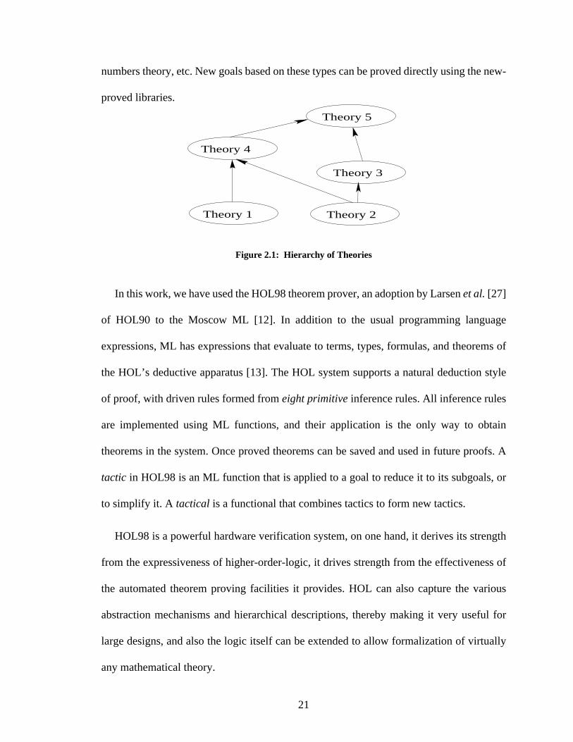
circuit models. Using new constants (refer to constant definition inSubsection 2.1.1),
predicates can be used to abbreviate complex circuit description. Using this mechanism, the
module in Figure 2.2 can be defined as:
Module (x1,x2...,y1,y2...)
Different logic relations can then be used inside this predicate to define the relation
between the inputs and outputs. For example in the lower level operators like AND or OR
operators can be used for describing these relations. In larger circuits, these operators will
not be enough, since the relation between different modules need to be described.
Figure 2.2: Circuit Module as a Black Box
A strong point of higher order logic is that constant definitions can still be used in such
a way that they reflect the composition of several modules. The predicates modeling the
behavior of the modules are conjunctively connected forming a new predicate, this was
........
X1
ModuleX
X
1
2
n
y
y
y
2
2

23
described as the hiding property [27]). Using this property, the formalization of a multi-
module as the one shown in Figure 2.3, will be modeled in HOL logic as:
M(x1,x2,x3,y1,y2) := ∃ sig1 sig2 . M1(x1,x2,sig1,y1) M2(sig1,x2,sig2)
M3(x3,sig2,y2)
Figure 2.3: Composition of Modules
The different intermediate signals can be considered as wires connecting different
modules. In Figure 2.3, the two signals,sig1andsig2, connect modules M1, M2, and M3.
The collection of these three modules build a new module M, which can be used as a higher
level representation of this system.
2.2.2 Performing Proofs using the HOL System
A proof in HOL is constructed by repeatedly applying inference rules to axioms or to
previously proved theorems. Since proofs may consist of large number of steps, it is
necessary to provide tools to make proof construction easier for the user. HOL supports two
styles of interactive proof: forward proof and backward proof styles.
∧ ∧
x
x M1
y
M2y
M3x
sig
sig
1
1
2
22
1
3
M

24
2.2.2.1 Forward Proofs in HOL
In the forward proof style, inference rules are applied in sequence to previously proved
theorems until the desired theorem is obtained [27]. The user specifies the rule to be applied
at each step of the proof, either interactively or by writing an ML program that calls the
appropriate sequence of procedures.
Forward proof is not the easiest way of doing proof, since the exact details of a proof are
rarely known in advance. It can work with small circuits and shallow mathematical proofs
but it would be considered unpractical for larger proofs. The forward proof style is
unnaturalandtoo ‘low level’ for many applications [2]. It suffers of two main handicaps
[12]:
1. It is usually quite hard to know where to start.
2. In general, there would be a lot of book keeping allocated with any large proof.
2.2.2.2 Backward Proofs in HOL
An important advance in proving using HOL was made by Robin Milner [13] in the
early 1970s when he invented thetactics, introducing a new proof methodology called the
Backward proof.
A tactic is a function that performs two things [12]:
1. Splits a ‘goal’ into ‘subgoals‘.
2. Keeps track of the reason why solving the subgoals will solve the goal. This is necessary
because all theorems in the system must ultimately be obtained by forward proof.
The idea behind a backward proof in HOL are that we recursively apply tactics to
decompose a goal into a tree of subgoals until all the leaves are simple enough to prove [2].
25
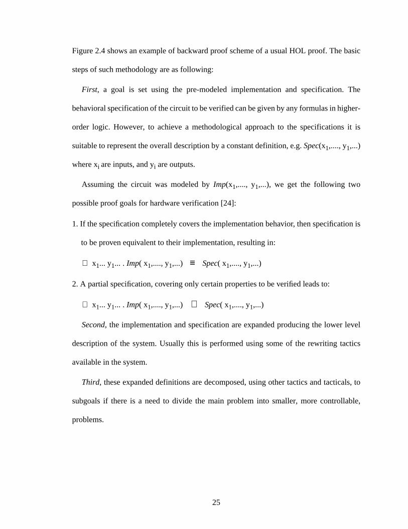
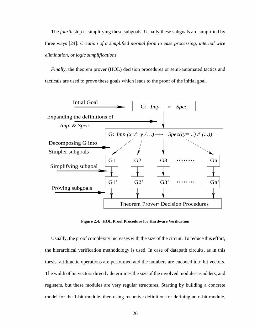
Figure 2.4 shows an example of backward proof scheme of a usual HOL proof. The basic
steps of such methodology are as following:
First, a goal is set using the pre-modeled implementation and specification. The
behavioral specification of the circuit to be verified can be given by any formulas in higher-
order logic. However, to achieve a methodological approach to the specifications it is
suitable to represent the overall description by a constant definition, e.g.Spec(x1,...., y1,...)
where xi are inputs, and yi are outputs.
Assuming the circuit was modeled byImp(x1,...., y1,...), we get the following two
possible proof goals for hardware verification [24]:
1. If the specification completely covers the implementation behavior, then specification is
to be proven equivalent to their implementation, resulting in:
x1... y1... . Imp( x1,...., y1,...) Spec( x1,...., y1,...)
2. A partial specification, covering only certain properties to be verified leads to:
x1... y1... . Imp( x1,...., y1,...) Spec( x1,...., y1,...)
Second, the implementation and specification are expanded producing the lower level
description of the system. Usually this is performed using some of the rewriting tactics
available in the system.
Third, these expanded definitions are decomposed, using other tactics and tacticals, to
subgoals if there is a need to divide the main problem into smaller, more controllable,
problems.
∀ ≡
∀ ⇒
26
The fourth step is simplifying these subgoals. Usually these subgoals are simplified by
three ways [24]:Creation of a simplified normal form to ease processing, internal wire
elimination,or logic simplifications.
Finally, the theorem prover (HOL) decision procedures or semi-automated tactics and
tacticals are used to prove these goals which leads to the proof of the initial goal.
Figure 2.4: HOL Proof Procedure for Hardware Verification
Usually, the proof complexity increases with the size of the circuit. To reduce this effort,
the hierarchical verification methodology is used. In case of datapath circuits, as in this
thesis, arithmetic operations are performed and the numbers are encoded into bit vectors.
The width of bit vectors directly determines the size of the involved modules as adders, and
registers, but these modules are very regular structures. Starting by building a concrete
model for the 1-bit module, then using recursive definition for defining an n-bit module,
G: Imp (x /\ y /\ ..) Spec((y= ..) /\ (...))
G1 G2 G3 Gn
G: Spec.Imp.
........
........G1’ G2’ G3’ Gn’
Theorem Prover/ Decision Procedures
Intial Goal
Simpler subgoals
Decomposing G into
Proving subgoals
Simplifying subgoal
Imp. & Spec.
Expanding the definitions of

27
HOL gives a very strong tool forgeneric circuit modeling and verification. These circuits
will be verified only once using mathematical induction procedure then this result can be
always generalized, used for any arbitrary bit width. The verification effort of these
modules is only done once then the result can always be reused directly. This dramatically
decreases the proof time in mathematical circuits. On the other hand, induction proofs
require a higher effort in finding suitable induction schemes, i.e., a higher degree of manual
interaction [24].

28
Chapter 3
Formal Modeling of the Exponential Function
3.1 Table-Driven Exponential Function (Mathematical Background)
Using an approximate polynomial expansion, Tang [40] has developed an algorithm for
computing the floating-point exponential function using what he calls a Table-Driven
approach. In this approach, the input is first reduced to a certain working precision where
r (will be discussed shortly) will be bounded by , whereL
is an integer larger than or equal to 1, chosen beforehand, (for instance,L = 4 for single
precision). Then this inputX is considered to be composed of:
wherem andj are integers, and r is a real number,|r| log 2/64
Starting from this equation, the exponential function can be constructed as follows [40]:
Theexponential of Xwill hence be equal to
2 2L 1+⁄log– 2 2L 1+⁄log,[ ]
X32 m j+×( ) 2log( )×
32----------------------------------------------------- r+=
<
X m 2log×( ) j 2log×( )32
------------------------ r+ +=
X( )exp m 2log×( ) j 2log×( )32
------------------------ r+ + exp=
2m
log( ) 2
j32------
log r+ +
exp=

29
Here, exp (r) can be represented using Taylor’s expansion as follows:
wherep(r) = exp (r) -1, anda1, a2,...are the coefficients of Taylor expansion.
Returning to the exponential function:
The main objective of the algorithm is isolatingmandj, and evaluating the approximating
polynomial. According to [40], four steps are needed to compute this exponential function:
Step 1:Filter any out-of-bounds inputs that occur. As mentioned before,X should be a
number between . So, ifx is NaN (not-a-number, invalid IEEE-754
format), out of range, zero, positive or negative infinity, the algorithm would either be able
to compute it by an approximated arithmetic operations (as in the case of positive or
negative infinity), or not able to solve it at all (as for NaN).
Step 2: Start the computation by first calculatingN,
whereINVL is a floating-point constant approximately equal to32/log 2 in our case, and
INTEGERis the default IEEE-754 round-to-nearest mode. ThisN is composed of two parts,
whereN1 = 32 * m, and N2 = j
The variablesm andj were derived, from the previous result as follows [40]:
2m 2 j 32/ r( )exp+ +=
p r( ) r a1 r×( ) a2 r2×( ) a3 r3×( ) …+ + + +=
x( )exp 2m 2j 32/ p r( ) 1+( )××=
2log( ) 32⁄– 2 32⁄log,[ ]
N INTEGER X INVL×( )=
N N1 N2+=
j N2=

30
With the value ofN, and considering r equal to r1 + r2, where r2 and r1 satisfy |r2| <<
|r1| so that r1+r2 represents r = X- (N * log 2 / 32)with a great accuracy.r1 andr2 can be
calculated as follows:
If then
else
and
L1 andL2 are constants, whereL1 + L2 approximateslog 2/32to a precision higher than
that of single precision (the working one).
Step 3:Compute the polynomialp(r), similar to the Taylor expansion, as follows [40]:
where the coefficients (a1anda2) are obtained from a Remez algorithm calculated by Tang
[40].
Step 4:The values of 2j/32, j= 0,1,....32, are calculated beforehand and represented by
two working-precision numbers (single precision in our case),SleadandStrail. Their sum
approximates to roughly double the working precision. Finallyexp(x)is calculated as
follows:
mN132-------=
N 29≥
r1 x N L1×–( )=
r1 x N1 L1×–( ) N2 L2×–=
r2 N L2×–=
r r1 r2+=
Q r r a1 r a2×+( )××=
p r( ) r1 r2 Q+( )+=
2 j 32/

31
3.2 Table Driven Exponential Function Specification
In this chapter, we will discuss the specification model we formalized for the table-
driven exponential function. As discussed in the previous chapter, the scope of this thesis
is to verify that the RTL hardware implementation of the exponential function conforms
with the behavioral description written in [15], shown in Figure 3.2.
As discussed above, we were faced by the flatness problem of the specification, which
was not directly useful for a hardware synthesis and/or verification. We have divided this
specification into six intermediate blocks (modules), where the conjunction of these blocks
(Figures 3.1, and 3.2) represents the RTL code described below. Trying to achieve
maximum modularity for the design, we have tried to minimize the interfaces between
different modules. This helps us to divide the verification tasks into well-defined smaller
ones. Each of these blocks was also divided into smaller specifications giving us smaller
sub-specifications clearly related to the goals needed to be proved.
The highest-level system specification in HOL is as follows:
S Strail j( ) Slead j( )+ 2 j 32/≈=
x( )exp 2m × Slead j( ) Strail j( ) S p r)( )×+( )+=
IEEE_EXP_SPEC X EXP = ∃ N N1 M R1 J R2 Strail Stail EXP_in P_R.
( M_J_SPEC X N N1 M J)( R1_R2_SPEC X N N1 J R1 R2)( Get_J_SPEC J Strail Stail)( P(R)_SPEC R1 R2 P_R)( EXP_CAL_SPEC Stail Strail M P_R EXP_in)( Compare_SPEC EXP_in X Out_EXP)
∧∧
∧∧
∧

32
Where the six main modules composing the system are:
m and j computing block(M_J_SPEC): responsible for half ofStep 2(cf. Section 3)
by computing the value ofm andj. Its input is the number X and its outputs are J, M, N,
and N1.
r1 and r2 block(R1_R2_SPEC): responsible for the second half ofStep 2, it computes the
values ofr1 andr2. Its inputs are X, N1, N2 (equal to J) and its outputs are the two floating-
point numbers R1 and R2.
p(r) block (P_R_SPEC): computes the value of p(r); it takes R1 and R2 and outputs P_R.
Slead and Strail block(Get_J_SPEC): a floating-point multiplexer module, where the
value of J decides which values for Strail and Slead should be chosen. Its input is just the
number J and its outputs are Slead and Strail.
Exponent calculation block(Exp_Cal_SPEC): the main computational block where
finally the exponential function is computed. It takes Slead, Strail, M and P_R as its inputs
and output is the EXP_X.
Checking block(Compare_SPEC): the compare and decision module. According to the
value of input X, this module decides whether to choose the computed value of the
exponent or another output as NAN (Not A Number). It takes X and the computed exponent
as its inputs and the final answer is the output (OUT_EXP_X).

33
Figure 3.1: The Modular Organization of Exponential Function Specification
There is a high level of regularity in these six modules where floating-point operations,
such as addition, and multiplication are the main sub-modules in all of them. This will help
us in the reuse of the developed models and theories in building the higher levels of the
specification. Each of the six modules was modeled as a conjunction of lower level
components. As an example, we will describe the m-and-j module specification
(M_J_SPEC).
X (Float)
J (Int)
R1 (Float)
M (Int)
EXP_X_SPEC
N (Int)
N1 (Int)
M_J_SPEC
R1_R2_SPEC P(R)_SPEC
Get_J_SPEC Exp_Cal_SPEC
Com
pare
_SPE
C
R2 (Float)
Slead (Float)
Strail (Float)
P(R) (Float)
EXP(X) (Float)

34
Figure 3.2: The Behavioral Specification for the Exponential Function in “while-language” [2]
Int_32 = Int(32)Int_2e9 = Int (2 EXP 9)Plus_one = float (0, 127, 0)THRESHOLD_1 = float (0, 134, 6066890)THRESHOLD_2 = float (0, 102, 0)Inv_L = float (0, 121, 3240448)L1 = float (0, 121, 3240448)L2 = float (0, 102, 4177550)A1 = float (0, 126, 68)A2 = float (0, 124, 2796268)
var x:float, E:float, R1:float, R2:float, R:float, P:float, Q:float,S:float, E1:float, N:Int, N1:Int, N2:Int, M:Int, J:Int;
if Isnan (X) then E:= Xelse if X == Plus_infinity then E:= Plus_infinityelse if X == Minus_infinity then E:= Plus_Zeroelse if (abs(x) > THRESHOLD_1 then Checking blockif X > Plus_Zero then E:= Plus_ infinityelse E:= Plus_Zeroelse if abs(X) < THRESHOLD_2 then E:= Plus_one + Xelse(
N:= INTRND (X * Inv_L);N2:= N% Int_32; m and j computing blockN1:= N - N2;M:= N1 / Int_32;J:= N2;
if abs (N) Int_2e9 thenR1:= (X-Tofloat(N1) * L1) - Tofloat (N2) * L1 r1 and r2 block else R1:= X - Tofloat(N) * L1;R2:= Tofloat(N) * L2;
R:= R1 + R2;Q:= R * R (A1 + R * A2); p(r) blockP:= R1 + (R2 + Q);
S:= S_Lead(J) + S_Trial(J); Slead and Strail block
E1:= S_Lead(J) + (S_Trial(J) + S * P); Exponent calculation blockE:= Scalb (E1, M);

35
Figure 3.3: Specification of the M-J Module (M_J_Spec)
The M_J_SPEC is responsible for computing themandj values mentioned before. It is
composed of the conjunction of five sub-specifications as shown in Figure 3.3. These sub-
specifications are the floating-point multiplication module (FP_MUL_SPEC), floating-
point to integer approximation module (FP_INT_SPEC), Modulo 32 module
(Mod_32_SPEC), floating-point subtraction module (FP_Sub_SPEC), and division by 32
module (Div_32_SPEC). Heremandj are integer valued numbers, even though they were
represented in the IEEE-754 floating-point format, since it is easier to use them afterwards
in this format. In short, this module would have one input (X) and a constant32/log 2,
composed of three parts (sign, exponent and mantissa) and four outputs (J, M, N, and N1),
each composed of the same three parts. This was modeled in HOL as follows:
X (Float) N2 (Int)
32/ log 2
N (Int)N1 (Int)
J (Int)
M (Int)
FP_MUL_SPEC Mod_32_SPECFP_to_INT_SPEC
Sub_SPEC Div_32_SPEC

36
Figure 3.4: Specifying the Floating-Point Multiplier
Each of these main modules is then hierarchically top-down specified to reach the full
specification of this system. As an example of the next levels specification, we consider the
floating-point multiplier sub-module (Figure 3.4). This sub-module has three datapaths: the
sign, the exponent and the mantissa. For the sign and the exponent, the specification could
be done directly on this level, but for the mantissa we have to build another level of
M_J_SPEC X N N1 M J =∃ const s1.
( valu const 31 = 132 * 2 EXP 23 + 3713595 )( FP_MUL_SPEC X const s1)( FP_to_INT_SPEC s1 N)( Mod_32_SPEC N J)( FP_Sub_SPEC N J N1)( DIV_32_SPEC N1 M)
∧∧
∧∧
∧
Subtract
Subtract
Subtract
Check For Count
XOR
M3 (23 bits)
e2 (8 bits)
e1 (8 bits)01111111
Add Add
0111111101111111
e3 (8 bits)
Exponent Module
1
1
M1 (23 bits)
M2 (23 bits)Multiply Shift Left (from 24 - 0)
Trancate
S1
S2
S3
Sign Module
Mantissa Module
Concatenate
Concatenate
check

37
hierarchical modules and give lower level specifications. This can be formalized as follows
using HOL:
Figure 3.5: distrib_Spec and collect_Specand their Usage in the Modeling Process
Wheredistrib_Specand collect_Spec(shown in Figure 3.5) are the specifications of
two main functions in floating-point implementation. Thedistrib_Specis responsible for
taking the floating-point number as a bit vector and distributes it to sign, exponent, and
mantissa. While thecollect_Specis performing the opposite taking the outputs and
returning the bit vector again. The specifications of both functions are as follows:
FP_MUL_SPEC A B MULout overFlow=∃ check A_m B_m A_e B_e A_s B_s.
(distrib_Spec A A_s A_e A_m) /\
( distrib_Spec B B_s B_e B_m) /\( Mantissa_SPEC A_m B_m MULout_m check)( Exp_SPEC A_e B_e MULout_e check overFlow)( Sign_SPEC A_s B_s MULout_s)( collect_Spec MULout_s MULout_e MULout_m MULout)
∧∧
∧
Disturub_Spec
.
.
.
.
.
.
.
.
Disturub_Spec
INPU
TS
Collect_Spec
Collect_Spec
Collect_Spec
OUTPUTS
Disturub_Spec
Floating-PointFunctions

38
This eases the modeling process as it decreases the signals transferred between the
modules to one bit vector per output instead of three. The multiplier Sign, Exponent and
Mantissa modules were specified as follows:
The latter code is composed of a number of sub-modules at the lower level. As an
example, we have shown the specification of one of the main modules which is the
multiplier:
distrib_Spec Input s e m =valu Input 31 = (bv s * 2 EXP 31)
+ ((valu e 7) * 2 EXP 23)+ (valu m 22)
collect_Spec s e m OUT=valu OUT 31 = (bv s * 2 EXP 31)
+ ((valu e 7) * 2 EXP 23)+ (valu m 22)
Sign_SPEC i1 i2 out = (out =((i1 = i2) => F | T))
EXP_SPEC e1 e2 e3 e4 overFlow =((valu e4 7 = (((( ((valu e1 7 - 127) + (valu e2 7 - 127))- valu e3 7)) + 127 < 2 EXP SUC 7)(((((valu e1 7 - 127)+(valu e2 7 - 127))-valu e3 7))+127)|((((((valu e1 7 - 127) + (valu e2 7 - 127)) - valu e3 7))+ 127) - 2 EXP SUC 7)))(overFlow = ~(((( ((valu e1 7 - 127) + (valu e2 7 - 127)- valu e3 7)) + 127 < 2 EXP SUC 7))))
Mantissa_SPEC A B MULout check =∃ A_1 B_1 MULout_pre MULout_pre_1 C P check1.
( Concatenate_SPEC 23 A A_1 T)( Concatenate_SPEC 23 B B_1 T)( MUL_SPEC 24 A_1 B_1 C P MULout_pre)( Check_SPEC MULout_pre check1 check)( Shifter_SPEC MULout_pre MULout_pre_1 check)( Truncate_SPEC MULout_pre_1 MULout 25)
⇒
∧
∧∧
∧∧
∧

39
Similarly, we would proceed to more and more sub-modules in order to describe the
circuit behavioral. We use intermediate sub-modules to change the very flat behavioral
level to a more hierarchical one to ease the verification task.
3.3 Implementation of IEEE-754 Exponential Function
In this section, we describe briefly the implemented VHDL code developed by Buiet al.
[1] of the IEEE-754 Exponential Function and its modular model in HOL. We were faced
with the same problem in the specification, which was the flatness of the design. The code
CELL_MUL_SPEC a b c p co po =(bv po = ((bv(a b)+bv c +bv p < 2) =>(bv(a b)+ bv c + bv p) |(bv (a b) + bv c + bv p) - 2))(co = ~ (bv (a b) + bv c + bv p < 2))‘--);
LEFT_SHIFT_SPEC X Y = ∀n. ((Y 0 = F) (Y (SUC n) = X n))
ROW_MUL_SPEC A b C P CO PO Aout= ∀ n.( ∃ c. (((bv (PO n) = ( bv ((A n) b) + bv (C n) +bv (P n) < 2 =>(bv ((A n) b) + bv (C n) + bv (P n))| (bv ((A n) b) + bv (C n) + bv (P n))- 2))((c n) = ~ (bv ((A n) b) + bv (C n)+ bv (P n)< 2))))LEFT_SHIFT_SPEC A AoutLEFT_SHIFT_SPEC c CO(C (SUC n) = F) (P (SUC n) = F))
(* Recursive definition of the Array module *)
( ARRAY_MUL_SPEC 0 A B C P Co Po Aout = ROW_MUL_SPEC A (B 0)C P Co Po Aout)( ARRAY_MUL_SPEC (SUC n) A B C P Co Po Aout = ∃ a p c.
ARRAY_MUL_spec n A B C P c p aROW_MUL_SPEC a (B (SUC n)) c p Co Po Aout)MUL_SPEC n A B C P MULout = ∃ Co Po Aout.ARRAY_MUL_SPEC n A B C P Co Po Aoutnadd_SPEC ((2*n)-1) Co Po F MULout (MULout (2 * n))
∧∧
∧∧
∧
∧
∧∧ ∧
∧∧
∧∧
∧
∧
∧
∧

40
was so flat it made it nearly impossible to be modeled, let alone verified. Thus, some design
changes had to be made, which involved keeping the same code properties but making the
design easier to model and verify. The main aim in the changes was to attack the following
criteria:
1) Logic Complexity:Hierarchical designs reduce the logic complexity in the circuit.
Also, in some modules the code could be changed to perform the same function, although
it is less complex.
2) Verification time and effort:it is very hard to model and verify a very large flat
design. Redesigning the VHDL code has saved a lot of time and effort needed in the
verification process. Also, this helped in emphasizing the modules needed to be verified,
i.e. clarifying the verification tasks needed for whole circuit verification.
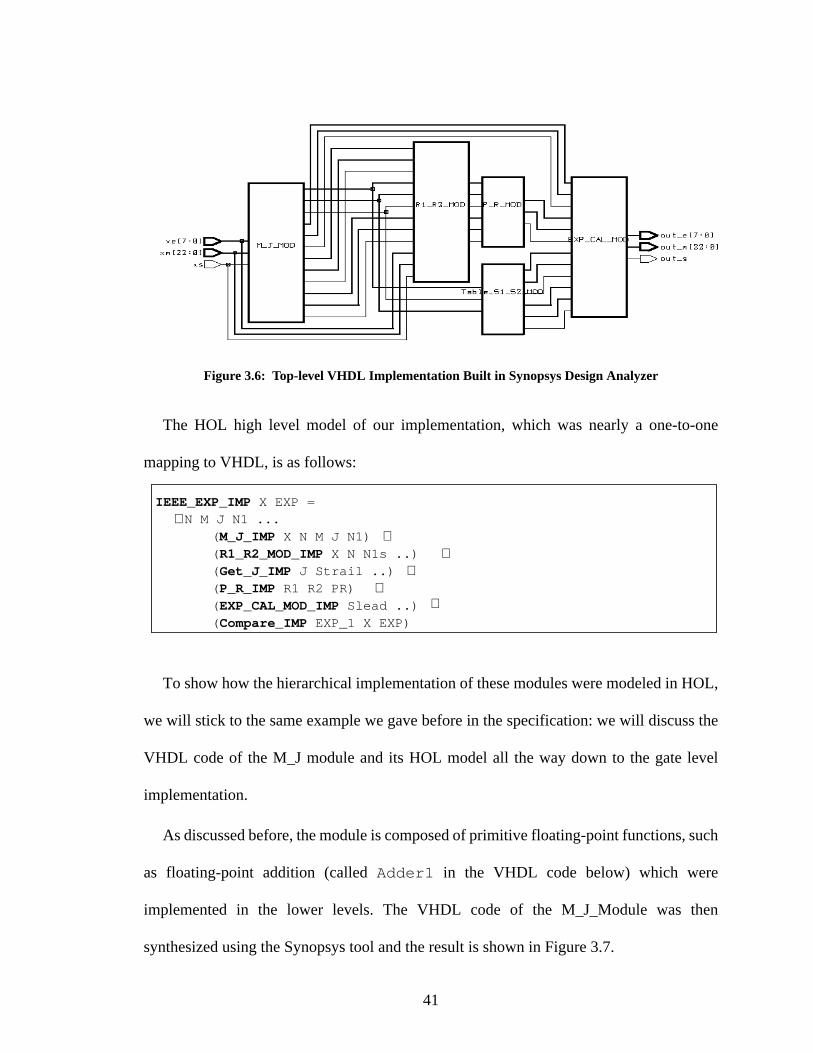
These goals were reached by deriving a modified VHDL implementation based on
modules from the code written in [1]. The new high-level RTL implementation is
composed of modules corresponding to the high level specification. We have shown in
Figure 3.6 the synthesis of this code as resulting from the Synopsys design analyzer tool
[39]. This figure only shows the exponential computation module.
41
Figure 3.6: Top-level VHDL Implementation Built in Synopsys Design Analyzer
The HOL high level model of our implementation, which was nearly a one-to-one
mapping to VHDL, is as follows:
To show how the hierarchical implementation of these modules were modeled in HOL,
we will stick to the same example we gave before in the specification: we will discuss the
VHDL code of the M_J module and its HOL model all the way down to the gate level
implementation.
As discussed before, the module is composed of primitive floating-point functions, such
as floating-point addition (calledAdder1 in the VHDL code below) which were
implemented in the lower levels. The VHDL code of the M_J_Module was then
synthesized using the Synopsys tool and the result is shown in Figure 3.7.
IEEE_EXP_IMP X EXP =∃ N M J N1 ...
( M_J_IMP X N M J N1)( R1_R2_MOD_IMP X N N1s ..)( Get_J_IMP J Strail ..)( P_R_IMP R1 R2 PR)( EXP_CAL_MOD_IMP Slead ..)( Compare_IMP EXP_1 X EXP)
∧∧
∧∧
∧

42
Figure 3.7: Synthesis of the M_J Module VHDL Implementation with Synopsys Design Analyzer
This code was directly modeled in HOL as follows:
Each of these main modules is then hierarchically top-down implemented to reach the
lower implementation of the system. For example, the floating-point multiplier
implementation, was implemented as in three sub-modules. These sub-modules were the
M_J_IMP X N N1 M J =∃ const s1.
( FP_MUL_IMP X const s1)( FP_to_INT_IMP s1 N)( Mod_32_IMP N J( FP_Sub_IMP N J N1)( DIV_32_IMP N1 M‘)
∧∧
∧∧

43
three usual paths of the floating-point numbers:sign, exponentandmantissa. The main
implementation was modeled as follows:
For the sign and the exponent, the implementation depends on other sub-modules as
XOR, and ADDER. This was modeled using following modules:
WherenSub_imp, andnAdd_impare the n-bit Subtractors and adder implementations,
respectively. The modeling of the mantissa is a little longer process, because the mantissa
FP_MUL_IMP A B MULout overFlow=∃ check A_m B_m A_e B_e A_s B_s.
( distrib_IMP A A_s A_e A_m) /\( distrib_IMP B B_s B_e B_m) /\( Mantissa_IMP A_m B_m MULout_m check)( Exp_IMP A_e B_e MULout_e check overFlow)( Sign_IMP A_s B_s MULout_s)( collect_IMP MULout_s MULout_e MULout_m MULout)
∧∧
∧
Sign_IMP i1 i2 out = XOR i1 i2 out
EXP_IMP e1 e2 e3 e4 overFlow =∃ s1 b bout1 s2 bout2 s3 bout3 s4 bout4 overFlow.
(valu b 7 = 127)(nSub_imp 7 e1 b F s1 bout1)(nSub_imp 7 e2 b F s2 bout2)(nAdd_imp 7 s1 s2 F s3 bout3)(nSub_imp 7 s3 e3 F s4 bout4)(nAdd_imp 7 s4 b F e4 overFlow)
∧
∧∧∧

44
got the main multiplication module. This was described in more than one level as shown
bellow:
The latter HOL description is composed of a number of sub-modules at the lower level.
To be consistent with the previous section, the integer multiplier implementation
(MUL_IMP) was implemented as follows:
Mantissa_IMP A B MULout check =∃ A_1 B_1 MULout_pre MULout_pre_1 C P check.
( Concatenate_IMP 23 A A_1 T)( Concatenate_IMP 23 B B_1 T)( MUL_IMP 24 A_1 B_1 C P MULout_pre)( Check_IMP MULout_pre check1 check)( Shifter_IMP MULout_pre MULout_pre_1 check)( Truncate_IMP MULout_pre_1 MULout 25)
∧∧
∧∧
∧
CELL_MUL_IMP a b c p co po =∃ s1. (and2 a b s1) (fa_imp s1 c p po co)
ROW_MUL_IMP A b C P CO PO Aout= ∃ c.(CELL_MUL (A (n)) b (C (n)) (P (n)) (c n) (PO (n))(ShiftLeFT_Imp n A Aout)(ShiftLeFT_Imp n c CO)(C (SUC n) = F)(P (SUC n) = F)
(* Recursive definition of the Array module *)
( ARRAY_MUL_IMP 0 A B C P Co Po Aout =ROW_MUL_IMP A (B 0) C P Co Po Aout)
( ARRAY_MUL_IMP (SUC n) A B C P Co Po Aout = ∃ a p c.ARRAY_MUL_IMP n A B C P c p aROW_MUL_IMP a (B (SUC n)) c p Co Po Aout)
MUL_IMP n A B C P MULout = ∃ Co Po Aout.ARRAY_MUL_IMP n A B C P Co Po Aoutnadd_imp ((2*n)-1) Co Po F MULout (MULout (2 * n))
∧
∧∧
∧∧
∧
∧
∧

45
For instance, the distribution module, which is responsible for taking the floating-point
number as a bit vector and distributing it to sign, exponent, and mantissa, was implemented
as follows:
Similarly, we would proceed to more and more sub-modules in order to reach the gate
level implementation. We use intermediate sub-modules to cover the gap between the RTL
and the gate level. This ends with simple gate building blocks of all the modules. These
gates are considered the elementary building blocks for the whole architecture. Examples
of these primitives are AND, OR, NOT, XOR, etc.
After fully modeling the specification and implementation of the system, the next task
was the verification process, which will be discussed in the next section along with the
experimental results. The high similarity between the implementation at high levels and the
specification considerably eased the verification task.
distrib_IMP Input s e m =(bv s = bv (Input 31) )(valu m 22 = valu Input 22)(e 0 = Input 23)(e 1 = Input 24) ...(e 7 = Input 30)
∧∧∧

46
Chapter 4
Verification of The Exponential Function Using
HOL
4.1 Verification Methodology
4.2.1 Verification and Hardware Design Path
A cornerstone of many of the CAD suites is the ability to design hierarchically [31]. In
a hierarchical design, the circuit entry stage is a process of designing parts. The entire
circuit is the top-level part in the hierarchy. It consist of a number of functional blocks, each
implemented as a part. These parts then in turn consist of lower level parts and so on. As
shown in Figure 4.1, the system designer manually derives the requirements of the system
as the system behavioral specification. This behavioral specification is then used to drive
an RTL design and usually this step is done manually with the help of some CAD tools
(e.g., Synopsys). By driving the RTL design, usually automatic tools are used to drive a
gate level then a final layout product is ready to be manufactured.
Figure 4.1: Design Stages and Errors [24]
Specification
Implementation
Architecture
Level
Implementation = Specification
Implementation = Specification
Implementation = Specification
RTL
Gate
Transistor
Layout
Faults

47
There is a large abstraction gap between specification and implementation. This gap
cannot be bridged in one move. Hence, a series of design (and verification) steps (levels)
are performed, reducing the abstraction levels until realizable description are available.
These levels, as mentioned by Kropf [24], areArchitecture (behavioral), Register-
Transfer, Gate, Transistor, andLayout levels (Figure 4.1). Table 4.1 shows the different
units and blocks used in each level.
Table 4.1 Abstraction Levels in Circuit Design [24]
In Table 4.1, different structures, behaviors, and data types are described. For instance,
the data types used in the design would differ from plain numbers (or real numbers), in the
highest levels of the design, to just pulses of different voltages indicating bits in the very
low levels.
Hierarchical design is important for two main reasons [31].First, it leads to a clear, well-
structured design. This facilitates “top-down” design and insures that any common element
is only entered once, simplifying both design and verification process.Second, it insures
the placement of related parts next to each other.
Level Behavior Structure Data Time
Architecture Algorithm Process Numbers Causality
RTL Data flow,FSM
Registers,ALU
Bit Vectors Clock cycles
Gate Booleanfunctions
Flip-flops,gates
buts discretedelaytime
Transistor Differentialequations
Capacitors,transistors
Voltage,current
Continuostime
Layout - area - -

48
In the design process, usually the implementation of a higher level is considered the
specification of the lower one as demonstrated in the Figure 4.1. Design faults may result
from erroneous transformation of the specification, given on a certain abstraction level, into
an implementation on the next lower level [24] (Figure 4.1). Three main fault classes can
be distinguished according to [24]. The first class encompassesdesign faults. The second
class resides inlocal optimizationsthat can be made in the same level. The third are
inherited implementation faults. As the late detection of design errors is largely responsible
for unexpected delays in realizing the hardware design, it is extremely important to ensure
correctness in each design step.
Formal verification methods have sometimes been accused of a lack of ability to get into
a whole industrial product design cycle. Factors like verification time, manpower, and
inability for handling large designs by verification tools were always showed to be the main
obstacle in using formal verification in industry. In this work, we have used HOL, a
theorem proving tool, along with the hierarchal and modular verification approaches to
insert formal verification into the whole design cycle of a floating-point circuit.
4.2.2 Exponential Function Verification
As shown in Figure 4.2, Harrison [15] formalized and verified that a behavioral
specification, an abstract algorithmic description he developed for the design, implies an
abstract mathematical description of the IEEE-754 Table-Driven Floating-Point
Exponential Function [37]. Starting form this behavioral specification, written in a “while-
language”, Bui et al. [1] developed an RTL implementation of the design in a previous part
in this project.

49
The goal of this work is using formal verification technique (using HOL tool) in the
modeling and verification of the latter implementation with respect to the behavioral
specification designed by [15]. We were also interested in the development of a formal
proof that the gate implementation, machine synthesized using Synopsys, implies the RTL
implementation.
Starting the modeling, it was noticed that the specification [15] is too flat for a lower
level modeling or verification. Therefore, a new modular behavioral specification was
introduced, where its modules are shown in Figure 3.1 with a corresponding source as
given in Figure 3.2. The same problem was faced in modeling the RTL implementation
where a newer modular VHDL code had to be driven from the older flat one. The new
modular implementation and specification were essentially considered to ease the
verification task, but it also put some guidelines for implementing testable circuit designs.
Figure 4.2: Verification Stages of the Exponential Function
Other Design ToolsHOL
HOL
HOL
HOL
HOL
Final Proof
1st Verifi. Task
2nd Verifi. Task
3rd Verifi. Task
Gate Level Imp.
HOL
Modular Beh. Spec.
Modular RTL Imp.
Provided
Logical
ImplicationSynthesized
Developedin this work
Machine
HierarchicalProof
Hand Modeled
while-language
Mathematics
VHDL
VHDL
VHDL
Gate Level Imp.
Modular RTL Imp.
Adopted in [3]
Flat RTL Imp. [3]
Algorithm Description [40]Algorithm Description [15]
Proved in [15]
Flat Behavioral Spec. [15]Flat Behavioral Spec.

50
After the modeling, the overall verification process is composed of four main tasks,
shown in Figure 4.2, where the left side of the figure shows the different verification stages
done by HOL, while the right side shows design stages, the different languages, and the
tools used in the design process:
First, we proved the correctness of the modular behavioral specification, the
specification we developed to meet the verification modular needs, against the main flat
specification provided in [15].
Second, we proved that the modular RTL implementation implies the modular
behavioral specification. Our new modular design implementation is the verified design
now which will be used afterwards to be both synthesized and verified in the next steps.
Third, we adopted aHierarchical Verification approach for the modeling and
verification of our design to prove that the synthesized gate level implementation implies
the modular RTL description. In this approach, the design is structured into a hierarchy of
components and sub-components, and specifications that describe “primitive components”
at one level of the hierarchy then become specifications of the intended behavior at the next
level down [5] (Figure 4.3).
Figure 4.3: Hierarchical Verification Approach
Spec.Imp.
Spec.Imp.
Spec.Imp.
Spec.Imp.
Spec.Imp.
Spec.Imp.
Spec.Imp.
Spec.Imp.
Spec.Imp.
Spec.Imp.
.......
Gate Level
RTL

51
Finally, The whole proof should be linked in one global proof covering the whole design
cycle of the floating-point exponential function. Starting from the gate level
implementation, we should be ending by the abstract mathematical description of the
function. These verification paths are shown in Figure 4.2, where the shaded boxes are the
material provided by [15], [37] and [1], while the white boxes represent those developed in
this work.
4.2 Formal Verification of the Exponential Function
The ultimate theorem to be proved should be:
Let X be the input and EXP the exponential output, then:
X EXP.
if THRESHOLD_2 THRESHOLD_1 then
EXP_GATE_IMP X EXP EXP_BEH_SPEC X EXP
The assumption on X is made by the boundary module within both the specification and
the implementation. So the goal would look as following in HOL:
∀ X EXP.
IEEE_EXP_GATE_IMP X EXP IEEE_EXP_BEH_SPEC X EXP
Where IEEE_EXP_GATE_IMPis the gate level implementation of the function and
IEEE_EXP_BEH_SPECis the behavioral implementation considered as our specifications.
This goal cannot be reached directly, due to the very high abstraction gap between the
gate and behavioral levels as described above. Therefore, the proof scheme was changed to
hierarchically prove that the gate level implies the more abstract RTL. Then this RTL was
∀
X≤ ≤
⇒
⇒

52
related, by a formal proof, to a modular behavioral specification. The latter was proved to
imply the high level flat behavioral specification. This can be formalized as follows in
HOL:
∀ X EXP.IEEE_EXP_GATE_IMP X EXP
IEEE_EXP_RTL_IMP X EXP (1)
∀ X EXP. IEEE_EXP_RTL_IMP X EXP
IEEE_EXP_MOD_BHV_SPEC X EXP (2)
∀ X EXP.IEEE_EXP_MOD_BHV_SPEC X EXP
IEEE_EXP_BHV_SPEC X EXP (3)
Where IEEE_EXP_RTL_IMPand IEEE_EXP_MOD_BHV_SPECare the RT and
modular behavioral specifications respectively.
Finally using equations (1), (2) and (3) we can reach the final goal stated again in
equation (4):
∀ X EXP.IEEE_EXP_GATE_IMP X EXP
IEEE_EXP_BHV_SPEC X EXP
Due to the high modularity of the two intermediate blocks, the goals (1), (2), and (3)
could be extended to sub-level modules’ specification and implementation, and then the
verification continues with these sub-level modules. These proofs were then composed to
yield the original goal. As an illustrative example, let’s consider the M_J module at the RT
level, whose specification and implementation have been shown above. In the following
theorem the goal was set as:
X N N1 M J.M_J_IMP X N N1 M J
⇒
⇒
⇒
⇒
∀

53
M_J_BEH_SPEC X N N1 M J
This was proven in HOL using the following tactic:
Theorems likeDIV_32_correct, Mod_32_correct, etc.are lemmas that were already
proved in previous verification steps. Usually in lower modules different strategies were
developed. For instance, induction (INDUCT_TAC) was mostly used in proving recursive
functions. Automatic tactics as PROVE_TAC and ARW_TAC were also used when the
goal was straightforward. These tactics take more machine time but they shorten the proof
and decrease the manpower needed.
Lower level implementations usually took more proof effort and time. As an example,
the verification goal of the floating-point multiplier, (cf. Sections 4.2, and 3.3) is set as
follows:
A B MULout OverFlow.
FP_MUL_IMP A B MULout overFlow
FP_MUL_SPEC A B MULout overFlow
This goal can be tackled by dividing it into smaller sub-goals, where every sub-goal
represents the verification of one of its sub-modules. For instance, for the main multiplier
block, ARRAY_MUL, this was done on many levels starting by verifying the cell, then the
⇒
REPEAT GEN_TAC THENREWRITE_TAC[M_J_Imp,M_J_SPEC] THENREPEAT STRIP_TAC THENEXISTS_TAC (--‘const_s:bool‘--) THEN..ARW_TAC[DIV_32_correct, Mod_32_correct , FP_to_INT_correct, FP_MUL_correct,FP_Sub_correct, FP_Add_correct ]
∀
⇒

54
row then the array multiplier. These proofs were held in theories (as all other HOL theories
proved), then they were in the higher levels of the hierarchy. For the cell, the row of the
main multiplier unit (array multiplier) (cf. Sections 4.2, and 3.3), the proof was as follows:
The correct theorems of the cell and row were used as lemmas in the higher level
verification. In this way, HOL is used to build a hierarchy of theorems which were used as
building blocks of other proofs afterwards. Proceeding in this way, the floating-point
multiplier verification was performed as follows:
Goal 1: a b c p co po. CELL_MUL a b c p co po
CELL_MUL_SPEC a b c p co po
Proof:REPEAT GEN_TAC THENREWRITE_TAC[CELL_MUL,CELL_MUL_SPEC] THENREWRITE_TAC[GSYM FA_CORRECT] THENREWRITE_TAC[fa_spec,and2] THENEXISTS_ELIM_TAC THENARW_TAC[]
Goal 2: n A b C P CO PO Aout. ROW_MUL_1 n A b C P CO PO Aout
ROW_MUL_SPEC_1 n A b C P CO PO Aout
Proof:REPEAT GEN_TAC THENREWRITE_TAC[ROW_MUL_1,ROW_MUL_SPEC_1] THENREWRITE_TAC[CELL_MUL] THENREWRITE_TAC[and2, GSYM FA_CORRECT] THENREWRITE_TAC[fa_spec]THENEXISTS_ELIM_TAC THENREPEAT STRIP_TAC THENEXISTS_TAC(--‘c:num->bool‘--) THENARW_TAC[ShiftLeFT_correct]
∀⇒
∀⇒

55
In HOL, we have the possibility of making use of previously proved theorems. This
saves a lot of time by eliminating the need for proving the same theory more than once. For
instance the above proof depends on other preproved theorems, so it looks really short,
although the goal is a real large one. This is clear in the usage of MUL_TRUE,
Concatenate_correct, Check_correct, and distrib_correct which were proved before.
Finally the goal for the distribution function (bothdistrib_impanddistrib_spec) will be
set and proved as follows using HOL:
Goal: A B MULout CHAN . FP_MUL_IMP A B MULout CHAN
FP_MUL_spec A B MULout CHAN
Proof:REPEAT GEN_TAC THENREWRITE_TAC[FP_MUL_IMP,FP_MUL_spec] THENREWRITE_TAC[Concatinate_IMP,Concatinate_SPEC] THENREPEAT STRIP_TAC THENEXISTS_TAC (--‘A_1:num->bool‘--) THENEXISTS_TAC (--‘B_1:num->bool‘--) THENEXISTS_TAC (--‘MULout_pre:num->bool‘--) THENEXISTS_TAC (--‘MULout_pre_1:num->bool‘--) THENEXISTS_TAC (--‘C:num->bool‘--) THENEXISTS_TAC (--‘P:num->bool‘--) THENEXISTS_TAC (--‘check:bool‘--) THENREWRITE_TAC[valu] THENASM_REWRITE_TAC[] THENUNDISCH_TAC (--‘MUL_imp 24 A_1 B_1 C P MULout_pre‘--) THENARW_TAC[MUL_TRUE,Concatenate_correct, Check_correct,Shifter_correct, Truncate_correct,distrib_correct, collect_correct]
∀⇒

56
In this proof, we have used some main tactics, such as different REWRITE_TAC forms,
to simplify the main goal, until the remaining part could be forwarded to an automatic
tactic, ARW_TAC, to solve it fully.
4.3 Experimental Results
A summary of the verification times for the whole system is given in Table 4.2. All the
experiments have been carried out on a Sun Ultra SPARC 2 workstation with 296 MHz
processor and 768 MB of memory. In the table, we have showed the verification times of
two main building blocks, the floating-point adder and multiplier. These modules took a
very high verification time, but due to the high reusability of pre-proven theorems and
lemmas, other building blocks and even the main module required much less verification
time. Also, it can be seen that the verification time for four of the six main modules are
Goal: Input s e m. distrib_IMP Input s e m
distrib_Spec Input s e m
Proof:REWRITE_TAC[distrib_IMP,distrib_Spec] THENONCE_REWRITE_TAC[MULT_SYM] THENREPEAT STRIP_TAC THENPURE_REWRITE_TAC[ num_CONV(--‘7‘--),... ,num_CONV(--‘1‘--)] THENREWRITE_TAC[valu,CONV_2] THENASM_REWRITE_TAC[] THENREWRITE_TAC[LEFT_ADD_DISTRIB] THENREWRITE_TAC[MULT_ASSOC] THENREWRITE_TAC[GSYM EXP_ADD] THENPURE_REWRITE_TAC[ num_CONV(--‘7‘--),...num_CONV(--‘1‘--)] THENREWRITE_TAC[ADD_CLAUSES] THENPURE_REWRITE_TAC[num_CONV(--‘31‘--),...num_CONV(--‘23‘--)] THENREWRITE_TAC[valu] THENARW_TAC[]
∀⇒

57
much smaller, since all these modules’ building blocks were pre-proved, it made the final
task shorter. The sum of the times of the systems showed here will be less than the total
verification time since there were some lemmas verified to achieve the final proof goal. The
whole code was composed of nearly 4600 lines.
Table 4.2 Verification Times of Different System Modules
Module Name CPU Time (in Sec.)
Floating-Point Addition 60.500
Floating-Point Multiplication 30.540
M_J Module 2.120
R1_R1 Module 5.620
P_R Module 3.420
EXP_Cal Module 1.970
IEEE_EXP Module 5.290
Total Verification Time 214.200

58
Chapter 5
Conclusions and Future Work
Most verification and testing tools will fail to verify a circuit with a deep datapath. The
IEEE-754 Table Driven Exponential function with its 32 bit input and 32 bit output
implementation is considered an impossible task for exhaustive simulation. For full
coverage with simulation we would have cases to be checked, which means that even
a 2 or 3 percent coverage would take very long simulation time. Another important aspect
is that in case of any detected error, the new code would need to be re-simulated fully to
make sure that this change did not affect any other module. Decision diagrams based formal
methods will, also fail to verify such circuits. Either because of the state space explosion
problem; or the lack of expressiveness of the specification languages, e.g. CTL properties
will fail to describe arithmetic operations.
In this thesis, formal verification methods, based on theorem proving techniques (HOL),
enabled a full sound verification of a complex floating-point algorithm. The higher-order
logic in HOL enabled the hierarchal and modular descriptions at different levels of
abstraction.
In this thesis, we have formalized and verified a hardware implementation of the IEEE-
754 Table-Driven floating-point exponential function algorithm using the HOL theorem
prover. The high ability of abstraction in the HOL verification system allows its use for the
verification task over the whole design path of the circuit, starting from the gate level
implementation of the circuit up to a higher level behavioral specification. To achieve this
goal, we have used both hierarchical and modular approaches for modeling and verifying
232

59
the floating-point exponential function in HOL, we did not find any errors in the RTL or
gate level implementation adopted.
Formal Verification, specially theorem proving, with some effort in automation and
training, can be integrated in the design cycle of mathematical circuits, increasing
confidence in these designs. The output of such effort leads to less design errors based on
the full coverage such techniques offer.
As a future work, this proof should be connected to the one developed by Harrison in
[15], to give a fully sound proof for such function starting from the gate level
implementation until the complete mathematical description of the function.
This project worked only onsingle precisionfloating-point numbers. It would be very
useful to extend this work to cover double and extended versions of the same standard.
Also, it would be interesting to specify and verify a generic version of the function which
can be directly used for any given precision.
Human efforts exerted in such a work is an interesting aspect to industry. In theorem
proving, it is very hard to define man-power used in the verification of each module,
because of the slow start of the process. However, time tends to diminish along the
verification path due to both an increase in the human knowledge of the system, and re-use
of previous tactics and theories. This process can be speeded up in a team work and through
the use of larger libraries of previous proofs.
On the other hand, more research is needed in the automation of both the modeling task
and the decision procedures of the HOL system. Tools used in modeling high definition
languages, VHDL and Verilog, or even subsets of them, in HOL language would decrease
significantly the need for human intervention and lead to the development of far more

60
accurate methods of implementation and specification modeling. HOL, as a system, needs
better documentation, as it is pretty hard to find tactics for non-HOL experts. A Graphical
User Interface would give HOL more capabilities to be used in industry.

61
Bibliography
[1] M. D. Aagaard, and C.-J. H Seger, “The formal verification of a pipelined double-pre-
cision IEEE floating-point multiplier”, Proc. ICCD’96, November 1995.
[2] G. Britwistle, S-K. Chin, and B. Garham, “new_theory ‘HOL’;;", An Introduction to
Hardware Verification in Higher Order Logic”, Computer Laboratory, Cambridge
University, UK, 1994.
[3] H. T. Bui, B. Khalaf, and S. Tahar, “Table-Driven Floating-Point Exponential Func-
tion”, CCECE’99, May 1999.
[4] R. S. Boyer, J. S. Moore. A Computational Logic Handbook. Academic Press, Boston,
1988.
[5] R.K. Brayton, et. al., “VIS; Proc. International Conference on Formal Methods in
Computer-Aided Design (FMCAD’96)”, Lecture Notes in Computer Science, Vol.
1166, Springer-Verlag, Palo Alto, CA., November 1996.
[6] Cadence, “Formal Verification Using Affirma FormalCheck: Manual”, V2.3, October
1999.
[7] V. A. Carreno, “Interpretation of IEEE-854 Floating-Point Standard and Definition in
the HOL system”, NASA Technical Memorandum 110189, September 1995.
[8] Y. Chen, and R. E. Bryant, “Verification of Floating-Point Adders”, Computer Science
Department, School of Computer Science, Carnegie Mellon University, 1998.
[9] Y. Chen, “Arithmetic Circuit Verification Based on Word-Level Decision Diagrams”,
School of Computer Science. Carnegie Mellon University, 1998.

62
[10]F. Corella, Z. Zhou, X. Song, M. Langevin, and E. Cerny, “Multiway Decision Graphs
for Automated Hardware Verification”, Formal Methods in System Design, Vol. 10,
February 1997.
[11]M. Cornea-Hasegan, “Proving the IEEE Correctness of Iterative Floating-Point Square
Root, Divide, and Remainder Algorithms”, Intel Technology Journal, 1998.
[12]M.J.C. Gordon and T.F.Melham, “Introduction to HOL: a theorem proving environ-
ment for higher order logic”, Cambridge University Press, 1993.
[13]M.J.C. Gordon, R. Milner and C. Wadsworth, “Edinburgh LCF: A Mechanized Logic
of Computation”.
[14]A. Gupta, “Formal Hardware Verification Methods: A Survey”, Formal Methods in
System Design, Kluwer Academic Publishers, 1992.
[15] J. R. Harrison, “Floating-point verification in HOL light: the exponential function”,
Technical Report number 428, University of Cambridge Computer Laboratory. UK,
June 1997.
[16] J. R. Harrison, “Theorem Proving with the real Numbers”, Technical Report number
408, University of Cambridge Computer Laboratory, December 1996.
[17] J. R. Harrison, “A Machine-Checked Theory of Floating-Point Arithmetic”, Proc.
TPHOLs’99, August 1999.
[18] J. R. Harrison, “Verifying the accuracy of polynomial approximations in HOL”,
TPHOLs’97, August 1997.
[19]D. Hoffmann, and T. Kropf, “Verification of a GF (2m) Multiplier-Circuit for Digital
Signal Processing”, Technical Report 22/98, University of Karlsruhe, 1998.

63
[20] Intel Inc., “Pentium Processors, Statistical Analysis of Floating-Point Flaw”, Intel
White Paper, Sec. 3, November 1994.
[21] Intel Inc., “Intel Architecture Software Developer’s Manual, Volume 2: Instruction Set
Reference”, Intel Corporation, 1997.
[22] IEEE Standards, “IEEE Standard for Binary Floating-Point Arithmetic Std. 754-
1985”, IEEE Standard, IEEE, 1985.
[23]C. Kern, and M. R. Greenstreat, “Formal verification in Hardware Design: A Survey”,
ACM transactions on Design Automation of Electronic Systems, Vol. 4 No. 2, April
1999.
[24]T. Kropf, “Introduction to Formal Hardware Verification”, Springer, 1999.
[25]M. Leeser, and J. O’ Leary, “Verification of a subtractive radix-2 square root algorithm
and implementation”, Proc. ICCD;95, October 1995.
[26]M.L. McMillan: Symbolic Model Checking.Norwell, MA: Kluwer, 1993.
[27]T. Melham, “Higher Order Logic and Hardware Verification”, Cambridge University
Press, 1993.
[28]T.F. Melham and M.J.C. Gordon, Higher Order Logic and Hardware Verification,
Cambridge Tracts in Theoretical Computer Science 31, Cambridge University Press,
1993.
[29]P. S. Miner, “Defining the IEEE-854 Floating-Point Standard in PVS”, NASA Tech-
nical Memorandum 110167, June 1995.
[30]P. S. Miner, and J. F. Leathrum, “Verification of IEEE Compliant Subtractive Division
Algorithms”, Proc. FMCAD’96, November 1996.

64
[31]P. Naish, P. Bishop, “Designing Asics”, Ellis Horwood Limited, 1988.
[32]M. Norrish, K. Slind, “A Thread of HOL Development”, University of Cambridge
Laboratory, July 2000.
[33]S. F. Oberman, “Division and Square Root for the AMD-K7 FPU”, Advanced Micro
Devices, 1997.
[34] J. O’Leary, X. Zhao, R. Gerth, and C. H. Seger, “Formally verifying IEEE Compliance
of Floating-Point Hardware”, Intel Technology Journal, 1999.
[35]B. Parhami, “Computer Arithmetic: Algorithms and Hardware Designs”, Oxford Uni-
versity Press, 2000.
[36]D. M. Russinoff, “A Mechanically Checked Proof of IEEE Compliance of a Register-
Transfer-Level Specification of the AMD-K7 Floating-Point Multiplication, Division,
and Square Root Instructions”, LMS Journal of Computation and Mathematics, De-
cember 1998.
[37]D. M. Russinoff, “A Mechanically Checked Proof of IEEE Compliance of the AMD
K5 Floating-Point Square Root Microcode”, Formal Methods in System Design, vol.
14, no. 1, January 1999.
[38] C.-J. Seger, “Voss- A formal hardware verification system user’s guide”, Tech. Rep.
93-45, Dept. of Computer Science, Univ. of British Colombia, 1993.
[39] Synopsis Inc., “Static Timing and Formal Verification: Online Manual”, Synopsis
Corporation, 2000.

65
[40]P. T. P. Tang, “Table-Driven Implementation of the Exponential Function in IEEE
Floating-Point Arithmetic”, ACM Transactions on Mathematical Software, vol. 15,
no. 2, 1989.