a high-order non-conforming finite element family - debreceni
TRANSCRIPT

A high-order non-conforming finite element family
doktori (PhD) ertekezes
Baran Agnes Eva
Debreceni Egyetem
Informatikai Kar
Debrecen, 2007

Ezen ertekezest a Debreceni Egyetem Matematika es Szamıtastudomanyok DoktoriIskola Valoszınusegelmelet, matematikai statisztika es alkalmazott matematika alprog-ramja kereteben keszıtettem a Debreceni Egyetem doktori (PhD) fokozatanak el-nyerese celjabol.
Debrecen, 2007. julius 2.
. . . . . . . . . . . . . . . . . . . . . . . . .Baran Agnes Eva
jelolt
Tanusıtom, hogy Baran Agnes Eva doktorjelolt 1998–2007 kozott a fent megnevezettDoktori Iskola Valoszınusegelmelet, matematikai statisztika es alkalmazott matemati-ka alprogramjanak kereteben iranyıtasommal vegezte munkajat. Az ertekezesbenfoglalt eredmenyekhez a jelolt onallo alkoto tevekenysegevel meghatarozoan hozzaja-rult. Az ertekezes elfogadasat javaslom.
Debrecen, 2007. julius 2.
. . . . . . . . . . . . . . . . . . . . . . . . .Dr. Stoyan Gisbert
temavezeto


Acknowledgement
Here I would like to thank all the people who have, either directly or indirectly,contributed to my dissertation.
First of all, to my husband, Sandor and my daughter, Zsuzsanna for their love, pa-tience and understanding.
To my parents for having brought me up and encouraging me.
To my supervisor, Dr. Gisbert Stoyan, who acquainted me with the beauty of nu-merical analysis and helped me in my proficiency with his instructions and usefuladvice.
To my friends and colleagues for their support on this long trip.
Koszonetnyilvanıtas
Itt szeretnek koszonetet mondani mindazoknak, akik direkt vagy indirekt modonhozzajarultak a disszertaciom elkeszıtesehez.
Eloszor is ferjemnek Sandornak es lanyomnak Zsuzsannanak, a szeretetukert, turel-mukert es megertesukert.
Szuleimnek, hogy felneveltek es batorıtottak.
Temavezetomnek, Dr. Stoyan Gisbertnek, aki megismertetett a numerikus analızisszepsegeivel, elorehaladasomat pedig utmutatasaval es hasznos tanacsaival segıtette.
Barataimnak es kollegaimnak, hogy tamogattak ezen a hosszu uton.

vi

Contents
Preface 1
1 Introduction and preliminary results 5
1.1 The Stokes equations . . . . . . . . . . . . . . . . . . . . . . . . . . . . 51.2 Saddle point problem and the inf-sup condition . . . . . . . . . . . . . 61.3 Variational formulation . . . . . . . . . . . . . . . . . . . . . . . . . . 71.4 Finite elements . . . . . . . . . . . . . . . . . . . . . . . . . . . . . . . 91.5 The discrete Stokes problem . . . . . . . . . . . . . . . . . . . . . . . . 121.6 Non-conforming approximations . . . . . . . . . . . . . . . . . . . . . . 141.7 Error estimates . . . . . . . . . . . . . . . . . . . . . . . . . . . . . . . 161.8 Crouzeix-Velte decomposition . . . . . . . . . . . . . . . . . . . . . . . 16
2 Some finite element families 19
2.1 Scott-Vogelius elements . . . . . . . . . . . . . . . . . . . . . . . . . . 192.1.1 Description and properties . . . . . . . . . . . . . . . . . . . . . 192.1.2 The nullspace of the discrete gradient . . . . . . . . . . . . . . 22
2.2 Fortin-Soulie element . . . . . . . . . . . . . . . . . . . . . . . . . . . . 362.3 Some higher order non-conforming finite elements . . . . . . . . . . . . 39
3 Gauss-Legendre elements 41
3.1 Definitions and properties . . . . . . . . . . . . . . . . . . . . . . . . . 413.2 The nullspace of the discrete gradient II . . . . . . . . . . . . . . . . . 523.3 The macroelement technique and the stability . . . . . . . . . . . . . . 553.4 Some remarks on the odd order elements . . . . . . . . . . . . . . . . . 59
4 Numerical results 63
4.1 Eigenvalues of the Schur complement operator . . . . . . . . . . . . . 634.2 Solution of a test problem . . . . . . . . . . . . . . . . . . . . . . . . . 66
Summary 69
Osszefoglalo 73
vii

viii CONTENTS
Bibliography 80
A List of Publications 85
B Conference talks 87

List of Figures
1.1 The nodal points for the standard Lagrangian basis on ∆0 if k = 4. . . . . . 10
2.1 Inner singular point. . . . . . . . . . . . . . . . . . . . . . . . . . . . . . 20
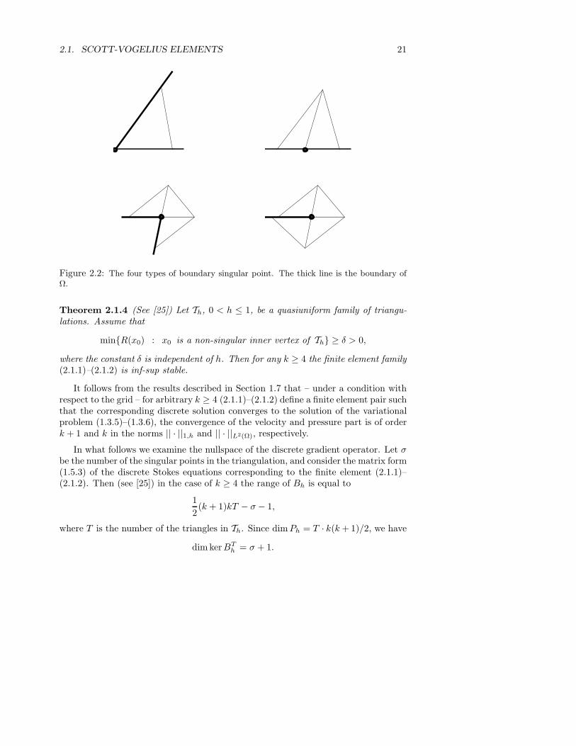
2.2 The four types of boundary singular point. The thick line is the boundary
of Ω. . . . . . . . . . . . . . . . . . . . . . . . . . . . . . . . . . . . . . 21
2.3 Criss-cross triangulation of the unit square in the case of n = 4 . . . . . . . 22
2.4 A triangulation with 208 nodes and 347 triangles. . . . . . . . . . . . . . . 23
2.5 A triangulation with 765 nodes and 1388 triangles. . . . . . . . . . . . . . 23
2.6 The reference triangular and a boundary singular point of type I. . . . . . . 25
2.7 A boundary singular point of type II. . . . . . . . . . . . . . . . . . . . . 26
2.8 The transformation B1 and B2 . . . . . . . . . . . . . . . . . . . . . . . 27
2.9 A boundary singular point of type III. and IV. . . . . . . . . . . . . . . . 29
2.10 An inner singular point. . . . . . . . . . . . . . . . . . . . . . . . . . . . 30
2.11 A domain Ω and a triangulation where NVh.2(Ω) ≥ N − 2 = 5 . . . . . . . . 33
2.12 Standard triangulation of the unit square in the case of n = 4 . . . . . . . 34
2.13 The function b∆ on the reference triangle. . . . . . . . . . . . . . . . . . . 37
3.1 A triangle and its three neighbours . . . . . . . . . . . . . . . . . . . . 42
3.2 The 4th-order non-conforming bubble function on the reference triangle. . . 50
4.1 Eigenvalues of Sh on the standard triangulation of the unit square, n=6.
Lower curve: P24−P3 (Scott-Vogelius element), here λ1 = λ2 = λ3 = 0, λ4 =
0.025975, upper curve: (P4 + B(4)n )2 − P3 (Gauss-Legendre element): λ2 =
0.056153. . . . . . . . . . . . . . . . . . . . . . . . . . . . . . . . . . . . 64
4.2 Eigenvalues of Sh on the criss-cross triangulation of the unit square, n=6.
Lower curve: P24 − P3 (Scott-Vogelius element), here λ1 = . . . = λ37 =
0, λ38 = 0.179739, upper curve: (P4+B(4)n )2−P3 (Gauss-Legendre element):
λ2 = 0.212876 . . . . . . . . . . . . . . . . . . . . . . . . . . . . . . . . 64
ix

x LIST OF FIGURES
4.3 Eigenvalues of Sh on the criss-cross triangulation of the unit square, n=6.
Lower curve: P22 − P1 (Scott-Vogelius element), here λ1 = . . . = λ37 =
0, λ38 = 0.1478315, upper curve: (P2 + B(2)n )2 − P1 (Gauss-Legendre ele-
ment): λ2 = 0.2414476 . . . . . . . . . . . . . . . . . . . . . . . . . . . . 654.4 Eigenvalues of Sh in the case of first order Crouzeix-Raviart element. . . . . 66
List of Notations
B(k)c,∆ kth-order conforming bubble function defined over a triangle ∆
B(k)n,∆ kth-order non-conforming bubble function defined over a triangle ∆
C∞(Ω) space of infinitely differentiable functions over ΩC∞
0 (Ω) space of infinitely differentiable functions having a compact support in Ω∆ Laplace operator∆ a triangle∆0 the reference trianglediam diameterdiv the divergence operatorΓ = ∂(Ω) the boundary of Ωgrad the gradient operatorh the discretization parameterH1
0 (Ω) the Sobolev space of functions with square integrable gradient and zeroboundary values (in the sense of traces)
H1(Ω) the Sobolev space of functions with square integrable gradientL2(Ω) space of square integrable functions over ΩL2
0(Ω) space of square integrable functions with zero integral over ΩLk the kth-order Legendre polynomial defined on the interval [0, 1]λi barycentric coordinates, i = 1, 2, 3Ω a domain in R
2
Ph the discrete pressure space
P(α,β)k the kth-order Jacobi polynomial on the interval [−1, 1] with parameters
(α, β) and leading coefficient 1.Pk the space of the polynomials with maximal degree kR the set of the real numbersrot the rotation operatorTh a triangulation of ΩVh the discrete velocity space
xi

xii LIST OF NOTATIONS
Preface
Numerous numerical experiments show that the use of high-order finite elements isadvantageous in solving flow problems [16], [22]. It is well known that the motionof an incompressible viscous fluid can be described by the Stokes equations. In thepresent dissertation we will consider triangular finite elements for the two-dimensionalStokes problem.
An example of a finite element family that is defined for arbitrary order are theTaylor-Hood finite elements where the velocity and the pressure are approximatedtrianglewise by polynomials of order k and k − 1, respectively, and the polynomialsare assumed to be continuous on the common sides of two adjacent triangles. Theelement is inf-sup stable [5].
In the case of the pressure it is common to use discontinuous approximations toensure the elementwise mass conservation property.
In [25] Scott and Vogelius investigated the Pk/Pk−1 finite element pair (polynomi-als of order k for the velocity and (k−1) for the pressure) where there is no continuityrequirement for the discrete pressures. The element is inf-sup stable for k ≥ 4 if thetriangulation does not contain near-singular points, i.e. points which are close to thesituation where the edges meeting in this point lie on two straight lines.
An other problem caused by the singular points is that in the presence of thesepoints the nullspace of the discrete gradient operator is larger than the nullspace of thegradient operator in the original problem (where it contains only constant functions).This means that while in the continuous case the pressure can be determined uniquelyup to an additive constant, after the finite element discretization of the problem wehave a system of linear equations which has a higher dimensional nullspace.
To ensure the grid independent stability one may consider the non-conformingelements. In [11] Crouzeix and Raviart defined a first-order non-conforming finiteelement pair, the second-, and third-order elements were described by Fortin andSoulie [13], and by Crouzeix and Falk [10], respectively. In all the three cases thekth-order (k = 1, 2, 3) polynomials which approximate the velocity are continuous onthe common side of two neighboring triangles only in the kth-order Gauss-Legendrepoints. These points are the roots of the kth-order Legendre polynomial definedover the given side of the triangle. In [11] the authors showed that the continuity
1

2 PREFACE
requirements in these points ensure the optimal order of convergence.
The construction of the second-order element differs from the cases k = 1, 3. Ifk = 1 or k = 3 then for the degrees of freedom one can choose the 3k Gauss-Legendre
points on the sides of the triangle and (k−2)(k−1)2 points distributed uniformly inside
the triangle.
If k = 2 then there exists a second-order polynomial which disappears in all thesix second-order Gauss-Legendre points on the sides of any triangle. This polynomialis called a second-order non-conforming bubble function. In this case one gets thevelocity part of the finite element by adding trianglewise the bubble function to thevelocity space of the second-order Scott-Vogelius elements.
In the past few years several authors have dealt with the study of non-conformingfinite elements.
In [7] the elements of order k = 4 and k = 6 are investigated. Similarly tothe second-order case the authors define bubble functions of order k and the non-conforming elements are given by enriching the corresponding conforming velocityspaces by these bubbles.
In [18] a non-conforming finite element family is described that is defined forarbitrary order. The authors also use bubble functions, but the construction differsfrom the earlier one: here a polynomial of order k + 1 is added trianglewise to thekth-order velocity space.
In the present work we deal with the description of a non-conforming finite elementfamily which generalizes the low-order (k = 1, 2, 3) cases. The family is defined forarbitrary order and for even k it is inf-sup stable without a restriction on the grid.We show that for even k the non-conforming bubble removes from the kernel of thediscrete gradient the non-constant pressures arising for the Scott-Vogelius elements ifsingular points are present.
This dissertation consists of four chapters. In Chapter 1 we give a short review ofthe basic notions and theorems about the finite element methods.
Since in the even order cases we will define the non-conforming element basedon the conforming Scott-Vogelius elements in Chapter 2 we examine the algebraicproperties of this family.
In Section 2.1.2 we investigate the nullspace of the discrete gradient operator whenthe triangulation contains singular points. Using the result about its dimension [25]we give a basis of this nullspace. Here we use orthogonal polynomials defined overtriangles [17].
In Section 2.2 we study the second-order non-conforming element defined by Fortinand Soulie - for even k we will construct the new non-conforming finite element family(called Gauss-Legendre elements) similarly to this case.
In Section 2.3 we shortly describe the fourth-, and sixth-order elements defined byY.Cha, M. Lee and S. Lee [7].
The detailed examination of the Gauss-Legendre elements is given in Chapter 3.In Section 3.1 we define the elements: velocity and pressure are approximated trian-
PREFACE 3
glewise by polynomials of order k and k − 1, respectively, and the discrete velocitiesare continuous on the common side of two neighboring triangles in the kth-orderGauss-Legendre points. For odd k we specify suitable degrees of freedom for the ve-locity part, and connected with the interpolation problem arising here we determinea general formula for the even-order non-conforming bubble function. For k = 2 thisgives the bubble used in [13] and for k = 4, 6, apart from a conforming part, thebubbles defined in [7].
In Section 3.2 we show that in the case of Gauss-Legendre elements for even k thenullspace of the discrete gradient operator is one-dimensional: it consists of constantfunctions. Here we use the results of Section 2.1.2 and we prove that by addingtrianglewise the non-conforming bubble function to the conforming velocity space thenullspace described in Section 2.1.2 becomes one-dimensional.
For even k the proof of stability is based on the macroelement technique whichwas described for the conforming cases by Stenberg [26]. In Section 3.3 a slightmodification of this method for the non-conforming case is given. For the proof weneed the result of Section 3.2 about the kernel of the discrete gradient.
The non-conforming bubble function has an important role in the stability. How-ever, for odd k there does not exist a kth-order polynomial defined over a trianglewhich disappears on the sides of the triangle only in the kth-order Gauss-Legendrepoints. In Section 3.1 we have described functions that can be considered as non-conforming bubbles over two adjacent triangles: they are equal to zero in the Gauss-Legendre points on the boundary sides of the quadrilateral formed by the triangles.In Section 3.4 we investigate whether the proof of stability given in the even ordercases can be modified using these bubbles.
In Chapter 4 we present some numerical results using Matlab computations. Fordifferent values of k and for various triangulations in the case of Scott-Vogelius andGauss-Legendre elements we give the value of the discrete inf-sup stability constantand we solve a test problem using fourth-order Gauss-Legendre elements.

4 PREFACE

Chapter 1
Introduction and preliminary
results
In the present chapter we introduce the basic notions and propositions that are neededin the presentation of the results of the author. Most of the definitions and theoremspresented here can be found in the monographs of Atkinson and Han [1], Braess [3],Brezzi and Fortin [6] and Ciarlet [8]. Besides this we provide a wide overview of thehistorical background of this research.
1.1 The Stokes equations
In the present work we will deal with the finite element solution of the two-dimensionalStokes equations. These equations describe the motion of an incompressible viscousfluid in a 2-dimensional domain. Let Ω ⊂ R
2 be a bounded domain with a Lipschitzcontinuous boundary. The Stokes problem is the following: find ~u : Ω → R
2 andp : Ω → R such that
−~∆~u + gradp = ~f, (1.1.1)
−div ~u = 0, (1.1.2)
~u|Γ = ~u0, (1.1.3)
where Γ = ∂Ω is the boundary of the domain, and ~f is a given external force field.Here ~u = (u1, u2)
T is the velocity vector and p is the pressure.Applying Green’s formula we obtain that for the solvability of the equations we
must have∫
Γ
~u0~n ds =
∫
Ω
div ~u dxdy = 0,
where ~n is the outward-pointing normal unit vector to Γ.
5
6 CHAPTER 1. INTRODUCTION AND PRELIMINARY RESULTS
In (1.1.1)–(1.1.3) the pressure is determined only up to an additive constant, but
for a fixed p the velocity vector is uniquely given, since the operator ~∆ is positivedefinite.
A solution ~u and p of (1.1.1)–(1.1.3) is called a classical solution if ~u ∈ (C2(Ω) ∩C(Ω))2 and p ∈ C1(Ω).
1.2 Saddle point problem and the inf-sup condition
Before formulating the weak version of the Stokes equations let us consider the solv-ability conditions of a saddle point problem. Let V and M be two Hilbert spaces withthe norms || · ||V and || · ||M , respectively, and let a : V × V → R, b : V × M → R becontinuous bilinear functionals,
|a(u, v)| ≤ Ma||u||V ||v||V , |b(u, q)| ≤ Mb||u||V ||q||M .
Suppose that f ∈ V ′ and g ∈ M ′, where V ′ and M ′ are the dual spaces of V and M ,respectively. Consider the following saddle point problem: find (u, p) ∈ V × M suchthat
a(u, v)+b(v, p) = 〈f, v〉 ∀v ∈ V, (1.2.1)
b(u, q) = 〈g, q〉 ∀q ∈ M. (1.2.2)
Theorem 1.2.1 (Brezzi’s theorem) Suppose that the bilinear forms a and b are con-tinuous and let
L : V × M → V ′ × M ′
(u, p) 7→ (f, g)
be the linear mapping defined by (1.2.1)–(1.2.2). Then L is an isomorphism if andonly if
1. for the bilinear form a with some α > 0
a(v, v) ≥ α||v||2V
holds for all v ∈ V0 := v ∈ V : b(v, q) = 0 ∀q ∈ M (that means a isV0-elliptic), and
2. there exists a constant β such that
infp∈M
supv∈V
b(v, p)
||v||V · ||p||M≥ β > 0 (1.2.3)
holds.
1.3. VARIATIONAL FORMULATION 7
Moreover, if the conditions above are satisfied then the solution of the problem (1.2.1)–(1.2.2) is stable in the sense
||u||V ≤||f ||
α+
(
a +Ma
α
)
||g||
β,
||p||M ≤
(
a +Ma
α
)
1
β
(
||f || +Ma
β||g||
)
.
The inequality (1.2.3) is called inf-sup condition.
1.3 Variational formulation
In this section we give the weak formulation of the problem (1.1.1)–(1.1.3) which is astarting point to get the finite element solution of the Stokes equations.
Let C∞(Ω) denote the space of infinitely differentiable functions, and let C∞0 (Ω)
be the subspace of C∞(Ω) which consists of functions having a compact support inΩ. In order to ensure the uniqueness of the solution p we will assume that
∫
Ω
p dx = 0,
and we define the space L20(Ω) in the usual way:
L20(Ω) :=
q ∈ L2(Ω) :
∫
Ω
q dx = 0
.
LetHm(Ω) :=
u ∈ L2(Ω) : Dαu ∈ L2(Ω), ∀ |α| ≤ m
be the Sobolev space of functions which have square integrable αth weak derivativesfor all |α| ≤ m. Denote by (·, ·)0 the usually inner product in L2. The space Hm(Ω)is a Hilbert space with the inner product
(u, v)m :=∑
|α|≤m
(Dαu, Dαv)0.
The corresponding norm is
||u||m :=
√
∑
|α|≤m
||Dαu||2L2(Ω), (1.3.1)
and the function
|u|m :=
√
∑
|α|=m
||Dαu||2L2(Ω) (1.3.2)
8 CHAPTER 1. INTRODUCTION AND PRELIMINARY RESULTS
defines a semi-norm on Hm(Ω).
First we will deal with the equations (1.1.1)–(1.1.3) in the case of homogeneousboundary conditions that is when ~u0 ≡ 0.
Denote by Hm0 (Ω) the completion of C∞
0 (Ω) with respect to the Sobolev norm|| · ||m. If Ω is bounded, then | · |m is a norm on Hm
0 (Ω) which is equivalent to || · ||m(see [3, Ch. II. §1.]).
Multiplying (1.1.1) with a test-function ~v ∈ (H10 (Ω))2 and integrating over Ω, from
the Green-formula we obtain
∫
Ω
grad~u : grad~v dx −
∫
Ω
p div~v dx = (~f,~v)0,
where
grad~u : grad~v :=
2∑
i=1
2∑
j=1
∂ui
∂xj
∂vi
∂xj,
(~f,~v)0 :=
∫
Ω
(f1v1 + f2v2) dx.
Similarly, from (1.1.2) with a test-function q ∈ L20(Ω) we have
−
∫
Ω
q div ~udx = 0.
Denote by a(·, ·) and b(·, ·) the following bilinear functionals:
a(~u,~v) :=
∫
Ω
grad~u : grad~v dx, (1.3.3)
b(~v, p) := −
∫
Ω
p div~v dx. (1.3.4)
Using these notations in the case of homogeneous boundary conditions the variationalformulation of the equations (1.1.1)–(1.1.3) is the following: find ~u ∈ (H1
0 (Ω)2 andp ∈ L2
0(Ω) such that
a(~u,~v)+b(~v, p) = (~f,~v)0 ∀~v ∈ (H10 (Ω))2, (1.3.5)
b(~u, q) = 0 ∀q ∈ L20(Ω). (1.3.6)
It can be shown (see e.g. [3, Ch. III, §5.]) that if for a solution (~u, p) of (1.3.5)–(1.3.6)~u ∈ (C2(Ω)∩C0(Ω))2 and p ∈ C1(Ω) hold, then (~u, p) is a solution of (1.1.1)–(1.1.3).
To prove the existence and uniqueness of the solution of (1.3.5)–(1.3.6), we willuse the Necas theorem [20]:
1.4. FINITE ELEMENTS 9
Theorem 1.3.1 Let Ω be a domain with Lipschitz continuous boundary. For allq ∈ L2
0(Ω) there exists a ~u ∈ (H10 (Ω))2 such that
q = div ~u and |~u|1 ≤ c0||q||L2(Ω) (1.3.7)
hold, and the constant c0 is independent of q and ~u.
Theorem 1.3.2 If Ω is a domain with Lipschitz continuous boundary then the vari-ational problem (1.3.5)–(1.3.6) has a unique solution.
Proof. We have to check the conditions of Theorem 1.2.1. The bilinear forms a and bare continuous and since |~u|1 = a(~u, ~u)1/2 is a norm on (H1
0 (Ω))2, the bilinear form ais elliptic on (H1
0 (Ω))2. To verify the inf-sup condition let q ∈ L20(Ω) be an arbitrary
function and let ~u ∈ (H10 (Ω))2 be a function for which (1.3.7) holds. Then the inf-sup
inequality follows from
b(−~u, q) =
∫
Ω
q2 dx = ||q||2L2(Ω) ≥1
c0||q||L2(Ω) · |~u|1.
2
1.4 Finite elements
Let Ω ⊂ R2 be a polygonal domain. We divide Ω into finitely many subdomains and
we will approximate the solution of the variational problem with functions which arepolynomials on each subdomain.
Definition 1.4.1 Let Th = ∆i, i = 1, . . . , n be a partition of Ω into triangles,where diam∆i ≤ h for all i = 1, . . . , n. We call Th a triangulation of Ω if thefollowing conditions are satisfied
1. Ω =⋃n
i=1 ∆i,
2. if i 6= j and ∆i ∩ ∆j 6= ∅ then exactly one of the following two conditions issatisfied
a. ∆i ∩ ∆j consists of exactly one point, and this point is a common vertexof ∆i and ∆j,
b. ∆i ∩ ∆j is a common edge of ∆i and ∆j .
Definition 1.4.2 (See [3]) A finite element is a triple (T, ΠT ,∑
T ) with the followingproperties:
1. T is a polyhedron in R2,
10 CHAPTER 1. INTRODUCTION AND PRELIMINARY RESULTS
2. ΠT is a subspace of C(T ) with finite dimension s,
3.∑
T is a set of s linearly independent functionals on ΠT . Each p ∈ ΠT isuniquely defined by the values of the s functionals in
∑
T . Since the functionalsusually involve point evaluation of a function or of its derivatives at points inT , we call these functionals interpolation conditions.
Remark 1.4.3 Usually the set ΠT itself is called a finite element.
Definition 1.4.4 If there is a set of points which uniquely determines any functionin the finite element space by its values at the given points, these points are callednodal points and the functionals that map the nodal points on the function values arecalled (Lagrange type) degrees of freedom.
Remark 1.4.5 In Definition 1.4.2 polyhedrons could be both triangles and quadri-laterals. However, in the present work we use only triangular finite elements.
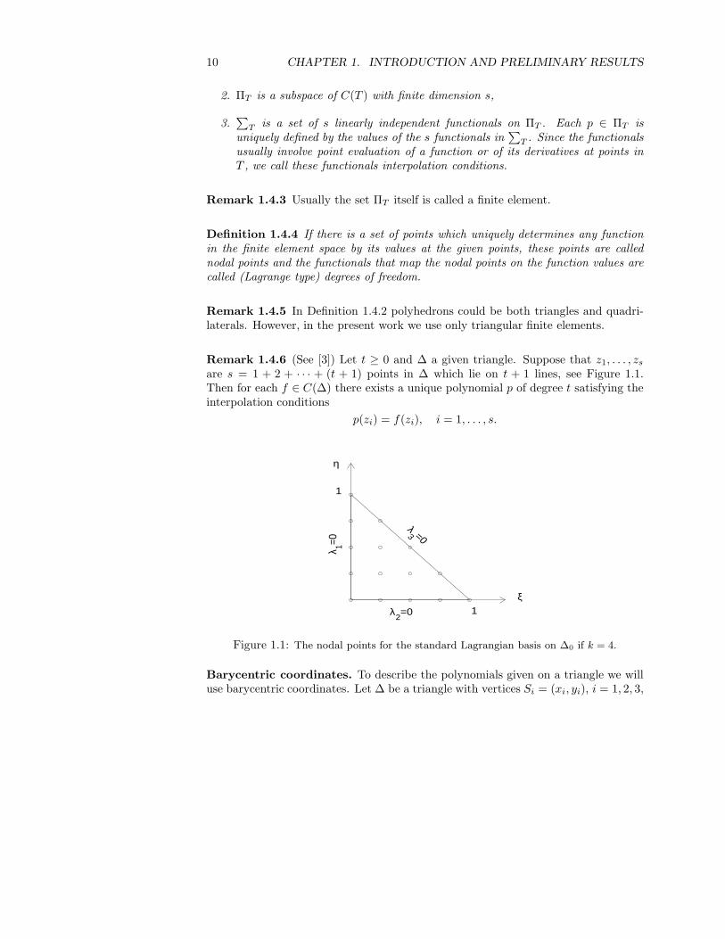
Remark 1.4.6 (See [3]) Let t ≥ 0 and ∆ a given triangle. Suppose that z1, . . . , zs
are s = 1 + 2 + · · · + (t + 1) points in ∆ which lie on t + 1 lines, see Figure 1.1.Then for each f ∈ C(∆) there exists a unique polynomial p of degree t satisfying theinterpolation conditions
p(zi) = f(zi), i = 1, . . . , s.
λ 1=0
λ2=0
λ3 =0
ξ
η
1
1
Figure 1.1: The nodal points for the standard Lagrangian basis on ∆0 if k = 4.
Barycentric coordinates. To describe the polynomials given on a triangle we willuse barycentric coordinates. Let ∆ be a triangle with vertices Si = (xi, yi), i = 1, 2, 3,

1.4. FINITE ELEMENTS 11
and let P = (x, y) be a point in ∆. If for λ1, λ2, λ3
x1 x2 x3
y1 y2 y3
1 1 1
λ1
λ2
λ3
=
xy1
(1.4.1)
holds, then we call λ1, λ2, λ3 the barycentric coordinates of P in ∆. The determinantof the matrix in (1.4.1) is equal to 2|∆|, where
|∆| =1
2(x1y2 − y1x2 + x2y3 − y2x3 + x3y1 − y3x1)
is the area of the triangle ∆. Thus λ1, λ2, λ3 are simply the ratios of the areas oftriangles S2S3P , S1S3P and S1S2P , respectively, to |∆|.
The following lemma will be useful if we want to calculate integrals of polynomialsover the triangle ∆ (see [15]).
Lemma 1.4.7 Let ∆ ∈ Th be an arbitrary triangle and denote by λ1, λ2, λ3 thebarycentric coordinates in ∆. In this case
∫
∆
λk1λℓ
2λm3 dx dy = 2|∆|
k!ℓ!m!
(k + ℓ + m + 2)!.
Denote by Pk(∆) the space of polynomials given on ∆ with maximal degree k.In what follows we will need the standard Lagrangian basis of Pk(∆), where ∆ ∈
Th. Consider the points γ(k)i , i = 1, . . . (k + 1)(k + 2)/2, in ∆ with the barycentric
coordinates (see Figure 1.1)
λ1 =j
k, λ2 =
ℓ
k, j = 0, . . . , k, ℓ = 0, . . . , k − j.
Then ui ∈ Pk(∆), i = 1, . . . , (k + 1)(k + 2)/2 is the standard Lagrangian basis ofPk(∆), if
ui(γ(k)j ) =
1, if i = j,
0, if i 6= j
holds for all i, j = 1, . . . , (k + 1)(k + 2)/2.
Remark 1.4.8 Let Th be a triangulation of the polygonal domain Ω. Consider oneach triangle the nodal points corresponding to the standard Lagrangian basis oforder k. In this case there are (k + 1) points on the edges of the triangles and therestriction of an arbitrary polynomial of order k to an edge is uniquely determinedby its values at these points. This means that if f : Ω → R is a function for whichf |∆ ∈ Pk(∆) holds for all ∆ ∈ Th, and f is continuous on the common side of twoadjacent triangles in these nodal points then f is globally continuous on Ω.
12 CHAPTER 1. INTRODUCTION AND PRELIMINARY RESULTS
Definition 1.4.9 (See [3]) Let Th be a triangulation of Ω, and let Vh be a family offinite elements for the partition Th. This family is called affine family if there existsa reference element (∆0, Π0,
∑
0) such that for every ∆ ∈ Th there exists an affinemapping F∆(x) = B∆x+b∆, B∆ ∈ R
2×2, b∆ ∈ R2, which has the following properties:
(i) F∆ : ∆0 → ∆ and F∆(∆0) = ∆,
(ii) for every v ∈ Vh
v|∆(x) = p(F−1∆ (x))
holds where p ∈ Π0.
In what follows we will deal with affine finite element families. For simplicity some-times we will call affine finite element families just finite element spaces.
1.5 The discrete Stokes problem
Let Th be a triangulation of a polygonal domain Ω and let Vh ⊂ (H10 (Ω))2 and
Ph ⊂ L2(Ω) be finite element spaces. We will approximate the solution of (1.3.5)–(1.3.6) in the finite dimensional spaces Vh and Ph. Since the spaces Vh and Ph aresubspaces of (H1
0 (Ω))2 and L2(Ω), respectively, the bilinear forms a and b are welldefined on Vh × Vh and on Vh × Ph, and the discrete form of the equations (1.3.5)–(1.3.6) is the following: find ~uh ∈ Vh and ph ∈ Ph such that
a(~uh, ~vh)+b(~vh, ph) = (~f,~vh)0 ∀~vh ∈ Vh, (1.5.1)
b(~uh, qh) = 0 ∀qh ∈ Ph ∩ L20(Ω). (1.5.2)
In this case we call the approximation conforming approximation and the finiteelement spaces Vh and Ph conforming finite element spaces.
Let ~viNi=1 and qiM
i=1 be bases of the spaces Vh and Ph, respectively. The matrixform of the equations (1.5.1)–(1.5.2) is
(
Ah BTh
Bh 0
)(
up
)
=
(
fh
0
)
, (1.5.3)
where
Ah := (aij)Ni,j=1, aij := a(~vi, ~vj),
Bh := (bij)N,Mi,j=1, bij := b(~vj , qi),
fh := (fi)Ni=1, fi := (~f,~vi)0,
~uh :=
N∑
i=1
yi~vi, ph :=
M∑
i=1
ziqi,
u := (y1, . . . , yN )T , p := (z1, . . . , zM )T .

1.5. THE DISCRETE STOKES PROBLEM 13
In the original problem (1.1.1)–(1.1.3) the pressure is determined only up to anadditive constant, since the nullspace of the gradient operator is one-dimensional andit contains only constant functions. Similarly, considering the problem (1.3.5)–(1.3.6),the space
q ∈ L2(Ω) : b(~v, q) = 0 ∀~v ∈ (H10 (Ω))2
contains only the constant functions, so in the solution of (1.3.5)–(1.3.6) the functionp is uniquely determined in L2
0(Ω). Using the notations B and BT for the operatorsB : ~v 7→ b(~v, ·) and BT : q 7→ b(·, q), we obtain that kerBT is one-dimensional.
Returning to the discrete problem (1.5.1)–(1.5.2) it may happen that the space
qh ∈ Ph : b(~vh, qh) = 0 ∀~vh ∈ Vh,
or with matrix notations the space kerBTh contains also non-constant functions. In
this case p can not be determined uniquely in Ph/R, there are present “energy-free”pressures.
In the formulation of the theorem about the solvability and uniqueness we takeinto account these cases too (see [6]).
Theorem 1.5.1 Suppose that
(1) the bilinear form a is elliptic on the space
Vh,0 := ~vh ∈ Vh : b(~vh, qh) = 0 ∀qh ∈ Ph,
i.e. there exists αh > 0 such that
a(~vh, ~vh) ≥ αh||~vh||1 ∀~vh ∈ Vh,0,
(2) and with a constant βh > 0
sup~vh∈Vh
b(~vh, qh)
|~v|1≥ βh inf
q0h∈ker BTh
||qh + q0h||L2(Ω) = βh||qh||L2(Ω)/ ker BTh
holds for all qh ∈ Ph,
then the problem (1.5.1)–(1.5.2) is uniquely solvable in Vh × (Ph/ kerBTh ). Moreover,
if βh ≥ β0 > 0 holds with a constant β0 independent of h, then the solution is stableand
||~u − ~uh||1 ≤ c1( inf~vh∈Vh
||~u − ~vh||1 + infqh∈Ph
||p − qh||L2(Ω)),
||p − ph||L2(Ω)/ ker BTh≤ c2( inf
~vh∈Vh
||~u − ~vh||1 + infqh∈Ph
||p − qh||L2(Ω)),
where the constants c1 and c2 are independent of h.

14 CHAPTER 1. INTRODUCTION AND PRELIMINARY RESULTS
The condition (2) is called discrete inf-sup condition or Babuska-Brezzi condition.A conforming finite element pair for the approximation of the Stokes problem
was described by Scott and Vogelius [24]. Velocity and pressure are approximatedtrianglewise by polynomials of degrees k and k − 1, respectively, and the discretevelocities are continuous on the common side of two adjacent triangles. The elementis defined for arbitrary order k.
The Scott-Vogelius element pair is an example for the phenomenon mentionedabove: in the case of certain triangulations dim kerBT
h > 1, see [25]. The dimensionof kerBT
h depends on the number of singular points of the triangulation. Scott andVogelius [25] give the dimension of kerBT
h for k ≥ 4 without describing the spaceitself. For k ≥ 4 they prove the stability of the element under a condition which isalso connected with the singular points. We will examine the Scott-Vogelius elementsin a detailed form in Chapter 2.
Several authors deal with the problem of avoiding the unpleasant grid condition.In [21] macroelements are used to obtain inf-sup stability for k = 2, 3: each triangle ofthe triangulation is divided into 3 triangles by connecting its centroid with the threevertices.
An other possibility to ensure the stability is the enlargement the discrete velocityspace: we do not assume the continuity of the discrete velocities on the common sideof two neighboring triangles, but in this case Vh 6⊂ (H1(Ω))2.
1.6 Non-conforming approximations
If the finite element spaces Vh and Ph where we want to approximate the solution ofthe variational problem do not lie in the spaces (H1(Ω))2 and in L2(Ω), respectively,then we call the finite elements non-conforming finite elements.
An example for non-conforming finite elements is the first order Crouzeix-Raviartelement [11], where
Vh :=
~v : ~v|∆ ∈ (P1(∆))2, ∀∆ ∈ Th, ~v is continuous at the midpoints
of the edges and ~v = 0 at the midpoints of the edges on ∂Ω ,
Ph := q : q|∆ ∈ P0(∆), ∀∆ ∈ Th .
Since the elements of Vh (the discrete velocities) are not continuous on the commonside of two adjacent triangles (the continuity is required only in one point) the spaceVh is not a subspace of (H1(Ω))2 and we can not define the bilinear forms a and b asin (1.3.3)–(1.3.4). Let
a(~u,~v) :=∑
∆∈Th
∫
∆
grad~u : grad~v dx, (1.6.1)
b(~v, p) := −∑
∆∈Th
∫
∆
p div~v dx, (1.6.2)
1.6. NON-CONFORMING APPROXIMATIONS 15
and we define the semi-norm | · |1,h as
|~v|1,h :=√
a(~v,~v). (1.6.3)
In the remaining part of this work we will deal with approximations where the coordi-nate functions of the discrete velocities are trianglewise polynomials of a given orderwith or without continuity assumptions between the triangles. If ~u,~v ∈ (H1(Ω))2 then(1.6.1)–(1.6.2) define the same bilinear forms as (1.3.3)–(1.3.4), and |~v|1,h = |~v|1, soin what follows we consider (1.6.1)–(1.6.2) as the definition of a and b.
It is easy to see that for the space Vh the so-called patch-test is fulfilled (withk = 1):
1. if ∆1 and ∆2 are two adjacent triangles with the common edge E then for all~vh ∈ Vh
∫
E
q(~vh,1 − ~vh,2) ds = 0 ∀q ∈ Pk−1(E)
holds, where ~vh,1 = ~vh|∆1, ~vh,2 = ~vh|∆2
,
2. for all edges which lies on ∂Ω and for all ~vh ∈ Vh
∫
E
q~vh ds = 0 ∀q ∈ Pk−1(E)
holds.
Conditions 1. and 2. imply that the semi-norm | · |1,h defines a norm on Vh. Ingeneral: if the space Vh consists of functions that are polynomials of order k on eachtriangle and the patch test is fulfilled for the space Vh then (1.6.1) and (1.6.3) definea norm on Vh (see [11]). From this we obtain the usual requirement for the discretevelocities in the kth-order case: the velocities are continuous between the triangles inthe kth-order Gauss-Legendre points (these are the roots of the kth-order Legendrepolynomial defined on the sides of the triangles), and they are equal to 0 in thekth-order Gauss-Legendre points of the edges on ∂Ω. In this work we will considerdiscretisations where in the case of kth-order discrete velocities the discrete pressures(the elements of Ph) are trianglewise polynomials of order k − 1.
A second order non-conforming finite element is the Fortin–Soulie element (see[13] and (2.2.1)–(2.2.2) in the present work), while the element corresponding to thecase k = 3 (Crouzeix–Falk element) is investigated in [10]. In [7] the authors constructnon-conforming finite elements of orders 4 and 6 (see in Section 2.3).
In the present dissertation we will deal with the generalization of the above cases.The detailed description of the higher order elements can be found in Chapter 3,where we prove the inf-sup stability of these non-conforming elements for all even k.Since in the case of even k the nullspace of the discrete gradient contains only the
16 CHAPTER 1. INTRODUCTION AND PRELIMINARY RESULTS
constant functions (see Theorem 3.2.1) we consider the conditions for the solvabilityand stability only in this case (a general theorem for the cases where dim kerBT > 1can be found in [6]).
If the patch-test is satisfied then the bilinear form a is elliptic on Vh and for theunique solvability of the discrete variational problem (1.5.1)–(1.5.2) we need only thediscrete inf-sup condition:
there exists a constant βh > 0 such that
sup~vh∈Vh
b(~vh, qh)
|~vh|1,h≥ βh||qh||L2(Ω) ∀qh ∈ Ph ∩ L2
0(Ω).
If βh ≥ β0 > 0 for all h, where β0 is independent of h then the solution is stable.
1.7 Error estimates
In [11] the authors investigate the error bounds in the case when the velocity andthe pressure are approximated trianglewise by polynomials of order k and k − 1,respectively. They prove that if the solutions of (1.5.1)–(1.5.2) are smooth enough,i.e.
~u ∈ ~v : ~v ∈ (H10 (Ω))2, div~v = 0 ∩ (Hk+1(Ω))2, p ∈ Hk(Ω),
and the patch-test is fulfilled then under suitable conditions
||~uh − ~u||1,h ≤ C1 · hk(|~u|k+1 + |p|k),
||~uh − ~u||L2(Ω) ≤ C2 · hk+1(|~u|k+1 + |p|k),
||ph − p||L2(Ω)/R ≤ C3 · hk(|~u|k+1 + |p|k),
where the constants C1, C2 and C3 depend on the triangulation.
1.8 Crouzeix-Velte decomposition
The Crouzeix-Velte decomposition of the Sobolev space (H10 (Ω))d, d = 2, 3, of vector
functions defined over a Lipschitz continuous domain Ω ⊂ Rd is a decomposition into
three orthogonal subspaces which was described first in [9] and later, independently,in [32]. In [32] and [12] the decomposition is used to get more information about theinf-sup constant of the Stokes problem.
By partial integration one can show that
a(~u,~v) = (div ~u, div~v)0 + (rot~u, rot~v)0
holds for all ~u,~v ∈ (H10 (Ω))d, d = 2, 3. From this representation of the | · |1 norm we
obtain the following orthogonal decomposition of the space (H10 (Ω))d:
(H10 (Ω))d = V0 ⊕ V1 ⊕ Vβ ,
1.8. CROUZEIX-VELTE DECOMPOSITION 17
where
V0 := ~v ∈ (H10 (Ω))d : div~v = 0,
V1 := ~v ∈ (H10 (Ω))d : rot~v = 0,
and the orthogonality is understood in the sense of a(·, ·). A similar decompositionexists for the space L2(Ω):
L2(Ω) = P0 ⊕ P1 ⊕ Pβ ,
whereP0 := ker grad, P1 := div V1, Pβ := div Vβ .
The inf-sup constant is determined by the space Vβ only (see [27]), that is
inf06=q∈L2
0(Ω)sup
~v∈(H10 (Ω))2
b2(~v, q)
|~v|21||q||2L2(Ω)
=1
1 + κ2,
where
κ = sup~v∈Vβ
|| rot~v||L2(Ω)
|| div~v||L2(Ω).
Let Vh and Ph be finite element spaces and consider the matrix form (1.5.3) of thediscrete Stokes problem. Denote by Mh the mass matrix of the pressure basis:
Mh = (mij)Mi,j=1, mij := (qi, qj)0,
and let divh : Vh → Ph and roth : Vh → Ph be the discrete divergence and rotationoperators that are defined as projections into the pressure space:
(divh ~vh, q)0 = (div~v, q)0 ∀q ∈ Ph,
(roth ~vh, q)0 = (rot~v, q)0 ∀q ∈ Ph.
The discrete Crouzeix-Velte decomposition is the orthogonal decomposition of thediscrete velocity space Vh into three subspaces,
Vh = Vh,0 ⊕ Vh,1 ⊕ Vh,β , (1.8.1)
where Vh,0 := ker divh, Vh,1 := ker roth, and the third subspace Vh,β might be empty.We call (1.8.1) proper if Vh,β 6= ∅ holds. The decomposition (1.8.1) can be character-ized by the generalized eigenvalue problem
BTh M−1
h Bhu = µhAhu. (1.8.2)
If the decomposition (1.8.1) exists, then the eigenvalues of (1.8.2) are in [0, 1], andthe eigenvectors corresponding to the eigenvalues µh = 0 and µh = 1 span the spaces
18 CHAPTER 1. INTRODUCTION AND PRELIMINARY RESULTS
Vh,0 and Vh,1, respectively, and the eigenvectors corresponding to µh ∈ (0, 1) span thespace Vh,β, see [27]. Using transformation p = M−1
h Bhu from (1.8.2) we obtain theeigenproblem
Shp = λhMhp, (1.8.3)
whereSh := BhA−1
h BTh (1.8.4)
is the so-called Schur complement operator. The eigenvalues of the problems (1.8.2)and (1.8.3) coincide not counting the multiplicity of the zero eigenvalue. The zeroeigenvalues of (1.8.3) correspond to the eigenvectors ph ∈ kerBT
h and the discreteinf-sup constant is the square root of the smallest nonzero eigenvalue of (1.8.3), see[6].
For some finite elements and triangulations the spectrum of the Schur operatorSh can be seen in Chapter 4.
The discrete inf-sup constant can be used to optimize iterative methods for thesolution of the discrete problem (1.5.3) (see [29]).
Chapter 2
Some finite element families
In this chapter we deal with a conforming finite element family for the two-dimensionalStokes problem, namely with the Scott-Vogelius elements. The family is defined forarbitrary order k and the elements are inf-sup stable for k ≥ 4 under a grid condition.In the case of certain triangulations (if there are present so-called singular points onthe grid) we find a phenomenon mentioned in the previous chapter: the nullspace ofthe discrete gradient operator also contains non-constant functions. In Section 2.1.2we describe a basis of this nullspace which will be useful in the calculations in Chapter3.
In Section 2.2 we study a second order non-conforming finite element that isknown inf-sup stable without assumptions on the grid, and we show that in thiscase the nullspace of the discrete gradient - on analogy of the continuous case - isone-dimensional.
In Section 2.3 we review two methods to construct higher order non-conformingelements that are inf-sup stable on arbitrary grids.
Throughout this chapter if it does not lead to confusion in the notations of thediscrete velocity and pressure functions we will omit the index h.
2.1 Scott-Vogelius elements
2.1.1 Description and properties
Let Ω ⊂ R2 be a polygonal domain, and Th be a triangulation of Ω.
In [24] and [25] Scott and Vogelius examined a higher order conforming finiteelement family: velocities and pressures are approximated trianglewise by polynomialsof order k and (k − 1), respectively. Moreover, the discrete velocities are assumed to
19

20 CHAPTER 2. SOME FINITE ELEMENT FAMILIES
be continuous, but there is no continuity requirement on the pressure:
Ph(Ω) =
p ∈ L2(Ω) : p|∆ ∈ Pk−1(∆), ∆ ∈ Th
, (2.1.1)
Vh,k(Ω) =
~v ∈ (H10 (Ω))2 : ~v|∆ ∈ (Pk(∆))2, ∆ ∈ Th
. (2.1.2)
For k ≥ 4 Scott and Vogelius in [24] proved the stability of the finite element pair(2.1.1)–(2.1.2) under a condition connected with the grid singularity.
Definition 2.1.1 (See [25]) A vertex of the triangulation is called singular point ifthe edges meeting at this vertex lie on two straight lines.
In the case of an inner singular point four triangles meet around a common vertexand the common sides of the triangles fall into two straight lines (see Figure 2.1). Thefour possible cases of the boundary singular points are showed on Figure 2.2.
Figure 2.1: Inner singular point.
Scott and Vogelius [25] introduced a function which measures how close a non-singular vertex is to being singular:
Definition 2.1.2 Let x0 be a non-singular vertex of Th and let θi, i = 1, . . . , n, bethe angles of the triangles ∆i, i = 1, . . . , n, meeting at x0 (the triangles are numberedsequentially). Then we define the function R(x0) as
R(x0) := max|θi + θj − π|, where 1 ≤ i, j ≤ n, i − j = 1 mod n.
Definition 2.1.3 (See [25]) We call the family of triangulations Th, 0 < h ≤ 1,quasiuniform if there exists a constant κ > 0 such that
κ · h ≥ ρ∆ ∀∆ ∈ Th, 0 < h ≤ 1,
where ρ∆ denotes the supremum of diameters of discs contained in ∆.
The stability of the element (2.1.1)–(2.1.2) holds only in the case if the triangula-tion does not contain near-singular points.
2.1. SCOTT-VOGELIUS ELEMENTS 21
Figure 2.2: The four types of boundary singular point. The thick line is the boundary ofΩ.
Theorem 2.1.4 (See [25]) Let Th, 0 < h ≤ 1, be a quasiuniform family of triangu-lations. Assume that
minR(x0) : x0 is a non-singular inner vertex of Th ≥ δ > 0,
where the constant δ is independent of h. Then for any k ≥ 4 the finite element family(2.1.1)–(2.1.2) is inf-sup stable.
It follows from the results described in Section 1.7 that – under a condition withrespect to the grid – for arbitrary k ≥ 4 (2.1.1)–(2.1.2) define a finite element pair suchthat the corresponding discrete solution converges to the solution of the variationalproblem (1.3.5)–(1.3.6), the convergence of the velocity and pressure part is of orderk + 1 and k in the norms || · ||1,h and || · ||L2(Ω), respectively.
In what follows we examine the nullspace of the discrete gradient operator. Let σbe the number of the singular points in the triangulation, and consider the matrix form(1.5.3) of the discrete Stokes equations corresponding to the finite element (2.1.1)–(2.1.2). Then (see [25]) in the case of k ≥ 4 the range of Bh is equal to
1
2(k + 1)kT − σ − 1,
where T is the number of the triangles in Th. Since dimPh = T · k(k + 1)/2, we have
dim kerBTh = σ + 1.

22 CHAPTER 2. SOME FINITE ELEMENT FAMILIES
Lemma 2.1.5 In the case of the finite element (2.1.1)–(2.1.2) for k ≥ 4 the nullspaceof the discrete gradient operator
NVh,k(Ω) := p ∈ Ph(Ω) : b(~v, p) = 0, for all ~v ∈ Vh,k(Ω) , (2.1.3)
is σ + 1 dimensional, where σ is the number of the singular points in Th.
Definition 2.1.6 Let Ω be the unit square. We call the triangulation Th criss-crossgrid when the sides of Ω are divided into n equal parts and all the small squares aredivided into four triangles by their diagonals. Then Th has n2 singular points.
Figure 2.3: Criss-cross triangulation of the unit square in the case of n = 4
The criss-cross grid contains many singular points, and on grids produced by stan-dard triangulation programs, near-singular and singular points can often be observed[19], [23]. The grids on Figure 2.4 and 2.5 were generated by the triangulation programof the Matlab PDE Toolbox, the second grid is a refinement of the first one.
In the case when near-singular points approach singular points, the right inverseof the divergence operator is blowing up (see [25]).
2.1.2 The nullspace of the discrete gradient
To describe the nullspace we will use orthogonal polynomials given on a triangle. For
this aim, we denote by P(α,β)n the Jacobi polynomial of order n on the interval [−1, 1]
with parameters α, β and with leading coefficient 1 defined as
P(α,β)n (x) =
1
2n
n∑
m=0
(
n + α
m
)(
n + β
n − m
)
(x − 1)n−m(x + 1)m. (2.1.4)
Let us denote by ∆0 the reference triangle,
∆0 = (ξ, η) ∈ R2 | 0 ≤ ξ ≤ 1, 0 ≤ η ≤ 1 − ξ,
and by λ1, λ2, λ3 the barycentric coordinates in the reference triangle ∆0: λ1 = ξ,λ2 = η, λ3 = 1 − ξ − η.

2.1. SCOTT-VOGELIUS ELEMENTS 23
−1.5 −1 −0.5 0 0.5 1 1.5−1
−0.8
−0.6
−0.4
−0.2
0
0.2
0.4
0.6
0.8
1
Figure 2.4: A triangulation with 208 nodes and 347 triangles.
−1.5 −1 −0.5 0 0.5 1 1.5−1
−0.8
−0.6
−0.4
−0.2
0
0.2
0.4
0.6
0.8
1
Figure 2.5: A triangulation with 765 nodes and 1388 triangles.

24 CHAPTER 2. SOME FINITE ELEMENT FAMILIES
Theorem 2.1.7 The polynomial
P(α,β+γ+1)n (1 − 2λ3)
is orthogonal to Pn−1(∆0) with respect to the weight function λα3 λβ
2λγ1 .
Proof. For α, β, γ > −1 the polynomials
Pα,β,γn,k (x, y) := P
(α,β+γ+2k+1)n−k (2x − 1) · xk · P
(β,γ)k (2x−1y − 1), n ≥ k ≥ 0,
are orthogonal with respect to the weight function (1−x)α(x−y)βyγ on the triangularregion (x, y) : 0 < y < x < 1 (see [17]).
Let k = 0. If we transform the triangle given above onto our reference triangle(taking x = 1 − η = 1 − λ2, y = ξ = λ1), and interchange λ2 and λ3 (see Lemma1.4.7), we obtain the statement of the theorem. 2
Integral transformations. Let ∆ be a triangle with vertices (0, 0), (a1, b1), (a2, b2),and
B =
(
a1 a2
b1 b2
)
be the affine transformation which maps ∆0 onto ∆. Then
∫
∆
∂v(x, y)
∂xq(x, y)dxdy =
∫
∆0
(
∂u(ξ, η)
∂ξb2 −
∂u(ξ, η)
∂ηb1
)
p(ξ, η)dξdη, (2.1.5)
∫
∆
∂v(x, y)
∂yq(x, y)dxdy =
∫
∆0
(
−∂u(ξ, η)
∂ξa2 +
∂u(ξ, η)
∂ηa1
)
p(ξ, η)dξdη,
where
u(ξ, η) = v(x(ξ, η), y(ξ, η)),
p(ξ, η) = q(x(ξ, η), y(ξ, η)).
Theorem 2.1.8 If the triangulation of a polygonal domain Ω contains σ singularpoints, then for k ≥ 4 there exists a basis of NVh,k(Ω), which can be described asfollows. Besides the constant function, to each singular point corresponds a functionwhich is zero everywhere–except on the triangles around the given point.
Lemma 2.1.9 Let S1 be a boundary singular point of type I. (see Figure 2.6). Denoteby ∆1 the triangle which contains the point S1, and let S2 and S3 be the other two
vertices of ∆1 (then S1S2 and S1S3 lie on the boundary of Ω). Denote by λ(1)3 the
barycentric coordinate on ∆1, which is equal to 1 in the point S1. Then the function
q|∆1= P
(0,2)k−1 (1 − 2λ
(1)3 ), q|Ω\∆1
≡ 0 (2.1.6)
is an element of NVh,k(Ω).
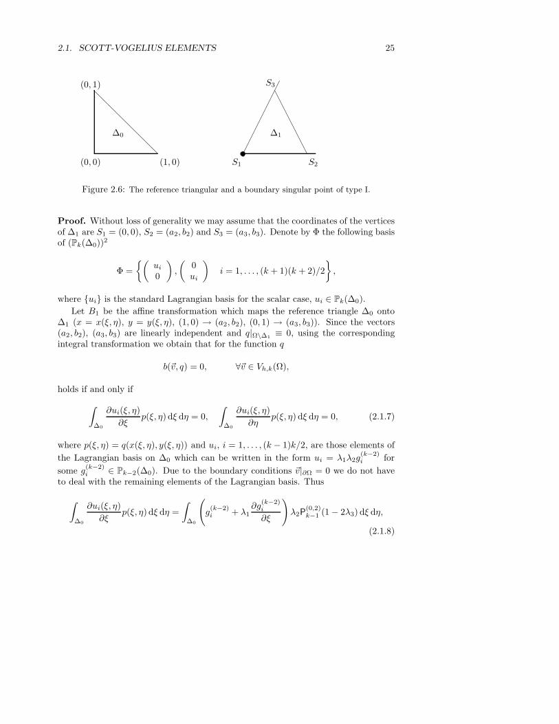
2.1. SCOTT-VOGELIUS ELEMENTS 25
∆0
(0, 1)
(0, 0) (1, 0)
∆1
S1 S2
S3
Figure 2.6: The reference triangular and a boundary singular point of type I.
Proof. Without loss of generality we may assume that the coordinates of the verticesof ∆1 are S1 = (0, 0), S2 = (a2, b2) and S3 = (a3, b3). Denote by Φ the following basisof (Pk(∆0))
2
Φ =
(
ui
0
)
,
(
0ui
)
i = 1, . . . , (k + 1)(k + 2)/2
,
where ui is the standard Lagrangian basis for the scalar case, ui ∈ Pk(∆0).
Let B1 be the affine transformation which maps the reference triangle ∆0 onto∆1 (x = x(ξ, η), y = y(ξ, η), (1, 0) → (a2, b2), (0, 1) → (a3, b3)). Since the vectors(a2, b2), (a3, b3) are linearly independent and q|Ω\∆1
≡ 0, using the correspondingintegral transformation we obtain that for the function q
b(~v, q) = 0, ∀~v ∈ Vh,k(Ω),
holds if and only if
∫
∆0
∂ui(ξ, η)
∂ξp(ξ, η) dξ dη = 0,
∫
∆0
∂ui(ξ, η)
∂ηp(ξ, η) dξ dη = 0, (2.1.7)
where p(ξ, η) = q(x(ξ, η), y(ξ, η)) and ui, i = 1, . . . , (k − 1)k/2, are those elements of
the Lagrangian basis on ∆0 which can be written in the form ui = λ1λ2g(k−2)i for
some g(k−2)i ∈ Pk−2(∆0). Due to the boundary conditions ~v|∂Ω = 0 we do not have
to deal with the remaining elements of the Lagrangian basis. Thus
∫
∆0
∂ui(ξ, η)
∂ξp(ξ, η) dξ dη =
∫
∆0
(
g(k−2)i + λ1
∂g(k−2)i
∂ξ
)
λ2P(0,2)k−1 (1 − 2λ3) dξ dη,
(2.1.8)
26 CHAPTER 2. SOME FINITE ELEMENT FAMILIES
and Theorem 2.1.7 implies (taking there n = k− 1, α = 0, β = 1, γ = 0) that the lastintegral is equal to 0. Similarly, the integral
∫
∆0
∂ui(ξ, η)
∂ηp(ξ, η) dξ dη =
∫
∆0
(
g(k−2)i + λ2
∂g(k−2)i
∂η
)
λ1P(0,2)k−1 (1 − 2λ3) dξ dη
(2.1.9)is equal to 0 (Theorem 2.1.7, n = k − 1, α = 0, β = 0, γ = 1). 2
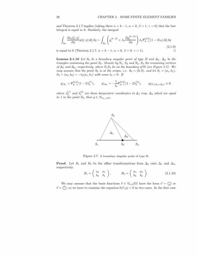
Lemma 2.1.10 Let S0 be a boundary singular point of type II and ∆1, ∆2 be thetriangles containing the point S0. Denote by S1, S2 and S2, S3 the remaining verticesof ∆1 and ∆2, respectively, where S1S3 lie on the boundary of Ω (see Figure 2.7). Wemay assume that the point S0 is at the origin, i.e. S0 = (0, 0), and let S1 = (a1, b1),S3 = (a3, b3) = −t0(a1, b1) with some t0 > 0. If
q|∆1= P
(0,2)k−1 (1 − 2λ
(1)3 ), q|∆2
= −1
t0P
(0,2)k−1 (1 − 2λ
(2)3 ), q|Ω\(∆1∪∆2) ≡ 0,
where λ(1)2 and λ
(2)1 are those barycentric coordinates in ∆1 resp. ∆2 which are equal
to 1 in the point S0, then q ∈ NVh,k(Ω).
∆1∆2
S1 S3
S2
S0
Figure 2.7: A boundary singular point of type II.
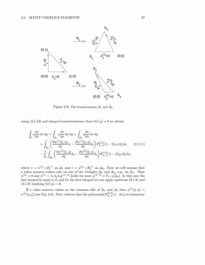
Proof. Let B1 and B2 be the affine transformations from ∆0 onto ∆1 and ∆2,respectively:
B1 =
(
a2 a1
b2 b1
)
, B2 =
(
a3 a2
b3 b2
)
. (2.1.10)
We may assume that the basis functions ~v ∈ Vh,k(Ω) have the form ~v =(
v0
)
or
~v =(
0v
)
, so we have to examine the equation b(~v, q) = 0 in two cases. In the first case
2.1. SCOTT-VOGELIUS ELEMENTS 27
(0,0)
(0,1)
(1,0)
(0,0)S1
S2
(0,0)
S2
S3
B1
B2
λ 1=0
λ2=0
λ3 =0
λ2 (1)=0
λ1(1)=0
λ 3(1) =0
λ1(2) =
0λ
2(2)=0
λ3
(2)=0
Figure 2.8: The transformation B1 and B2
using (2.1.10) and integral transformations, from b(~v, q) = 0 we obtain
∫
Ω
q∂v
∂xdxdy =
∫
∆1
q∂v
∂xdx dy +
∫
∆2
q∂v
∂xdxdy
=
∫
∆0
(
∂u(1)(ξ, η)
∂ξb1 −
∂u(1)(ξ, η)
∂ηb2
)
P(0,2)k−1 (1 − 2λ3) dξ dη (2.1.11)
−1
t0
∫
∆0
(
∂u(2)(ξ, η)
∂ξb2 −
∂u(2)(ξ, η)
∂ηb3
)
P(0,2)k−1 (1 − 2λ3) dξ dη,
where v = u(1) B−11 on ∆1 and v = u(2) B−1
2 on ∆2. First we will assume thatv takes nonzero values only on one of the triangles ∆1 and ∆2, e.g. on ∆1. Thenu(2) ≡ 0 and u(1) = λ1λ2λ3g
(k−3) holds for some g(k−3) ∈ Pk−3(∆0). In this case thelast integral is equal to 0, and for the first integral we can apply equations (2.1.8) and(2.1.9) implying b(~v, q) = 0.
If v takes nonzero values on the common side of ∆1 and ∆2 then u(1)(ξ, η) =
u(2)(η, ξ) (see Fig. 2.8). Now, observe that the polynomial P(0,2)k−1 (1−2λ3) is symmetric
28 CHAPTER 2. SOME FINITE ELEMENT FAMILIES
in ξ and η that implies
∫
∆0
∂u(1)(ξ, η)
∂ξP
(0,2)k−1 (1 − 2λ3) dξ dη =
∫
∆0
∂u(2)(ξ, η)
∂ηP
(0,2)k−1 (1 − 2λ3) dξ dη,
∫
∆0
∂u(1)(ξ, η)
∂ηP
(0,2)k−1 (1 − 2λ3) dξ dη =
∫
∆0
∂u(2)(ξ, η)
∂ξP
(0,2)k−1 (1 − 2λ3) dξ dη.
Since b3 = −t0b1 and since the function u(1) can be written in the form λ1λ3g(k−2)1 ,
(see Fig. 2.8) where g(k−2) ∈ Pk−2(∆0), equation (2.1.11) takes the form
∫
Ω
q∂v
∂xdxdy = −b2
(
1 +1
t0
)∫
∆0
∂u(1)(ξ, η)
∂ηP
(0,2)k−1 (1 − 2λ3) dξ dη
= −b2
(
1 +1
t0
)∫
∆0
(
−g(k−2) + λ3∂g(k−2)
∂ξ
)
λ1P(0,2)k−1 (1 − 2λ3) dξ dη = 0.
(see Theorem 2.1.7 taking n = k − 1, α = 0, β = 0, γ = 1).
In the case ~v =(
0v
)
, the equation b(~v, q) = 0 for the piecewise polynomial q canbe proved in the same way. 2
Lemma 2.1.11 Let S0 be a boundary singular point of type III, and ∆1, ∆2, ∆3 bethe triangles which contain the point S0. Denote by Si, i = 1, 2, 3, 4, the remainingvertices of the triangles ∆i, i = 1, 2, 3 (see Figure 2.9). Here S0S1 and S0S4 areparts of the boundary of Ω. Let S0 = (0, 0) and Si = (ai, bi), i = 1, 2, 3, 4, where(a3, b3) = −t0(a1, b1) and (a4, b4) = −t1(a2, b2) with some t0, t1 > 0. Then thefunction
q|∆1= P
(0,2)k−1 (1 − 2λ
(1)3 ), q|∆2
= −1
t0P
(0,2)k−1 (1 − 2λ
(2)3 ),
q|∆3=
1
t0t1P
(0,2)k−1 (1 − 2λ
(3)3 ), q|Ω\(∆1∪∆2∪∆3
≡ 0,
where λ(1)3 , λ
(2)3 and λ
(3)3 are the coordinates in ∆1, ∆2 and ∆3, respectively, which
are equal to 1 in the point S0, is an element of NVh,k(Ω).
Proof. To obtain the statement of the lemma we apply the argumentation of Lemma2.1.10 to ∆1, ∆2 and to ∆2, ∆3. 2
Lemma 2.1.12 Let S0 be a boundary singular point of type IV, and ∆i, i = 1, 2, 3, 4,be the triangles which contain the point S0. Denote by Si, i = 1, . . . , 5, the remainingvertices of the triangles ∆i, i = 1, 2, 3, 4 (see Figure 2.9). Here S0S4S5 is a part ofthe boundary of Ω. Let S0 = (0, 0) and Si = (ai, bi), i = 1, . . . , 5, where (a3, b3) =
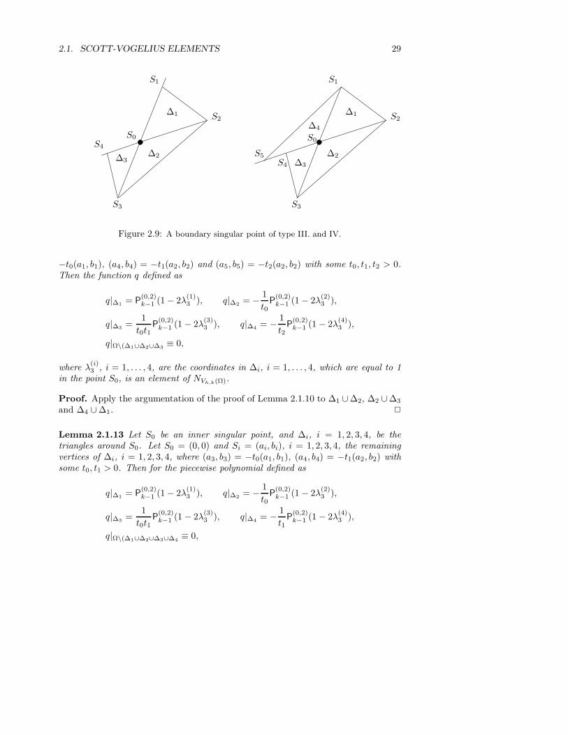
2.1. SCOTT-VOGELIUS ELEMENTS 29
S1
S2
S3
S4
S0
∆1
∆2∆3
S1
S2
S3
S4
S0
S5
∆1
∆2∆3
∆4
Figure 2.9: A boundary singular point of type III. and IV.
−t0(a1, b1), (a4, b4) = −t1(a2, b2) and (a5, b5) = −t2(a2, b2) with some t0, t1, t2 > 0.Then the function q defined as
q|∆1= P
(0,2)k−1 (1 − 2λ
(1)3 ), q|∆2
= −1
t0P
(0,2)k−1 (1 − 2λ
(2)3 ),
q|∆3=
1
t0t1P
(0,2)k−1 (1 − 2λ
(3)3 ), q|∆4
= −1
t2P
(0,2)k−1 (1 − 2λ
(4)3 ),
q|Ω\(∆1∪∆2∪∆3≡ 0,
where λ(i)3 , i = 1, . . . , 4, are the coordinates in ∆i, i = 1, . . . , 4, which are equal to 1
in the point S0, is an element of NVh,k(Ω).
Proof. Apply the argumentation of the proof of Lemma 2.1.10 to ∆1 ∪∆2, ∆2 ∪∆3
and ∆4 ∪ ∆1. 2
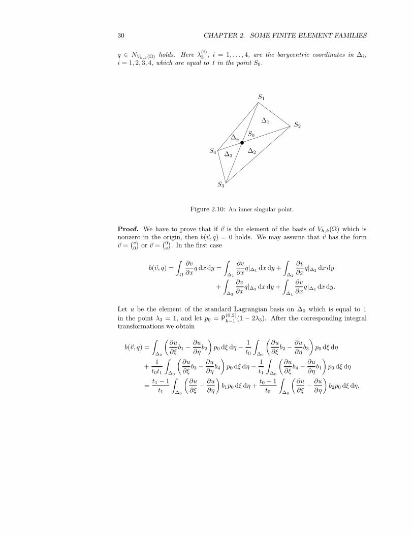
Lemma 2.1.13 Let S0 be an inner singular point, and ∆i, i = 1, 2, 3, 4, be thetriangles around S0. Let S0 = (0, 0) and Si = (ai, bi), i = 1, 2, 3, 4, the remainingvertices of ∆i, i = 1, 2, 3, 4, where (a3, b3) = −t0(a1, b1), (a4, b4) = −t1(a2, b2) withsome t0, t1 > 0. Then for the piecewise polynomial defined as
q|∆1= P
(0,2)k−1 (1 − 2λ
(1)3 ), q|∆2
= −1
t0P
(0,2)k−1 (1 − 2λ
(2)3 ),
q|∆3=
1
t0t1P
(0,2)k−1 (1 − 2λ
(3)3 ), q|∆4
= −1
t1P
(0,2)k−1 (1 − 2λ
(4)3 ),
q|Ω\(∆1∪∆2∪∆3∪∆4≡ 0,
30 CHAPTER 2. SOME FINITE ELEMENT FAMILIES
q ∈ NVh,k(Ω) holds. Here λ(i)3 , i = 1, . . . , 4, are the barycentric coordinates in ∆i,
i = 1, 2, 3, 4, which are equal to 1 in the point S0.
S1
S2
S4
S3
S0
∆1
∆2∆3
∆4
Figure 2.10: An inner singular point.
Proof. We have to prove that if ~v is the element of the basis of Vh,k(Ω) which isnonzero in the origin, then b(~v, q) = 0 holds. We may assume that ~v has the form~v =
(
v0
)
or ~v =(
0v
)
. In the first case
b(~v, q) =
∫
Ω
∂v
∂xq dx dy =
∫
∆1
∂v
∂xq|∆1
dx dy +
∫
∆2
∂v
∂xq|∆2
dxdy
+
∫
∆3
∂v
∂xq|∆3
dxdy +
∫
∆4
∂v
∂xq|∆4
dxdy.
Let u be the element of the standard Lagrangian basis on ∆0 which is equal to 1
in the point λ3 = 1, and let p0 = P(0,2)k−1 (1 − 2λ3). After the corresponding integral
transformations we obtain
b(~v, q) =
∫
∆0
(
∂u
∂ξb1 −
∂u
∂ηb2
)
p0 dξ dη −1
t0
∫
∆0
(
∂u
∂ξb2 −
∂u
∂ηb3
)
p0 dξ dη
+1
t0t1
∫
∆0
(
∂u
∂ξb3 −
∂u
∂ηb4
)
p0 dξ dη −1
t1
∫
∆0
(
∂u
∂ξb4 −
∂u
∂ηb1
)
p0 dξ dη
=t1 − 1
t1
∫
∆0
(
∂u
∂ξ−
∂u
∂η
)
b1p0 dξ dη +t0 − 1
t0
∫
∆0
(
∂u
∂ξ−
∂u
∂η
)
b2p0 dξ dη,

2.1. SCOTT-VOGELIUS ELEMENTS 31
where we have used that (a3, b3) = −t0(a1, b1) and (a4, b4) = −t1(a2, b2). Similarly,if ~v =
(
0v
)
holds then
b(~v, q) =
∫
Ω
∂v
∂yq dxdy =
t1 − 1
t1
∫
∆0
(
∂u
∂η−
∂u
∂ξ
)
a1p0 dξ dη+
t0 − 1
t0
∫
∆0
(
∂u
∂η−
∂u
∂ξ
)
a2p0 dξ dη.
As u and p0 are functions of λ3 = 1 − ξ − η, we have∫
∆0
∂u
∂ξp0 dξ dη =
∫
∆0
∂u
∂ηp0 dξ dη
which implies b(~v, q) = 0. 2
Proof of Theorem 2.1.8. We will prove that the constant function and the functionsfrom NVh,k(Ω) described in Lemmas 2.1.6–2.1.13 (corresponding to the singular pointsof Th) are linearly independent. Since the functions in Lemmas 2.1.6–2.1.13 havenonzero values only in the triangles around the considered singular point we have toexamine only the cases when a triangle contains more than 1 singular point.
We give two versions of the proof: the first is valid only in the case when all thetriangles in Th contain at most two singular points, while the second one is valid inall cases.1. version. Let ∆ ∈ Th be a triangle with vertices Si, i = 1, 2, 3. Denote by λi
that barycentric coordinate in ∆ which is equal to 1 in Si, i = 1, 2, 3, respectively.We will assume that S1 and S2 are singular points of Th. Denote by q1 and q2 thecorresponding element of NVh,k(Ω) and let q3 ≡ 1. In this case we may assume
q1|∆ = P(0,2)k−1 (1 − 2λ1), q2|∆ = P
(0,2)k−1 (1 − 2λ2).
Let A ∈ R3×3 be a matrix such that aij is equal to the value of qi in the point Sj ,
i, j = 1, 2, 3. Then using (2.1.4) we obtain
A =
P(0,2)k−1 (−1) P
(0,2)k−1 (1) P
(0,2)k−1 (1)
P(0,2)k−1 (1) P
(0,2)k−1 (−1) P
(0,2)k−1 (1)
1 1 1
=
a 1 11 a 11 1 1
,
where a = (−1)k−1k(k + 1)/2. It follows from det(A) = (a − 1)2 that the functionsqi, i = 1, 2, 3, are linearly independent if k > 1. 2
2. version. Let ∆ ∈ Th be a triangle with vertices Si, i = 1, 2, 3. Denote by λi thatbarycentric coordinate in ∆ which is equal to 1 in Si, i = 1, 2, 3, respectively. We willassume that all the vertices of ∆ are singular points in Th. Denote by qi, i = 1, 2, 3,the corresponding element of NVh,k(Ω), and let q4 ≡ 1. In this case we may assume
qi|∆ = P(0,2)k−1 (1 − 2λi), i = 1, 2, 3.
32 CHAPTER 2. SOME FINITE ELEMENT FAMILIES
If there exist constants αi, i = 1, 2, 3, such that
3∑
i=1
αiqi|∆ = q4|∆
holds, then3∑
i=1
αi
∫
∆
qi|∆λ1λ2λ3 dx dy =
∫
∆
λ1λ2λ3 dxdy.
After the corresponding integral transformations we obtain
3∑
i=1
αi
∫
∆0
P(0,2)k−1 (1 − 2λ
(0)i )λ
(0)1 λ
(0)2 λ
(0)3 dξ dη =
∫
∆0
λ(0)1 λ
(0)2 λ
(0)3 dξ dη, (2.1.12)
where we used notations λ(0)i , i = 1, 2, 3, to denote the barycentric coordinates in ∆0
(this notation differs from the usual one). It follows from Lemma 1.4.7 that the lastintegral is equal to 1
5! and
∫
∆0
P(0,2)k−1 (1 − 2λ
(0)i )λ
(0)1 λ
(0)2 λ
(0)3 dξ dη =
∫
∆0
P(0,2)k−1 (1 − 2λ
(0)3 )λ
(0)1 λ
(0)2 λ
(0)3 dξ dη
holds for i = 1, 2, 3. Since k ≥ 4, Theorem 2.1.7 implies (taking there n = k − 1,α = β = 0, γ = 1) that
∫
∆0
P(0,2)k−1 (1 − 2λ
(0)3 )λ
(0)1 λ
(0)2 λ
(0)3 dξ dη = 0,
which contradicts to (2.1.12). That means the functions qi, i = 1, 2, 3, 4 are linearlyindependent. 2
The lower order cases. In Lemmas 2.1.6–2.1.13 we do not use the condition k ≥ 4,the results remain valid for the lower order cases, too. In both proofs of Theorem 2.1.8to prove that the functions described in Lemmas 2.1.6–2.1.13 are linearly independent,it suffices to consider a weaker condition for k. In the first proof we used only thecondition k > 1. In the second proof we need a lower bound for k only in order toapply Theorem 2.1.7, however for our purposes it is sufficient to require k > 2. Thismeans that the constant function and the functions defined in Lemmas 2.1.6–2.1.13are linearly independent for all k > 2, and for all k > 1 in the case when all thetriangles contain at most two singular points. The condition k ≥ 4 is important whenwe apply Lemma 2.1.5 in the proof of Theorem 2.1.8: in the lower order cases thedimension of the nullspace can be greater than σ + 1.
2.1. SCOTT-VOGELIUS ELEMENTS 33
S1S2
S3
S4S5
S6
S7
P
Figure 2.11: A domain Ω and a triangulation where NVh.2(Ω) ≥ N − 2 = 5
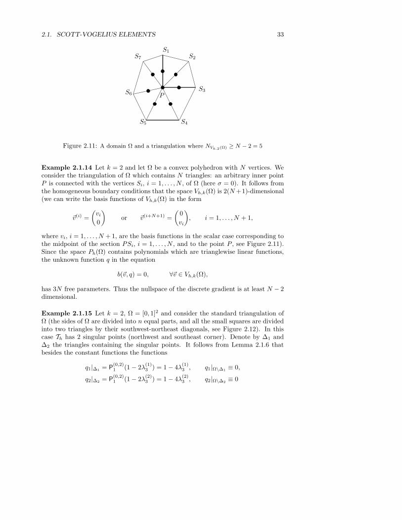
Example 2.1.14 Let k = 2 and let Ω be a convex polyhedron with N vertices. Weconsider the triangulation of Ω which contains N triangles: an arbitrary inner pointP is connected with the vertices Si, i = 1, . . . , N , of Ω (here σ = 0). It follows fromthe homogeneous boundary conditions that the space Vh,k(Ω) is 2(N +1)-dimensional(we can write the basis functions of Vh,k(Ω) in the form
~v(i) =
(
vi
0
)
or ~v(i+N+1) =
(
0
vi
)
, i = 1, . . . , N + 1,
where vi, i = 1, . . . , N + 1, are the basis functions in the scalar case corresponding tothe midpoint of the section PSi, i = 1, . . . , N , and to the point P , see Figure 2.11).Since the space Ph(Ω) contains polynomials which are trianglewise linear functions,the unknown function q in the equation
b(~v, q) = 0, ∀~v ∈ Vh,k(Ω),
has 3N free parameters. Thus the nullspace of the discrete gradient is at least N − 2dimensional.
Example 2.1.15 Let k = 2, Ω = [0, 1]2 and consider the standard triangulation ofΩ (the sides of Ω are divided into n equal parts, and all the small squares are dividedinto two triangles by their southwest-northeast diagonals, see Figure 2.12). In thiscase Th has 2 singular points (northwest and southeast corner). Denote by ∆1 and∆2 the triangles containing the singular points. It follows from Lemma 2.1.6 thatbesides the constant functions the functions
q1|∆1= P
(0,2)1 (1 − 2λ
(1)3 ) = 1 − 4λ
(1)3 , q1|Ω\∆1
≡ 0,
q2|∆2= P
(0,2)1 (1 − 2λ
(2)3 ) = 1 − 4λ
(2)3 , q2|Ω\∆2
≡ 0
34 CHAPTER 2. SOME FINITE ELEMENT FAMILIES
are in the nullspace of the discrete gradient operator. Here λ(1)3 and λ
(2)3 are the
barycentric coordinates in ∆1 and ∆2, which are equal to 1 in the correspondingsingular points.
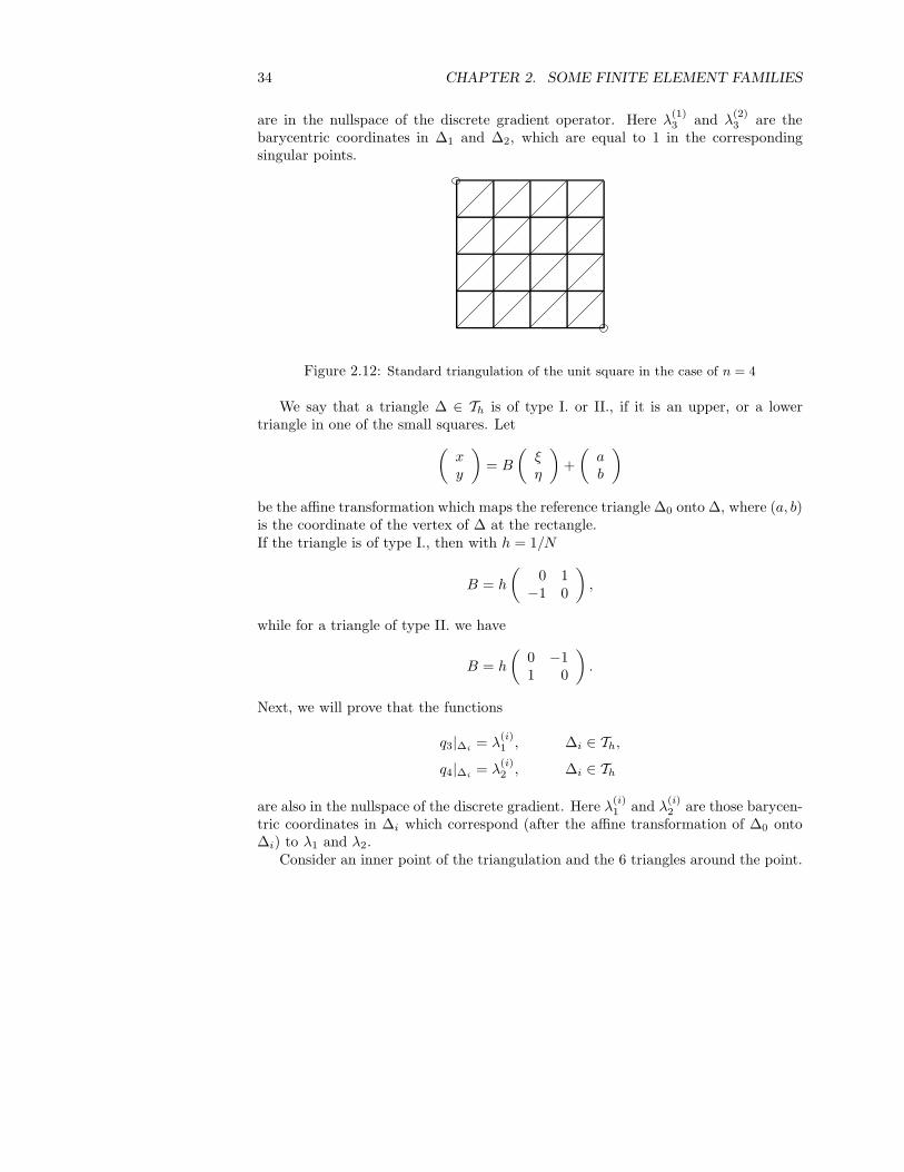
Figure 2.12: Standard triangulation of the unit square in the case of n = 4
We say that a triangle ∆ ∈ Th is of type I. or II., if it is an upper, or a lowertriangle in one of the small squares. Let
(
xy
)
= B
(
ξη
)
+
(
ab
)
be the affine transformation which maps the reference triangle ∆0 onto ∆, where (a, b)is the coordinate of the vertex of ∆ at the rectangle.If the triangle is of type I., then with h = 1/N
B = h
(
0 1−1 0
)
,
while for a triangle of type II. we have
B = h
(
0 −11 0
)
.
Next, we will prove that the functions
q3|∆i= λ
(i)1 , ∆i ∈ Th,
q4|∆i= λ
(i)2 , ∆i ∈ Th
are also in the nullspace of the discrete gradient. Here λ(i)1 and λ
(i)2 are those barycen-
tric coordinates in ∆i which correspond (after the affine transformation of ∆0 onto∆i) to λ1 and λ2.
Consider an inner point of the triangulation and the 6 triangles around the point.

2.1. SCOTT-VOGELIUS ELEMENTS 35
~u3
~u1 ~u2
~u4
∆6
∆7
∆8
∆5
∆4
∆3
It suffices to prove that∫
Ω
qj div ~ui dxdy = 0, j = 3, 4, i = 1, 2, 3, 4, (2.1.13)
where ~ui ∈ Vh,k, i = 1, 2, 3, 4, are the basis functions belonging to the points drawnon the figure and ~ui =
(
u0
)
or ~ui =(
0u
)
, where u is the corresponding element of thelocal basis.
In the scalar case the standard Lagrangian basis on ∆0 is:
v1 = λ3(2λ3 − 1),
v2 = 4λ3λ2,
v3 = λ2(2λ2 − 1),
v4 = 4λ3λ1,
v5 = 4λ1λ2,
v6 = λ1(2λ1 − 1).
For vectors ~u2, ~u3 and ~u4 equality (2.1.13) holds since these functions have nonzerovalues only in two adjacent triangles, where one of the triangles is of type I. andthe other is of type II. Further, transforming these two triangles onto ∆0 the veloc-ity functions in the two triangles belonging to the nodal point on the common sidecorrespond to the same element of the local basis in ∆0.
E.g. if i = 3, j = 3 using that the triangles ∆3 and ∆4 is of type I. and II.,respectively, we obtain
∫
Ω
q3∂~u3
∂xdx dy =
∫
∆3
λ(3)1
∂~u3
∂xdxdy +
∫
∆4
λ(4)1
∂~u3
∂xdxdy
= h
∫
∆0
λ1∂v5
∂ηdξ dη − h
∫
∆0
λ1∂v5
∂ηdξ dη = 0.
Here v5 = 4λ1λ2 is the corresponding element of the local basis on ∆0. Similarly∫
Ω
q3∂~u3
∂ydx dy =
∫
∆3
λ(3)1
∂~u3
∂ydxdy +
∫
∆4
λ(4)1
∂~u3
∂ydxdy
= h
∫
∆0
λ1∂v5
∂ξdξ dη − h
∫
∆0
λ1∂v5
∂ξdξ dη = 0.

36 CHAPTER 2. SOME FINITE ELEMENT FAMILIES
In the case of ~u1 in a similar way we obtain that for j = 3, 4∫
∆3∪∆6
qj div ~u1 dxdy = 0,
∫
∆4∪∆7
qj div ~u1 dx dy = 0,
∫
∆5∪∆8
qj div ~u1 dxdy = 0.
From the reasoning above we obtain that the nullspace is at least σ + 3 dimensional.
Example 2.1.16 If k = 2 and Ω = [0, 1]2 then in the case of the criss-cross grid,similarly to the cases k ≥ 4, the nullspace is σ + 1 dimensional.
Example 2.1.17 If k = 3, Ω is a convex polyhedron with N vertices and we considerthe same triangulation of Ω as in Example 2.1.14, then we obtain that the nullspaceis at least 2 dimensional (here σ = 0).
2.2 Fortin-Soulie element
A possibility to avoid the unpleasant grid condition mentioned in Section 2.1 is en-larging the velocity space Vh(Ω).
The idea is coming from [13], where a second order non-conforming finite elementpair was investigated. In that paper the continuity of the discrete velocities betweenthe triangles is not assumed, the continuity is required only in the second order Gauss-Legendre points. The corresponding discrete spaces are
Ph(Ω) = p ∈ L2(Ω), p|∆ ∈ P1(∆), ∆ ∈ Th (2.2.1)
V nch,2(Ω) =
~v ∈ (L2(Ω))2, ~v|∆ ∈ (P2(∆))2, and ~v is continuous in all
2nd-order Gauss-Legendre points of all sides of ∆, ∆ ∈ Th , (2.2.2)
the norm in Vh,2 being defined as |~vh|1,h :=
(
∑
∆∈Th
|~vh|21,∆
)1/2
.
It is understood that in this case instead of homogeneous boundary conditions thevelocity components vℓ, ℓ = 1, 2, satisfy
∫
E
qvℓ ds = 0, q ∈ P1(E)
for all edges E ⊂ ∂∆ ∩ ∂Ω and for all ∆ ∈ Th.Let ∆ ∈ Th be a given triangle, and denote by λ1, λ2, λ3 the barycentric coordi-
nates in ∆. Then on the sides of ∆ the function
b∆ := 3(λ21 + λ2
2 + λ23) − 2 (2.2.3)

2.2. FORTIN-SOULIE ELEMENT 37
0
0.5
1
0
0.5
1−1
−0.5
0
0.5
1
Figure 2.13: The function b∆ on the reference triangle.
is equal to the second order Legendre polynomial; b∆ disappears in the second orderGauss-Legendre points on the sides of ∆. From this follows that one gets the velocityspace (2.2.2) by adding trianglewise this function to the conforming velocity spaceVh,2(Ω):
V nch,2(Ω) = Vh,2(Ω) +
~v, ~v|∆ =
(
α∆
β∆
)
b∆, α∆, β∆ ∈ R, ∆ ∈ Th
.
The authors announced that the element pair (2.2.1)–(2.2.2) is inf-sup stable with-out a restriction on the grid.
Lemma 2.2.1 In the case of the finite element (2.2.1)–(2.2.2) the nullspace of thediscrete gradient is one-dimensional, it contains only constant functions.
Proof. Let q ∈ Ph be a function for which b(~v, q) = 0 holds for all ~v ∈ V nch,2, and let
∆ ∈ Th be a triangle from the support of q. Let ~v|∆ =(
b∆0
)
, ~v|Ω\∆ ≡ 0, then using
38 CHAPTER 2. SOME FINITE ELEMENT FAMILIES
that ∂q∂x1
≡ const we obtain
0 = b(~v, q) = −
∫
∆
∂q
∂x1b∆ dx = −
∂q
∂x1
∫
∆
b∆ dx =∂q
∂x1·1
4,
which means that ∂q∂x1
≡ 0. Similarly, we have ∂q∂x2
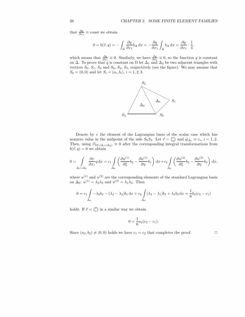
≡ 0, so the function q is constanton ∆. To prove that q is constant on Ω let ∆1 and ∆2 be two adjacent triangles withvertices S0, S1, S2 and S0, S2, S3, respectively (see the figure). We may assume thatS0 = (0, 0) and let Si = (ai, bi), i = 1, 2, 3.
∆2
∆1
S3 S0
S1
S2
Denote by v the element of the Lagrangian basis of the scalar case which hasnonzero value in the midpoint of the side S0S2. Let ~v =
(
v0
)
and q|∆i≡ ci, i = 1, 2.
Then, using ~v|Ω\(∆1∪∆2) ≡ 0 after the corresponding integral transformations fromb(~v, q) = 0 we obtain
0 =
∫
∆1∪∆2
∂v
∂x1q dx = c1
∫
∆0
(
∂u(1)
∂ξb2 −
∂u(1)
∂ηb1
)
dx+c2
∫
∆0
(
∂u(2)
∂ξb3 −
∂u(2)
∂ηb2
)
dx,
where u(1) and u(2) are the corresponding elements of the standard Lagrangian basison ∆0: u(1) = λ2λ3 and u(2) = λ1λ3. Then
0 = c1
∫
∆0
−λ2b2 − (λ3 − λ2)b1 dx + c2
∫
∆0
(λ3 − λ1)b3 + λ1b2 dx =1
6b2(c2 − c1)
holds. If ~v =(
0v
)
in a similar way we obtain
0 =1
6a2(c2 − c1).
Since (a2, b2) 6= (0, 0) holds we have c1 = c2 that completes the proof. 2
2.3. SOME HIGHER ORDER NON-CONFORMING FINITE ELEMENTS 39
2.3 Some higher order non-conforming finite ele-
ments
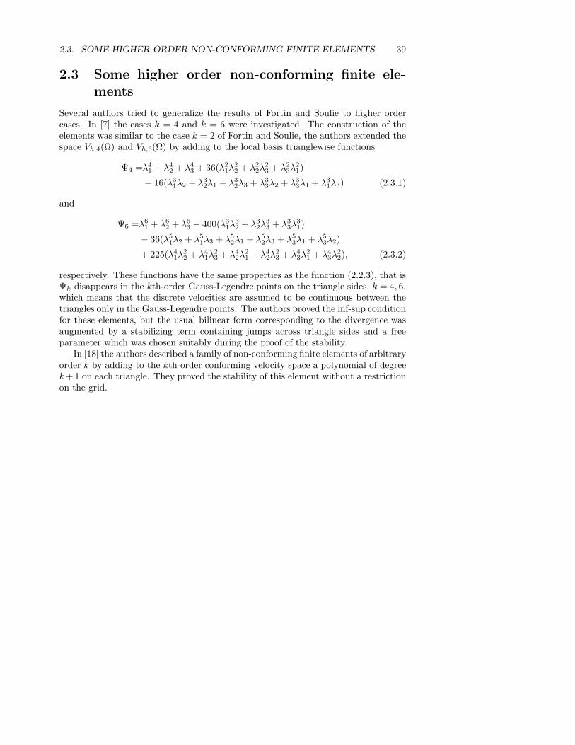
Several authors tried to generalize the results of Fortin and Soulie to higher ordercases. In [7] the cases k = 4 and k = 6 were investigated. The construction of theelements was similar to the case k = 2 of Fortin and Soulie, the authors extended thespace Vh,4(Ω) and Vh,6(Ω) by adding to the local basis trianglewise functions
Ψ4 =λ41 + λ4
2 + λ43 + 36(λ2
1λ22 + λ2
2λ23 + λ2
3λ21)
− 16(λ31λ2 + λ3
2λ1 + λ32λ3 + λ3
3λ2 + λ33λ1 + λ3
1λ3) (2.3.1)
and
Ψ6 =λ61 + λ6
2 + λ63 − 400(λ3
1λ32 + λ3
2λ33 + λ3
3λ31)
− 36(λ51λ2 + λ5
1λ3 + λ52λ1 + λ5
2λ3 + λ53λ1 + λ5
3λ2)
+ 225(λ41λ
22 + λ4
1λ23 + λ4
2λ21 + λ4
2λ23 + λ4
3λ21 + λ4
3λ22), (2.3.2)
respectively. These functions have the same properties as the function (2.2.3), that isΨk disappears in the kth-order Gauss-Legendre points on the triangle sides, k = 4, 6,which means that the discrete velocities are assumed to be continuous between thetriangles only in the Gauss-Legendre points. The authors proved the inf-sup conditionfor these elements, but the usual bilinear form corresponding to the divergence wasaugmented by a stabilizing term containing jumps across triangle sides and a freeparameter which was chosen suitably during the proof of the stability.
In [18] the authors described a family of non-conforming finite elements of arbitraryorder k by adding to the kth-order conforming velocity space a polynomial of degreek +1 on each triangle. They proved the stability of this element without a restrictionon the grid.

40 CHAPTER 2. SOME FINITE ELEMENT FAMILIES

Chapter 3
Gauss-Legendre elements
In this chapter we define a non-conforming finite element family of arbitrary orderk, and we prove its inf-sup stability for any even k without assumptions on the grid.This family generalizes the well-known low-order cases, k = 1 (Crouzeix-Raviart[11]), k = 2 (Fortin-Soulie [13]), k = 3 (Crouzeix-Falk [10]), where non-conformingapproximations for the velocities are used.
3.1 Definitions and properties
Definition 3.1.1 (See in [30]) We define the non-conforming kth-order Gauss-Le-gendre element on Ω as
Ph(Ω) =
p ∈ L2(Ω), p|∆ ∈ Pk−1(∆), ∆ ∈ Th
(3.1.1)
V nch,k(Ω) =
~v ∈ (L2(Ω))2, ~v|∆ ∈ (Pk(∆))2, and ~v is continuous in all
kth-order Gauss-Legendre points of all sides of ∆, ∆ ∈ Th, ~v = 0 in
all kth-order Gauss-Leg. points on the triangle sides E ⊂ Γ , (3.1.2)
the norm in V nch,k being defined as |~vh|1,h,Ω :=
(
∑
∆∈Th
|~vh|21,∆
)1/2
.
As we mentioned in Section 1.6 the continuity in the Gauss-Legendre points indicatesthat the patch-test is fulfilled, i.e. the seminorm |.|1,h,Ω is a norm on V nc
h,k(Ω).
The question we consider next is to specify of suitable degrees of freedom for thevelocity parts of these elements.
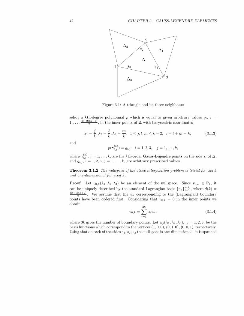
Consider a fixed triangle ∆ with barycentric coordinates λ1, λ2, λ3 and sidess1, s2, s3, see Figure 3.1. We will examine the following interpolation problem:
41
42 CHAPTER 3. GAUSS-LEGENDRE ELEMENTS
s3
s2
s1
3
2
1
∆3
∆2∆1
∆
Figure 3.1: A triangle and its three neighbours
select a kth-degree polynomial p which is equal to given arbitrary values gi, i =
1, . . . , (k−2)(k−1)2 , in the inner points of ∆ with barycentric coordinates
λ1 =j
k, λ2 =
ℓ
k, λ3 =
m
k, 1 ≤ j, ℓ, m ≤ k − 2, j + ℓ + m = k, (3.1.3)
andp(γ
(k)i,j ) = gi,j i = 1, 2, 3, j = 1, . . . , k,
where γ(k)i,j , j = 1, . . . , k, are the kth-order Gauss-Legendre points on the side si of ∆,
and gi,j , i = 1, 2, 3, j = 1, . . . , k, are arbitrary prescribed values.
Theorem 3.1.2 The nullspace of the above interpolation problem is trivial for odd kand one-dimensional for even k.
Proof. Let v0,k(λ1, λ2, λ3) be an element of the nullspace. Since v0,k ∈ Pk, it
can be uniquely described by the standard Lagrangian basis wid(k)i=1 , where d(k) =
(k+1)(k+2)2 . We assume that the wi corresponding to the (Lagrangian) boundary
points have been ordered first. Considering that v0,k = 0 in the inner points weobtain
v0,k =3k∑
i=1
αiwi, (3.1.4)
where 3k gives the number of boundary points. Let wj(λ1, λ2, λ3), j = 1, 2, 3, be thebasis functions which correspond to the vertices (1, 0, 0), (0, 1, 0), (0, 0, 1), respectively.Using that on each of the sides s1, s2, s3 the nullspace is one-dimensional – it is spanned
3.1. DEFINITIONS AND PROPERTIES 43
by the kth-degree Legendre-polynomial Lk(s) – and Lk(1) =: c 6= 0, Lk(0) = (−1)kc,on the side s1 (where λ1 = 0, λ2 = 1 − s, λ3 = s, s ∈ [0, 1]) we have v0,k|s1
= αLk(s)for some constant α and can write
v0,k(0, 0, 1) = αLk(1) = αc = α3w3(0, 0, 1),
v0,k(0, 1, 0) = αLk(0) = α(−1)kc = α2w2(0, 1, 0).
Using the same reasoning on s2 and remarking that in the starting point (0, 0, 1),where s = 0, the value αc is already known, we have v0,k|s2
= α(−1)kLk(s) and
v0,k(1, 0, 0) = α(−1)kc.
Finally, continuing on s3, we find that v0,k takes the same values in the two endpointsof s3 which means α = 0 for odd values of k. Hence, v0,k disappears on all sidesof the triangle. This together with (3.1.4) implies v0,k ≡ 0. For even k, we havev0,k = αLk(s) on all three sides (which determines it uniquely in the form (3.1.4)),and hence the nullspace is one-dimensional. 2
Based on the theorem above we can described a basis of V nch,k(Ω) as follows.
Proposition 3.1.3 For even k we can start from a standard Lagrangian basis inevery ∆ including its boundary. The resulting finite element velocities are continuouseverywhere. Moreover, on each triangle there exists a nontrivial polynomial v0,k oforder k such that on the sides of the corresponding triangle it is equal to a multiple ofthe kth-order Legendre polynomial defined on the given side. By adding this polynomialtrianglewise to the Lagrangian basis we obtain trianglewise k-th order polynomials thatare continuous on the common sides of two adjacent triangles in all the kth-orderGauss-Legendre points.
Proof. The first part of the proposition follows from Remark 1.4.8. The existence ofthe nontrivial polynomial v0,k follows from Theorem 3.1.2. 2
Proposition 3.1.4 For odd k, based on the above theorem, inside the triangles wecan use a standard Lagrangian basis whereas on the triangle sides the Gauss-Legendrepoints can be taken as degrees of freedom.
In what follows we establish a form of the basis for the (components of the) velocityspace for any k which is suitable for our subsequent considerations, and we look oncemore on the above interpolation problem with the aim to show that the problem arenot specially the Gauss-Legendre points.
On a fixed triangle ∆, such a basis can be defined as follows:
a) The basis functions corresponding to degrees of freedom connected with innerpoints of ∆ appear for k ≥ 3 and can be represented as
B(3)c,∆q
(k−3)i , i = 1, . . . ,
(k − 2)(k − 1)
2, (3.1.5)
44 CHAPTER 3. GAUSS-LEGENDRE ELEMENTS
where B(3)c,∆ := λ1λ2λ3 is the conforming bubble function of degree 3 and q
(k−3)i =
q(k−3)i (λ1, λ2, λ3) are polynomials of degree k − 3 disappearing in all but one of the
(k−2)(k−1)2 inner points of ∆ with barycentric coordinates (3.1.3). Observe that
(k−2)(k−1)2 is also the number of free parameters of a polynomial of degree k − 3.
Therefore the basis functions corresponding to inner points are well defined by (3.1.5).
b) There remain (k+2)(k+1)2 − (k−2)(k−1)
2 = 3k degrees of freedom on the sides of∆, on each of which they are connected (through the corresponding barycentric coor-dinate) to k knots γj
kj=1 in (0, 1) which we assume to be distributed symmetrically
with respect to 12 . These knots define the polynomials ωk(s) :=
∏kj=1(s − γj) and
ω2,k−1 :=∏k
j=2(s − γj).For the basis functions of ∆ corresponding to any side si we can write
w = w(λ1, λ2, λ3) = αωk(λi) + βωk(λi+1) + γωk(λi+2) + λi+1λi+2q(k−2)(λ1, λ2, λ3),
(3.1.6)where the barycentric coordinates are numbered cyclically (λ4 = λ1, λ5 = λ2), andq(k−2) are suitable polynomials of degree k−2. Further, restricting w to, say, the sides1, i.e. the side on which λ1 = 0, λ2 = 1 − s, λ3 = s, we get
w = w(s) = αωk(0) + βωk(1 − s) + γωk(s) + s(1 − s)q(k−2)(s). (3.1.7)
We shall clarify under which conditions the polynomials given by (3.1.7) can takeevery prescribed value in the knots γjk
j=1 on side s1. In these points, due to their
symmetry with respect to 12 , both polynomials ωk(1 − s) and ωk(s) are zero, and
therefore the degrees of freedom β, γ obviously belong to the other sides of ∆.
For the remaining part a+s(1−s)q(k−2)i (s) (where a := αωk(0), and here ωk(0) 6=
0) we have the following result.
Lemma 3.1.5 The interpolation problem of selecting a constant a and a polynomialq(k−2) of order (k − 2) to arbitrary values g1, . . . , gk prescribed in the knots γjk
j=1
which are symmetrically distributed in (0, 1):
(a + s(1 − s)q(k−2)(s))|s=γj= gj, j = 1, . . . , k, (3.1.8)
is uniquely solvable iff the following conditions are satisfied:1) the knots γj are pairwise different from each other;2) k is odd.
Proof. We denote the determinant of the problem by W (γ1, . . . , γk) = W1,...,k, thatis
W1,...,k :=
∣
∣
∣
∣
∣
∣
1 γ1(1 − γ1) . . . γk−11 (1 − γ1)
. . . . . . . . . . . .
1 γk(1 − γk) . . . γk−1k (1 − γk)
∣
∣
∣
∣
∣
∣
.

3.1. DEFINITIONS AND PROPERTIES 45
By subtracting the first row from the other rows and by subsequent simplificationswe obtain
W1,...,k =k∏
ℓ=2
(γℓ − γ1)
∣
∣
∣
∣
∣
∣
1 − γ1 − γ2 γ2(1 − γ2) . . . γk−22 (1 − γ2)
. . . . . . . . . . . .
1 − γ1 − γk γk(1 − γk) . . . γk−2k (1 − γk)
∣
∣
∣
∣
∣
∣
=
k∏
ℓ=2
(γℓ − γ1)
(1 − γ1)W2,...,k −
−k∏
ℓ=2
γℓ
∣
∣
∣
∣
∣
∣
1 1 − γ2 γ2(1 − γ2) . . . γk−32 (1 − γ2)
. . . . . . . . . . . .
1 1 − γk γk(1 − γk) . . . γk−3k (1 − γk)
∣
∣
∣
∣
∣
∣
=
k∏
ℓ=2
(γℓ − γ1)
(1 − γ1)W2,...,k + (−1)k−1k∏
ℓ=2
γℓ
∏
2≤m<ℓ≤k
(γℓ − γm)
,
where in the last step the formula for Vandermonde determinants has been used.This recursion for W1,...,k, in the special case k = 2, gives already
W1,2 = (γ2 − γ1)(1 − γ1 − γ2) = (γ2 − γ1) ω2(1) − ω2(0) .
The general case then follows by induction remarking that
(1 − γ1) ω2,k−1(1) − ω2,k−1(0) + (−1)k−1k∏
ℓ=2
γℓ = ωk(1) − ωk(0).
Finally,
W1,...,k =∏
1≤m<ℓ≤k
(γℓ − γm) ωk(1) − ωk(0) ,
that completes the proof of the lemma, since, due to the symmetry we have ωk(1) =∏k
j=1 γj = (−1)kωk(0). 2
In what follows for odd k we give an explicit form of the basis functions correspondingto the boundary points of ∆. Similarly to Lemma 3.1.5 let γi, i = 1, . . . , k be pairwisedifferent real numbers which are symmetrically distributed in (0, 1). Since k is oddwe have
γ k+1
2
=1
2, γk−j = 1 − γj , j = 1, . . . ,
k − 1
2.
Consider the following points on the sides of the triangle:
γ(k)1,j = (0, 1 − γj , γj), j = 1, . . . , k, on the side s1,
γ(k)2,j = (γj , 0, 1 − γj), j = 1, . . . , k, on the side s2,
γ(k)3,j = (1 − γj , γj , 0), j = 1, . . . , k, on the side s3.
46 CHAPTER 3. GAUSS-LEGENDRE ELEMENTS
Theorem 3.1.6 Let 1 ≤ j ≤ k−12 , so we have γj = 1
2 − aj and γk−j = 12 + aj with
some aj ∈ (0, 1/2). For i = 1, 2, 3, and j = 1, . . . , k−12 let the piecewise polynomials
q(k)i,j and q
(k)i,k−j be defined as
q(k)i,j (λ1, λ2, λ3) := (3.1.9)
(λi+1λi+2(λi+2 + Aj) + Bj)
(k−1)/2∏
ℓ=1
ℓ 6=j
(λi+1λi+2 − γℓγk−ℓ) − Cj
+
Cj
ωk(0)ωk(λi),
q(k)i,k−j(λ1, λ2, λ3) := (3.1.10)
(λi+1λi+2(λi+1 + Aj) + Bj)
(k−1)/2∏
ℓ=1
ℓ 6=j
(λi+1λi+2 − γℓγk−ℓ) − Cj
+
Cj
ωk(0)ωk(λi),
where the barycentric coordinates are numbered cyclically and
Aj :=1 − 2aj − 4a2
j
4aj, Bj :=
4a2j − 1
16aj, Cj := Bj
(k−1)/2∏
ℓ=1
ℓ 6=j
(−γℓγk−ℓ) .
If j = k+12 then let
q(k)
i, k+12
(λ1, λ2, λ3) :=1
C
(k−1)/2∏
j=1
(λi+1λi+2 − γj(1 − γj)) − D
+D
Cωk(0)ωk(λi),
(3.1.11)where
D :=
(k−1)/2∏
j=1
γj(γj − 1) and C :=
(k−1)/2∏
j=1
(
1
4− γj(1 − γj)
)
.
Then
q(k)i,j (γ(k)
m,n) 6= 0 if (m, n) = (i, j),
and q(k)i,j (γ(k)
m,n) = 0 if (m, n) 6= (i, j)
hold for i = 1, 2, 3, j = 1, . . . , k. Moreover, the functions q(k)i,j can be written in the
form
q(k)i,j (λ1, λ2, λ3) = λi+1λi+2g
(k−2)i,j (λ1, λ2, λ3) + c0,jωk(λi),
where c0,j ∈ R, and g(k−2)i,j are suitable polynomials of order k − 2.
3.1. DEFINITIONS AND PROPERTIES 47
Proof. First we prove the second part of the theorem. Since the constants Cj ,j = 1, . . . , (k − 1)/2, are equal to the constant terms of the polynomials
(λi+1λi+2(λi+2 + Aj) + Bj)
(k−1)/2∏
ℓ=1
ℓ 6=j
(λi+1λi+2 − γℓγk−ℓ)
and
(λi+1λi+2(λi+1 + Aj) + Bj)
(k−1)/2∏
ℓ=1
ℓ 6=j
(λi+1λi+2 − γℓγk−ℓ) ,
and D is equal to the constant term of the polynomial
(k−1)/2∏
j=1
(λi+1λi+2 − γj(1 − γj)) ,
moreover, the non-constant terms of the polynomials contain the multiplier λi+1λi+2
we obtain that in (3.1.9), (3.1.10) and (3.1.11) the expressions in the brackets can be
written in the form λi+1λi+2g(k−2)i,j .
We prove the first part of the theorem for i = 3, that is in the case of the functions
q(k)3,j , j = 1, . . . , k, which correspond to the knots on the triangle side s3.
Since the knots belonging to the sides s1 and s2 have the coordinates (0, 1−γn, γn)and (γn, 0, 1 − γn), respectively, from (3.1.6) we obtain
q(k)3,j (γ
(k)1,n) = c0,jωk(γn) = 0, q
(k)3,n(γ
(k)2,n) = c0,jωk(1 − γn) = 0,
where we have used that γn and 1 − γn are roots of the polynomial ωk.
Next, consider the points γ(k)3,j = (1 − γj , γj , 0), j = 1, . . . , k, on the side s3. If
j = n = k+12 then we obtain
q(k)
3, k+12
(γ(k)3,n) = q
(k)
3, k+12
(
1
2,1
2, 0
)
=1
C
(k−1)/2∏
j=1
(
1
4− γj(1 − γj)
)
− D
+D
C= 1.
If j = k+12 , n 6= k+1
2 then
(k−1)/2∏
j=1
(γn(1 − γn) − γj(1 − γj)) = 0,
that implies q(k)
3, k+1
2
(γ(k)3,n) = 0.

48 CHAPTER 3. GAUSS-LEGENDRE ELEMENTS
If j < k+12 then the constants Aj and Bj are determined in such a way that
γ(k)3,k−j = (1 − γk−j , γk−j , 0) = (1
2 − aj ,12 + aj , 0) and γ
(k)
3, k+1
2
= (12 , 1
2 , 0) are roots of
the polynomialλ1λ2(λ2 + Aj) + Bj ,
i.e. Aj and Bj are the solutions of the system of linear equations(
1
4− a2
j
)(
1
2+ aj
)
+
(
1
4− a2
j
)
Aj + Bj = 0,
1
8+
1
4Aj + Bj = 0.
Thus all values γ(k)3,n, n = 1, . . . , k, n 6= j are roots of the polynomial
(λ1λ2(λ2 + Aj) + Bj)
(k−1)/2∏
ℓ=1
ℓ 6=j
(λ1λ2 − γℓγk−ℓ) , (3.1.12)
which implies q3,j(γ(k)3,n) = 0, n = 1, . . . , k, n 6= j. Using the same Aj and Bj we
obtain that γ(k)3,j = (1− γj , γj , 0) = (1
2 + aj ,12 − aj , 0) and γ
(k)
3, k+1
2
=(
12 , 1
2 , 0)
are roots
of the polynomialλ1λ2(λ1 + Aj) + Bj ,
and then q3,k−j(γ(k)3,n) = 0, n = 1, . . . , k, n 6= k − j.
Finally, we have to prove that q3,j(γ(k)3,j ) 6= 0 and q3,k−j(γ
(k)3,k−j) 6= 0 hold. Assume
that γ(k)3,j = (1
2 + aj ,12 − aj , 0) is also a root of the polynomial (3.1.12). Then
(
1
4− a2
j
)(
1
2− aj
)
+
(
1
4− a2
j
)
Aj + Bj = 0,
and this – together with the first equation of the system of equations above – means
that aj = 0, which contradicts j 6= k+12 . In a similar way we obtain q3,k−j(γ
(k)3,k−j) 6= 0.
2
Remark 3.1.7 For j = 1, . . . , k, j 6= (k + 1)/2 let
Sj := q(k)i,j (γ
(k)i,j ) =
aj(4a2j − 1)
2
(k−1)/2∏
ℓ=1
ℓ 6=j
((
1
4− a2
)
− γℓγk−ℓ
)
.
Then Sk−j = Sj , and for the polynomials
q(k)i,j (λ1, λ2, λ3) :=
1Sj
q(k)i,j (λ1, λ2, λ3), if j 6= k+1
2 ,
q(k)i,j (λ1, λ2, λ3), if j = k+1
2 ,
3.1. DEFINITIONS AND PROPERTIES 49
we have
q(k)i,j (γm,n) =
1 if (m, n) = (i, j),
0 if (m, n) 6= (i, j),
and the coefficients of ωk(λi) in q(k)i,j and in q
(k)i,k−j are equal.
Remark 3.1.8 If γj , j = 1, . . . , k are the kth-order Gauss-Legendre points given onthe interval [0, 1], then
ωk(λi) = P(0,0)k (1 − 2λi).
Returning to the even order cases we define a function given on a triangle whichis equal to the Legendre polynomial on each sides of the triangle:
Definition 3.1.9 Let ∆ ∈ Th be a given triangle. Then the function
B(k)n,∆ :=
1
2
3∑
i=1
P(0,0)k (1 − 2λi) − 1
(3.1.13)
is called kth-order non-conforming bubble function.
On the sides of ∆ (e.g. λ1 = 0, λ2 = s, λ3 = 1 − s) we have
B(k)n,∆ =
1
2
P(0,0)k (1 − 2s) + P
(0,0)k (2s − 1)
=
Lk(s) for even k,
0 for odd k,
where Lk denotes the kth-degree Legendre polynomial on the interval [0, 1]. Thatis, (3.1.13) gives the general formula for the polynomials causing the singularity inTheorem 3.1.2 for even k and called there v0,k.
Remark 3.1.10 For even k one gets the non-conforming velocity space V nch,k(Ω) by
adding trianglewise a kth order non-conforming bubble function to the conformingvelocity space Vh,k(Ω) (defined by (2.1.2)):
V nch,k(Ω) = Vh,k(Ω) +
~v, ~v|∆ =
(
α∆
β∆
)
B(k)n,∆, α∆, β∆ ∈ R, ∆ ∈ Th
. (3.1.14)
Example 3.1.11 For k = 2 we have
B(2)n,∆ =
1
2
3∑
i=1
P(0,0)2 (1 − 2λi) − 1
= 3
3∑
i=1
λ2i − 2,
which is the “neutral” function (2.2.3) used by Fortin and Soulie (see [13]).

50 CHAPTER 3. GAUSS-LEGENDRE ELEMENTS
0
0.5
1
0
0.5
1−1
−0.5
0
0.5
1
1.5
Figure 3.2: The 4th-order non-conforming bubble function on the reference triangle.
Example 3.1.12 For k = 4 the non-conforming bubble function has the form
B(4)n,∆ :=
1
2
3∑
i=1
P(0,0)4 (1 − 2λi) − 1
= 353∑
i=1
λ4i − 60
3∑
i=1
λ2i + 26 − 210λ1λ2λ3.
Denote by Ψ4 the 4th-order non-conforming bubble function used in [7] (see theformula (2.3.1) in Section 2.3).
Using that
λ31λ2 + λ3
2λ1 + λ32λ3 + λ3
3λ2 + λ33λ1 + λ3
1λ3 = λ31 + λ3
2 + λ33 − λ4
1 − λ42 − λ4
3,
and λ3 = 1 − λ1 − λ2 we obtain
Ψ4 = λ41 + λ4
2 + λ43 + 36(λ4
1 + λ42 + 3λ2
1λ22 + 2λ3
1λ2 + 2λ1λ32 − 2λ3
1 − 2λ32
− 2λ21λ2 − 2λ1λ
22 + λ2
1 + λ22) − 16(1 − 3λ1 − 3λ2 + 3λ2
1 + 3λ22 + 6λ1λ2
− 3λ21λ2 − 3λ1λ
22 − λ4
1 − λ42 − λ4
3).
3.1. DEFINITIONS AND PROPERTIES 51
By reordering the above equation we have
Ψ4 = 17(λ41 + λ4
2 + λ43) + 18(2λ4
1 + 2λ42 + 6λ2
1λ22 + 4λ3
1λ2 + 4λ1λ32 − 4λ3
1 − 4λ32
− 12λ21λ2 − 12λ1λ
22 + 6λ2
1 + 6λ22 + 12λ1λ2 − 4λ1 − 4λ2 + 1)
− 60(1 + 2λ21 + 2λ2
2 − 2λ1 − 2λ2 + 2λ1λ2) + 26 − 192(λ1λ2 − λ21λ2 − λ1λ
22).
The expressions in the second, third and fourth brackets are equal to
λ41 + λ4
2 + (1 − λ1 − λ2)4 = λ4
1 + λ42 + λ4
3,
λ21 + λ2
2 + (1 − λ1 − λ2)2 = λ2
1 + λ22 + λ2
3,
λ1λ2(1 − λ1 − λ2) = λ1λ2λ3,
respectively, so
Ψ4 = B(4)n,∆ + 18λ1λ2λ3,
which means that the functions Ψ and B(4)n,∆ differ only in a conforming bubble func-
tion.
Example 3.1.13 For k=6 we have
B(6)n,∆ :=
1
2
3∑
i=1
P(0,0)6 (1 − 2λi) − 1
= 462
3∑
i=1
λ6i − 1890
3∑
i=1
λ4i + 2415
3∑
i=1
λ2i
− 986 − 315λ1λ2λ3
[
11
3∑
i=1
λ2i − 25
]
,
and for the 6th-order non-conforming bubble function Ψ6 mentioned in [7] (see (2.3.2)in Section 2.3)
Ψ6 = B(6)n,∆ − 15λ1λ2λ3
[
210λ1λ2λ3 + 15
3∑
i=1
λ2i − 13
]
holds.
Remark 3.1.14 In the case of odd k, if a kth-order polynomial defined over a triangle∆ is equal to 0 in the kth-order Gauss-Legendre points of the sides of ∆, then ittakes 0 on the whole boundary of the triangle (see Theorem 3.1.2). This meansthat for odd k there does not exist a non-conforming bubble function defined overa single triangle. However, it follows from Theorem 3.1.6 that there exist k linearlyindependent functions which behave similarly to a non-conforming bubble over twoadjacent triangles. These are those elements of the Lagrangian basis which correspond

52 CHAPTER 3. GAUSS-LEGENDRE ELEMENTS
to the Gauss-Legendre points of the common side of the triangles. If ∆1 and ∆2 aretwo adjacent triangles, then these bubbles have the form
u|∆1= λ
(1)1 λ
(1)2 g
(k−2)1 +αP
(0,0)k (1−2λ
(1)3 ), u|∆2
= λ(2)1 λ
(2)2 g
(k−2)2 +αP
(0,0)k (1−2λ
(2)3 ),
where α ∈ R, λ(1)i and λ
(2)i , i = 1, 2, 3, are the barycentric coordinates in ∆1 and
∆2, respectively, λ(1)3 and λ
(2)3 are those coordinates which are equal to zero on the
common side of the triangles, and g(k−2)1 , g
(k−2)2 are polynomials of degree k−2. The
equality of the coefficients of P(0,0)k in u|∆1
and u|∆2follows from Remark 3.1.7.
3.2 The nullspace of the discrete gradient in the
case of even order Gauss-Legendre elements
In this section we prove that for even k the non-conforming bubbles remove thealgebraic singularity of Scott-Vogelius elements. Using (3.1.14) it is sufficient to showthat for all non-constant p ∈ NVh,k(Ω) (see (2.1.3)) there exist constants α∆, β∆ ∈ R,∆ ∈ Th, such that
b(~v, p) 6= 0
holds, where ~v|∆ =(
α∆
β∆
)
B(k)n,∆ for all ∆ ∈ Th.
Let us denote by NV nch,k
(Ω) the nullspace of the discrete gradient operator in the
case of the finite element pair (3.1.1)–(3.1.2), i.e.
NV nch,k
(Ω) :=
q ∈ Ph(Ω) : b(~v, q) = 0 ∀~v ∈ V nch,k(Ω)
.
Theorem 3.2.1 For even k the space NV nch,k
(Ω) is one-dimensional, it contains onlyconstant functions.
Proof. For k = 2 see Lemma 2.2.1. Let k ≥ 4 and let q ∈ Ph be a non-constantfunction for which b(~v, q) = 0 holds for all ~v ∈ Vh,k(Ω) (also for all velocity functionfrom the conforming velocity space). Denote by ∆ one of the triangles from thesupport of q. We may suppose that the vertices of ∆ are (0, 0), (a1, b1) and (a2, b2).Then, let ~u,~v ∈ V nc
h,k(Ω) be the following functions:
~u|∆ =
(
B(k)n,∆
0
)
, ~u|Ω\∆ = 0,
and
~v|∆ =
(
0
B(k)n,∆
)
, ~v|Ω\∆ = 0.

3.2. THE NULLSPACE OF THE DISCRETE GRADIENT II 53
We may assume that
q|∆ =
3∑
j=1
αjP(0,2)k−1 (1 − 2λj) B−1 + α4, (3.2.1)
where αj ∈ R, j = 1, 2, 3, 4, and
B =
(
a1 a2
b1 b2
)
is the affine transformation which maps the reference triangle ∆0 onto ∆. Then using
d
dxP
(0,0)k (x) =
k + 1
2P
(1,1)k−1 (x), (3.2.2)
(see [14]) and
∫
∆
div ~udx dy =
∫
∆
div~v dxdy = 0
we obtain
∫
Ω
q div ~u dxdy =
∫
∆
q∂B
(k)n,∆
∂xdx dy
=1
2
3∑
j=1
αj
∫
∆0
P(0,2)k−1 (1 − 2λj)
(
b2∂
∂ξ− b1
∂
∂η
)
(
3∑
i=1
P(0,0)k (1 − 2λi) − 1
)
dξ dη
= b2k + 1
2
3∑
j=1
αj
∫
∆0
P(0,2)k−1 (1 − 2λj)(P
(1,1)k−1 (1 − 2λ3) − P
(1,1)k−1 (1 − 2λ1)) dξ dη
− b1k + 1
2
3∑
j=1
αj
∫
∆0
P(0,2)k−1 (1 − 2λj)(P
(1,1)k−1 (1 − 2λ3) − P
(1,1)k−1 (1 − 2λ2)) dξ dη,

54 CHAPTER 3. GAUSS-LEGENDRE ELEMENTS
and
∫
Ω
q div~v dxdy =
∫
∆
q∂B
(k)n,∆
∂ydxdy
=1
2
3∑
j=1
αj
∫
∆0
P(0,2)k−1 (1 − 2λj)
(
−a2∂
∂ξ+ a1
∂
∂η
)
(
3∑
i=1
P(0,0)k (1 − 2λi) − 1
)
dξ dη
= −a2k + 1
2
3∑
j=1
αj
∫
∆0
P(0,2)k−1 (1 − 2λj)(P
(1,1)k−1 (1 − 2λ3) − P
(1,1)k−1 (1 − 2λ1)) dξ dη
+ a1k + 1
2
3∑
j=1
αj
∫
∆0
P(0,2)k−1 (1 − 2λj)(P
(1,1)k−1 (1 − 2λ3) − P
(1,1)k−1 (1 − 2λ2)) dξ dη.
If j = 1 in the sums above, then using that for even k the constant terms of thepolynomials
P(1,1)k−1 (1 − 2λ3) − P
(1,1)k−1 (1 − 2λ1) = P
(1,1)k−1 (1 − 2λ3) − P
(1,1)k−1 (2(λ2 + λ3) − 1)
and
P(1,1)k−1 (1 − 2λ3) − P
(1,1)k−1 (1 − 2λ2)
are equal to 2k and 0, respectively (see (2.1.4)), and that the polynomial P(0,2)k−1 (1−2λ1)
is orthogonal to Pk−2(∆0) with respect to the weight functions λ2 and λ3, we obtain
∫
∆0
P(0,2)k−1 (1 − 2λ1)(P
(1,1)k−1 (1 − 2λ3) − P
(1,1)k−1 (1 − 2λ1)) dξ dη = 2k · C, (3.2.3)
∫
∆0
P(0,2)k−1 (1 − 2λ1)(P
(1,1)k−1 (1 − 2λ3) − P
(1,1)k−1 (1 − 2λ2)) dξ dη = 0, (3.2.4)
where C =∫
∆0P
(0,2)k−1 (1 − 2λ1) dξ dη. Similarly, using the same constant C for j = 2
we have
∫
∆0
P(0,2)k−1 (1 − 2λ2)(P
(1,1)k−1 (1 − 2λ3) − P
(1,1)k−1 (1 − 2λ1)) dξ dη = 0, (3.2.5)
∫
∆0
P(0,2)k−1 (1 − 2λ2)(P
(1,1)k−1 (1 − 2λ3) − P
(1,1)k−1 (1 − 2λ2)) dξ dη = 2k · C. (3.2.6)
3.3. THE MACROELEMENT TECHNIQUE AND THE STABILITY 55
Finally, if j = 3 then∫
∆0
P(0,2)k−1 (1 − 2λ3)(P
(1,1)k−1 (1 − 2λ3) − P
(1,1)k−1 (1 − 2λ1)) dξ dη = −2k · C, (3.2.7)
∫
∆0
P(0,2)k−1 (1 − 2λ3)(P
(1,1)k−1 (1 − 2λ3) − P
(1,1)k−1 (1 − 2λ2)) dξ dη = −2k · C. (3.2.8)
Equations (3.2.3)–(3.2.8) imply that∫
Ω
q div ~u dxdy = k(k + 1)C · [b2(α1 − α3) − b1(α2 − α3)] ,
and∫
Ω
q div~v dx dy = −k(k + 1)C · [a2(α1 − α3) − a1(α2 − α3)] .
C 6= 0, otherwise P(0,2)k−1 (1− 2λi) would be orthogonal to Pk−1(∆0), which is a contra-
diction. Since the vectors (a1, b1) and (a2, b2) are linearly independent we have thatone of the integrals above differs from zero. 2
3.3 The macroelement technique and the stability
of the even order Gauss-Legendre elements
We will prove for even k ≥ 2 the stability of (3.1.1)–(3.1.2) using a modification ofthe macroelement technique for conforming elements described in [26]. We supposethat the triangulation Th is regular in the usual sense that there exists a constantκ > 1 independent of h such that
h∆ ≤ κρ∆ ∀∆ ∈ Th,
where h∆ is the diameter of ∆ and ρ∆ is the maximum diameter of all circles containedin ∆.
Definition 3.3.1 (see [26]) A macroelement M is a collection of adjacent trianglesof Th. It is said to be equivalent to a reference macroelement M if there is a mappingFM : M → M satisfying the following conditions:
(i) FM is continuous and one-to-one,
(ii) FM (M) = M ,
(iii) if M =⋃m
j=1 ∆j, where ∆j, j = 1, . . . , m, are the triangles of which M is
composed, then ∆j = FM (∆j), j = 1, . . . , m, are the triangles forming M ,
56 CHAPTER 3. GAUSS-LEGENDRE ELEMENTS
(iv) FM|∆j
= F∆j F−1
∆j, j = 1, . . . , m, where F∆j
and F∆jare the affine mappings
from the reference triangle onto ∆j and ∆j, respectively.
We will denote by EM the family of macroelements that are equivalent to the
reference element M .For a given macroelement M let us define the following spaces
V nc0,M =
~v : ~v|∆ ∈ (Pk(∆))2 ∀∆ ∈ M, and ~v is continuous in all
kth-order Gauss-Legendre points of all sides of ∆, ∆ ⊂ M, ~v = 0 in all
kth-order Gauss-Legendre points of all edges on ∂M ,
PM =
p ∈ L2(M) : p|∆ ∈ Pk−1(∆) ∀∆ ⊂ M
,
PM,0 =PM ∩ L20(M),
NncM =
p ∈ PM :
∫
M
p div~v dx = 0 ∀~v ∈ V nc0,M
.
In the proof of stability the dimension of the space NncM plays a key role.
The following lemma is a slight modification of the Lemma 3.1. of [26].
Lemma 3.3.2 Let EM be a class of macroelements. Suppose that for every M ∈ EM
the space NncM is one-dimensional, consisting of functions that are constant on M .
Then there exists a positive constant βM = β(M, κ) such that the condition
sup~v∈V nc
0,M, ~v 6=0
(div~v, p)M
|~v|1,h,M≥ βM ||p||0,M , ∀p ∈ PM,0,
holds for every M ∈ EM .
In Lemma 3.1 of [26] the author uses V0,M instead of V nc0,M , where
V0,M =
~v ∈ (H10 (M))2 : ~v ∈ (Pk(∆))2, ∀∆ ⊂ M
,
and – corresponding to the conforming case – the norm is |.|1,M . Since in the proofof the original lemma [26, Lemma 3.1] only the finiteness of the dimension of V0,M isapplied the proof remains valid in the non-conforming case too.Proof. Let M ∈ EM be an arbitrary fixed macroelement, and let
βM := infp∈PM,0
||p||0,M=1
sup~v∈V nc
0,M
|~v|1,h,M=1
(div~v, p)M .
Since NncM consists of functions that are constant on M , and PM,0 and V nc
0,M are finitedimensional, we obtain βM > 0. We have to prove that there exists a constant βM
such thatβM ≥ βM > 0 ∀M ∈ EM .
3.3. THE MACROELEMENT TECHNIQUE AND THE STABILITY 57
Let x1, . . . , xd be the vertices of the triangles in M . Every M ∈ EM is uniquely definedby its vertices xi = FM (xi), i = 1, . . . , d and so βM = β(x1, . . . , xd). Consider thevertices as a point X = (x1, . . . , xd) in R
2d, and βm = β(X) as a function of X . LethM = max∆⊂Mh∆. We may assume that hM = 1 and that x1 coincides with theorigin in R
2, since the general case can be handled by a scaling argument using themapping G(x) = h−1
M (x−x1). Since x1 is chosen as the origin, every vertex x1, . . . , xd
lies within a given distance from the origin. Every ∆ ⊂ M has a diameter less thanor equal to unity and satisfies the regularity assumption h∆ ≤ κρ∆. This means thatthe point X belongs to a compact set D ⊂ R
2d. The function β is continuous, andsince β(X) > 0 for every X ∈ D, we conclude that there is a constant βM > 0 suchthat β(X) ≥ βM for every X ∈ D. 2
We will prove the stability of (3.1.1)–(3.1.2) only for even k ≥ 2, so we need onlytwo of the three stability conditions of Stenberg [26]:
Definition 3.3.3 We say that the macroelement conditions are satisfied if there is afixed set of equivalence classes EMi
, i = 1, . . . , n, n ≥ 1, such that
(i) for each M ∈ EMi, i = 1, . . . , n, the space Nnc
M is one-dimensional, consistingof functions that are constant on M ,
(ii) for each h, the triangles in Th can be grouped together to form macroelementssuch that for the so obtained macroelement partitioning Mh of Ω, each M ∈ Mh
belongs to some of the classes EMi, i = 1, . . . , n.
Theorem 3.3.4 If the above macroelement conditions are satisfied then for k ≥ 2the inf-sup condition holds for the finite element family defined in (3.1.1)–(3.1.2).
To prove the theorem for all p ∈ Ph we consider the decomposition
p = Πhp + (I − Πh)p,
where Πh is the L2-projection from Ph onto the space
Qh =
µ ∈ L20(Ω) : µ|M is constant for all M ∈ Mh
.
Lemma 3.3.5 Suppose the macroelement conditions are valid. Then there exists aconstant C1 > 0 such that for every p ∈ Ph there is a ~v ∈ V nc
h,k(Ω) satisfying
(div~v, p) = (div ~v, (I − Πh)p) ≥ C1||(I − Πh)p||20
and
|~v|1,h ≤ ||(I − Πh)p||0.

58 CHAPTER 3. GAUSS-LEGENDRE ELEMENTS
Proof. The proof is similar to the proof of Lemma 3.2. of [26]. It follows from Lemma3.3.2 that for every M ∈ Mh there exists ~vM ∈ V nc
0,M such that
(div~vM , (I − Πh)p)M ≥ C1||(I − Πh)p||20,M ,
and|~vM |1,h,M ≤ ||(I − Πh)p||0,M ,
where C1 = min1≤i≤n βMiand the constants βMi
= β(Mi, κ) > 0 are the same as inLemma 3.3.2. Define ~v ∈ V nc
0,M by
~v|M = ~vM ∈ V nc0,M ∀M ∈ Mh.
Then ~v = 0 in all kth-order Gauss-Legendre points of the edges of ∂M for all M ∈ Mh,and we obtain that ~v ∈ V nc
h,k(Ω) and that
(div~v, Πhp) = 0 ∀p ∈ Ph. 2
Since we want to prove stability for even k ≥ 2, we are going to use Lemma 3.3 of[26] where we omit the condition referring to the linear case.
Lemma 3.3.6 (see [26]) If the macroelement conditions are satisfied there exists aconstant C2 > 0 such that for every p ∈ Ph there is a ~g ∈ Vh,k(Ω) satisfying
(div~g, Πhp) = ||Πhp||20 and |~g|1 ≤ C2||Πhp||0.
Proof of Theorem 3.3.4. Let p ∈ Ph be arbitrary, let ~v ∈ V nch,k(Ω) and C1 be as in
Lemma 3.3.5, and let ~g ∈ Vh,k(Ω), C2 be as in Lemma 3.3.6. Set ~z = ~v + δ~g whereδ = 2C1(1 + C2
2 )−1. Then the proof of the theorem is the same as in [26]:
(div ~z, p) = (div~v, p) + δ(div~g, p)
≥ C1||(I − Πh)p||20 + δ(div~g, Πhp) + δ(div~g, (I − Πh)p)
≥ C1||(I − Πh)p||20 + δ||Πhp||20 − δ|g|1||(I − Πh)p||0
≥
(
C1 −δC2
2
2
)
||(I − Πh)p||20 +δ
2||Πhp||20
= C1(1 + C22 )−1||p||20
and|z|1,h ≤ ||(I − Πh)p||0 + δC2||Πhp||0 ≤ C||p||0. 2

3.4. SOME REMARKS ON THE ODD ORDER ELEMENTS 59
Theorem 3.3.7 For even k ≥ 2 the finite element family defined in (3.1.1)–(3.1.2)is inf-sup stable.
Proof. It follows from Theorem 3.3.4 that it is enough to define finitely many classesof macroelements for which the macroelement conditions are satisfied. Since in thecase of even k the nullspace NV nc
h,k(Ω) is one-dimensional for arbitrary polygonal do-
main Ω (it consists of functions which are constant on Ω, see Theorem 3.2.1) weobtain that for an arbitrary chosen macroelement class EM the space Nnc
M is one-dimensional for all M ∈ EM . This means that the only restriction in the choice of themacroelement classes is condition (ii) of Definition 3.3.3.
The simplest possibility is to define only one class, such that each macroelementfrom this class consists of one triangle and let the reference macroelement be thereference triangle ∆0. 2
Besides the stability an another advantage of the even-order Gauss-Legendre ele-ments is given in the following theorem, [30].
Theorem 3.3.8 For even order Gauss-Legendre elements the discrete Crouzeix-Veltedecomposition does exists.
If the Crozeix-Velte decomposition exists the eigenvalues of the discrete Schurcomplement operator lie in [0, 1], moreover the spectrum of the operator gives infor-mation about the dimension of the nullspace of the discrete gradient and about thediscrete inf-sup constant (see in Section 1.8).
The spectrum on the unit square in the case of some elements and triangulationscan be seen in Chapter 4.
3.4 Some remarks on the odd order Gauss-Legendre
elements
The key objects of the stability proof of the previous section are the equivalence classesof macroelements (which are equivalent under trianglewise affine mappings, as long asregularity of the triangulation is preserved) and the property that the correspondingnullspaces in the discrete pressure space are one-dimensional.
For even k the presence of the non-conforming bubble function ensures that thenullspace is one-dimensional, but for odd k there does not exists a non-conformingbubble defined over a single triangle (see Remark 3.1.14).
Let k be an arbitrary odd number, q ∈ NV nch,k
(Ω) and let ∆ ∈ Th be a triangle.
Consider the velocities ~v∆,0 ∈ V nch,k(Ω) which take nonzero values only inside of ∆.
Then ~v∆,0 has the form
(
B(3)c,∆q
(k−3)i
0
)
or
(
0
B(3)c,∆q
(k−3)i
)
, i = 1, . . . ,(k − 2)(k − 1)
2, (3.4.1)
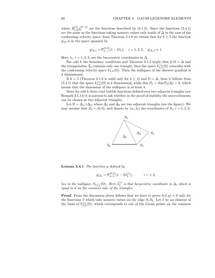
60 CHAPTER 3. GAUSS-LEGENDRE ELEMENTS
where B(3)c,∆q
(k−3)i are the functions described by (3.1.5). Since the functions (3.4.1)
are the same as the functions taking nonzero values only inside of ∆ in the case of theconforming velocity space, from Theorem 2.1.8 we obtain that for k ≥ 5 the functionq|∆ is in the space spanned by
q|∆,i = P(0,2)k−1 (1 − 2λi), i = 1, 2, 3, q|∆,4 ≡ 1.
Here λi, i = 1, 2, 3, are the barycentric coordinates in ∆.For odd k the boundary conditions and Theorem 3.1.2 imply that if Ω = ∆ and
the triangulation Th contains only one triangle, then the space V nch,k(Ω) coincides with
the conforming velocity space Vh,k(Ω). Then the nullspace of the discrete gradient is4 dimensional.
If k = 3 (Theorem 2.1.8 is valid only for k ≥ 4) and Ω = ∆, then it follows from(3.4.1) that the space V nc
h,k(Ω) is 2 dimensional, while dimPh = dim P2(∆) = 6, whichmeans that the dimension of the nullspace is at least 4.
Since for odd k there exist bubble functions defined over two adjacent triangles (seeRemark 3.1.14) it is natural to ask whether in the proof of stability the macroelementscan be chosen as two adjacent triangles.
Let Ω = ∆1∪∆2, where ∆1 and ∆2 are two adjacent triangles (see the figure). Wemay assume that S0 = (0, 0), and denote by (ai, bi) the coordinates of Si, i = 1, 2, 3.
∆1
∆2
S0 S1
S3
S2
Lemma 3.4.1 The function q defined by
q|∆i= P
(0,2)k−1 (1 − 2λ
(i)3 ), i = 1, 2,
lies in the nullspace NV nch,k
(Ω). Here λ(i)3 is that barycentric coordinate in ∆i which is
equal to 0 on the common side of the triangles.
Proof. From the discussion above follows that we have to prove b(~v, q) = 0 only forthe functions ~v which take nonzero values on the edge S1S2. Let ~v be an element ofthe basis of V nc
h,k(Ω), which corresponds to one of the Gauss points on the common
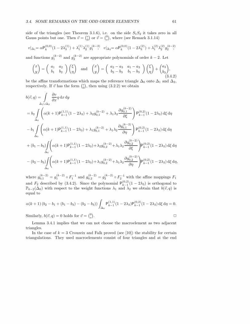
3.4. SOME REMARKS ON THE ODD ORDER ELEMENTS 61
side of the triangles (see Theorem 3.1.6), i.e. on the side S1S2 it takes zero in allGauss points but one. Then ~v =
(
v0
)
or ~v =(
0v
)
, where (see Remark 3.1.14)
v|∆1= αP
(0,0)k (1 − 2λ
(1)3 ) + λ
(1)1 λ
(1)2 g
(k−2)1 , v|∆2
= αP(0,0)k (1 − 2λ
(2)3 ) + λ
(2)1 λ
(2)2 g
(k−2)2 ,
and functions g(k−2)1 and g
(k−2)2 are appropriate polynomials of order k − 2. Let
(
x
y
)
=
(
a1 a2
b1 b2
)(
ξ
η
)
and
(
x
y
)
=
(
a2 − a3 a1 − a3
b2 − b3 b1 − b3
)(
ξ
η
)
+
(
a3
b3
)
,
(3.4.2)be the affine transformations which maps the reference triangle ∆0 onto ∆1 and ∆2,respectively. If ~v has the form
(
v0
)
, then using (3.2.2) we obtain
b(~v, q) =
∫
∆1∪∆2
∂v
∂xq dx dy
= b2
∫
∆0
(
α(k + 1)P(1,1)k−1 (1 − 2λ3) + λ2g
(k−2)0,1 + λ1λ2
∂g(k−2)0,1
∂ξ
)
P(0,2)k−1 (1 − 2λ3) dξ dη
− b1
∫
∆0
(
α(k + 1)P(1,1)k−1 (1 − 2λ3) + λ1g
(k−2)0,1 + λ1λ2
∂g(k−2)0,1
∂η
)
P(0,2)k−1 (1 − 2λ3) dξ dη
+ (b1 − b3)
∫
∆0
(
α(k + 1)P(1,1)k−1 (1 − 2λ3)+λ2g
(k−2)0,2 +λ1λ2
∂g(k−2)0,2
∂ξ
)
P(0,2)k−1 (1 − 2λ3) dξ dη
− (b2 − b3)
∫
∆0
(
α(k + 1)P(1,1)k−1 (1 − 2λ3)+λ1g
(k−2)0,2 +λ1λ2
∂g(k−2)0,2
∂η
)
P(0,2)k−1 (1 − 2λ3) dξ dη,
where g(k−2)0,1 = g
(k−2)1 F−1
1 and g(k−2)0,2 = g
(k−2)2 F−1
2 with the affine mappings F1
and F2 described by (3.4.2). Since the polynomial P(0,2)k−1 (1 − 2λ3) is orthogonal to
Pk−2(∆0) with respect to the weight functions λ1 and λ2 we obtain that b(~v, q) isequal to
α(k + 1) (b2 − b1 + (b1 − b3) − (b2 − b3))
∫
∆0
P(1,1)k−1 (1 − 2λ3)P
(0,2)k−1 (1 − 2λ3) dξ dη = 0.
Similarly, b(~v, q) = 0 holds for ~v =(
0v
)
. 2
Lemma 3.4.1 implies that we can not choose the macroelement as two adjacenttriangles.
In the case of k = 3 Crouzeix and Falk proved (see [10]) the stability for certaintriangulations. They used macroelements consist of four triangles and at the end
62 CHAPTER 3. GAUSS-LEGENDRE ELEMENTS
of their paper they announced that they think the stability of the element for anytriangulation of a convex polygon.
Theorem 3.4.2 (See [30, 31]) For odd-order Gauss-Legendre elements there is noCrouzeix-Velte decomposition.
The spectrum of the discrete Schur complement operator in the case of the first-order Crouzeix-Raviart element (see in Section 1.6) on the unit square using a stan-dard triangulation is shown in Chapter 4. In this case the eigenvalues are in [0, 2):the Crouzeix-Velte decomposition does not exist.
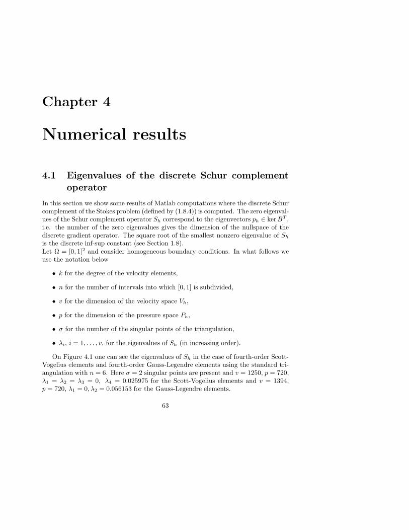
Chapter 4
Numerical results
4.1 Eigenvalues of the discrete Schur complement
operator
In this section we show some results of Matlab computations where the discrete Schurcomplement of the Stokes problem (defined by (1.8.4)) is computed. The zero eigenval-ues of the Schur complement operator Sh correspond to the eigenvectors ph ∈ kerBT ,i.e. the number of the zero eigenvalues gives the dimension of the nullspace of thediscrete gradient operator. The square root of the smallest nonzero eigenvalue of Sh
is the discrete inf-sup constant (see Section 1.8).Let Ω = [0, 1]2 and consider homogeneous boundary conditions. In what follows weuse the notation below
• k for the degree of the velocity elements,
• n for the number of intervals into which [0, 1] is subdivided,
• v for the dimension of the velocity space Vh,
• p for the dimension of the pressure space Ph,
• σ for the number of the singular points of the triangulation,
• λi, i = 1, . . . , v, for the eigenvalues of Sh (in increasing order).
On Figure 4.1 one can see the eigenvalues of Sh in the case of fourth-order Scott-Vogelius elements and fourth-order Gauss-Legendre elements using the standard tri-angulation with n = 6. Here σ = 2 singular points are present and v = 1250, p = 720,λ1 = λ2 = λ3 = 0, λ4 = 0.025975 for the Scott-Vogelius elements and v = 1394,p = 720, λ1 = 0, λ2 = 0.056153 for the Gauss-Legendre elements.
63

64 CHAPTER 4. NUMERICAL RESULTS
0 100 200 300 400 500 600 700 8000
0.2
0.4
0.6
0.8
1
n=6, standard grid: Scott−Vogelius (dashed) and Gauss−Legendre (solid)
Figure 4.1: Eigenvalues of Sh on the standard triangulation of the unit square, n=6. Lowercurve: P
24 − P3 (Scott-Vogelius element), here λ1 = λ2 = λ3 = 0, λ4 = 0.025975, upper
curve: (P4 + B(4)n )2 − P3 (Gauss-Legendre element): λ2 = 0.056153.
0 200 400 600 800 1000 1200 14000
0.2
0.4
0.6
0.8
1
n=6, criss−cross grid: Scott−Vogelius (dashed) and Gauss−Legendre (solid)
Figure 4.2: Eigenvalues of Sh on the criss-cross triangulation of the unit square, n=6. Lowercurve: P
24 − P3 (Scott-Vogelius element), here λ1 = . . . = λ37 = 0, λ38 = 0.179739, upper
curve: (P4 + B(4)n )2 − P3 (Gauss-Legendre element): λ2 = 0.212876
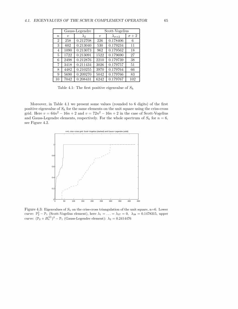
4.1. EIGENVALUES OF THE SCHUR COMPLEMENT OPERATOR 65
Gauss-Legendre Scott-Vogeliusn v λ2 v λσ+2 σ + 22 258 0.212708 226 0.178406 63 602 0.213040 530 0.179234 114 1090 0.213073 962 0.179562 185 1722 0.213091 1522 0.179690 276 2498 0.212876 2210 0.179739 387 3418 0.211434 3026 0.179757 518 4482 0.210255 3970 0.179764 669 5690 0.209270 5042 0.179766 83
10 7042 0.208431 6242 0.179767 102
Table 4.1: The first positive eigenvalue of Sh
Moreover, in Table 4.1 we present some values (rounded to 6 digits) of the firstpositive eigenvalue of Sh for the same elements on the unit square using the criss-crossgrid. Here v = 64n2 − 16n + 2 and v = 72n2 − 16n + 2 in the case of Scott-Vogeliusand Gauss-Legendre elements, respectively. For the whole spectrum of Sh for n = 6,see Figure 4.2.
0 50 100 150 200 250 300 350 400 4500
0.2
0.4
0.6
0.8
1
n=6, criss−cross grid: Scott−Vogelius (dashed) and Gauss−Legendre (solid)
Figure 4.3: Eigenvalues of Sh on the criss-cross triangulation of the unit square, n=6. Lowercurve: P
22 − P1 (Scott-Vogelius element), here λ1 = . . . = λ37 = 0, λ38 = 0.1478315, upper
curve: (P2 + B(2)n )2 − P1 (Gauss-Legendre element): λ2 = 0.2414476
66 CHAPTER 4. NUMERICAL RESULTS
In the case of the second order Scott-Vogelius and Gauss-Legendre (i.e. Fortin-Soulie) elements the eigenvalues of Sh can be seen on Figure 4.3. Here we used thecriss-cross triangulation of the unit square for n = 6. Then σ = 36 and v = 530,p = 432 in the conforming case, while v = 818, p = 432 in the non-conformingcase. In all of the previous cases the eigenvalues lie in the [0, 1] interval which is aconsequence of the existence of the Crouzeix-Velte decomposition (see Section 1.8).
Figure 4.4 shows the spectrum of the first-order Crouzeix-Raviart element (seeSection 1.6) on the unit square using the standard triangulation with n = 20. Inthis case v = 2n(3n − 2) = 2320, while p = 2n2 = 800. The first nonzero eigenvalueis equal to 0.270649 and the eigenvalues are in [0, 2), so the element does not haveCrouzeix-Velte decomposition (see [31]).
0 100 200 300 400 500 600 700 8000
0.2
0.4
0.6
0.8
1
1.2
1.4
1.6
1.8
2Crouzeix−Raviart element, n=20
Figure 4.4: Eigenvalues of Sh in the case of first order Crouzeix-Raviart element.
4.2 Solution of a test problem
Let Ω = [0, 1]2 and consider the Stokes equations in the case of
u(x, y) = (sin x sin y, cosx cos y)T ,
p(x, y) = 2 cosx sin x − 2 sin(1)(1 − cos(1)),
f(x, y) = (0, 4 cosx cos y)T .
This problem is described in [4] and also investigated in [18].

4.2. SOLUTION OF A TEST PROBLEM 67
For the solution of the Stokes equations we used the criss-cross triangulation of theunit square and fourth-order Gauss-Legendre and Scott-Vogelius elements. Numericalcalculations were performed using Matlab.
We solved the linear equation by Uzawa algorithm with conjugate directions (see[3, Chapter IV]).
In Tables 4.2 and 4.3 we present the number of iteration steps and the errors ofthe discrete velocity and pressure, where the norm || · ||(0,h) is defined on R
N as
||x||2(0,h) := h2N∑
i=1
x2i , x = (x1, . . . , xN )T ,
and h = 1/n.
n ||uh − u||(0,h) ||ph − p||(0,h) steps2 1.82630613 · 10−6 2.459486 · 10−2 764 7.37690783 · 10−8 5.930648 · 10−3 978 3.83938455 · 10−9 1.145399 · 10−3 98
16 2.26807489 · 10−10 3.598438 · 10−4 9832 1.38766900 · 10−11 8.950061 · 10−5 99
Table 4.2: Gauss-Legendre elements.
n ||uh − u||(0,h) ||ph − p||(0,h) steps2 1.30900265 · 10−6 2.459450 · 10−2 924 4.14507706 · 10−8 5.930621 · 10−3 1108 1.30255577 · 10−9 1.145398 · 10−3 119
16 4.08131908 · 10−11 3.598437 · 10−4 12132 1.28732502 · 10−12 8.950061 · 10−5 122
Table 4.3: Scott-Vogelius elements.

68 CHAPTER 4. NUMERICAL RESULTS
Summary
In the present work we deal with a high-order non-conforming finite element familyfor the two dimensional Stokes equations.
Let ~viNi=1 and qiM
i=1 be bases of the given finite element spaces Vh (velocities)and Ph (pressures), respectively. The matrix form of the discrete Stokes equations is
(
Ah BTh
Bh 0
)(
up
)
=
(
fh
0
)
,
where
Ah := (aij)Ni,j=1, aij := a(~vi, ~vj),
Bh := (bij)N,Mi,j=1, bij := b(~vj , qi),
fh := (fi)Ni=1, fi := (~f,~vi)0,
~uh :=
N∑
i=1
yi~vi, ph :=
M∑
i=1
ziqi,
u := (y1, . . . , yN)T , p := (z1, . . . , zM )T ,
and the bilinear functionals a(·, ·) and b(·, ·) are defined as
a(~u,~v) :=∑
∆∈Th
∫
∆
2∑
i=1
2∑
j=1
∂ui
∂xj
∂vi
∂xjdx,
b(~v, p) := −∑
∆∈Th
∫
∆
p div~v dx.
To prove stability of the finite element pair (Vh, Ph) we have to check the inf-supcondition
sup~vh∈Vh
b(~vh, qh)
|~v|1≥ βh inf
q0h∈kerBTh
||qh + q0h||L2(Ω) = βh||qh||L2(Ω)/ ker BTh
∀qh ∈ Ph,
where βh ≥ β0 > 0 with a constant β0 independent of h.
69

70 SUMMARY
First we investigate the Scott-Vogelius finite element family where velocities andpressures are approximated trianglewise by polynomials of order k and (k − 1), re-spectively. Moreover, the discrete velocities are assumed to be continuous, but thereis no continuity requirement on the pressure:
Ph(Ω) :=
p ∈ L2(Ω) : p|∆ ∈ Pk−1(∆), ∆ ∈ Th
, (5.1.1)
Vh,k(Ω) :=
~v ∈ (H10 (Ω))2 : ~v|∆ ∈ (Pk(∆))2, ∆ ∈ Th
. (5.1.2)
For k ≥ 4 Scott and Vogelius [24] proved the stability of the finite element pair(2.1.1)–(2.1.2) under a condition connected with the grid singularity. A vertex of thetriangulation is called a singular point if the edges meeting at this vertex lie on twostraight lines. In [24] the authors showed that in the case of k ≥ 4 if the number ofthe singular points in the triangulation is equal to σ then the nullspace of the discretegradient operator is σ + 1 dimensional. Moreover, for k ≥ 4 the finite element pair(2.1.1)–(2.1.2) is inf-sup stable if the triangulation does not contain near-singularpoints. In the case when near-singular points approach singular points, the rightinverse of the divergence operator is blowing up.
The aim of the present dissertation is to describe a finite element family that is –similarly to the Scott-Vogelius elements – defined for arbitrary order k, moreover itis inf-sup stable without a restriction on the grid.
In Chapter 2 we investigate the nullspace of the discrete gradient operator in thecase of the Scott-Vogelius elements (in [25] just the dimension of this space is given).We show that if the triangulation of a polygonal domain Ω contains σ singular points,then for k ≥ 4 there exists a basis of the nullspace which can be given in the followingway. Besides the constant function, to each singular point corresponds a functionwhich is zero everywhere except on the triangles around the given point.
In the description of the basis we use orthogonal polynomials defined on triangles(see in [17]).
At the end of this chapter we give some examples where in the case of k = 2, 3the dimension of the nullspace can be greater as σ + 1.
In Chapter 3 we define the Gauss-Legendre finite element family for arbitraryorder k. In this case the velocities are assumed to be continuous on the common sideof two adjacent triangles only in certain points that are the roots of the kth-orderLegendre polynomial given on this side. The discrete spaces are
Ph(Ω) :=
p ∈ L2(Ω), p|∆ ∈ Pk−1(∆), ∆ ∈ Th
, (5.1.3)
V nch,k(Ω) :=
~v ∈ (L2(Ω))2, ~v|∆ ∈ (Pk(∆))2, and ~v is continuous in all
kth-order Gauss-Legendre points of all sides of ∆, ∆ ∈ Th, ~v = 0 in
all kth-order Gauss-Leg. points on the triangle sides E ⊂ Γ , (5.1.4)
SUMMARY 71
while the norm in V nch,k(Ω) is defined as
|~vh|1,h,Ω :=
(
∑
∆∈Th
|~vh|21,∆
)1/2
.
Since V nch,k(Ω) 6⊂ (H1(Ω))2, the approximation is non-conforming.
In Subsection 3.1 we specify suitable degrees of freedom for the velocity parts ofthese elements. Let ∆ be a given triangle and consider the kth-order Gauss-Legendre
points on the sides of ∆ together with the (k−2)(k−1)2 inner points having barycentric
coordinates
λ1 =j
k, λ2 =
ℓ
k, λ3 =
m
k, 1 ≤ j, ℓ, m ≤ k − 2, j + ℓ + m = k.
The nullspace of the interpolation problem of finding a kth-order polynomial whichtakes prescribed values in these points is trivial if k is odd and one-dimensional if kis even. For odd values of k we can use the points above as degrees of freedom, whilefor even k there exist (“bubble”-) functions which take zero values in the kth-orderGauss-Legendre points.
On the triangle ∆ we define the kth-order non-conforming bubble function as
B(k)n,∆ :=
1
2
3∑
i=1
P(0,0)k (1 − 2λi) − 1
.
For odd k it is equal to zero on the sides of ∆, while for even k one gets the non-conforming velocity space V nc
h,k(Ω) by adding trianglewise a kth-order non-conformingbubble function to the conforming velocity space Vh,k(Ω), that is
V nch,k(Ω) = Vh,k(Ω) +
~v, ~v|∆ =
(
α∆
β∆
)
B(k)n,∆, α∆, β∆ ∈ R, ∆ ∈ Th
.
In Chapter 3 for even k we prove the stability of (5.1.3)–(5.1.4) using a modification ofthe macroelement technique of Stenberg [26]. We define finitely many macroelementclasses satisfying
(i) for each macroelement M from the classes the nullspace of the discrete gradientoperator defined over M is one-dimensional, consisting of functions that areconstant on M , i.e. dim Nnc
M = 1, where
NncM =
p ∈ PM :
∫
M
p div~v dx = 0 ∀~v ∈ V nc0,M
,
V nc0,M =
~v : ~v|∆ ∈ (Pk(∆))2 ∀∆ ∈ M, and ~v is continuous in all
kth-order Gauss-Legendre points of all sides of ∆, ∆ ⊂ M, ~v = 0 in all
kth-order Gauss-Legendre points of all edges on ∂M ,

72 SUMMARY
(ii) for each h the triangles in Th can be grouped to form macroelements such thatfor the so obtained macroelement partitioning each macroelement belongs toone of the macroelement classes.
If the above macroelement conditions are satisfied then for k ≥ 2 the inf-sup conditionholds for the finite element family defined in (5.1.3)–(5.1.4).
An important step in the proof of stability is the study of the nullspace. In Section3.2 we prove that for even k by adding trianglewise a non-conforming bubble functionto the space Vh,k(Ω) the nullspace of the discrete gradient operator becomes one-dimensional. In the proof we use that the basis of the nullspace in the conformingcase has already been described in Subsection 2.1.2.
Since in the case of even k the nullspace NV nch,k
(Ω) is one-dimensional for arbitrarypolygonal domains Ω the only restriction in the choice of the macroelement classes isthe macroelement condition (ii). The simplest possibility is to define only one class,such that each macroelement from this class consists of a single triangle.
In Chapter 4 we give some numerical results where for different values of k and forvarious triangulations in the case of Scott-Vogelius and Gauss-Legendre elements wecompute the discrete inf-sup constants. Further, using fourth-order Gauss-Legendreelements we solve a test equation described in [4].
Osszefoglalo
A dolgozat a ket-dimenzios Stokes feladat numerikus megoldasa kapcsan egy magasrendu nemkonform vegeselem csalad vizsgalataval foglalkozik.
A Stokes feladat egy osszenyomhatatlan, viszkozus folyadek lassu aramlasat leıroegyenletrendszer:
−~∆~u + gradp = ~f, (6.1.1)
−div ~u = 0, (6.1.2)
~u|Γ = ~u0, (6.1.3)
ahol Ω egy ket-dimenzios tartomany Lipschitz folytonos hatarral (Ω peremet jeloli Γ),
~u : Ω → R2 es p : Ω → R a keresett sebesseg, illetve nyomas, ~f adott kulso ero.
Az egyenletekbol a nyomas csak egy additıv konstantol eltekintve hatarozhato megegyertelmuen, adott p eseten a sebesseg vektor egyertelmu.
A feladatnak homogen peremfeltetelek eseten a numerikus megoldashoz hasznosvariacos megfogalmazasa a kovetkezo. Olyan ~u ∈ (H1
0 (Ω)2 es p ∈ L20(Ω) fuggvenyeket
keresunk, melyek kielegıtik az alabbi egyenleteket:
a(~u,~v)+b(~v, p) = (~f,~v)0 ∀~v ∈ (H10 (Ω))2, (6.1.4)
b(~u, q) = 0 ∀q ∈ L20(Ω). (6.1.5)
Az a(·, ·) es b(·, ·) bilinearis funkcionalok ertelmezese
a(~u,~v) :=
∫
Ω
2∑
i=1
2∑
j=1
∂ui
∂xj
∂vi
∂xjdx, (6.1.6)
b(~v, p) := −
∫
Ω
p div~v dx. (6.1.7)
Hasonloan (6.1.4)–(6.1.5) tıpusu egyenletekre vezet peldaul a stacionarius hovezetestleıro egyenletrendszer.
A (6.1.4)–(6.1.5) feladat egyertelmuen megoldhato, mert az a(·, ·) funkcional el-liptikus es teljesul az ugy nevezett inf-sup feltetel: letezik olyan β konstans, hogy
infp∈L2
0(Ω)sup
~v∈(H10 (Ω))2
b(v, p)
|~v|1 · ||p||0≥ β > 0,
73

74 OSSZEFOGLALO
ahol |~v|21 = a(~v,~v).A (6.1.4)–(6.1.5) vegeselem diszkretizaciojahoz az Ω (poligonalis) tartomanyt ha-
romszogekre osztjuk, a keresett sebesseget es nyomast haromszogenkent adott foksza-mu polinomokkal kozelıtjuk.
Egy – a dolgozatban reszletesebben is vizsgalt – vegeselem csalad a Scott-Vogeliuselemek. Itt a sebesseget haromszogenkent k-ad, a nyomast haromszogenkent k − 1-edrendu polinomokkal kozelıtjuk, a sebesseg eseten feltetelezzuk, hogy a polinomoka szomszedos haromszogek kozos oldalan folytonosak, mıg a nyomast kozelıto poli-nomok eseten nincs ilyen feltetel. A vegeselem par tetszoleges k ≥ 1 egesz esetendefinialt. A legfeljebb k-adfoku polinomok teret Pk-val jelolve az Ω tartomany egy Th
triangularizacioja eseten a (H10 (Ω))2 es az L2(Ω) tereket approximalo Vh es Ph terek
a kovetkezok:
Vh = Vh,k(Ω) =
~v ∈ (H10 (Ω))2 : ~v|∆ ∈ (Pk(∆))2, ∆ ∈ Th
, (6.1.8)
Ph(Ω) =
p ∈ L2(Ω) : p|∆ ∈ Pk−1(∆), ∆ ∈ Th
. (6.1.9)
Ha – mint a fenti esetben – a Vh, ill. Ph ter resze annak a ternek, ahol az ere-deti (6.1.4)–(6.1.5) problemat megfogalmaztuk (jelen esetben a (H1
0 (Ω))2, ill. L2(Ω)ternek), akkor konform approximaciorol beszelunk. Ekkor a diszkret variacios feladat:olyan ~uh ∈ Vh es ph ∈ Ph fuggvenyeket keresunk, melyekre
a(~uh, ~vh)+b(~vh, ph) = (~f,~vh)0 ∀~vh ∈ Vh, (6.1.10)
b(~uh, qh) = 0 ∀qh ∈ Ph ∩ L20(Ω) (6.1.11)
teljesul. Ha ~viNi=1 es qiM
i=1 a Vh, illetve Ph terek bazisai, akkor a diszkret feladatmatrix alakja
(
Ah BTh
Bh 0
)(
up
)
=
(
fh
0
)
,
ahol
Ah := (aij)Ni,j=1, aij := a(~vi, ~vj),
Bh := (bij)N,Mi,j=1, bij := b(~vj , qi),
fh := (fi)Ni=1, fi := (~f,~vi)0,
~uh :=
N∑
i=1
yi~vi, ph :=
M∑
i=1
ziqi,
u := (y1, . . . , yN )T , p := (z1, . . . , zM )T .
A (6.1.10)–(6.1.11) feladat egyertelmuen megoldhato es a megoldas stabil, haletezik olyan βh > 0 konstans, hogy
sup~vh∈Vh
b(~vh, qh)
|~v|1≥ βh inf
q0h∈kerBTh
||qh + q0h||L2(Ω) = βh||qh||L2(Ω)/ ker BTh
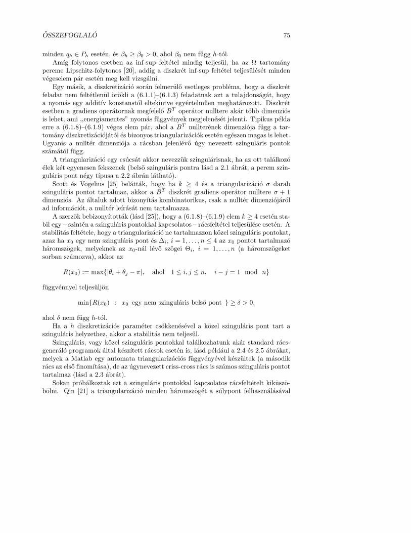
OSSZEFOGLALO 75
minden qh ∈ Ph eseten, es βh ≥ β0 > 0, ahol β0 nem fugg h-tol.Amıg folytonos esetben az inf-sup feltetel mindig teljesul, ha az Ω tartomany
pereme Lipschitz-folytonos [20], addig a diszkret inf-sup feltetel teljesuleset mindenvegeselem par eseten meg kell vizsgalni.
Egy masik, a diszkretizacio soran felmerulo esetleges problema, hogy a diszkretfeladat nem feltetlenul orokli a (6.1.1)–(6.1.3) feladatnak azt a tulajdonsagat, hogya nyomas egy additıv konstanstol eltekintve egyertelmuen meghatarozott. Diszkretesetben a gradiens operatornak megfelelo BT operator nulltere akar tobb dimenziosis lehet, ami ,,energiamentes” nyomas fuggvenyek megjeleneset jelenti. Tipikus peldaerre a (6.1.8)–(6.1.9) veges elem par, ahol a BT nullterenek dimenzioja fugg a tar-tomany diszkretizaciojatol es bizonyos triangularizaciok eseten egeszen magas is lehet.Ugyanis a nullter dimenzioja a racsban jelenlevo ugy nevezett szingularis pontokszamatol fugg.
A triangularizacio egy csucsat akkor nevezzuk szingularisnak, ha az ott talalkozoelek ket egyenesen fekszenek (belso szingularis pontra lasd a 2.1 abrat, a perem szin-gularis pont negy tıpusa a 2.2 abran lathato).
Scott es Vogelius [25] belattak, hogy ha k ≥ 4 es a triangularizacio σ darabszingularis pontot tartalmaz, akkor a BT diszkret gradiens operator nulltere σ + 1dimenzios. Az altaluk adott bizonyıtas kombinatorikus, csak a nullter dimenziojarolad informaciot, a nullter leırasat nem tartalmazza.
A szerzok bebizonyıtottak (lasd [25]), hogy a (6.1.8)–(6.1.9) elem k ≥ 4 eseten sta-bil egy – szinten a szingularis pontokkal kapcsolatos – racsfeltetel teljesulese eseten. Astabilitas feltetele, hogy a triangularizacio ne tartalmazzon kozel szingularis pontokat,azaz ha x0 egy nem szingularis pont es ∆i, i = 1, . . . , n ≤ 4 az x0 pontot tartalmazoharomszogek, melyeknek az x0-nal levo szogei Θi, i = 1, . . . , n (a haromszogeketsorban szamozva), akkor az
R(x0) := max|θi + θj − π|, ahol 1 ≤ i, j ≤ n, i − j = 1 mod n
fuggvennyel teljesuljon
minR(x0) : x0 egy nem szingularis belso pont ≥ δ > 0,
ahol δ nem fugg h-tol.Ha a h diszkretizacios parameter csokkenesevel a kozel szingularis pont tart a
szingularis helyzethez, akkor a stabilitas nem teljesul.Szingularis, vagy kozel szingularis pontokkal talalkozhatunk akar standard racs-
generalo programok altal keszıtett racsok eseten is, lasd peldaul a 2.4 es 2.5 abrakat,melyek a Matlab egy automata triangularizacios fuggvenyevel keszultek (a masodikracs az elso finomıtasa), de az ugynevezett criss-cross racs is szamos szingularis pontottartalmaz (lasd a 2.3 abrat).
Sokan probalkoztak ezt a szingularis pontokkal kapcsolatos racsfeltetelt kikuszo-bolni. Qin [21] a triangularizacio minden haromszoget a sulypont felhasznalasaval

76 OSSZEFOGLALO
harom kisebb haromszogre bontotta es az ıgy kapott makroelemeken definialt poli-nomokkal kozelıtette a megoldast.
Tobb munka kiindulopontja a Fortin es Soulie [13] altal definialt masodrenduvegeselem par volt. A szerzok ott a Vh = Vh,2 ter bovıtesevel biztosıtottak a szingularispontoktol fuggetlen stabilitast, az altaluk definialt vegeselem par:
Ph(Ω) = p ∈ L2(Ω), p|∆ ∈ P1(∆), ∆ ∈ Th (6.1.12)
V nch,2(Ω) =
~v ∈ (L2(Ω))2, ~v|∆ ∈ (P2(∆))2, es ~v folytonos ket szomszedos
haromszog kozos oldalan a masodrendu Gauss-Legendre pontokban,
~v = 0 a Γ-n fekvo oldalak msodrendu Gauss-Legendre pontjaiban .(6.1.13)
Itt tehat a diszkret sebessegek folytonossagat ket szomszedos haromszog kozos oldalancsak bizonyos pontokban koveteljuk meg: a masodfoku Legendre polinom zerushelye-in. Ekkor a V nc
h,2 ter nem resze a (H1(Ω))2 ternek, a veges elem nem konform. Ebbenaz esetben az a(·, ·) es b(·, ·) funkcionalokat a kovetkezo modon definialjuk:
a(~u,~v) :=∑
∆∈Th
∫
∆
2∑
i=1
2∑
j=1
∂ui
∂xj
∂vi
∂xjdx, (6.1.14)
b(~v, p) := −∑
∆∈Th
∫
∆
p div~v dx, (6.1.15)
mıg a | · |1,h szemi-norma
|~v|1,h :=√
a(~v,~v). (6.1.16)
A V nch,2(Ω) ter a Vh,2 konform terbol szarmaztathato oly modon, hogy a Vh,2 ter lokalis
bazisahoz haromszogenkent hozzaadunk egy masodfoku polinomot (egy ugy nevezettbuborek fuggvenyt), amely a haromszog oldalain a masodrendu Gauss-Legendre pon-tokban eltunik:
V nch,2(Ω) = Vh,2(Ω) +
~v, ~v|∆ =
(
α∆
β∆
)
b∆, α∆, β∆ ∈ R, ∆ ∈ Th
,
ahol λi-vel, i = 1, 2, 3, jelolve a ∆ haromszogben a baricentrikus koordinatakat
b∆ := 3(λ21 + λ2
2 + λ23) − 2.
Matthies es Tobiska [18] egy tetszoleges k rend eseten definialt nemkonform elemcsaladot ırt le, de a szerzok a k-adrendu konform teret haromszogenkent egy k + 1-edfoku buborek fuggvennyel bovıtettek. Az ıgy kapott veges elem a racs szingu-laritasatol fuggetlenul stabil.
Y. Cha, M. Lee es S. Lee [7] a k = 4, 6 esetet vizsgalta, itt a konform terhez adottbuborek fuggveny fokszama 4, ill. 6, de a stabilitas bizonyıtasahoz a b(·, ·) bilinearis

OSSZEFOGLALO 77
format egy stabilizalo taggal egeszıtettek ki, amely egy alkalmasan megvalasztottparametert tartalmaz.
Jelen dolgozat temaja egy nemkonform vegeselem csalad leırasa, mely tetszolegesk rend eseten definialt es paros k eseten a racs szingularitasatol fuggetlenul stabil.
A (6.1.12)–(6.1.13) elemhez hasonloan a k-adrendu Gauss-Legendre elemet a ko-vetkezo modon definialjuk:
Ph(Ω) = p ∈ L2(Ω), p|∆ ∈ Pk−1(∆), ∆ ∈ Th (6.1.17)
V nch,k(Ω) =
~v ∈ (L2(Ω))2, ~v|∆ ∈ (Pk(∆))2, es ~v folytonos ket szomszedos
haromszog kozos oldalan a k-adrendu Gauss-Legendre pontokban,
~v = 0 a Γ-n fekvo oldalak k-adrendu Gauss-Legendre pontjaiban .(6.1.18)
Ez a csalad jol ismert alacsony rendu veges elemek altalanosıtasa, k = 1, k = 2,k = 3 eseten (6.1.17)–(6.1.18) rendre a Crouzeix-Raviart [11], Fortin-Soulie [13] esCrouzeix-Falk [10] elemeket definialja.
Az a(·, ·) es b(·, ·) bilinearis formakat es a | · |1,h szemi-normat itt is az (6.1.14)–(6.1.16) kepletekkel ertelmezzuk. Mivel a sebessegek folytonossagat ket szomszedosharomszog kozos oldalan a k-adrendu Gauss-Legendre pontokban koveteljuk meg, azugy nevezett ,,patch-feltetel” teljesul es (6.1.16) normat definial V nc
h,k(Ω)-n [11].A Gauss-Legendre elemek vizsgalataval a dolgozat 3. fejezete foglalkozik. A 3.1
alfejezetben az elem reszletes leırasa szerepel, itt eloszor a V nch,k szabadsagi fokait
vizsgaljuk. Egy adott ∆ haromszog eseten tekintsuk a haromszog oldalain a k-adrenduGauss-Legendre pontokat, a haromszog belsejeben pedig a
λ1 =j
k, λ2 =
ℓ
k, λ3 =
m
k, 1 ≤ j, ℓ, m ≤ k − 2, j + ℓ + m = k,
baricetrikus koordinatakkal leırt pontokat. Ha olyan p ∈ Pk(∆) polinomot keresunk,
mely az ıgy definialt 3k + (k−2)(k−1)2 = (k+1)(k+2)
2 darab pontban megadott ertekeketvesz fel, a keletkezo interpolacios feladat nulltere trivialis, ha k paratlan es egy-dimenzios, ha k paros. Ezek alapjan paratlan k eseten a fenti pontokat valaszthatjukszabadsagi fokoknak, paros k eseten viszont letezik olyan, az adott haromszog folottdefinialt k-adfoku polinom, amely a haromszog peremen a k-adrendu Legendre pon-tokban eltunik. A k-adrendu nemkonform buborek fuggvenyt tetszoleges paros kesetere a kovetkezo alakban definialtuk:
B(k)n,∆ :=
1
2
3∑
i=1
P(0,0)k (1 − 2λi) − 1
, (6.1.19)
ahol P(0,0)k jeloli a k-adfoku, [−1, 1]-en definialt 1 foegyutthatoju Legendre polinomot.
k = 2 eseten ez a Fortin es Soulie altal definialt masodrendu b∆ buborek fuggvennyelegyenlo, mıg k = 4 es k = 6 eseten a Y. Cha, M. Lee es S. Lee [7] altal hasznalt buborek

78 OSSZEFOGLALO
fuggvenyektol csak egy konform (a haromszog minden oldalan eltuno) buborek tagbankulonbozik.
Belattuk, hogy paratlan k eseten ha egy polinom erteke a k-adrendu Gauss-Legendre pontokban nulla, akkor a polinom a haromszog teljes peremen eltunik.
Paros rendu elemek eseten (hasonloan a masodrendu elemhez) a V nch,k(Ω) teret a
konform Vh,k ter alabbi bovıtesekent is ertelmezhetjuk:
V nch,k(Ω) = Vh,k(Ω) +
~v, ~v|∆ =
(
α∆
β∆
)
B(k)n,∆, α∆, β∆ ∈ R, ∆ ∈ Th
.
A (6.1.17)–(6.1.18) elem stabilitasat paros k eseten bizonyıtottuk, ehhez a 3.3 alfe-jezetben a konform elemekre alkalmazhato Stenberg-fele makroelem modszert (lasd[26]) modosıtottuk nemkonform elemek esetere. A modszer lenyege, hogy veges sokolyan makroelem osztalyt definialunk, hogy
(i) az osztalyok mindegyikere teljesul, hogy az abba tartozo M makroelemek folotta diszkret gradiens operator nulltere egy-dimenzios (csak a konstans fuggvenye-ket tartalmazza), azaz dim Nnc
M = 1, ahol
NncM =
p ∈ Ph :
∫
M
p div~v dx = 0 ∀~v ∈ V nc0,M
,
V nc0,M =
~v : ~v|∆ ∈ (Pk(∆))2 ∀∆ ∈ M, es ~v folytonos minden k-adrendu
Gauss-Legendre pontban ket szomszedos haromszog kozos oldalan,
~v = 0 a k-adrendu Gauss-Leg. pontokban a ∂M -hez tartozo oldalakon ,
(ii) tetszoleges h eseten a triangularizacio haromszogei osszecsoportosıthatoak mak-roelemekke ugy, hogy a makroelemek egyertelmuen osztalyba sorolhatoak.
Ha a fenti ket makroelem feltetel teljesul, akkor a veges elem inf-sup stabil.A stabilitasi bizonyıtas egy lenyeges eleme a nullter vizsgalata, amihez elobb a
2.1.2 alfejezetben leırtuk a nullteret a konform Scott-Vogelius elem eseten mindenk ≥ 4-re. Itt felhasznalva Scott es Vogelius allıtasat a nullter dimenziojarol tetszolegesk ≥ 4 eseten megadtuk a nullter egy bazisat. Ha σ jeloli a szingularis pontok szamat,akkor a bazis a konstans fuggvenyen kıvul σ darab olyan fuggvenyt tartalmaz, melyekmindegyike megfeleltetheto valamelyik szingularis pontnak: csak a pontot tartalmazoharomszogekben vesz fel nullatol kulonbozo ertekeket.
A bazis leırasahoz haromszogek folott definialt ortogonalis polinomokat hasznal-tunk (lasd [17]), alapveto szerepet jatszott a (0, 2) parameteru (k−1)-edrendu Jacobi-polinom.
A 2.1.2 alfejezet vegen nehany peldaval szemleltettuk, hogy a Scott-Vogelius ele-mek eseten ha k = 2, 3 a nullter dimenzioja nagyobb is lehet, mint σ + 1.
OSSZEFOGLALO 79
A 3.2 alfejezetben – felhasznalva a 2.1.2 alfejezetben leırt bazist – megmutattuk,hogy paros k ≥ 4 eseten a nemkonform buborek fuggvennyel bovıtve a konform tereta nullter egy-dimenziossa valik. A k = 2 esetre a bizonyıtas (mivel itt a konform elem-hez tartozo nullter leırasa nem ismert) mas modszerrel a 2.2 alfejezetben talalhato.Igy belattuk, hogy tetszoleges paros k-ra a diszkret gradiens operator nulltere egy-dimenzios a triangularizaciotol es lenyegeben az Ω tartomanytol fuggetlenul, ezert astabilitasi bizonyıtasban a makroelem osztalyok definialasanal csak az (ii) makroelemfeltetel teljesulesere kell figyelnunk. A legegyszerubb eset, ha csupan egyetlen osztalytdefinialunk –az ebbe az osztalyba tartozo makroelemek egyetlen haromszogbol allnak,ıgy az (ii) feltetel trivialisan teljesul.
A paros rendu Gauss-Legendre elemek stabilitasabol k = 2 eseten kovetkezik a(6.1.12)–(6.1.13) elem stabilitasa is. Fortin es Soulie [13] munkajukban ugyan allıtjaka masodrendu elem stabilitasat, ennek bizonyıtasat azonban nem kozoltek.
A Gauss-Legendre elemek stabilitasat csak paros rend eseten sikerult bizonyıtani.Paratlan k eseten nem letezik olyan nemkonform buborek fuggveny, amely a harom-szog oldalain csak a Gauss-Legendre pontokban egyenlo nullaval – ennek a fuggveny-nek lenyeges szerepe van abban, hogy paros k eseten a diszkret gradiens operatornulltere egy-dimenzios. A 3.1 alfejezetben a paratlan k rendu Gauss-Legendre elemekleırasanal ket szomszedos (kozos oldallal rendelkezo) haromszog folott olyan k-adfokupolinomokat definialtunk, melyek a ket haromszog alkotta negyszog kulso oldalan ak-adrendu Gauss-Legendre pontokban eltunnek. Termeszetesen adodik a kerdes, hogynem lehet-e paratlan rend eseten a stabilitast ugy bizonyıtani, hogy makroelemkentket szomszedos haromszog alkotta negyszogeket valasztunk? A 3.4 alfejezetben meg-mutattuk, hogy ıgy valasztva a makroelemeket az (i) makroelem feltetel nem teljesul,a stabilitas ıgy nem bizonyıthato.
A k = 3 esetben bizonyos triangularizaciok eseten a stabilitast Crouzeix es Falk[10] bizonyıtotta, a szerzok a cikkuk vegen megjegyzik, hogy sejtesuk szerint a sta-bilitas tetszoleges racs eseten igaz.
A 4. fejezetben a nemkonform veges elemekkel kapcsolatos numerikus eredme-nyeket kozlunk. Matlab programok segıtsegevel a Scott-Vogelius es a Gauss-Legendreelemek eseten az egysegnegyzet kulonbozo triangularizacioira kiszamıtottuk a diszkretinf-sup konstanst nehany k ertekre (lasd [31]). A futasi eredmenyek alatamasztjak adiszkret gradiens nullterenek dimenziojara vonatkozo elmeleti eredmenyeket is.
Szinten Matlab segıtsegevel az egysegnegyzet criss-cross triangularizacioja esetena negyedrendu Gauss-Legendre elemet hasznalva megoldottunk egy Braess es Sarazinaltal [4] ismertetett tesztfeladatot.

80 OSSZEFOGLALO
Bibliography
[1] K. Atkinson, W. Han, Theoretical Numerical Analysis: A Functional AnalysisFramework, Springer-Verlag, New York, 2001.
[2] A. Baran, G. Stoyan, Gauss-Legendre elements: a stable, higher order non-conforming finite element family, Computing 79, 1–21 (2007).
[3] D. Braess, Finite Elements: Theory, fast solvers, and applications in solid me-chanics, Cambridge University Press, Cambridge, 1997.
[4] D. Braess, R. Sarazin, An efficient smoother for the Stokes problem, AppliedNumerical Mathematics 23, 3–19 (1997).
[5] F. Brezzi, R. S. Falk, Stability of higher-order Taylor-Hood methods, SIAMJournal on Numerical Analysis 28, 581–590 (1991).
[6] F. Brezzi, M. Fortin, Mixed and Hybrid Finite Element Methods, Springer-VerlagNew York, 1991.
[7] Y. Cha, M. Lee, S. Lee, Stable nonconforming methods for the Stokes problem,Applied Mathematics and Computation 114, 155–174 (2000).
[8] P. G. Ciarlet, The finite element method for elliptic problems, North-HollandPublishing Company, 1978.
[9] Crouzeix, M., Etude d’une methode de linearisation. Resolution numerique desequations Stokes stationnaires. In: Cahiers de l’INRIA 12, pp. 139–244 (1974).
[10] M. Crouzeix, R. S. Falk, Nonconforming finite elements for the Stokes problem,Mathematics of Computation 186, 437–456 (1989).
[11] M. Crouzeix, P. A. Raviart, Conforming and non conforming finite element meth-ods for solving the stationary Stokes equations, RAIRO Analyse Numerique 7,33–76 (1973).
81
82 BIBLIOGRAPHY
[12] Crouzeix, M., On an operator related to the convergence of Uzawa’s algorithm forthe Stokes equation. In: Computational Science for the 21st Century (Periaux,J., et al., eds.), pp. 242–249, Wiley, New York, 1997.
[13] M. Fortin, M. Soulie, A non-conforming piecewise quadratic finite element ontriangles, International Journal for Numerical Methods in Engineering 19, 505–520 (1983).
[14] I. Gradstein, I. Ryzhik, Tables of Integrals, Series, and Products, Academic Press,New York, 1980.
[15] A. Grundmann, H. M. Moller, Invariant integration formulas for the n-simplexby combinatorial methods, SIAM Journal on Numerical Analysis 15, 282–290,(1978).
[16] V. John, G. Matthies, Higher order finite element discretizations in a benchmarkproblem for incompressible flows, International Journal for Numerical Methodsin Fluids 37, 885–903 (2001).
[17] T. Koornwinder, Two-variable analogues of the classical orthogonal polynomials.In: Theory and Application of Special Functions (R. Askey ed.), pp 435–495,Academic Press, 1975.
[18] G. Matthies, L. Tobiska, Inf-sup stable non-conforming finite elements of arbi-trary order on triangles, Numerische Mathematik 102, 293–309 (2005).
[19] W. F. Mitchell, A comparsion of adaptive ferinement techniques for elliptic prob-lems, ACM Transactions on Mathematical Software 15, 326–347 (1989).
[20] J. Necas, Les methodes directes en theorie des equations elliptiques. Masson,Paris, 1967.
[21] J. Qin, On the convergence of some low order mixed finite elements for incom-pressible fluids. Dissertation, Dept. of Mathematics, Pennsylvania State Univer-sity 1994 (cited after: S. Zhang, A new family of stable mixed finite elements forthe 3D Stokes equations, Mathematics of Computation 74, 543–554, (2005)).
[22] M. Schafer, S. Turek, The benchmark problem “Flow around a cylinder”. In: E.H. Hirschel, editor, Flow Simulation with High-Performance Computers II vol.52 of Notes on Numerical Fluid Mechanics, 547–566, (1996).
[23] E. Schmidt, K. G. Siebert, Design of Adaptive Finite Element Software, LNCSESeries 42, Springer–Verlag, Berlin, 2005.
[24] L.-R. Scott, M. Vogelius, Conforming finite element methods for incompressibleand nearly incompressible continua, Lectures in Applied Mathematics 22, 221–244 (1985).
BIBLIOGRAPHY 83
[25] L.-R. Scott, M. Vogelius, Norm estimates for a maximal right inverse of the diver-gence operator in spaces of piecewise polynomials, Modelisation Mathematiqueet Analyse Numerique 19, 111–143 (1985).
[26] R. Stenberg, Analysis of mixed finite element methods for the Stokes problem:a unified approach, Mathematics of Computation 165, 9–23 (1984).
[27] G. Stoyan, Towards discrete Velte decompositions and narrow bounds for inf-supconstants, Computers and Mathematics with Applications 38, 243–261 (1999).
[28] G. Stoyan, ∆ = − graddiv + rot rot for matrices, with application to the finiteelement solution of the Stokes problem, East West Journal of Numerical Math-ematics 8, 323–340 (2000).
[29] G. Stoyan, Iterative Stokes solvers in the harmonic Velte subspace, Computing67, 13–33 (2001).
[30] G. Stoyan, A. Baran, Crouzeix-Velte decompositions for higher-order finite ele-ments, Computers and Mathematics with Applications 51, 967–986 (2006).
[31] G. Stoyan, G. Strauber, A. Baran, Generalizations to discrete and analyticalCrouzeix-Velte decompositions, Numerical Linear Algebra with Applications 11,565–590 (2004).
[32] W. Velte, On optimal constants in some inequalities. In: The Navier-StokesEquations; Theory and Numerical Methods (J. G. Heywood et al., eds.). LectureNotes in Math. 1431, pp. 158–168, Springer–Verlag, Berlin, 1990.

84 BIBLIOGRAPHY

Appendix A
List of Publications
Papers
[1] Norberg, T., Rosen, L., Baran, A. and Baran, S., On modelling discrete geolog-ical structures as Markov random fields. Mathematical Geology 34 (2002), no.1, 63–77. (Impact faktor: 0.527)
– Zhang, Y., Fogg, G. E., Simulation of multi-scale heterogeneity of porousmedia and parameter sensitivity analysis. Sci. China Ser. E 46 (2003),no. 5, 459–474.
– Li, W. D., Zhang, C. R., Burt, J. E., Zhu, A. X., Feyen, J., Two-dimensionalMarkov chain simulation of soil type spatial distribution. Soil Sci. Soc.Am. J. 68 (2004), no. 5, 1479–1490.
– Zhang, C. R., Li, W. D., Markov chain modeling of multinomial land-coverclasses, GIScience and Remote Sensing 42 (2005), no. 1, 1–18.
– Zhang, C. R., Li, W. D., Application of Transiograms to Markov ChainSimulation and Spatial Uncertainty Assessment of Land-Cover Classes,GIScience and Remote Sensing 42 (2005), no. 4, 297–319.
– Li, W. D., Zhang, C. R., Burt, J. E., Zhu, A. X., A Markov chain-based probability vector approach for modeling spatial uncertainties ofsoil classes. Soil Sci. Soc. Am. J. 69 (2005), no. 6, 1931–1942.
– Li, W. D., Zhang, C. R., A generalized Markov chain approach for condi-tional simulation of categorical variables from grid samples. Transactionsin GIS 10 (2006), no. 4, 651–669.
– Brown, J. D., Heuvelink, G. B. M., The Data Uncertainty Engine (DUE):A software tool for assessing and simulating uncertain environmental vari-ables. Computers & Geosciences 33 (2007), no. 2, 172–190.
85

86 APPENDIX A. LIST OF PUBLICATIONS
– Li, W. D., A fixed-path Markov chain algorithm for conditional simulationof discrete spatial variables. Math. Geol 39 (2007), no. 2 159–176.
[2] Stoyan, G., Strauber, G., Baran, A., Generalizations to discrete and analyticalCrouzeix-Velte decompositions. Numerical Linear Algebra with Applications 11
(2004), no. 5-6, 565–590. (Impact faktor: 0.727)
[3] Stoyan, G., Baran, A., Crouzeix-Velte decompositions for higher order finiteelements. Computers and Mathematics with Applications 51 (2006), no. 6-7,967–986. (Impact faktor: 0.430)
[4] Baran, A., Stoyan, G., Gauss-Legendre elements: a stable higher order non-conforming finite element family. Computing 79 (2007), no. 1, 1–21. (Impactfaktor: 0.949)
Proceedings
[1] Baran, S., Szabo, A., An application of simulated annealing to ML-estimationof a partially observed Markov chain. Proceedings of the 3rd International Con-ference on Applied Informatics , Eger–Noszvaj, Hungary, August 25–28, 1997,85–95.
– Verdes, E., The π∗ index: computation, characterization and applicationof a new goodness of fit measure. Ph.D. thesis, University of Debrecen,2002.
– Goldstein, P., Karaga, M., Kosor, M., Nizetic, I., Tadic, M., Vlah, D.,Hidden Markov models and multiple alignments of protein sequences. InDrmac, Z. et al. (eds.), Proceedings of the Conference on Applied Mathe-matics and Scientific Computing, Springer, Dordrecht, 2005, pp. 187–196.
[2] Baran, A., Baran, S., On the weak convergence of a continuous state spacesimulated annealing. Proceedings of the 4th International Conference on AppliedInformatics , Eger–Noszvaj, Hungary, August 30–September 3, 1999, 231–240.
Appendix B
Conference talks
[1] Crouzeix-Velte decompositions for higher order finite element families. AppliedMathematics and Scietific Computing, Brijuni, Croatia, June 23–27, 2003.
[2] Crouzeix-Velte spectrum for some finite elements. 6th International Conferenceon Applied Informatics, Eger, Hungary, January 27–31, 2004.
[3] Some special properties of Scott-Vogelius elements. Third Croatian Congress ofMathematics, Split, Croatia, June 16–18, 2004.
[4] A higher order non-conforming finite element family. Applied Mathematics andScietific Computing, Brijuni, Croatia, June 19–24, 2005.
[5] Egy stabil, magas rendu nemkonform vegeselem csalad. Aramlastan NumerikusModszerei: Elmelet es Alkalmazasok, Gyor, Magyarorszag, 2006. november 13.
87

88 APPENDIX B. CONFERENCE TALKS
A high-order non-conforming finite element family
Ertekezes a doktori (PhD) fokozat megszerzese erdekeben amatematika tudomanyaban
Irta: Baran Agnes Eva okleveles matematikus es matematika tanar
Keszult a Debreceni Egyetem Matematika es Szamıtastudomanyok Doktori Iskolaja(Valoszınusegelmelet, matematikai statisztika es alkalmazott matematika
alprogramja) kereteben
Temavezeto: Dr. Stoyan Gisbert
A doktori szigorlati bizottsag:
elnok: Dr. . . . . . . . . . . . . . . . . . . . . . . . . . . . . . . . . . . . . . . . . . . . . . . . . . .tagok: Dr. . . . . . . . . . . . . . . . . . . . . . . . . . . . . . . . . . . . . . . . . . . . . . . . . . .
Dr. . . . . . . . . . . . . . . . . . . . . . . . . . . . . . . . . . . . . . . . . . . . . . . . . . .
A doktori szigorlat idopontja: 2007. ................ .....
Az ertekezes bıraloi:
Dr. . . . . . . . . . . . . . . . . . . . . . . . . . . . . . . . . . . . . . . . . . . . . . . . . . .Dr. . . . . . . . . . . . . . . . . . . . . . . . . . . . . . . . . . . . . . . . . . . . . . . . . . .Dr. . . . . . . . . . . . . . . . . . . . . . . . . . . . . . . . . . . . . . . . . . . . . . . . . . .
A bıralobizottseg:
elnok: Dr. . . . . . . . . . . . . . . . . . . . . . . . . . . . . . . . . . . . . . . . . . . . . . . . . . .tagok: Dr. . . . . . . . . . . . . . . . . . . . . . . . . . . . . . . . . . . . . . . . . . . . . . . . . . .
Dr. . . . . . . . . . . . . . . . . . . . . . . . . . . . . . . . . . . . . . . . . . . . . . . . . . .Dr. . . . . . . . . . . . . . . . . . . . . . . . . . . . . . . . . . . . . . . . . . . . . . . . . . .Dr. . . . . . . . . . . . . . . . . . . . . . . . . . . . . . . . . . . . . . . . . . . . . . . . . . .
Az ertekezes vedesenek idopontja: 2007. ................ .....