a homogenization model of the voigt type for skeletal muscle
TRANSCRIPT

HAL Id: hal-01627518https://hal-polytechnique.archives-ouvertes.fr/hal-01627518
Submitted on 21 Dec 2017
HAL is a multi-disciplinary open accessarchive for the deposit and dissemination of sci-entific research documents, whether they are pub-lished or not. The documents may come fromteaching and research institutions in France orabroad, or from public or private research centers.
L’archive ouverte pluridisciplinaire HAL, estdestinée au dépôt et à la diffusion de documentsscientifiques de niveau recherche, publiés ou non,émanant des établissements d’enseignement et derecherche français ou étrangers, des laboratoirespublics ou privés.
A homogenization model of the Voigt type for skeletalmuscle
L.A. Spyrou, M. Agoras, Kostas Danas
To cite this version:L.A. Spyrou, M. Agoras, Kostas Danas. A homogenization model of the Voigt type for skeletalmuscle. Journal of Theoretical Biology, Elsevier, 2017, 414, pp.50-61. �10.1016/j.jtbi.2016.11.018�.�hal-01627518�

Seediscussions,stats,andauthorprofilesforthispublicationat:https://www.researchgate.net/publication/310627129
AhomogenizationmodeloftheVoigttypeforskeletalmuscle
ArticleinJournalofTheoreticalBiology·November2016
DOI:10.1016/j.jtbi.2016.11.018
CITATIONS
0
READS
116
3authors:
LeonidasASpyrou
TheCentreforResearchandTechnology,Hel…
8PUBLICATIONS40CITATIONS
SEEPROFILE
MichalisAgoras
UniversityofThessaly
11PUBLICATIONS166CITATIONS
SEEPROFILE
KostasDanas
ÉcolePolytechnique
44PUBLICATIONS622CITATIONS
SEEPROFILE
AllcontentfollowingthispagewasuploadedbyKostasDanason10October2017.
Theuserhasrequestedenhancementofthedownloadedfile.

Author’s Accepted Manuscript
A homogenization model of the Voigt type forskeletal muscle
L.A. Spyrou, M. Agoras, K. Danas
PII: S0022-5193(16)30383-6DOI: http://dx.doi.org/10.1016/j.jtbi.2016.11.018Reference: YJTBI8871
To appear in: Journal of Theoretical Biology
Received date: 28 July 2016Revised date: 12 November 2016Accepted date: 18 November 2016
Cite this article as: L.A. Spyrou, M. Agoras and K. Danas, A homogenizationmodel of the Voigt type for skeletal muscle, Journal of Theoretical Biology,http://dx.doi.org/10.1016/j.jtbi.2016.11.018
This is a PDF file of an unedited manuscript that has been accepted forpublication. As a service to our customers we are providing this early version ofthe manuscript. The manuscript will undergo copyediting, typesetting, andreview of the resulting galley proof before it is published in its final citable form.Please note that during the production process errors may be discovered whichcould affect the content, and all legal disclaimers that apply to the journal pertain.
www.elsevier.com/locate/yjtbi

A homogenization model of the Voigt type for skeletal muscle
L.A. Spyroua,∗, M. Agorasb, K. Danasc
aInstitute for Research & Technology — Thessaly, Centre for Research & Technology Hellas (CERTH), 38333 Volos, GreecebDepartment of Mechanical Engineering, University of Thessaly, 38334 Volos, GreececLMS, CNRS, Ecole Polytechnique, Universite Paris-Saclay, 91128 Palaiseau, France
Abstract
A three-dimensional constitutive model for skeletal muscle incorporating microstructural characteristics is
developed and numerically implemented in a general purpose finite element program. The proposed model
takes into account explicitly the volume fractions of muscle fibers and connective tissue by using the Voigt
homogenization approach to bridge the different length scales of the muscle structure. The model is used to
estimate the active and passive homogenized muscle response. Next, the model is validated by experimental
data and periodic three-dimensional unit cell calculations comprising various fiber volume fractions and
mechanical properties of the constituents. The model is found to be in very good agreement with both the
experimental data and the finite element results for all the examined cases. The influence of fiber volume
fraction and material properties of constituents on effective muscle response under several loading conditions
is examined.
Keywords: muscle tissue, intramuscular connective tissue, muscle fiber, constitutive modeling, unit-cell,
finite element analysis
1. Introduction
Skeletal muscle is a complex hierarchical structure consisting of force-producing fibers and connective
tissue. Each muscle fiber is surrounded by endomysium and a group of muscle fibers is surrounded by
perimysium to form a muscle fascicle. The entire muscle volume is wrapped in an epimysial connective tissue
covering. Although the intramuscular connective tissue (endomysium, perimysium, epimysium) accounts
for only 1-10% of a healthy skeletal muscle volume (Kjær, 2004), several studies have shown that it plays
an important role in the muscle’s structural and functional characteristics, i.e. a) it adds to the passive
elastic response of the muscle (Trotter et al., 1995), b) it has a major contribution to myo-fascial force
transmission between neighboring fibers and fascicles (Huijing, 1999), c) it is implicated in muscle diseases
(e.g. muscular dystrophy (Emery et al., 2002; Mann et al., 2011), spasticity (Lieber et al., 2003)), and
∗Corresponding author.Email addresses: [email protected] (L.A. Spyrou), [email protected] (M. Agoras),
[email protected] (K. Danas)
Preprint submitted to Elsevier November 20, 2016

immobilization (Jozsa et al., 1988), which certainly cause significant alterations in the volume fractions
and/or the mechanical properties of the muscle constituents. Thus, both muscle fibers and connective
tissue determine the overall properties of the whole muscle through their microstructural organization and
functional cooperation.
Most available computational models of skeletal muscle have simplified the muscle structure and be-
havior into a 1D lumped-parameter description of whole muscle contraction (e.g. Zajac, 1989) in order to
mainly study muscle-driven whole body movement. More recently, towards investigating complex structural
and functional aspects of skeletal muscle, three-dimensional tissue-level constitutive models were developed
based on the principles of continuum mechanics where muscle tissue is represented as a fiber-reinforced com-
posite (e.g. Blemker et al., 2005; Ehret et al., 2011; Johansson et al., 2000; Lemos et al., 2004; Liang et al.,
2006; Martins et al., 1998; Rohrle and Pullan, 2007; Spyrou and Aravas, 2011). These models have led to
a better understanding of force distributions, internal tissue loadings, and shape deformations of specific
muscle structures (e.g. biceps brachii (Blemker et al., 2005), tibialis anterior (Lemos et al., 2004), mas-
seter (Rohrle and Pullan, 2007), ankle plantar flexors (Spyrou and Aravas, 2012), sartorius (Bol and Reese,
2008)) in the context of finite element analysis. Some attempts have also been made to include electrophysi-
ological aspects of skeletal muscle in the constitutive description of the material’s behavior (Bol et al., 2011;
Heidlauf and Rohrle, 2014; Hernandez-Gascon et al., 2013).
However, these models do not explicitly include any microstructural information associated with in-
tramuscular connective tissue, such as geometry, mechanical properties, and volume fraction in the muscle.
Thus, new constitutive models have to be developed in order to provide insights into skeletal muscle’s macro-
scopic behavior upon tissue’s microstructural changes. Since these structural changes are mainly associated
with skeletal muscle diseases, such muscle models become more important because they may lead to a better
understanding of diseased muscles’ mechanical behavior. Only recently, microstructural models have been
developed to assess hypoxic damage in skeletal muscles (Ceelen et al., 2008) and estimate the macroscopic
along-fiber shear modulus of healthy (Sharafi and Blemker, 2010) and diseased (Virgilio et al., 2015) mus-
cles. While each one of these studies has its own significant contribution to the understanding of the effective
response of skeletal muscles, none of them leads to a tissue-level constitutive model of muscle that explicitly
includes microstructural information and which can then be used to investigate microstructural effects on
the macroscopic behavior of 3D anatomical muscle structures.
In this work, we propose a simple homogenization model for the macroscopic response of skeletal muscle
along with an algorithm for its numerical implementation in a general purpose finite element program. The
macroscopic (homogenized) behavior of the skeletal muscle is obtained by employing the Voigt hypothesis
that the strain field in the composite is uniform. Nonetheless, the present analytical and numerical models
are expected to shed light on how the macroscopic response of the skeletal muscle is affected by its microme-
chanical and microstructural properties. More specifically, in Section 2 an analytical constitutive model for
2

skeletal muscle that takes into account the volume fractions and the material properties of its constituents
(muscle fibers and connective tissue) is introduced. Subsequently, Section 3 presents in detail a finite ele-
ment (FE) periodic unit-cell framework which will be used to calculate the homogenized muscle response
numerically. In Section 4 comparisons are performed between the analytical model predictions, experimental
data and the FE results under various loading conditions. Also, we conduct a number of parametric studies
in order to further investigate muscle’s macroscopic response upon micromechanical changes. The results of
the study and the main features of the model are discussed in Section 5. Finally, we conclude in Section 6.
2. The analytical model
Skeletal muscles may be viewed as composite materials consisting of muscle fibers embedded in intra-
muscular connective tissue. Typically, the fibers are approximately aligned and distributed in the transverse
plane at three well-separated length scales. The connective tissue surrounding the fibers at the lowest, inter-
mediate and highest length scale is referred to as the endomysium, perimysium, and epimysium, respectively.
These three types of tissue are also known collectively as the extracellular matrix (ECM).
In this work, we model skeletal muscle as a two-phase composite material made out of a large number of
homogeneous muscle fibers (phase 1) surrounded by and perfectly bonded to a homogeneous ECM (phase 2).
The fibers are further assumed to be aligned along a given direction m0 in the undeformed configuration.
The details concerning the constitutive relations characterizing the material behavior of the constituent
phases are given in subsection 2.1, while the homogenization procedure used to obtain the macroscopic or
homogenized behavior of the composite skeletal muscle is discussed in subsection 2.2.
2.1. Constitutive relations for the phases
Following earlier work (e.g. Sharafi and Blemker, 2010, 2011; Virgilio et al., 2015), we model the ECM
and the muscle fibers as two different, nearly incompressible, transversely isotropic solids, characterized by
the same symmetry axis m0 in the undeformed configuration. In particular, we assume that the total true
stress tensor σ(r) at any given material point X in the continuum may be written as the sum of an isotropic
part σ(r)i and an anisotropic part σ
(r)a :
σ(r) = σ(r)i + σ(r)
a , (1)
where the superscript r = 1 when X is in the fiber phase and r = 2 when X is in the ECM phase. In
connection with the above decomposition (1) of the stress tensor, we remark that σ(r)a represents the stress
response in the material’s preferred direction, and σ(r)i is associated with the non-fibrous matrix and biofluids
surrounding the fibrous part of the constituents and mainly represents any response under shear loading
and transverse normal straining with respect to the material’s preferred direction. Next, we provide specific
3

constitutive equations for σ(r)i and σ
(r)a . It should also be remarked, however, that the homogenization
estimates obtained in subsection 2.2 hold for completely general constitutive relations for the phases.
The isotropic part of the stress σ(r)i in (1) is assumed to be of the following hyperelastic form
σ(r)i =
2
JF∂W (r)
∂CF T , (2)
where F stands for the deformation gradient at point X, J = detF , C = F TF is the right Cauchy-Green
deformation tensor and W (r) is the associated stored energy function of phase r. The latter function is
taken to be of the following Neo-Hookean form
W (r)(F ) =G(r)
2
(I1 − 3
)+
K(r)
2(J − 1)
2, (3)
where I1 = J−2/3I1, with I1 = trC, while the constants G(r) and K(r) are respectively the shear and bulk
moduli of phase r. Making use of expression (3) in (2), it can be easily shown that
σ(r)i =
G(r)
J
(B − 1
3tr(B)δ
)+K(r) (J − 1) δ, (4)
where B = J−2/3B, with B = FF T being the left Cauchy-Green deformation tensor, and δ is the second-
order identity tensor. Note that, incompressible Neo-Hookean behavior corresponds to the limiting case
K(r) −→ ∞, along with the constraint J = 1, in (3) and (4). The above Neo-Hookean relations are
commonly used to model the isotropic behavior of soft biological tissues (e.g. Holzapfel et al., 2000).
The anisotropic part of the stress σ(r)a in (1) is assumed to be of the form (Liang et al., 2006; Spyrou and Aravas,
2011)
σ(r)a = σ(r)mm, (5)
where
m =1
|F ·m0| F ·m0 (6)
is the unit vector along the symmetry axis of transverse isotropy in the deformed configuration, and σ(r) is
the current axial stress, which is given in terms of the reference axial stress σ(r)0 by
σ(r) = σ(r)0
A0
A= σ
(r)0
ds
ds0= σ
(r)0 λm = σ
(r)0 (1 + εm0 ) , (7)
where A and A0 denote respectively the current and reference material cross-sectional areas normal to the
fiber direction, λm is the axial stretch ratio in the muscle fiber direction and εm0 = λm − 1 is the nominal
axial strain in the muscle fiber direction. Note that, in (7) use has been made of the incompressibility
constraint A0 ds0 = Ads. The constitutive relation for σ(r)0 is different for the muscle fibers (r = 1) and the
ECM (r = 2), and it is defined separately in the following subsections.
4

2.1.1. Anisotropic stress σ(1)0 for the muscle fibers
Muscle fibers exhibit both “active” and “passive” mechanical characteristics. Thus, the nominal longi-
tudinal stress in a muscle fiber can be written as the sum of an active and a passive part:
σ(1)0 = σ
(1,act)0 + σ
(1,pas)0 . (8)
The active behavior is known to depend on the fiber length and velocity of contraction as well as on the
activation level of the muscle, whereas the passive behavior depends mainly on the fiber length. From a
“continuum” point of view, this means that the muscle fiber stress depends on the local strain, strain-rate,
and activation level. Following Van Leeuwen and Kier (1997), we write
σ(1)0 = σmaxfa fe(ε
m0 )fr(ε
m0 ) + f (1)
p (εm0 ), (9)
where σmax is the maximum isometric stress that appears at optimal fiber length, fa is the activation function
that controls the magnitude of σ(1,act)0 , fe describes the dependence of the active stress on the nominal
longitudinal strain εm0 , fr is the function that relates the active muscle stress to the nominal longitudinal
strain rate εm0 , and f(1)p describes the dependence of the passive stress on the nominal longitudinal strain
εm0 . In the above equation functions (fa, fe, fr) are dimensionless and normalized so that
0 ≤ fa ≤ 1, maxεm0
fe(εm0 ) = 1, fr(0) = 1. (10)
In this work, the active stress-strain function fe is described by a normalized Weibull distribution with
two parameters εm,min0 and εm,opt
0 as proposed in Ehret et al. (2011)
fe(εm0 ) =
⎧⎪⎨⎪⎩b1b2
exp[(b1+b2)(b2−b1)
2b22
]if b1 < 0
0 else
(11)
where b1 = εm,min0 − εm0 , b2 = εm,min
0 − εm,opt0 , εm,min
0 denotes the minimum nominal fiber strain at which
muscle fiber begins to develop force, and εm,opt0 is the nominal optimal fiber strain, i.e. the fiber strain at
which muscle fiber reaches optimal length.
The well-known hyperbolic function fr is used to describe the strain rate dependence on the muscle fiber
stress (Bol and Reese, 2008; Van Leeuwen and Kier, 1997)
fr(εm0 ) =
⎧⎪⎨⎪⎩d− (d− 1) 1+t∗
1−kcket∗if t∗ < 0
1−t∗1+kct∗ if t∗ ≥ 0
(12)
where t∗ =εm0
εm,min0
, εm,min0 is the minimum nominal strain rate, and kc, ke, d are dimensionless material
constants.
5

Recent experimental studies have shown a linear stress-strain behavior of single muscle fibers (Meyer and Lieber,
2011; Smith et al., 2011), thus the muscle fiber passive stress-strain relation f(1)p can be described by a linear
function of nominal fiber strain as
f (1)p (εm0 ) =
⎧⎪⎨⎪⎩Ep
(εm0 − εm,opt
0
)if εm0 > εm,opt
0
0 else
(13)
where we take into account that εm,opt0 is the minimum strain at which a muscle fiber develops passive stress
(Blemker et al., 2005; Zajac, 1989) and Ep is the muscle fiber’s passive elastic modulus.
2.1.2. Anisotropic stress σ(2)0 for the ECM
The ECM’s collagenous fiber network develops only “passive” stresses and, in accord with experimental
studies, microscopically possesses a preferred direction. In particular, the orientation distribution of collagen
fibrils in endomysium shows a circumferential bias with a mean fibril angle of about 60◦ relative to the
muscle fiber direction (Purslow and Trotter, 1994). Accordingly, the collagen fibrils in perimysium are
arranged in cross plies and oriented at about ±55◦ with respect to the muscle fiber direction (Purslow, 1989;
Purslow and Trotter, 1994).
In this study we consider the helical structure of ECM’s collagen fibrils surrounding the muscle fibers
similarly with the modeling scheme followed in Gindre et al. (2013); it is assumed that ECM’s fiber network
represents a helical fiber distribution with a preferred angle wrapped around the fibers. Also, we take into
account that the collagen fibril helices are constrained to deform with the muscle fibers so that the stretch
in a collagen helix λH can be expressed in terms of the stretch λm and the initial collagen fibril angle with
respect to the muscle fiber θ0 (Gindre et al., 2013) as
λH =
√1 + λm
3tan2(π2 − θ0
)λm
(1 + tan2
(π2 − θ0
)) , λm =√m0 ·C ·m0. (14)
Therefore, the total nominal fiber stress of ECM can be written as a function of the stretch in the muscle
fiber direction and the declination angle between the collagen fibrils and the muscle fiber
σ(2)0 = f (2)
p (λH) = f (2)p (λm, θ0). (15)
An exponential function f(2)p is adopted here to describe the mechanical behavior of the collagenous
connective tissue (Holzapfel et al., 2000)
f (2)p (λH) =
⎧⎪⎨⎪⎩A1(eA2(λH−1) − 1
)if λH > 1
0 else
(16)
where A1 and A2 are material coefficients. In deriving the last equation we also took into account that fibers
(both ECM’s collagen fibers and muscle fibers) do not support passive compressive loads as often assumed
in applications of continuum mechanics to soft fibrous materials (e.g. Holzapfel and Ogden, 2015).
6

2.2. Homogenization estimates for the macroscopic behavior
Consider a representative volume element (RVE) of composite skeletal muscle material, as defined above,
which in the undeformed configuration occupies a region V0 with boundary ∂V0, and let V(1)0 and V
(2)0 be
the complementary parts of V0 occupied by muscle fibers (phase 1) and ECM (phase 2), respectively. Then,
the volume fractions of the muscle fibers and the ECM in the RVE are
|V0(1)|
|V0| ≡ c,|V0
(2)||V0| ≡ 1− c, (17)
respectively. The particular shape of ∂V0 is not important for our purpose here. We assume, however, that
the characteristic length of V0 is much larger than the diameter of a typical fiber, so that the notion of the
homogenized behavior of the composite at the level of the RVE makes sense.
The homogenization problem for the composite material of interest may be defined by means of the
following boundary condition
x(t) = F (t)X ∀ X ∈ ∂V0, (18)
where X and x(t) denote the position vectors of any given material point on the boundary of the body in
the undeformed and deformed (at time t) configuration, respectively, while F (t) is a deformation gradient
tensor which may vary with time t, but is independent of X, i.e., F (t) is constant for given t. Note that, due
to the assumed incompressibility of the material, the volume fractions of the phases (17) are independent of
the deformation of the body. Letting F (X, t) be the (unknown) deformation gradient field produced in the
RVE under the boundary conditions (18), it can be easily shown that
1
|V0|∫V0
F (X, t)dX = F (t), (19)
i.e., the average of F (X, t) over the RVE V0 is equal to the applied deformation gradient F (t). For conve-
nience and latter reference, we also introduce at this point the notation
σ(t) ≡ 1
|V |∫V
σ(x, t)dx, (20)
for the average of the corresponding (unknown) true stress field σ(x, t) over the region V occupied by the
body in the deformed (at time t) configuration.
Under the above considerations, the macroscopic or homogenized behavior of the skeletal muscle is defined
by the relation between the average stress σ(t) and the history of the average deformation of the RVE, as
prescribed by the deformation gradient F (t). It is important to realize, however, that the determination of
this relation requires the computation of the local stress and deformation fields developed in the RVE under
the boundary conditions (18), which is in general a very difficult problem. In order to handle this difficulty,
in this work we make use of the Voigt approximation that the deformation gradient field F (X, t) is uniform
in the RVE and, therefore, equal to F (t), i.e.,
F (X, t) ≈ F (t), (21)
7

which implies, in turn, that the stress field σ(x, t) is constant-per-phase. Thus, the approximation (21)
yields the following estimate for the homogenized behavior of the skeletal muscle
σ(t) ≈ c σ(1)(F(t)) + (1 − c) σ(2)(F(t)), (22)
where the notation σ(r)(F (t)), with r = 1, 2, has been used in order to emphasize the fact that the response
functions σ(r) of the phases, defined in the previous subsection, must be evaluated at F = F (t).
Taking into account the decomposition (1) for σ(r), the macroscopic constitutive relation (22) may also
be written as a sum of an isotropic part σi(t) and an anisotropic part σa(t):
σ(t) = σi(t) + σa(t). (23)
The isotropic stress in the above relation is given by
σi(t) =G
J
(B(t)− 1
3tr(B(t)
)δ
)+ K
(J − 1
)δ, (24)
where J = det F (t), B(t) = J−2/3B(t), with B(t) = F (t)FT(t), while
G = c G(1) + (1− c) G(2), K = c K(1) + (1 − c) K(2), (25)
are respectively the effective shear and bulk moduli of the composite. Note that, for incompressible phases
(K(1),K(2) −→ ∞), we have K −→ ∞ and J = 1, which in turn render the last term in (24) indeterminate,
as expected. Note also that, just like the corresponding constitutive equations for the phases, the macroscopic
constitutive relation (24) is of the Neo-Hookean form. Furthermore, we remark that expression (24) may be
easily extended to constituents more general than Neo-Hookean. The anisotropic stress in (23) is given by
σa(t) = σ(t) m(t) m(t), m(t) =1∣∣∣F (t) ·m0
∣∣∣ F (t) ·m0, σ(t) = σ0(t) (1 + εm0 (t)) , (26)
where we recall that m0 is the unit vector along the symmetry axis of transverse isotropy in the undeformed
configuration, εm0 (t) = λm(t)− 1, with λm(t) denoting the stretch ratio induced by F (t) along the direction
m0, and
σ0(t) = c σ(1)0
(εm0 (t), ˙ε
m
0 (t))+ (1− c) σ
(2)0 (εm0 (t)) (27)
is the effective reference axial stress of the composite. Note that, in the above expression (27) the phase
response functions σ(r)0 , with r = 1, 2, defined in the previous subsection, must be evaluated at εm0 (t) and
˙εm
0 (t).
At this point, it should be remarked that the Voigt estimate (22) or (23) determines the macroscopic
response of a skeletal muscle for completely general 3D loading conditions. This estimate has the advan-
tage of being especially simple and easy to compute, but it also has the disadvantage of being independent
of microstructural information other than the volume fractions of the constituent phases. In general, the
8

predictions of the Voigt model are known to be stiff and progressively more inaccurate with increasing
heterogeneity contrast (i.e., increasingly different phase properties). However, for the special class of incom-
pressible, transversely isotropic materials, the Voigt estimate is known (see, e.g., Agoras et al., 2009) to be
exact for axisymmetric loading conditions aligned with the symmetry axis of transverse isotropy, which in
the case of the skeletal muscle coincides with the direction of the fibers. In addition, given that muscle re-
sponse is practically much stiffer in the fiber direction than in the other material directions, for more general
loading conditions involving fiber stretching (εm0 (t) = 0), the axisymmetric mode is expected to have a ma-
jor effect on the macroscopic behavior of the composite material. Therefore, for general loading conditions
with εm0 (t) = 0, the Voigt estimate (22) or (23) is also expected to deliver reasonably accurate predictions.
This assertion is further investigated in section 4, where the predictions of the model are compared with
corresponding full-field FE simulations. On the other hand, for loading conditions in which εm0 (t) = 0,
i.e., for longitudinal and transverse shear loadings, the estimate (22) or (23) is expected to be accurate for
relatively small heterogeneity contrast and to become increasingly more inaccurate with increasing contrast.
The development of more accurate estimates for longitudinal and transverse shear loadings would require
the use of more sophisticated homogenization techniques (e.g., deBotton et al., 2006; Agoras et al., 2009;
Lopez-Pamies and Idiart, 2010; Lopez Jımenez, 2014), accounting properly for microstructural information
beyond the volume fractions of the phases (including the shape and distribution of fibers in the transverse
plane), and will be pursued in future work.
The constitutive model developed in this section has been implemented in the ABAQUS general-purpose
finite element program (ABAQUS, 2009). ABAQUS provides a general interface so that a particular con-
stitutive model can be introduced as a “user subroutine” (UMAT). A detailed description of the model’s
numerical implementation is provided in the Appendix.
3. The numerical model
In this section we present a numerical homogenization approach using a sufficiently complex three dimen-
sional periodic unit cell. Inspired by skeletal muscle histological cross-sections (see for e.g. Sharafi and Blemker
(2011)) a muscle structure may be numerically approximated to be composed of identical hexagonal unit-
cells. The purpose of this numerical analysis is mainly to validate the analytical estimates presented in the
previous section. In the present study one of the most critical constraints in the construction of the unit
cell is the extremely high volume fraction (usually > 60% and up to 95%) of the muscle fibers together with
the finite strains applied in the composite system.
Previous studies have attempted to model the complex distribution and cross-sectional shape of the
muscle fibers using anatomical (Sharafi and Blemker, 2010, 2011) or geometrically random structural cells
(Virgilio et al., 2015). In spite of those studies we propose, instead, a unit cell (see Fig. 1) that has the
9

(a)
(b)(a) (c)
70% FVF 80% FVF 90% FVF
y
x
z
Figure 1: Periodic hexagonal unit-cell FE meshes with (a) 70% FVF, (b) 80% FVF, and (c) 90% FVF. Fibers and ECM are
shown in red and blue colour respectively. Fiber direction is taken along the global z-axis.
following properties:
• the unit cell is periodic, i.e, it is representative and ergodic in the sense of the strict mathematical
terminology of homogenization and describes completely the homogenized material response by using
appropriate periodic boundary conditions (Michel et al., 1999).
• the cross section of the fibers is hexagonal while the fibers themselves are distributed in a hexagonal
pattern allowing to easily reach extremely high volume fractions up to 100%.
• the unit cell is simple enough comprising two complete fibers (one plus four quarters) thus allowing
for a good meshing strategy and in general very good mesh quality, which is necessary for the large
strain calculations carried out in this study.
• taking into account the invariance of the composite along the fiber direction, only one element is
used along this direction, thus reducing the cost of the numerical simulation, while allowing for any
three dimensional loading condition that produces homogeneous stress and strain fields along the fiber
direction of the tissue.
More specifically, Fig. 1 shows the FE meshes of the unit-cell for fiber volume fraction FVF = (70%,
80%, 90%) used in the calculations. The constitutive models described in Section 2.1 are used to de-
scribe the behavior of the constituents. The fiber size (i.e. superscribed diameter) was taken as 50μm
(Sharafi and Blemker, 2011). Eight-node hexahedral hybrid elements (C3D8H in ABAQUS) were utilized
in order to handle exactly (in a numerical sense) the incompressible behavior of the muscle fibers and ECM.
Also, it was assumed that bonding between fibers and ECM is perfect so that a rigid mesh connection
10

between the constituents was applied. A preliminary analysis showed that the behavior of the unit-cell was
insensitive to the number of elements used through the out-of-plane direction (fiber direction), thus one
element thick meshes were used in the current analyses. Mesh sensitivity studies revealed that meshes with
approximately 1,700, 2,200, 3,700 elements for a unit-cell with 70%, 80%, 90% FVF respectively (such as
the meshes shown in Fig. 1) produce accurate results.
3.1. Periodic boundary conditions
In this section we discuss the application of periodic boundary conditions necessary for the analysis of
the above described periodic unit cells. These conditions are necessary in order to be able to extract a
homogenized response out of the numerical unit cell. In addition, the periodicity conditions directly imply
that the proposed unit cell can be infinitely repeated in the three directions to provide a representative
muscle structure, whereby requiring only the solution of a single unit cell to estimate the homogenized
response.
Practically, this requires the mesh to be identical in all opposite faces of the unit-cell, i.e., the nodes in
opposing faces of the unit cell to be one-to-one connected. Consider a three dimensional cuboid unit cell
with length axes (L1, L2, L3). Then, the periodic boundary conditions read (Lopez-Pamies et al., 2013)
u =(F − δ
)·X+ u∗ (28)
where the second-order tensor F denotes the average deformation gradient of the unit-cell which is equal to
the applied deformation gradient, X denotes the spatial coordinates in the reference configuration, and u∗
is a periodic displacement field. 1
Next, one needs to fix one node to cancel the rigid body motion in the FE calculations. For convenience,
we choose this node to be at the origin such that ui (0, 0, 0) = 0 (i = 1, 3).
Subsequently, one can subtract the nodal displacements of opposite boundary sides so that we get the
following nodal constraints for the corner nodes of the unit-cell ∀i = 1, 3 (Mbiakop et al., 2015)
ui (L1, 0, 0)− ui (0, 0, 0) =(Fi1 − δi1
)L1
ui (0, L2, 0)− ui (0, 0, 0) =(Fi2 − δi2
)L2
ui (0, 0, L3)− ui (0, 0, 0) =(Fi3 − δi3
)L3
(29)
The above simple relations show that the displacement components of the corner nodes (L1, 0, 0), (0, L2, 0)
and (0, 0, L3) are one-to-one connected to the average deformation gradient F . Then, one can write the
constraint equations for the rest of the nodes lying on opposite faces of the unit-cell making use of Eq. (29),
1For a detailed proof of the fact that the applied F corresponds to the volume average of F in the unit cell the reader is
referred to Michel et al. (1999) and Javili et al. (2013).
11

i.e., ∀i = 1, 3
ui (L1, x2, x3)− ui (0, x2, x3) =(Fi1 − δi1
)L1 = ui (L1, 0, 0)
ui (x1, L2, x3)− ui (x1, 0, x3) =(Fi2 − δi2
)L2 = ui (0, L2, 0)
ui (x1, x2, L3)− ui (x1, x2, 0) =(Fi3 − δi3
)L3 = ui (0, 0, L3)
(30)
The above algebraic analysis reveals that all periodic linear constraints between all nodes can be written
in terms of the displacements of three corner nodes, i.e., ui (L1, 0, 0), ui (0, L2, 0) and ui (0, 0, L3), which,
in turn, are given in terms of F by Eq. (29). This, further, implies that the only nodes that boundary
conditions need to be applied to are lying on opposite faces of the unit-cell (L1, 0, 0), (0, L2, 0) and (0, 0, L3)
(together with the axes origin (0, 0, 0) which is fixed). In ABAQUS the periodicity constraints are enforced
through the “EQUATION” option.
The volume average true stress tensor in the unit-cell σ is calculated as σ =∑i
σiVi
/∑i
Vi where
σi and Vi are the true stress tensor evaluated at the centroid and the volume of the i-th finite element
respectively. The volume average nominal (1st Piola-Kirchhoff) stress tensor t is then computed by the
relation t = J F−1 · σ. Here, J = det F , where F corresponds to the average deformation gradient in the
unit cell and has been defined via the periodic boundary conditions in Eq. (28) and is directly linked to the
displacement of the corner nodes (L1, 0, 0), (0, L2, 0) and (0, 0, L3), as discussed in the context of Eq. (29).
All loadings are characterized by the macroscopic applied average deformation gradient F .
4. Results
In this section, we compare the predictions of the analytical model for the skeletal muscle developed in
section 2 with corresponding experimental results available from the literature and FE calculations based
on the unit-cell analysis discussed in section 3. In addition, we examine the effect of muscle fiber’s elastic
modulus, ECM’s stiffness in its preferred direction, declination angle between the muscle fibers direction
and the ECM’s preferred direction, and the velocity of contraction on the effective muscle response. The
model parameters used in the calculations of this section are given in the following subsection.
4.1. Model parameters
In the current study we assume that muscle response under passive compression is associated with
the isotropic (Neo-Hookean) behavior of muscle fibers and ECM. The macroscopic shear modulus of the
muscle G can be determined from uniaxial compression experiments on whole muscle tissues, such as those
reported in Van Loocke et al. (2006). However, experimental measurements for the shear moduli of the
constituents themselves do not currently exist in the literature. A previous work only suggests that the
shear modulus of endomysium is of the same order of magnitude as that of muscle (Sharafi and Blemker,
2011). Therefore, we examine skeletal muscle response over a range of shear moduli contrasts between
12

muscle fiber and ECM G(1)/G(2) = 2, 5, 10, with G(2) = 1 kPa. Also, we assign the corresponding bulk
modulus to be 10,000 times the shear modulus in order to account for the incompressible behavior of the
constituents(K(r) = 104G(r), r = 1, 2
).
For the anisotropic part of muscle fibers we need to set the values for σmax and the parameters that
enter the functions fe, fr, and f(1)p in Eqs. (11)–(13). Here, the values for σmax, as well as εm,opt
0 and
εm,min0 that enter the active stress-strain function fe are directly obtained from the experimental measure-
ments of Hawkins and Bey (1994) on rat tibialis anterior muscles. These experimental results are further
used for comparison with the analytical model predictions in Section 4.2. The values for the parameters
εm,min0 , kc, ke, d that enter the active stress-strain rate function fr are taken from Bol and Reese (2008). The
muscle fiber’s passive elastic modulus Ep that enters the passive stress-strain function f(1)p is obtained from
the single fiber experimental results of Thacker et al. (2012) on rat tibialis anterior muscles. Also, we assume
fully active muscle fibers (fa = 1) when the activity of the muscle is taken into account in the analysis and
fa = 0 when muscle exhibits only passive behavior.
Table 1: Model parameters used in the analysis
Parameter Value Reference
G 2.5 kPa Van Loocke et al. (2006)
K 104 × G kPa -
σmax 73 kPa Hawkins and Bey (1994)
εm,min0 -0.318 Hawkins and Bey (1994)
εm,opt0 0.192 Hawkins and Bey (1994)
εm,min0 -17 s−1 Bol and Reese (2008)
kc 5 Bol and Reese (2008)
ke 5 Bol and Reese (2008)
d 1.5 Bol and Reese (2008)
Ep 63 kPa Thacker et al. (2012)
A1 53 kPa Holzapfel et al. (2005)
A2 110 Holzapfel et al. (2005)
θ0 59◦ Purslow and Trotter (1994)
c 0.95 Lieber et al. (2003)
Regarding skeletal muscle’s ECM anisotropic behavior we need to assign the values for the parameters
A1, A2 and the angle θ0 that enter the function f(2)p in Eq. (16). Here we follow Bleiler et al. (2015) where
the parameters A1, A2 are fitted to uniaxial extension measurements on collagenous tissues reported in
Holzapfel et al. (2005). In particular, we adopt the data of Holzapfel et al. (2005) for the ventro-lateral
13
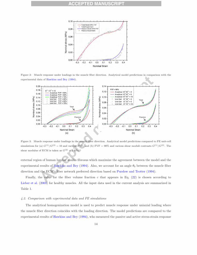
Figure 2: Muscle response under loadings in the muscle fiber direction. Analytical model predictions in comparison with the
experimental data of Hawkins and Bey (1994).
Total
Passive
(a) (b)
Total
Passive
Figure 3: Muscle response under loadings in the muscle fiber direction. Analytical model predictions compared to FE unit-cell
simulations for (a) G(1)/G(2) = 10 and various FVF, and (b) FVF = 90% and various shear moduli contrasts G(1)/G(2). The
shear modulus of ECM is taken as G(2) = 1 kPa.
external region of human lumbar anulus fibrosus which maximize the agreement between the model and the
experimental results of Hawkins and Bey (1994). Also, we account for an angle θ0 between the muscle fiber
direction and the ECM’s fiber network preferred direction based on Purslow and Trotter (1994).
Finally, the value for the fiber volume fraction c that appears in Eq. (22) is chosen according to
Lieber et al. (2003) for healthy muscles. All the input data used in the current analysis are summarized in
Table 1.
4.2. Comparison with experimental data and FE simulations
The analytical homogenization model is used to predict muscle response under uniaxial loading where
the muscle fiber direction coincides with the loading direction. The model predictions are compared to the
experimental results of Hawkins and Bey (1994), who measured the passive and active stress-strain response
14

of a healthy rat tibialis anterior muscle. The experimental data were obtained under isometric conditions,
thus the strain rate dependence on the muscle fiber stress is omitted (fr(εm0 ) = 1). All the rest input data
used in the model are shown in Table 1 and described in Section 4.1. Fig. 2 shows a very good agreement
between the model predictions and the experiments for both total (active and passive) and passive muscle
response.
The influence of fiber volume fraction and shear moduli contrast on the effective muscle response in the
muscle fiber direction is shown in Fig. 3. Comparison between the analytical model predictions and the FE
unit-cell calculations shows excellent agreement (Fig. 3). Fig. 3a shows that increased volume fractions of
ECM in a muscle may result in a manifold increase in muscle stress output when muscle is stretched in the
fiber direction. A cross-over of the total response occurs at large enough tensile strains; while at smaller
strains, the higher FVF leads to higher stresses, this response is reversed at larger strains (∼> 0.3). This
cross-over is directly attributed to the increasing role of the ECM part, which becomes rather important
at larger strains and tends to lead to higher stresses for lower FVF. On the other hand, the shear moduli
contrast between muscle fibers and ECM (and thus the isotropic behavior of the constituents) seems to have
only a weak effect on the total anisotropic tissue response, as shown in Fig. 3b.
In addition to loadings in the fiber direction, the analytical model is also able to capture the muscle
response under shear loadings across the fibers (perpendicular shear) (Fig. 4), as shown in Fig. 5. In
particular, we examine the material responses under the shear deformations Fxz and Fyz, where z-axis is
aligned in the undeformed fiber direction, for various fiber volume fractions and shear moduli contrasts
between the constituents. It is noted that analytical and FE unit-cell calculations result in the same muscle
response under either Fxz or Fyz loading. The comparisons between the analytical and numerical model
predictions presented in Fig. 5 show a very good agreement especially in the case where the activity of
the muscle fibers is taken into account. Fig. 5 also indicates that the estimates of the analytical model
under shear loadings become less accurate as the FVF is decreased and at the same time the shear moduli
contrast is increased. The analysis results show that muscle fibers control the overall muscle response when
shear strains are maintained under a certain threshold (� 0.7− 0.8 in the present case) whereas above this
threshold the effective response becomes dominated by ECM’s behavior.
Note that perpendicular shear is the only mode of simple shear in which the fibers are stretched, thus
causing a stress to develop in the direction normal to the applied shear deformation. Fig. 6 shows that, for
various FVF, a positive normal stress in the undeformed muscle fiber direction is developed when the fibers
are either active or passive. In addition, this normal stress appears to be in the same order of magnitude
with the corresponding shear stress.
15

(a)
(b)
z
xy
undeformed deformed
Figure 4: Schematic representation of perpendicular (out-of-plane) simple shear loading Fxz: (a) 2D sketch of undeformed
and deformed configurations (the dark lines represent the fibers) and (b) superimposed undeformed and deformed shape of the
unit-cell with 70% FVF and G(1)/G(2) = 2. Fibers and ECM are shown in red and blue colour respectively.
16

(a) (b)
(c) (d)
Figure 5: Perpendicular simple shear total (active and passive) and passive behavior under either Fxz or Fyz loading for
various shear moduli contrasts when (a and c) FVF = 90%, and (b and d) FVF = 70%.
(a) (b)
Figure 6: Normal stress-shear strain behavior under perpendicular simple shear loading Fxz or Fyz for various FVF when (a)
muscle fibers are fully active, and (b) muscle fibers remain passive. In both cases G(1)/G(2) = 10.
17

(a) (b)
Figure 7: Anisotropic muscle stress-strain response dependence on (a) muscle fiber’s elastic modulus, and (b) ECM’s stiffness
in its preferred direction. The values Ep = 160 kPa (stiff) and Ep = 6 kPa (compliant) were chosen for muscle fiber’s
elastic modulus as the highest and lowest values among various muscles reported in Gillies and Lieber (2011). Based on the
experimental data of Holzapfel et al. (2005) a tenfold decrease of the parameter A1 in Eq. (16), i.e. A1 = 5.3 kPa was assumed
realistic to represent a more compliant behavior in ECM’s preferred direction.
4.3. Influence of material parameters on muscle response
In the previous section the analytical model for skeletal muscle has been validated through experimental
and FE results. In this section we will focus on the analytical model estimates only and explore the effect
of a number of parameters including muscle fiber’s passive elastic modulus, ECM’s stiffness in its preferred
direction, declination angle between the muscle fibers direction and the ECM’s preferred direction, and the
velocity of contraction. The goal is to reveal the influence of micromechanical parameters on the macroscopic
muscle behavior. The parameter values presented in Table 1 are used in the analysis and the strain rate
dependence on active muscle fiber stress (εm0 = 0) is only considered when the influence of velocity of
contraction is examined.
Fig. 7 shows the effects of muscle fiber’s passive elastic modulus and ECM’s stiffness in its preferred
direction on muscle anisotropic behavior. Muscle response seems to be weakly dependent on the muscle’s
fiber modulus (Fig. 7a). On the other hand, in Fig. 7b we observe a strong dependence of the effective
response on ECM’s stiffness. An even stronger dependence of the effective response upon the angle θ0
between the muscle fibers direction and the ECM’s preferred direction can be observed in Fig. 8a. Fig. 8a
shows that even a small change in θ0 may lead to orders of magnitude different muscle stress output when
muscle is stretched in the fiber direction. Finally, in Fig. 8b we examine the influence of velocity of contraction
on muscle’s response. To do this we calculate again muscle stress from Eq. (9) by assuming that muscle
shortens or extends with a constant strain rate (εm0 = 0) based on the function fr(εm0 ) (Eq. (12)). The
isometric case (εm0 = 0) is also included in the same figure for illustration. The values used in the current
analysis for the parameters εm,min0 , kc, ke, d that enter the function fr are presented in Table 1.
18

(a) (b)
00
m
� ��
1
01.5
m
s��
� ��
1
05
m
s��
� ��
1
01.5
m
s��
��
1
05
m
s��
��
Figure 8: Anisotropic muscle stress-strain response dependence on (a) the angle θ0 between the muscle fibers direction and
the ECM’s preferred direction, and (b) velocity of active contraction.
5. Discussion
An analytical constitutive model incorporating microstructural characteristics has been developed for
skeletal muscles subjected to three-dimensional loading conditions. In order to achieve this goal a straight-
forward homogenization scheme has been used to bridge the different length scales of the muscle structure.
Due to its simplicity and numerical efficiency, the proposed muscle model has been numerically implemented
in a user-material subroutine which, in turn, allows for the simulation of three dimensional geometries of
any complexity, which is critical for biological systems.
The muscle model presented in this study has been validated by comparison with experimental data and
full field FE calculations of periodic unit-cells. The model has been found to be in very good agreement with
the experimental results and the FE results for a range of fiber volume fractions and loading conditions. The
analysis revealed that increased fractions of ECM in a muscle volume may lead to a significant stiffer muscle
response. This finding is in accord with Smith et al. (2011) who showed that ECM’s passive behavior has
significant implications in the increased muscle stiffness of spastic muscles in patients with cerebral palsy.
Since FVF depends on whether the muscle is healthy or diseased (i.e. decreasing FVF with diseased muscles
(Lieber et al., 2003)), it is important that the analytical model can predict muscle behavior accurately within
a vast range of fiber volume fractions and different material properties of the constituents.
In line with the experimental study of Meyer and Lieber (2011) the model has been able to predict that
ECM’s stiff and highly nonlinear behavior is mainly responsible for the total muscle response under stretching
in the fiber direction. Also, the model has been able to shed light on how muscle’s macroscopic response
is affected by changes of the muscle fibers’ elastic modulus, ECM’s stiffness in its preferred direction, and
declination angle between the muscle fibers direction and the ECM’s preferred direction. An important
finding of this work is that the muscle response when muscle fibers become stretched is significantly more
19

influenced by ECM’s material properties (stiffness and preferred orientation with respect to muscle fibers)
than the muscle’s fibers modulus, even if ECM accounts for only 5% of the muscle volume. A characteristic
cross-over is taking place between curves of different volume fractions at large strains where the ECM
response becomes important. In this large strain range, the homogenized response of the fiber-ECM system
gives higher stresses with decreasing FVF, while this effect is reversed at lower strains where the FVF
controls the response. Furthermore, it has been shown that significant differences in muscle response arise
between isometric and non-isometric contractions as a result of the strain rate dependence on the active
muscle fiber stress.
Most materials exhibit the so-called positive Poynting effect in the sense that under simple shear loading
conditions the material tends to expand in the direction normal to the applied shear deformation. However,
in fiber-reinforced soft tissues under perpendicular shear loading, recent experimental (Janmey et al., 2007)
and theoretical (Destrade et al., 2014) findings suggest the presence of a significant negative or reverse
Poynting effect which causes the sheared faces of the material to tend to come together; in that case a
tensile normal stress in the direction perpendicular to the shear stress is developed as a consequence of the
simple shear deformation mode. In this study, the model has been able to predict the significant reverse
Poynting effect under perpendicular simple shear loading which is accompanied with the development of
positive (tensile) normal stress in the undeformed fiber direction. As in previous studies, the normal and
shear stresses have been found to be of the same order of magnitude.
In view of the presented analytical model, we remark that equation (27) in Section 2.2 can be easily
modified to compute muscle force instead of muscle stress in the fiber direction. The 1-D equation for
muscle force, which then includes explicitly the volume fraction of fibers in the ECM, can be incorporated
into rigid-body musculoskeletal modeling frameworks through modified Hill-type muscle models in order to
be able to study how the volume fractions and material properties of muscle constituents would affect the
whole body movement.
ECM’s behavior was simplified to be transversely isotropic assuming a single preferred direction in the
material. For a more realistic material description this model can be substituted by any other model that
takes into account the internal microstructure of ECM, i.e., the presence of a fiber network at a much
smaller length scale than that of the muscle fiber itself (e.g. Chen et al., 2011; deBotton and Oren, 2013;
Tkachuk and Linder, 2012). Also, due to lack of direct measurements on muscle’s connective tissue behavior
(especially those for endomysium and perimysium which mostly interact with muscle fibers), experimental
data for another collagenous tissue (human lumbar anulus fibrosus) were used to describe ECM’s behavior
in this study. Nonetheless, the data adopted here reflect the high nonlinear and much stiffer than the muscle
fibers passive behavior of muscle’s ECM as indirectly determined by Meyer and Lieber (2011).
In the present work, a Voigt homogenization scheme has been employed to bridge the different scales of the
muscle tissue. This scheme is known to account for the microstructure only through the volume fraction of
20

the phases. For loading conditions involving no fiber stretching, i.e., longitudinal and in-plane shear loadings,
the proposed Voigt-type model is expected to deliver predictions that are stiff and become progressively more
inaccurate with increasing heterogeneity contrast. In order to overcome this shortcoming, the development of
more sophisticated homogenization schemes accounting for microstructural information beyond the volume
fractions of the phases is required. Recent progress in modeling fiber-reinforced elastomers (e.g. Agoras et al.,
2009; deBotton et al., 2006; Lopez Jımenez, 2014; Lopez-Pamies and Idiart, 2010) may prove useful to this
end. This possibility will be investigated in future work.
It should be remarked that both the numerical and the analytical models proposed in this work involve
the assumption that the muscle-fiber and ECM phases are initially perfectly bonded and remain perfectly
bonded throughout any given loading. This hypothesis is expected to be reasonably accurate, in general (i.e.,
for situations in which the muscle tissue is healthy and subjected to normal loading conditions). However,
in situations where the applied loads lead to excessively large tissue stresses or strains (e.g. during active
lengthening contraction) or when muscle tissue suffers from a disease (e.g. Duchenne muscular dystrophy),
local interfacial debonding may occur due to local damage of the transmembrane connections of the phases
(Gao et al., 2008; Virgilio et al., 2015). In general, the imperfect phase bonding is expected to lead to a
softer macroscopic response for the skeletal muscle. It would certainly be of interest to investigate the effect
of imperfect phase bonding. Specifically, in the context of a numerical homogenization scheme, the FE unit-
cells presented in Section 3 can be altered to include phase boundary imperfections by either accounting for
a third thin solid interphase at the fiber-ECM boundaries or by connecting the coincident boundary mesh
nodes of fiber and ECM with springs of different stiffnesses (Spring and Paulino, 2015; Virgilio et al., 2015;
Wurkner et al., 2013). These aspects will be examined in a future work. It should be emphasized, however,
that accounting for imperfect bonding in the context of an analytical homogenization model is a non-trivial
task (see, e.g., related work by Bigoni et al., 1998; Hashin, 1990, 1992, for linear elastic composites).
Finally, it should be pointed out that several important muscle features, such as different fiber types (fast-
or slow-twitch), grouping of fibers in motor units, fiber recruitment, muscle fatigue, and muscle residual force
enhancement are not included in the present model. The addition of such features in the model is beyond
the scope of this study and will be taken into account in a future work.
6. Conclusions
A new constitutive model for skeletal muscle tissue taking into account the volume fractions and the
material properties of its constituents is developed. Despite the limitations of the present model, to the best
knowledge of the authors, this is the first microstructural continuum model in the literature which is able
to describe the macroscopic active and passive behavior of skeletal muscles. The model is used to shed light
on how several micromechanical changes may affect muscle’s macroscopic behavior. Our analysis, in accord
21

with former literature, suggests that changes in intramuscular connective tissue may have a significant role
in the increased muscle stiffness resulted by diseases, such as spasticity. Such observations may lead to new
therapeutic treatments on skeletal muscle disease-related dysfunctions. In addition, the constitutive model is
numerically implemented in a finite-element framework which provides the opportunity to investigate clinical
related problems in a multiscale framework by analyzing three-dimensional anatomical muscle structures.
Acknowledgments
K.D. would like to acknowledge partial support from the European Research Council (ERC) under the
European Unions Horizon 2020 research and innovation program (Grant Agreement No. 636903).
Appendix
In this appendix we describe the numerical implementation of the analytical constitutive model in the
context of the finite element method. In view of the non-linearity and the rate dependence of the model,
the finite element solution is developed incrementally. The constitutive calculations are carried out at the
element Gauss integration points. In particular, at a given Gauss point, the directional vector in the reference
configuration m0, the homogenized solution (F n, σn, εm0 |n) at time tn as well as the average deformation
gradient F n+1 at time tn+1 = tn +Δt are known, and the problem is to determine (σn+1, εm0 |n+1, mn+1).
The constitutive calculations at the Gauss points are carried out in the following order:
F n+1 =(det F n+1
)−1/3
F n+1, (31)
Bn+1 = F n+1 · FT
n+1, (32)
mn+1 =1
|F n+1 ·m0|F n+1 ·m0, (33)
λm|n+1 =
√m0 · F
T
n+1 · F n+1 ·m0, (34)
εm0 |n+1 = λm|n+1 − 1, (35)
˙εm
0 |n+1 =εm0 |n+1 − εm0 |n
Δt, (36)
G = c ·G(1) + (1− c) ·G(2), (37)
K = c ·K(1) + (1 − c) ·K(2), (38)
σ(1)0 |n+1 = σmaxfa|n+1fe(ε
m0 |n+1)fr( ˙ε
m
0 |n+1) + fp(1)(εm0 |n+1), (39)
22

σ(2)0 |n+1 = f (2)
p (λm|n+1, θ0), (40)
σ0|n+1 = c · σ(1)0 |n+1 + (1− c) · σ(2)
0 |n+1, (41)
σn+1 = (1 + εm0 |n+1) σ0|n+1, (42)
σi|n+1 =G
det F n+1
(Bn+1 − 1
3tr(Bn+1
)δ
)+ K
(det F n+1 − 1
)δ, (43)
σa|n+1 = σn+1 mn+1 mn+1, (44)
σ|n+1 = σi|n+1 + σa|n+1. (45)
The “implicit” version of ABAQUS is used, in which the finite element formulation is based on the weak
form of the equilibrium equations, the solution is carried out incrementally, and the discretized nonlinear
equations are solved by using Newton’s method. The Jacobian of the equilibrium Newton-loop requires the
so-called “linearization moduli” of the algorithm that handles the constitutive equations; these moduli are
defined in terms of a fourth-order tensor C that relates the variation of stress ∂σ to the variation of strain
∂ε over the increment under consideration:
∂σ = C : ∂ε =(Ci
+ Ca): ∂ε. (46)
The details of the derivation of Ciand Ca
are reported in Suchocki (2011) and Spyrou (2009) respectively.
Here we note that
Ci
ijkl =G
J
[1
2
(δikBjl + Bikδjl + δilBjk + Bilδjk
)−2
3δijBkl − 2
3Bijδkl +
2
9δijδklBmm
]+ K
(2J − 1
)δijδkl,
(47)
and
Ca
ijkl = (1 + εm0 )(σ0 +D)Hijkl + σ Aijkl , (48)
with
D = (1 + εm0 )
(∂σ0
∂εm0+
1
Δt
∂σ0
∂ ˙εm
0
), (49)
Hijkl = mimjmkml, (50)
Aijkl =1
2(δik mj + δjk mi) ml +
1
2(δil mj + δjl mi) mk − 2Hijkl. (51)
In equations 47–51 all quantities are evaluated at the end of the increment under consideration, i.e., at
t = tn+1. It is noted that the fourth-order tensor C has both the “minor” and “major” symmetries, i.e.,
Cijkl = Cjikl = Cijlk = Cklij . (52)
23

References
ABAQUS, 2009. Dassault Systems Abaqus. ABAQUS/Standard Version 6.9, Simulia Corp.
Agoras, M., Lopez-Pamies, O., Castaneda, P.P., 2009. A general hyperelastic model for incompressible fiber-reinforced elas-
tomers. J. Mech. Phys. Solids 57, 268–286.
Bigoni, Z., Serkov, S.K., Valentini, M., Movchan, A.B., 1998. Asymptotic models of dilute composites with imperfectly bonded
inclusions. Int. J. Solids and Structures 35, 3239–3258.
Bleiler, C., Castaneda, P.P., Rohrle, O., 2015. Towards effective mechanical properties of skeletal muscle tissue via homogeni-
sation. Proc. Appl. Math. Mech. 15, 83–84.
Blemker, S.S., Pinsky, P.M., Delp, S.L., 2005. A 3D model of muscle reveals the causes of nonuniform strains in the biceps
brachii. J. Biomech. 38, 657–665.
Bol, M., Reese, S., 2008. Micromechanical modelling of skeletal muscles based on the finite element method. Comput. Methods
Biomech. Biomed. Engin. 11, 489–504.
Bol, M., Weikert, R., Weichert, C., 2011. A coupled electromechanical model for the excitation-dependent contraction of
skeletal muscle. J. Mech. Behav. Biomed. Mater. 4, 1299–1310.
Ceelen, K.K., Oomens, C.W.J., Baaijens, F.P.T., 2008. Microstructural analysis of deformation-induced hypoxic damage in
skeletal muscle. Biomech. Model. Mechanobiol. 7, 277–284.
Chen, H., Liu, Y., Zhao, X., Lanir, Y., Kassab, G.S., 2011. A micromechanics finite-strain constitutive model of fibrous tissue.
J. Mech. Phys. Solids 59, 1823–1837.
deBotton, G., Hariton, I., Socolsky, E.A., 2006. Neo-Hookean fiber-reinforced composites in finite elasticity. J. Mech. Phys.
Solids 54, 533–559.
deBotton, G., Oren, T., 2013 Analytical and numerical analyses of the micromechanics of soft fibrous connective tissues.
Biomech. Model. Mechanobiol. 12, 151–166.
Destrade, M., Horgan, C.O., Murphy, J.G., 2014. Dominant negative Poynting effect in simple shearing of soft tissues. J. Eng.
Math. 95, 87–98.
Ehret, A.E., Bol, M., Itskov, M., 2011. A continuum constitutive model for the active behaviour of skeletal muscle. J. Mech.
Phys. Solids 59, 625–636.
Emery, A.E.H., 2002. The muscular dystrophies. Lancet 359, 687–695.
Gao, Y., Wineman, A.S., Waas, A.M., 2008. Mechanics of muscle injury induced by lengthening contraction. Ann. Biomed.
Eng. 36, 1615–1623.
Gindre, J., Takaza, M., Moerman, K.M., Simms, C.K., 2013. A structural model of passive skeletal muscle shows two rein-
forcement processes in resisting deformation. J. Mech. Behav. Biomed. Mater. 22, 84–94.
Gillies, A.R., Lieber, R.L., 2011. Structure and function of the skeletal muscle extracellular matrix. Muscle Nerve 44, 318–331.
Hashin, Z., 1990. Thermoelastic properties of fiber composites with imperfect interface. Mechanics of Materials 8, 333–348.
Hashin, Z., 1992. Extremum principles for elastic heterogeneous media with imperfect interfaces and their application to
bounding of effective moduli. J. Mechanics and Physics of Solids 40, 767–781.
Hawkins, D., Bey, M., 1994. A comprehensive approach for studying muscle-tendon mechanics. J. Biomech. Eng. 116, 51–55.
Heidlauf, T., Rohrle, O., 2014. A multiscale chemo-electro-mechanical skeletal muscle model to analyze muscle contraction and
force generation for different muscle fiber arrangements. Front. Physiol. 5, 498/1–14.
Hernandez-Gascon, B., Grasa, J., Calvo, B., Rodrıguez, J.F., 2013. A 3D electro-mechanical continuum model for simulating
skeletal muscle contraction. J. Theor. Biol. 335, 108–118.
Holzapfel, G.A., Gasser, T.C., Ogden, R.W., 2000. A new constitutive framework for arterial wall mechanics and a comparative
study of material models. J. Elasticity 61, 1–48.
24

Holzapfel, G.A., Schulze-Bauer, C.A.J., Feigl, G., Regitnig, P., 2005. Single lamellar mechanics of the human lumbar anulus
fibrosus. Biomech. Model. Mechanobiol. 3, 125–140.
Holzapfel, G.A., Ogden, R.W., 2015. On the tension-compression switch in soft fibrous solids. Eur. J. Mech. A-Solid 49,
561–569.
Huijing, P.A., 1999. Muscle as a collagen fiber reinforced composite: a review of force transmission in muscle and whole limb.
J. Biomech. 32, 329–345.
Janmey, P.A., McCormick, M.E., Rammensee, S., Leight, J.L., Georges, P.C., MacKintosh, F.C., 2007 Negative normal stress
in semiflexible biopolymer gels. Nat. Mater. 6, 48–51.
Javili, A., Chatzigeorgiou, G., Steinmann, P., 2013. Computational homogenization in magneto-mechanics. Int. J. Solids.
Struct. 50, 4197–4216.
Johansson, T., Meier, P., Blickhan, R., 2000. A finite-element model for the mechanical analysis of skeletal muscles. J. Theor.
Biol. 206, 131–149.
Jozsa, L., Thoring, J., Jarvinen, M., Kannus, P., Lehto, M., Kvist, M., 1988. Quantitative alterations in intramuscular
connective tissue following immobilization: an experimental study in the rat calf muscles. Exp. Mol. Pathol. 49, 267–278.
Kjær, M., 2004. Role of extracellular matrix in adaptation of tendon and skeletal muscle to mechanical loading. Physiol. Rev.
84, 649–698.
Lemos, R.R., Epstein, M., Herzog, W., Wyvill, B., 2004. A framework for structured modeling of skeletal muscle. Comput.
Methods Biomech. Biomed. Engin. 7, 305–317.
Liang, Y., McMeeking, R.M., Evans, A.G., 2006. A finite element simulation scheme for biological muscular hydrostats. J.
Theor. Biol. 242, 142–150.
Lieber, R.L., Runesson, E., Einarsson, F., Friden, J., 2003. Inferior mechanical properties of spastic muscle bundles due to
hypertrophic but compromised extracellular matrix material. Muscle Nerve 28, 464–471.
Lopez Jımenez, F., 2014. Modeling of soft composites under three-dimensional loading. Compos. Part B Eng. 59, 173–180.
Lopez-Pamies, O., Idiart, M.I., 2010. Fiber-reinforced hyperelastic solids: a realizable homogenization constitutive theory. J.
Eng. Math. 68, 57–83.
Lopez-Pamies, O., Goudarzi, T., Danas, K., 2013. The nonlinear elastic response of suspensions of rigid inclusions in rubber.
II. A simple explicit approximation for finite-concentration suspensions. J. Mech. Phys. Solids 61, 19–37.
Mann, C.J., Perdiguero, E., Kharraz, Y., Aguilar, S., Pessina, P., Serrano, A.L., Munoz-Canoves, P., 2011 Aberrant repair and
fibrosis development in skeletal muscle. Skelet. Muscle 1, 1–20.
Martins, J.A.C., Pires, E.B., Salvado, R., Dinis, P.B., 1998. A numerical model of passive and active behavior of skeletal
muscles. Comput. Methods Appl. Mech. Eng. 151, 419–433.
Mbiakop, A., Constantinescu, A., Danas, K., 2015. An analytical model for porous single crystals with ellipsoidal voids. J.
Mech. Phys. Solids 84, 436–467.
Meyer, G.A., Lieber, R.L., 2011. Elucidation of extracellular matrix mechanics from muscle fibers and fiber bundles. J.
Biomech. 44, 771–773.
Michel, J.C., Moulinec, H., Suquet, P., 1999. Effective properties of composite material with periodic microstructure: a
computational approach. Comput. Methods Appl. Mech. Eng. 172, 109–143.
Purslow, P.P., 1989 Strain-induced reorientation of an intramuscular connective tissue network: implications for passive muscle
elasticity. J. Biomech. 22, 21–31.
Purslow, P.P., Trotter, J.A., 1994. The morphology and mechanical properties endomysium in series-fibred muscles: variations
with muscle length. J. Muscle Res. Cell. Motil. 15, 299–308.
Rohrle, O., Pullan, A.J., 2007. Three-dimensional finite element modelling of muscle forces during mastication. J. Biomech.
40, 3363–3372.
25

Sharafi, B., Blemker, S.S., 2010. A micromechanical model of skeletal muscle to explore the effects of fiber and fascicle geometry.
J. Biomech. 43, 3207–3213.
Sharafi, B., Blemker, S.S., 2011. A mathematical model of force transmission from intrafascicularly terminating muscle fibers.
J. Biomech. 44, 2031–2039.
Smith, L.R., Lee, K.S., Ward, S.R., Chambers, H.G., Lieber, R.L., 2011. Hamstring contractures in children with spastic
cerebral palsy result from a stiffer extracellular matrix and increased in vivo sarcomere length. J. Physiol. 589, 2625–2639.
Spring, D.W., Paulino, G.H., 2015. Computational homogenization of the debonding of particle reinforced composites: The
role of interphases in interfaces. Comp. Mater. Sci. 109, 209–224.
Spyrou, L.A., 2009. Muscle and tendon tissues: constitutive modeling, numerical implementation and applications. Dissertation,
University of Thessaly.
Spyrou, L.A., Aravas, N., 2011. Muscle and tendon tissues: constitutive modeling and computational issues. J. Appl. Mech.
78, 041015/1–10.
Spyrou, L.A., Aravas, N., 2012. Muscle-driven finite element simulation of human foot movements. Comput. Methods Biomech.
Biomed. Engin. 15, 925–934.
Suchocki, C., 2011. A finite element implementation of Knowles stored-energy function: theory, coding and applications. Arch.
Mech. Eng. 58, 319–346.
Thacker, B.E., Tomiya, A., Hulst, J.B., Suzuki, K.P., Bremner, S.N., Gastwirt, R.F., Greaser, M.L., Lieber, R.L., Ward, S.R.,
2012. Passive mechanical properties and related proteins change with botulinum neurotoxin A injection of normal skeletal
muscle. J. Orthop. Res. 30, 497–502.
Tkachuk, M., Linder, C., 2012. The maximal advance path constraint for the homogenization of materials with random network
microstructure. Philos. Mag. 92, 2779–2808.
Trotter, J.A., Richmond, F.J.R., Purslow, P.P., 1995. Functional morphology and motor control of series-fibered muscles.
Exerc. Sport Sci. Rev. 23, 167–214.
Van Leeuwen, J.L., Kier, W.M., 1997. Functional design of tentacles in squid: linking sarcomere ultrastructure to gross
morphological dynamics. Philos. Trans. R. Soc. Lond. B Biol. Sci. 352, 551–571.
Van Loocke, M., Lyons, C.G., Simms, C.K., 2006. A validated model of passive muscle in compression. J. Biomech. 39,
2999–3009.
Virgilio, K.M., Martin, K.S., Peirce, S.M., Blemker, S.S., 2015. Multiscale models of skeletal muscle reveal the complex effects
of muscular dystrophy on tissue mechanics and damage susceptibility. Interface Focus 5, 20140080/1–10.
Wurkner, M., Berger, H., Gabbert, U., 2013. Numerical study of effective elastic properties of fiber reinforced composites with
rhombic cell arrangements and imperfect interface. Int. J. Eng. Sci. 63, 1–9.
Zajac, F.E., 1989. Muscle and tendon: properties, models, scaling and application to biomechanics and motor control. Crit.
Rev. Biomed. Eng. 17, 359–411.
26
View publication statsView publication stats