a human-robot collaborative learning system using a...
TRANSCRIPT

1
Ben-Gurion University of the Negev
Faculty of Engineering Sciences
Department of Industrial Engineering and Management
Research Proposal:
A Human-Robot Collaborative
Learning System Using a Virtual
Reality Telerobotic Interface
רובוטי במציאות -משולבת ממשק טלהרובוט לומדת -מערכת אדם
מדומה
Submitted in partial fulfillment of the requirements for the degree of
Doctor of Philosophy in Engineering
Uri Kartoun
October, 2003
2
Ben-Gurion University of the Negev
Faculty of Engineering Sciences
Department of Industrial Engineering and Management
Research Proposal:
A Human-Robot Collaborative Learning System Using a
Virtual Reality Telerobotic Interface
רובוטי במציאות מדומה-רובוט לומדת משולבת ממשק טלה-מערכת אדם
Submitted in partial fulfillment of the requirements for the degree of
Doctor of Philosophy in Engineering
Uri Kartoun
Advisors: Prof. Helman Stern
Prof. Yael Edan
Author’s signature:______________________ Date:__________
Advisor’s signature:_____________________ Date:__________
Advisor’s signature:_____________________ Date:__________
Departmental committee chairman’s signature:____________ Date:__________
3
A Human-Robot Collaborative Learning System Using a Virtual
Reality Telerobotic Interface
Abstract
This research focuses on the development of a telerobotic system that employs several state-
action policies to carry out a task using on-line learning with human operator (HO) intervention
through a virtual reality (VR) interface. The case-study task is to empty the contents of an unknown
bag for subsequent scrutiny.
A system state is defined as a condition that exists in the system for a significant period of
time and consists of the following sub-states: 1) the bag which includes a feature set such as its type
(e.g., plastic bag, briefcase, backpack, or suitcase) and its condition (e.g., open, close, orientation,
distortions in bag contour, partial hiding of a bag, changing of handle lengths); 2) the robot (e.g.,
gripper spatial coordinates, home position, idle, performing a task); 3) other objects (e.g., contents
that fell out of the bag, obstructions) and 4) environmental conditions such as illumination (e.g., day
or night).
A system action takes the system to a new state. Action examples include initial grasping
point, lift and shake trajectory, re-arranging the position of a bag to prepare it for better grasping and
enable the system to verify if all the bag contents have been extracted.
Given the system state and a set of actions, a policy is a set of state-action pairs to perform a
robotic task. The system starts with knowledge of the individual operators of the robot arm, such as
opening and closing the gripper, but it has no policy for deciding when these operators are
appropriate, nor does it have knowledge about the special properties of the bags. A policy is defined
as the best action for a given state. The system learns this policy from experience and human
guidance. A policy is found to be beneficial if a bag was grabbed successfully and all its contents
have been extracted.
Learning the optimal policy for classifying system states will be conducted using two soft
computing methods: 1) on-line adaptive resonance theory (ART) and 2) off-line support vector
machines (SVMs). The inference of these methods will be a recommendation for a set of possible
grasping points. Their recognition accuracy will be compared for a set of test cases. Reinforcement
learning (e.g., Q-learning) will be used to find the best action (e.g., determining the optimal grasping
point followed by a lift and shake trajectory) for a given state.
When unknown system states are identified, the HO suggests solutions (policies) through a
VR interface and the robot decides to accept or reject them. The HO monitors the interactions of the
telerobot on-line and controls the system through the VR interface. Policy examples are to let the
HO classify the type of a bag (e.g., a briefcase) when it was recognized mistakenly as a different
type (e.g., a suitcase) and to provide a set of possible grasping points by the HO when the system
finds it difficult to recognize points that are beneficial for completing the task. When HO
intervention is found to be beneficial, the system learns, and its dependence on the HO decreases.
For testing the above, an advanced virtual reality (VR) telerobotic bag shaking system is
proposed. It is assumed that several kinds of bags are placed on a platform. All locks have been
removed and latches and zippers opened. The task of the system is to empty the contents of an
unknown bag onto the platform for subsequent scrutiny. It is assumed that the bag has already
passed X-ray inspection to ensure the bag is not empty and does not contain obvious explosives
(e.g., mines, gun bullets).

4
HO collaboration is conducted via a VR interface, which has an important role in the system.
The HO either manipulates the 3D robot off-line, suggests solutions (e.g., the robot learns an optimal
grasping location and avoids others) or changes and adds lifting and shaking policies on-line. When
the robot encounters a situation it cannot handle, it relies on HO intervention. HO intervention will
be exploited by the system to support the evolution of autonomy in two ways: first, by providing
input to machine learning to support system adaptation, and second, by characterizing those
situations when operator intervention is necessary when autonomous capabilities fail. Finally,
measuring the amount of required operator intervention provides a metric for judging the system's
level of autonomy - the less intervention, the higher the level of autonomy.
Keywords: support vector machines, ART neural networks, robot learning, machine vision,
virtual reality, human-robot collaboration, telerobotics

5
רובוטי במציאות מדומה-רובוט לומדת משולבת ממשק טלה-מערכת אדם
תקציר
פעולה לביצוע משימה תוך -רובוטית המשתמשת במספר אסטרטגיות מצב-מחקר זה מתמקד בפיתוח מערכת טלה
שימוש בלימוד בשילוב התערבות אדם דרך ממשק מציאות מדומה. המשימה שהוגדרה לבחינת המערכת הינה ריקון תכנו
של תיק בלתי מזוהה לשם ביצוע בדיקה ומעקב.
התיק( 1מצב מערכת מוגדר כתנאי הקיים במערכת לאורך מחזור זמן משמעותי ומורכב מתתי המצבים הבאים:
, פתוח, לדוגמא) ומצבו, שקית פלסטיק, תיק מסמכים, מזוודה, או תרמיל גב( לדוגמא) סוגוהכולל סדרת מאפיינים כגון
, קואורדינטות לדוגמא) הרובוט( 2 ;יוותי קווי מתאר, הסתרה חלקית של הידית, שינויים באורך הידית(סגור, כיוונו, ע
, תוכן שנפל מהתיק, מכשולים( ו לדוגמא) אובייקטים אחרים( 3 ;מרחביות של התפסנית, עמדת בית, בטלה, מבצע משימה(
, יום או לילה(.לדוגמאכגון תאורה ) תנאים סביבתיים( 4 -
מערכת מובילה את המערכת למצב חדש. דוגמאות לפעולות כוללות נקודת אחיזה התחלתית, מסלול הרמה פעולת
ונענוע, ארגון מחדש של מיקום התיק בכדי להכינו לאחיזה טובה יותר ובדיקה האם כל תוכן התיק חולץ.
ביצוע משימה רובוטית. פעולה ל-מצב המערכת וסידרה של פעולות, אסטרטגיה הינה אוסף של זוגות מצב ןבהינת
לזרוע הרובוטית, כגון פתיחת וסגירת התפסנית, אך אין לה תהמערכת מתחילה את פעולתה עם ידע הכולל תכונות ייחודיו
כן, אין לה ידע לגבי המאפיינים המיוחדים של התיקים. אסטרטגיה מוגדרת -אסטרטגיה להחליט מתי יש להשתמש בהן, כמן
ומהנחייה על ידי אדם. ןר בעבור מצב נתון. המערכת לומדת את האסטרטגיה הזו מניסיוכביצוע הפעולה הטובה ביות
אסטרטגיה תמצא יעילה אם התיק נאחז בהצלחה ותוכנו רוקן.
לימוד האסטרטגיה המיטבית למטרת ביצוע סיווג מצבי המערכת יתבצע תוך שימוש בשתי שיטות חישוב נבונות:
1 )On-line Artificial Resonance Theory (ART) 2 -ו )Off-line Support Vector Machines (SVMs) .
ההסקה של כל אחת מהשיטות תהווה המלצה לאוסף של נקודות אחיזה אפשרויות. דיוק הזיהוי של שתי השיטות יושווה
א את ( יבוצע בכדי למצוQ-learning, לדוגמא) Reinforcement Learning (RL) -עבור מגוון מקרים. שימוש ב
, קביעת נקודת האחיזה הטובה ביותר ובעקבותיה מסלול הרמה ונענוע( בעבור מצב נתון.לדוגמאהפעולה הטובה ביותר )
כאשר מזוהים מצבי מערכת בלתי מוכרים, האדם מציע פתרונות )אסטרטגיה( דרך ממשק מציאות מדומה והרובוט
רובוטית ושולט עליה דרך ממשק המציאות המדומה. -להמחליט אם לקבל או לדחות אותם. האדם משגיח על המערכת הט
, תיק מסמכים( כאשר הוא זוהה בטעות כסוג אחר לדוגמאדוגמאות לאסטרטגיות הינן לאפשר לאדם לסווג את סוג התיק )
, מזוודה( ולספק אוסף של נקודות אחיזה אפשריות כאשר המערכת מתקשה בזיהוי נקודות החיוניות להשלמת לדוגמא)
. כאשר התערבות האדם נמצאת מועילה, המערכת לומדת, ותלותה באדם פוחתת.המשימה
רובוטית הנשלטת מממשק מציאות מדומה אשר תפקידה -בכדי לבחון את אשר צוין מעלה, מוצעת מערכת טלה
ימת לרוקן תיקים. ניתן להניח שכמה סוגי תיקים מונחים על שולחן. כל מנעולי התיקים הוסרו והרוכסנים נפתחו. מש
המערכת הינה לרוקן את תוכנו של תיק שאינה מכירה על השולחן לשם ביצוע בדיקה ומעקב. הנחה נוספת הינה שהתיק
, מוקשים, כדורי רובה(.לדוגמאנפץ מוכרים ) יהנבדק כבר עבר בדיקת רנטגן בכדי להבטיח שאינו ריק ואינו מכיל חומר

6
ציאות מדומה שהינו בעל חשיבות רבה עבור המערכת. שיתוף הפעולה בין הרובוט לאדם מבוצע דרך ממשק מ
, הרובוט לומד נקודות אחיזה מיטביות, ומתעלם לדוגמא, להציע פתרונות )off-lineהאדם יכול לשלוט על הרובוט במצב
. כאשר הרובוט נתקל בסיטואציה שאינו מכיר, הוא חייב on-lineמאחרות(, או לשנות ולהוסיף אסטרטגיית הרמה ונענוע
להסתמך על התערבות האדם. התערבות האדם תנוצל על ידי המערכת בכדי לתמוך בהתפתחות המערכת בשתי דרכים:
בראשונה, על ידי אספקת קלט למכונה לומדת בכדי לתמוך בהסתגלות המערכת, ובשנית, על ידי אפיון מצבים בהם
כמות התערבות האדם מספקת מדד לשיפוט רמת התערבות האדם נחוצה כאשר יכולות אוטונומיות נכשלות. לבסוף, מדידת
ככל שקיימת פחות התערבות, כך גדלה רמת האוטונומיות. -האוטונומיות של המערכת
, support vector machines ,ART neural networks ,robot learning ,machine visionמילות מפתח:
virtual reality ,human-robot collaboration ,telerobotics

7
Table of Contents
1. INTRODUCTION ........................................................................................................... 9
2. THE RESEARCH.......................................................................................................... 12
2.1. RESEARCH OBJECTIVES ...................................................................................................... 12 2.2. RESEARCH SIGNIFICANCE .................................................................................................... 12 2.3. EXPECTED CONTRIBUTIONS AND INNOVATIONS ..................................................................... 13
3. SCIENTIFIC BACKGROUND ...................................................................................... 14
3.1. TELEROBOTICS ................................................................................................................. 14 3.2. VIRTUAL REALITY ............................................................................................................. 17 3.3. ROBOT LEARNING .............................................................................................................. 18
4. RESEARCH METHODOLOGY .................................................................................... 24
4.1. PROBLEM DEFINITION AND NOTATION .................................................................................. 24 4.2. PERFORMANCE MEASURES .................................................................................................. 26 4.3. METHODOLOGY ................................................................................................................. 26
4.3.1. System architecture .................................................................................................. 26 4.3.2 . System flow and operational stages ........................................................................... 28
4.4. PROCEDURES ................................................................................................................. 30 4.4.1 . Image processing ..................................................................................................... 31
4.4.2 . Adaptive resonance theory........................................................................................ 32
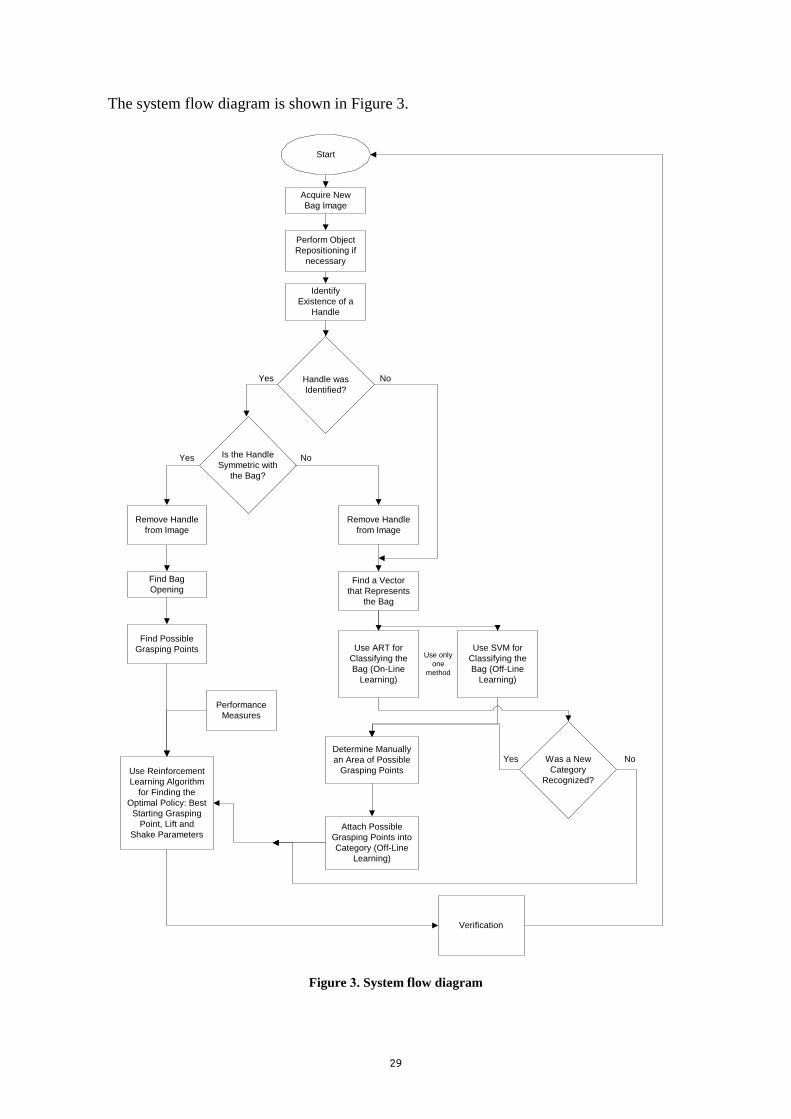
4.4.3 . Support vector machines .......................................................................................... 35
4.4.4 . Reinforcement learning ............................................................................................ 36 4.5. TESTING AND VALIDATION .................................................................................................. 37
4.5.1. Physical experimental setting ................................................................................... 37 4.5.2 . Performance evaluation ........................................................................................... 38
5. RESEARCH PLAN ....................................................................................................... 39
5.1. RESEARCH STAGES ............................................................................................................. 39 5.2. RESEARCH ROADMAP ......................................................................................................... 41
6. MS.C. THESIS - VIRTUAL REALITY TELEROBOTIC SYSTEM ................................. 42
6.1. INTRODUCTION ................................................................................................................. 42 6.1.1. Description of the problem ....................................................................................... 42 6.1.2 . Objective ................................................................................................................ 42
6.2. METHODOLOGY ................................................................................................................. 43 6.2.1 . Task definition ......................................................................................................... 43
6.2.2 . System architecture .................................................................................................. 43
6.2.3 . Tools ..................................................................................................................... 45
6.2.4 . Physical Description of the System ............................................................................ 46
6.2.5 . The virtual environment ........................................................................................... 47
6.2.6 . Operational stages ................................................................................................... 48 6.3. SYSTEM TEST AND VALIDATION ........................................................................................... 49
6.3.1. Calibration ............................................................................................................. 49 6.3.2 . System learning curve experiment ............................................................................. 51
6.3.3 . Summary ................................................................................................................. 52
7. REFERENCES .......................................................................................................... 53

8
List of Figures
FIGURE 1. DIFFERENT KINDS OF BAGS ................................................................................................ 25
FIGURE 2 . SYSTEM ARCHITECTURE .................................................................................................... 26
FIGURE 3 . SYSTEM FLOW DIAGRAM ................................................................................................... 29
FIGURE 4 . SEPARATING HANDLE FROM BAG EXAMPLE ........................................................................ 31
FIGURE 5 . ART-1 ARCHITECTURE METHODOLOGY ............................................................................. 32
FIGURE 6 . IMAGE PROCESSING OPERATIONS FOR A SAMPLE BAG IMAGE .............................................. 33
FIGURE 7 . AN EXAMPLE FOR ONE IMAGE PORTION .............................................................................. 34
FIGURE 8 . MULTI-CLASS METHODOLOGY USING ONE VS. ALL (OVA) APPROACH ................................ 35
FIGURE .9 1-STEP Q-LEARNING ALGORITHM ...................................................................................... 36
FIGURE 11. EXPERIMENTAL SETUP ..................................................................................................... 37
FIGURE 11 . CLIENT-SERVER COMMUNICATION ARCHITECTURE ........................................................... 43
FIGURE 12. VIRTUAL REALITY TELEROBOTIC SYSTEM ARCHITECTURE ................................................. 44
FIGURE 13 . VR ROBOT GRIPPER EDGE ................................................................................................ 47
FIGURE 14 . VR ROBOT HOME-POSITION ............................................................................................ 48
FIGURE 15 . CALIBRATION EXPERIMENT FLOW CHART ......................................................................... 50
FIGURE 16 . “A255” ROBOT, PLASTIC BAG, PLATFORM AND TEN ELECTRONIC COMPONENTS .................. 51
FIGURE 17 . LEARNING CURVE EXPERIMENT RESULTS .......................................................................... 52
List of Tables
TABLE 1 . SUMMARY OF TELEROBOTICS RELATED WORKS ................................................................... 15 TABLE 2 . SUMMARY OF HUMAN-ROBOT COLLABORATION RELATED WORKS ......................................... 17 TABLE 3 . SUMMARY OF VR RELATED WORKS ..................................................................................... 18 TABLE 4 . SUMMARY OF ROBOT LEARNING RELATED WORKS................................................................ 22 TABLE 5 . LEARNING TECHNIQUES ...................................................................................................... 23 TABLE 6 . SYSTEM OPERATIONAL STAGES ........................................................................................... 28 TABLE 7 . BAG SAMPLE EXAMPLE ANALYSIS ........................................................................................ 34
List of Appendices
APPENDIX I: TELEROBOTICS APPLICATIONS ........................................................................................ 62
APPENDIX II: HUMAN-ROBOT COLLABORATION .................................................................................. 63
APPENDIX III: VIRTUAL REALITY APPLICATIONS................................................................................. 64
APPENDIX IV: VIRTUAL SOFTWARE EDITING SYSTEMS ........................................................................ 67
APPENDIX V: ROBOT LEARNING ......................................................................................................... 70
APPENDIX VI: ART-1......................................................................................................................... 72
APPENDIX VII: SUPPORT VECTOR MACHINES ...................................................................................... 78
APPENDIX VIII: REINFORCEMENT LEARNING ..................................................................................... 85
APPENDIX IX: VR ROBOTIC ENVIRONMENT ........................................................................................ 88
APPENDIX X: OPERATIONAL CONTROL PANELS ................................................................................... 90
APPENDIX XI: KINEMATICS .............................................................................................................. 105
APPENDIX XII: TRANSFORMATION MATRIX ...................................................................................... 109

9
1 Introduction
Building robotic systems that learn to perform a task has been acknowledged as one of the
major challenges facing artificial intelligence [Connell and Mahadevan, 1993]. Self-improving robots
can relieve humans from much of the drudgery of programming and potentially allow their operation in
unknown and dynamic environments [Connell and Mahadevan, 1993]. Progress towards this goal can
contribute to intelligent systems by advancing the understanding of how to successfully integrate
disparate abilities such as perception, planning, learning, and action.
Robotics is one of the most challenging applications of machine learning techniques. It is
characterized by direct interaction with a real world, sensory feedback and complex control system
[Kreuziger, 1992]. Learning should lead to faster or more reliable solution executions or to the ability to
solve problems the robot was not able to solve before or to a more simple system. Possible applications
of machine learning to robotics are given: 1) World model and elementary (sensor-based) actions [e.g.,
Kerr and Compton, 2003]: learning of object properties (e.g., geometry), world exploration (e.g., finding
objects, determining obstacles), learning of elementary actions in the world (e.g., effects of actions),
learning of elementary actions with objects (e.g., manipulation of an object) and learning to recognize /
classify states in the internal world model; 2) Sensors [e.g., Harvey et al.]: learning of classifiers for
objects based on image data, learning of sensor strategies / plans (e.g., how to monitor an action to
ensure the correct execution or how to determine certain states of the real world); 3) Error analysis [e.g.,
Scheffer and Joachims, 1999]: learning of error recognition, error diagnosis and error repairing rules; 4)
Planning [e.g., Theocharous and Mahadevan, 2002]: improvement (speed-up) of planning module (e.g.,
planning macros, control rules), learning of action rules or plans (i.e., how to solve a sub (task) in
principle), learning of couplings between typical task classes and related action plans (e.g., generalized
action plan for a set of tasks), learning at the task level (e.g., which geometrical arrangements / action
plans satisfy certain functional specifications).
Bhanu et al., 2001, presents the design, implementation and testing of a real-time system using
computer vision and machine learning techniques to demonstrate learning in a miniature mobile robot.
The miniature robot learns to navigate a maze using several reinforcement learning based algorithms.
Carreras et al., 2002, propose a Neural-Q_learning approach designed for on-line learning of
simple and reactive robot behaviors. In this approach, the Q_function is generalized by a multi-layer
neural network allowing the use of continuous states and actions. The algorithm uses a database of the
most recent learning samples to accelerate and guarantee the convergence. Each Neural-Q_learning
function represents an independent, reactive and adaptive behavior which maps sensorial states to robot

11
control actions. A group of these behaviors constitutes a reactive control scheme designed to fulfill
simple missions.
The environments into which a robot system is placed may have a variety of unfamiliar objects,
materials and lighting conditions, making the perceptual and manipulation task difficult without the use
of a significant number of domain-dependent techniques. Imaging sensors are widely employed in robot
applications due to the large amount of information they supply [Unger and Bajcsy, 1996]. Vision-based
grasping and retrieval of objects is an important skill in many tasks [Unger and Bajcsy, 1996]. A robotic
system having the ability to perceive pertinent target object features, and the ability to select viable
grasp approach for a robotic arm can perform many useful functions [Unger and Bajcsy, 1996]. Possible
scenarios for such a system range from the handling of explosive materials in dangerous environments
to the assistance to people with physical disabilities in household environments.
Nowadays, robots are moving off factory production lines and into our everyday lives. Unlike
stationary and pre-engineered factory buildings, an everyday environment, such as an office, museum,
hospital, or home, is an open and dynamic place where robots and humans can co-exist and cooperate.
The office robot, Jijo-2 [Asoh et al., 2001], was built as a testbed for autonomous intelligent systems
that interact and learn in the real world. Jijo-2’s most notable properties are its communication and
learning skills: it can communicate with humans through a sophisticated Japanese spoken-dialogue
system, and it navigates by using models that it learns by itself or through human supervision. It
achieves the former through a combination of a microphone array, speech recognition module, and
dialogue management module. It achieves the latter through statistical learning procedures by which the
robot learns landmarks or features of its environment that let it construct useful models for navigation.
Within the context of robots controlled through the web [e.g., Stein, 2000], research has
traditionally focused on the global system functionality, including the way of interaction between the
user and the robot. Recent results in different robotics areas have demonstrated the potential role of
several techniques from pattern recognition and machine learning domains, although very few works
specifically addressed on-line robots, where object recognition is directly performed by the user [Sanz
and Sánchez, 2003]. Human-robot interaction (HRI) can be defined as the study of humans, robots, and
the ways they influence each other. Sheridan notes that one of the challenges for HRI is to provide
humans and robots with models of each other [Sheridan, 1997]. In recent years, much effort has focused
on developing robots that work directly with humans, as assistants or teammates [Nourbakhsh et al.,
1999; Baltus et al., 2000].
Crucial aspects for the human-robot cooperation include simulation, distribution, robot
autonomy, behavior descriptions and natural human-machine communication [Heguy et al., 2001]. An
experimental environment called EVIPRO (Virtual Environment for Prototyping and Robotic) was

11
developed allowing the assistance of autonomous robots during the realization of a teleoperation mission
[Heguy et al., 2001]. In this project, man-machine cooperation to carry out teleoperated missions in a
system using virtual reality and adaptive tools was studied. The goal for the human users and the
autonomous robots was to achieve a global task in virtual environment. This project used both
technologies: virtual reality and behavior simulation. Thanks to virtual reality, the project could have
natural and intuitive interface and to mix different information to increase user perception. Behavior
simulation tools were used to help a human user by means of autonomous robots. Affordable
commercial simulators, are now available for practicing tasks such as threading flexible endoscopes
down a virtual patient’s throat or manipulating long surgical instruments [Sorid and Moore, 2000].
The domain selected in this research for experimental purposes is that of travel or carry bag
identification and content extraction. This can be implemented by a system that classifies, grasps, and
shakes several kinds of bags. Different bags with interesting shapes are challenging to grasp and to
shake. A bag for the purposes of this work is considered as a suspicious package, and when classified
correctly, it is manipulated by the robot according to pre-defined shaking parameters (e.g., how high to
pick it up, at what speed) that the system has already learned, to empty its contents. In this work, the
complex real-world domain of robotic grasping was chosen. The primary goal of the system is to control
a 5-axis articulated robotic arm and to successfully learn to classify, grasp and manipulate several kinds
of objects in a workplace. The objects considered here for experiments are bags filled with an unknown
number of objects. Support vector machines (SVMs) and adaptive resonance theory (ART) will be used
and compared here for classification of bags. Support vector machines (SVMs) are powerful
classification systems based on regularization techniques with excellent performance in many practical
classification problems [Vapnik, 1998; Evgeniou et al., 2000]. ART-1 [Carpenter and Grossberg, 1987]
is an unsupervised neural network and its objective is to cluster binary input vectors. The learning
process is designed such that that patterns are not necessarily presented in a fixed order and the number
of patterns for clustering may be unknown in advance. Both, the ART-1 the SVMs inferences will serve
as an input to reinforcement learning (RL) algorithm for finding the optimal policy. A policy is defined
as learning the best action for a given state. The system learns this policy from experience and human
guidance. A policy is found to be beneficial if a bag was grabbed successfully and all its contents have
been extracted.
In comparison with other similar on-line VR human-robot collaborative systems, the above
proposed issues are innovative in such a way that in the system, the requirement for HO intervention
decreases as the system learns to adapt to new states. In many current systems, human-robot
collaboration exists, but with limited adaptive learning capabilities. In addition, using VR as an interface
is very significant in assisting the HO to interact and offer off-line solutions. VR also facilitates human-

12
robot interaction, and allows off-line learning. Differently from other similar systems exist in the
literature, the HO can collaborate with the robot in such a way that he can affect and change parameters
in the ART, SVM and in the RL algorithms on-line through the VR interface (e.g., in all the learning-
based robot systems found in the literature, the RL parameters are determined a priori and cannot be
changed on-line).
For evaluating the learned strategies, performance measures will be developed. The performance
measures are: 1) classification accuracy; 2) whether a bag was grabbed successfully or not; 3) quality -
how empty the bag is; 4) time to completely empty the contents of a bag and 5) abort task rate.
2 The research
2.1 Research objectives
The fundamental research objective of this work is to develop a cooperative human-robot
learning system for remote robotic operations using a virtual reality (VR) interface. The main objective
is to implement an intelligent system for recognition and classification of bag shaking learning
algorithms through a VR interface. Specific objectives are to:
1) Perform classification of bags and system states (robot, environment). Classification will be
learning-based and automatically when possible and designed to remain adaptive in response to
significant events, and yet remain stable in response to irrelevant events.
2) Develop vision-based machine-learning algorithms to carry out the task for subsequent automated or
semi-automated operations.
3) Evaluate the learned strategies.
2.2 Research significance
Millions of people fly every day. If a terrorist attempts to blow up or hijack a plane, all of the
different techniques he might use to get a bomb into position must be considered (e.g., plant a bomb in
an unsuspecting passenger’s luggage or smuggle a bomb in his luggage etc.). In current inspection
systems, such as X-ray machines or computerized tomography (CT) scanners, human intervention is
required. In non of them learning and adaptiveness occur over time. There are many tasks that
unmanned systems could accomplish more readily than humans, and both civilian and military
communities are now developing robotic systems to the point that they have sufficient autonomy to
replace humans in dangerous tasks, augment human capabilities for synergistic effects, and perform
laborious and repetitious duties [Board on Army Science and Technology, 2002]. However,
development of a full autonomous system is expensive and complicated. Instead, some activities might
13
be performed easily by a human operator (HO) and save development and implementation of
complicated and time-consuming algorithms.
This research will investigate whether learning should occur on-line while accomplishing a task
in the real world or off-line in a simulated virtual reality (VR) environment. The ability to adapt on-line
may be crucial to help the robot deal with unforeseen situations. For time-critical tasks such as of
emptying the contents of a bag that has suspicious objects (perhaps of a chemical or radiological nature),
a robot may not have much time to learn new strategies, so the system must begin the learning process
off-line, where early development can be constrained safely and efficiently. Both adaptive resonance
theory (ART) and support vector machines (SVMs) are learning techniques that will use reinforcement
learning (RL) constantly and update the system. Supervisory human intervention is required for updating
the learning algorithms for better system performance. By developing a cooperative human-robotic
system that learns through a VR interface, the system can be simplified and achieve improved
performance.
2.3 Expected contributions and innovations
The contributions and innovations of this research are as follows:
Incorporating learning using human operator (HO) supervisory and intervention differs from
previous works in this field in a way that human-robot collaboration becomes unnecessary as long as the
system adapts to new states and unexpected events. In general, even with advances in autonomy, it is
found that robots are more adept at making some decisions by themselves than others. For example,
structured planning (for which well-defined processes or algorithms exist) has proven to be quite
amenable to automation. Unstructured decision making, however, remains the domain of humans,
especially when common sense is required [Clarke, 1994]. It seems clear, therefore, that there are
benefits to be gained if humans and robots work together [Fong et al., 2002]. In particular, if a robot is
not treated as a tool, but rather as a partner, by incorporating learning, the system continuously
improves.
This research proposes the design of a robotic system that is based on these theses. The result
will be a system that accepts and makes use of human input in a variety of forms. In addition, a system
of efficient and automated bag shaking provides obvious contributions to today problems of security.
Differently from other learning robotic systems found in literature which use learning algorithms
in the fields of adaptive resonance theory (ART), support vector machines (SVMs) and reinforcement
learning (RL) separately, the proposed system suggests developing of learning algorithms that combine
the methods resulting in a more robust system. This is done by: 1) developing a methodology of
14
presenting the inputs arriving from the environment faster and with lower data consumption using image
processing methods; 2) allow the system to decide whether to use image processing methods when no
learning is required (e.g., finding possible grasping points for bags with a handle do not require learning
due to their unique image structure, as described in section 4.4.1) or acquire learning; 3) improving the
system accuracy by comparing and choosing an on-line learning (ART) or an off-line learning (SVMs)
method based on recognition accuracy; 4) increasing the system learning performance by human
intervention and 5) using virtual reality (VR) interface for human-robot collaboration in such a way that
the HO can affect and change on-line parameters in the ART, SVM and in the RL algorithms.
3 Scientific background
3.1 Telerobotics
A telerobot is defined as a robot controlled at a distance by a human operator (HO) [Durlach and
Mavor, 1995]. [Sheridan, 1992] makes a better distinction, which depends on whether all robot
movements are continuously controlled by the HO (manually controlled teleoperator), or whether the
robot has partial autonomy (telerobot and supervisory control). By this definition, the human interface to
a telerobot is distinct and not part of it. Telerobotic devices are typically developed for situations or
environments that are too dangerous, uncomfortable, limiting, repetitive, or costly for humans to
perform. Some applications include: underwater [e.g., Hsu et al., 1999]: inspection, maintenance,
construction, mining, exploration, search and recovery, science, surveying; space [e.g., Hirzinger et al.,
1993]: assembly, maintenance, exploration, manufacturing, science; resource industry [e.g., Goldenberg
et al., 1995]: forestry, farming, mining, power line maintenance; medical [e.g., Kwon et al., 1999; Sorid
and Moore, 2000]: patient transport, disability aids, surgery, monitoring, remote treatment.
Telerobots may be remotely controlled manipulators or vehicles. The distinction between robots
and telerobots is fuzzy and a matter of degree [Durlach and Mavor, 1995]. Although the hardware is the
same or similar, robots require less human involvement for instruction and guidance as compared to
telerobots. There is a continuum of human involvement, from direct control of every aspect of motion,
to shared or traded control, to nearly complete robot autonomy, but yet, robots are considered poor when
adaptation and intelligence are required. They do not match the human sensory abilities of vision,
audition, and touch, human motor abilities in manipulation and locomotion, or even the human physical
body in terms of compact and powerful musculature portable source. Hence, intensive research in
robotics has been conducted in the area of telerobotics. Nevertheless, the long-term goal of robotics is to
produce highly autonomous systems that overcome difficult problems in design, control, and planning.
There are also unique problems in telerobotic control, dealing with the combination of master, slave, and

15
HO [Cao et al., 1995]. Even if each individual component is stable in isolation, when hooked together
they may be unstable. Furthermore, the human represents a complex mechanical and dynamic system
that must be considered. More generally, telerobots are representative of man-machine systems that
must have sufficient sensory and reactive capability to successfully translate and interact within their
environment. In the future, educators and experimental scientists will be able to work with remote
colonies of taskable machines via “remote science” paradigm that allows: 1) multiple users in different
locations to share collaboratively a single physical resource; 2) enhanced productivity through reduced
travel-time, enabling one experimenter to participate in multiple and geographically distributed
experiments.
Interface design has a significant effect on the way people operate a robot [Preece et al., 1994].
This is born out by differences in operator habits between various operator interfaces. This is consistent
with interface design-theory where there are some general principles that should be followed [Preece et
al., 1994].
One of the difficulties associated with teleoperation is that the HO is remote from the robot;
therefore the feedback data may be insufficient for correcting control decisions. Hence, a telerobot is
described as a form of teleoperation in which a HO acts as a supervisor, intermittently communicating to
a computer information about goals, constraints, plans, assumptions, suggestions and orders relative to a
limited task, getting back information about accomplishments, difficulties, concerns, and as requested,
raw sensory data - while the subordinate robot executes the task based on information received from the
HO plus its own artificial sensing and intelligence [Earnshaw et al., 1994].
Several works related to telerobotics are summarized in Table 1 with detailed description in
Appendix I.
Table 1. Summary of telerobotics related works
Application References Telescience Backs et al., 1998
Mercury project Goldberg et al., 1995
Telegarden Goldberg and Santarromana, 1997
Forestry Goldenberg et al., 1995
Space Hirzinger et al., 1993
Underwater Vehicle Hsu et al., 1999
WWW telerobot http://www.telerobot.mech.uwa.edu.au/
Medical Kwon et al., 1999; Sorid and Moore, 2000
KhepOnTheWeb Saucy and Mondada, 1997
PumaPaint project Stein, 2000
A robot is commonly viewed as a tool: a device that performs tasks on command [Fong et al.,
2002]. As such, a robot has limited freedom and will perform poorly whenever it is ill-suited for the task
at hand. Moreover, if a robot has a problem, it has no way to ask for assistance. Yet, frequently, the only
16
thing a robot needs to work better is some advice from a human. In order for robots to perform better,
therefore, they need to be able to take advantage of human skills (e.g., perception, cognition, etc.) and to
benefit from human advice and expertise. To do this, robots need to function not as passive tools, but
rather as active partners. They need to have more freedom of action, to be able to drive the interaction
with humans, instead of merely waiting for human commands. To address this need, Fong et al., 2002,
developed a system model for teleoperation called collaborative control. In this model, a human and a
robot work as partners, collaborating to perform tasks and to achieve common goals. Instead of a
supervisor dictating to a subordinate, the human and the robot engage in dialogue to exchange ideas, to
ask questions, and to resolve differences.
Autonomous robotic agents are aimed to build physical systems that can accomplish useful tasks
without human intervention operating in unmodified real-world environments (i.e., in environments that
have not been specifically engineered for the agent). To accomplish a given task, an agent collects or
receives sensory information concerning its external environment and takes actions within the
dynamically changing environment. However, the control rules are often dictated by HOs, although
ideally the agent should automatically perform the tasks without assistance. Consequently the agent
must be able to perceive the environment, make decisions, represent sensed data, acquire knowledge,
and infer rules concerning the environment. Agents that can acquire and usefully apply knowledge or
skill are often called intelligent, these agents receive a task from a HO and must accomplish the task in
the available workspace [Fukuda and Kubota, 1999].
For telerobotic control, decision making can be performed by a combination of knowledge based
autonomous procedures, sensor based autonomous procedures and HO procedures. In unstructured
environments, expert systems and rule-based systems are restricted to infer only within the domain of
limited knowledge of the world. This knowledge is either not available, or its development expense is
not justifiable for specific tasks. Sensor based autonomy in telerobotic systems is feasible only for low
levels of control such as collision avoidance, and tracking of known objects. On the other hand, humans
can easily adapt to unpredictability task environments due to their superior intelligence and perceptual
abilities. Such an advantage, of using a HO to make decisions makes a direct manual control of robot by
the operator a viable option [Rastogi et al., 1995].
Several works related to human-robot collaboration are summarized in Table 2 with detailed
description in Appendix II.

17
Table 2. Summary of human-robot collaboration related works
Application References Jijo-2 - Office robot Asoh et al., 2001
Collaborative Control Fong et al., 2002
Error recovery - KAMRO Längle et al., 1996
3.2 Virtual Reality
Virtual reality (VR) is a high-end human-computer interface allowing user interaction with
simulated environments in real-time and through multiple sensorial channels [Burdea and Coiffet, 1994].
Such sensorial communication with the simulation is done through vision, sound, touch, even smell and
taste. Due to this increased interaction, the user feels immersed in the simulation, and can perform tasks
that are otherwise impossible in the real world [Burdea, 1999]. VR is more than just interacting with 3D
worlds. By offering presence simulation to users as an interface metaphor, it allows operators to perform
tasks on remote real worlds, computer-generated worlds or any combination of both [Balaguer and
Mangili, 1991]. Hostile environments such as damaged nuclear power plants make it difficult or
impossible for human beings to perform maintenance tasks. Telepresence aims to simulate the presence
of an operator in a remote environment to supervise the functioning of the remote platform and perform
tasks controlling remote robots.
There is a little doubt that the field of virtual environments (VEs) has grown to include the
creation, storage, and manipulation of models and images of virtual objects. These models are derived
from a variety of scientific and engineering fields, and include physical, mathematical, engineering and
architectural [Kalawsky, 1993]. Because of the need to develop new technologies that allow human
operator (HO) to become immersed and interact with virtual worlds, developers of these systems must
be multidisciplinary in their approach.
Yet the real environment aspect of telerobotics distinguishes it from VEs to some extent
[Durlach and Mavor, 1995]. Telerobots must interact in complex, unstructured, physics-constrained
environments; deal with incomplete, distorted, and noisy sensor data, including limited views, and
expend energy, which may limit action [Durlach and Mavor, 1995]. Some of the corresponding features
of VEs are form, complexity, and physics of environments are completely controllable; interactions
based on physical models must be computed; virtual sensors can have an omniscient view and need not
deal with noise and distortions; the ability to move within an environment and perform tasks is not
energy limited. Despite such simplifications, VEs play an important role in telerobotic supervisory
control. A large part of the supervisor’s task is planning, and the use of computer-based models has a
potential critical role. The VE is deemed an obvious and effective way to simulate and render

18
hypothetical environments to pose “what would happen if” questions, run the experiment, and observe
the consequences [Durlach and Mavor, 1995].
Sheridan, 1992, has identified operator depth perception of teleoperators and task objects to be a
major contributing factor in manipulation performance decrements, as compared to direct operation
(hands-on) [Durlach and Mavor, 1995]. These decrements manifest themselves in the form of increased
task completion times and errors including missing or damaging objects with the manipulator. Depth
perception errors often occur because of obstructed camera views (e.g., robot arm in-the-line-of-sight of
a peg) displayed to the operator. Such errors cannot be afforded in most nuclear applications because of
the volatility of materials being handled and prolonged exposure of system electronics to radiation.
Several works related to VR are summarized in Table 3 with detailed description in Appendix
III. A comprehensive review of virtual software editing systems is described in Appendix IV.
Table 3. Summary of VR related works
Application References Entertainment http://www.olympus.com/; http://www.sega.com/;
http://www.sony.com/;
Medical http://www.usuhs.mil/; Sorid and Moore, 2000
Distributed VE Macedonia and Zyda, 1997
Autonomous agents in VEs Ziemke, 1998
3.3 Robot learning
Learning approaches aim to give agents a certain degree of autonomy by providing them with
some capacity for learning that allows them to acquire and adapt their behavior, at least to some extent,
on their own. Prominent among these are 1) neural networks (NNs) approaches to self-learning [Ziemke,
1998] and 2) evolutionary learning techniques based on adaptation at the population level, inspired by
the mechanisms of natural selection [Ziemke, 1998]. The challenge for learning approaches is to design
an appropriate learning mechanism, that allows agents the acquisition of complex and adaptive behavior
[Ziemke, 1998], i.e., to solve problems such as 1) how to acquire and adapt particular behaviors (e.g.,
obstacle avoidance) and 2) how to coordinate and structure the control of a possibly large number of
these specific behaviors, some of which exclude each other and some of which have to be integrated
(e.g., goal finding) at least partly, themselves [Ziemke, 1998].
A major advantage of the NN approach in the context of autonomous agents is that it
incorporates mechanisms for learning behaviors which, often in combination with reinforcement
learning (RL) techniques (learning from rewards and punishments), allows a bottom-up development of
integrated control strategies [Meeden, 1996]. Although the use of NN self-learning techniques allows
autonomy, it has to be noted that there are a number of problems arising from the fact that the most
19
powerful NN learning techniques are supervised or RL techniques [Ziemke, 1998]. During supervised
learning NN has to be supplied with the correct target output in every time step, namely that a
sufficiently accurate model of the control task has to be available beforehand. During RL, NN typically
only receives occasional feedback in terms of “good” or “bad”. This has the advantage that no longer a
detailed model of what exactly to do in every situation is required. Instead, more abstract information
has to be available about negative situations (e.g., robot hitting an obstacle) and positive ones (e.g., robot
reaching a goal). This abstract feedback is, of course, easier to provide than detailed supervision,
nevertheless there are problems: 1) reinforcement is typically given in abstract terms (“good” or “bad”)
whereas most NN learning algorithms require precise error measurements. There are, however,
approaches addressing this problem, as the complementary reinforcement backpropagation algorithm
[Ackley and Littman, 1990]; 2) NNs typically learn from feedback in every time step. For complex
tasks, however, reinforcement often is not available until, for example, a goal is achieved, i.e., typically
after a possibly long sequence of actions. These problems, especially the latter one, are not NN-specific
but have to be faced by any self-learning agent when learning from interaction with an environment.
Three-layer neural networks are universal classifiers in that they can classify any labeled data
correctly if there are no identical data in different classes [Young and Downs, 1998; Abe, 2001]. In
training multilayer neural network classifiers, usually, network weights are corrected so that the sum of
squared errors between the network outputs and the desired outputs is minimized. But since the decision
boundaries between classes acquired by training are not directly determined, classification performance
for the unknown data, i.e., the generalization ability, depends on the training method. And it degrades
greatly when the number of training data is small and the overlap among classes is scarce or non-
existent [Shigeo, 2001].
Evolutionary learning techniques are inspired by the mechanisms of natural selection [Holland,
1975]. Evolutionary algorithms typically start from a randomly initialized population of individuals
encoded as strings of bits or real numbers. Each individual usually represents a possible solution to the
problem at hand. A number of researchers [e.g., Meeden, 1996; Floreano and Mondada, 1996; Nolfi,
1997] have used evolutionary algorithms to evolve NN connection weights. Comparisons to the results
achieved with conventional NN learning showed that evolutionary algorithms can find suitable solutions
reliably in cases where no sufficient reinforcement model or only delayed reinforcement is available
[Ziemke, 1998], e.g., if the robot only gets rewarded once for reaching a goal location after a possibly
large number of steps. This is due to the fact that evolutionary algorithms do not require step-by-step
supervision or reinforcement, since they are not based on self-learning individuals. Instead they typically
give a once-in-a-lifetime reinforcement by letting individuals reproduce according to their fitness ,which
in Meeden’s, 1996, case was evaluated by counting achieved goals and errors made for each individual
21
during a test run. Thus, evolutionary algorithms typically evolve a large number of individuals, each
representing a possible solution, over an even larger number of generations. The problem with this type
of learning in an autonomous agent is that in an individual physical agent or robot, the evolution and
evaluation of such a large number is often not feasible due to real-time and memory restrictions.
Inspired by the variety of adaptive mechanisms in natural systems, a number of researchers have
suggested the combination of different adaptation techniques [e.g., Vaario and Ohsuga, 1997].
Combinations of evolutionary adaptation with self-learning techniques have also received attention [e.g.,
Nolfi and Parisi, 1997].
On the other hand, in training support vector machines (SVMs) the decision boundaries are
determined directly from the training data so that the separating margin of decision boundaries is
maximized in the high dimensional space called feature space [Vapnik, 1995, 1998]. This learning
strategy, based on statistical learning theory developed by [Vapnik, 1995, 1998], minimizes the
classification errors of the training data and the unknown data. Therefore, the generalization abilities of
SVMs and other classifiers differ significantly especially when the number of training data is small
[Vapnik, 1995, 1998]. This means that if some mechanism to maximize the margin of decision
boundaries is introduced to non-SVM type classifiers, their performance degradation will be prevented
when the class overlap is scarce or non-existent. In SVMs, the n-class classification problem is
converted into n-two-class problems, and in the thi two-class problem the optimal decision function that
separates class thi from the remaining classes is determined. In classification, if one of the n decision
functions classifies an unknown datum into a definite class, it is classified into that class. In this
formulation, if more than one decision function classify a datum into definite classes, or no decision
functions classify the datum into a definite class, the datum is unclassifiable. Another problem of SVMs
is slow training. Since SVMs are trained by solving a quadratic programming problem with the number
of variables equal to the number of training data, training is slow for a large number of training data.
Say it is desired to categorize the vectors within a certain input environment using a neural
network. However, as the input environment changes in time, the accuracy of the network will rapidly
decrease because the weights are fixed, thus preventing it from adapting to the changing environment.
This algorithm is not plastic [Heins and Tauritz, 1995]. An algorithm is plastic if it retains the potential
to adapt to new input vectors indefinitely [Heins and Tauritz, 1995]. To overcome this problem the
network can be retrained on the new input vector. The network will adapt to any changes in the input
environment (remain plastic) but this will cause a rapid decrease in the accuracy with which it
categorizes the old input vectors because old information is lost. This algorithm is not stable [Heins and
Tauritz, 1995]. An algorithm is stable if it preserves previously learned knowledge. This conflict

21
between stability and plasticity is called the stability-plasticity dilemma [Carpenter et al., 1987]. The
problem can be posed as follows: 1) how can a learning system be designed to remain plastic, or
adaptive, in response to significant events and yet remain stable in response to irrelevant events? 2) how
does the system know how to switch between its stable and its plastic modes to achieve stability without
rigidity and plasticity without chaos? 3) in particular, how can it preserve its previously learned
knowledge while continuing to learn new things? and 4) what prevents the new learning from washing
away the memories of prior learning? Adaptive resonance theory (ART) was specifically designed to
overcome the stability-plasticity dilemma [Grossberg, 1976]. The ART-1 neural network was designed
to overcome this dilemma for binary input vectors [Carpenter and Grossberg, 1987], ART-2 for
continuous ones as well [Carpenter and Grossberg, 1987]. Other adaptations include ART-3 [Carpenter
and Grossberg, 1990], ART-2a [Carpenter et al., 1991], ARTMAP [Carpenter et al., 1991], Fuzzy ART
[Carpenter et al., 1991] and Fuzzy ARTMAP [Carpenter et al., 1992].
When interacting with an object, the possible choices of grasping and manipulation operations
are often limited by pick and place constraints [Wheeler et al., 2002]. Traditional planning methods are
analytical in nature and require geometric models of parts, fixtures, and motions to identify and satisfy
the constraints [Wheeler et al., 2002]. These methods can easily become computationally expensive and
are often brittle under model or sensory uncertainty [Wheeler et al., 2002]. In contrast, infants do not
construct complete models of the objects that they manipulate, but instead appear to incrementally
construct models that are based on interaction with the objects themselves. Wheeler et al., 2002, propose
that robotic pick and place operations can be formulated as prospective behavior and that an intelligent
agent can use interaction with the environment to learn strategies which accommodate the constraints
based on expected future success. They present experiments demonstrating this technique, and compare
the strategies utilized by the agent to the behaviors observed in young children when presented with a
similar task. They also hypothesize that human infants use exploration based learning to search for
actions that will yield future reward, and that this process works in concert with the identification of
features which discriminate important interaction contexts. In this context, they propose a control
structure for acquiring increasingly representations and control knowledge incrementally. Within this
framework, they suggest that a robot can use RL [Sutton and Barto, 1998] to write its own programs for
grasping and manipulation tasks that depend on models of manual interaction at many temporal scales.
The robot learns to associate visual and haptic features with grasp goals through interactions with the
task.
Several works related to robot learning are summarized in Table 4 with detailed description in
Appendix V.

22
Table 4. Summary of robot learning related works
Learning Algorithm Application Reference Hidden Markov models Mobile Rover Aycard and Washington, 2000
SVM+NN Text categorization Basu et al., 2003
Reinforcement learning Mobile robotics Bhanu et al., 2001
Reinforcement learning and
neural networks
Underwater robotics Carreras et al., 2002
Self-supervised
Learning
Robot grasping and self calibration Graefe, 1995; Nguyen, 1997
SVM Face recognition Heisele et al., 2001; Moghaddam and Yang,
2001; Kim and Kim, 2002
Evolutionary “Toybots” Lund and Pagliarini, 2000
NN Mobile robotics Nolfi and Parisi, 1997
Reinforcement learning and
neural networks
Robotic soccer Scárdua et al., 2000
Reinforcement learning Robot pick and place operations Wheeler et al., 2002
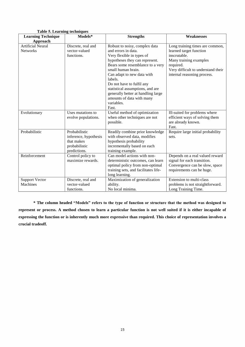
There currently seem to be five popular classes of techniques or mathematical methods in robot
learning: 1) neural method; 2) evolutionary method; 3) reinforcement learning method; 4) probabilistic
method and 5) support vector machines method. There have been significant advances in several of the
underlying technologies, e.g., support vector machines [Cristianini and Shawe-Taylor, 2000]; improved
links between reinforcement learning and stochastic control theory [Bertsekas and Tsitsiklis, 1996];
advances in planning and learning methods for stochastic environments [Littamn, 1996; Parr, 1998]; and
improved theoretical models of simple genetic algorithms [Vose, 1999]. Major types of learning
techniques are summarized in Table 5 [Zimmerman and Kambhampati, 2001; Nordlander, 2001].
23
Table 5. Learning techniques
Learning Technique
Approach
Models* Strengths Weaknesses
Artificial Neural
Networks
Discrete, real and
vector-valued
functions.
Robust to noisy, complex data
and errors in data.
Very flexible in types of
hypotheses they can represent.
Bears some resemblance to a very
small human brain.
Can adapt to new data with
labels.
Do not have to fulfil any
statistical assumptions, and are
generally better at handling large
amounts of data with many
variables.
Fast.
Long training times are common,
learned target function
inscrutable.
Many training examples
required.
Very difficult to understand their
internal reasoning process.
Evolutionary Uses mutations to
evolve populations.
Useful method of optimization
when other techniques are not
possible.
Ill-suited for problems where
efficient ways of solving them
are already known.
Fast.
Probabilistic Probabilistic
inference, hypothesis
that makes
probabilistic
predictions.
Readily combine prior knowledge
with observed data, modifies
hypothesis probability
incrementally based on each
training example.
Require large initial probability
sets.
Reinforcement Control policy to
maximize rewards.
Can model actions with non-
deterministic outcomes, can learn
optimal policy from non-optimal
training sets, and facilitates life-
long learning.
Depends on a real valued reward
signal for each transition.
Convergence can be slow, space
requirements can be huge.
Support Vector
Machines
Discrete, real and
vector-valued
functions.
Maximization of generalization
ability.
No local minima.
Extension to multi-class
problems is not straightforward.
Long Training Time.
* The column headed “Models” refers to the type of function or structure that the method was designed to
represent or process. A method chosen to learn a particular function is not well suited if it is either incapable of
expressing the function or is inherently much more expressive than required. This choice of representation involves a
crucial tradeoff.

24
4 Research methodology
4.1 Problem definition and notation
Notation
Let R be a robot, O an object, and E an environment. This will define the system represented
by ],,[ EOR . Let F be a set of features or patterns representing the physical state of . Let be a
mapping from to F . T is a task performed on O , using R , within the environment E to meet a
goal G . The performance of the task T is a function of a set actions, A , for each physical state of .
The state of the system represented by F will be denoted as S . Let a policy P be a set of state-action
pairs, },{ AS . Let the performance measure be ),( PFZ .
Goal
The goal, G , is to classify a bag correctly, grab it successfully and empty its contents on a
collection container in minimum time.
Task
The task, T , is to observe the position of an unknown bag (e.g., plastic bag, briefcase, backpack,
or suitcase) located on a platform, grasp it with a robot manipulator and shake out its contents on a table
or into a nearby container. It is assumed that all clasps, zippers and locks have already been opened.
Another possible option is to combine both actions of gradually dragging and raising of a bag without
the need to shake it. The system starts with no knowledge about classifications of bags. New bag types
are adaptively learned over time. It has no a-priori knowledge regarding to efficient grasping and
shaking policies. The system learns this knowledge from experience and from human guidance.
System
Robot
The “A255” robot, R , manufactured by “CRS Robotics” is an articulated robotic arm, with five
degrees of freedom (X, Y, Z, and orientation, Pitch, and Roll). The “A255” robot system consists of a
robot arm and controller, which runs “RAPL-II” operating software.
Object
The system will contain different types of bags (examples - Figure 1). Different geometrical
attributes will be defined for each bag, O (section 4.4.1). The conclusion about the identity of O , can
take these terms: {plastic bag, briefcase, backpack, suitcase, not recognized, new type}.
Environment
The robotic environment, E , contains a platform on which the inspected bag is manipulated,
light sources, and extraneous objects such as undesirable human hand.

25
(a) Plastic bag (b) Backpack
(c) Soft briefcase (d) Hand briefcase
Figure 1. Different kinds of bags
Features
Let F be a set of features or patterns representing the state of . F may include bag
classifications, robot position and orientation and environmental conditions.
Mapping
Let be visual mapping function which obtains visual image I taken of ],,[ EOR and
extracts a set of representative features of I denoted as F .
Actions
Actions, A , are command instructions such as grasping, shaking, etc.
Policy
Carrying out the task involves a policy P . Given F of ],,[ EOR , a policy )},{( AFP is a
set of state-action pairs.

26
4.2 Performance measures
The performance measures, ),( PFZ , include (Table 6 in section 4.3.2):
1) Classification accuracy.
2) Whether a bag was grabbed successfully or not.
3) Quality - how empty the bag is.
4) Time to completely empty the contents of a bag.
5) Abort task rate.
4.3 Methodology
4.3.1 System architecture
The system architecture (Figure 2) consists of state-action classifiers that receive inputs from a
vision system, a robotic system and a virtual reality (VR) interface.
Figure 2. System architecture
When the state-action classifiers have little or no knowledge about how to proceed on a task,
they can try to obtain that knowledge through advice from the human operator (HO). This is done by
human-robot collaboration in such a way that the HO can affect and change parameters in the learning
algorithms on-line through the VR interface (e.g., by changing the learning rate of the reinforcement
learning (RL) algorithm, suggesting new actions such as shaking plans, intervene in case of
misclassification).
Human
Operator
VR
Interface
State-Action
Classifiers
CameraRobotic
Environment
27
In the proposed system, the search space in which to discover a successful solution may be quite
large. To make this search tractable, the system should accept advice from the HO through its search.
This requires the ability to identify when knowledge is needed as well as to provide the necessary
problem-solving context for the HO so that supplying the knowledge is easy. It must also be possible for
the system to proceed without advice when the HO is unavailable. If guidance is available, the system
will utilize its own strategies together with advice to quickly construct a solution.
In the proposed machine learning framework, two learning classification methods will be used
and compared: 1) On-line adaptive resonance theory (ART) and 2) Off-line support vector machines
(SVMs). The methods will be tested separately and independently from each other (one can treat it as
two “Human-Robot Collaborative Learning systems”).

28
4.3.2 System flow and operational stages
The system operational stages has multiple stages summarized in Table 6.
Table 6. System operational stages
Stage Description Success Failure Human
Intervention
Performance
Measure(s)
Classification Determine the state of the
system ( F ) using visual
and possibly tactile
sensors. This may involve
positioning a robot on
board camera (“hand-in-
eye”) to view the object
position and the
surrounding environment.
It may also involve
touching the object with a
tactile sensor to assess its
composition (soft cloth,
plastic, hard plastic, etc.).
Classification is performed
by image processing
combined with one of the
following: adaptive
resonance theory (ART) or
support vector machines
(SVMs).
A bag was
classified
correctly.
Required for
avoiding the
object
repositioning
stage.
Required for setup -
put manually
various bags on the
robot workspace.
If failure occurs, HO
gives correct
classification.
Classification
accuracy.
Grasping The robot grasps the
object.
A bag was
grasped
successfully.
If a bag was
not grasped at
all.
HO gives a correct
set of possible
grasping points.
Whether a bag
was grasped
successfully or
not.
Object
Repositioning
Re-arranging the position
of the object to prepare it
for easier grasping.
A bag was
grasped
successfully.
If a bag was
not grasped at
all.
HO repeats this
stage until the object
is grasped
successfully.
Whether a bag
was grasped
successfully or
not.
Lift and
shake
The robot lifts the object
above the table or above a
collection container and
shakes out its contents.
Always
successful.
- - -
Verification The system tries to verify
if all the contents have
been extracted.
1) If the
number of
items fell from
a bag is less
than a pre-
determined
threshold for a
shaking policy.
2) Time to
empty the
content of a
bag is less than
a
predetermined
threshold.
1) Not
enough items
fell out.
2) Time to
empty the
contents is
too slow.
3) Abort task
rate is too
high.
1) Suggest new
grasping points
through VR
interface.
2) Suggest new
lifting and shaking
policies through VR
interface.
1) Quality -
how empty the
bag is.
2) Time to
completely
empty the
contents of a
bag.
3) Abort task
rate.
29
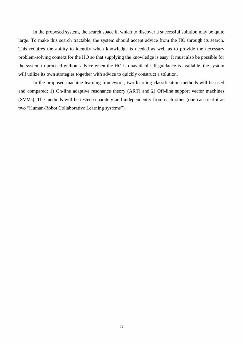
The system flow diagram is shown in Figure 3.
Figure 3. System flow diagram
Acquire New
Bag Image
Identify
Existence of a
Handle
Start
Remove Handle
from Image
Find a Vector
that Represents
the Bag
Handle was
Identified?
Yes No
Is the Handle
Symmetric with
the Bag?
Yes No
Find Bag
Opening
Find Possible
Grasping Points Use ART for
Classifying the
Bag (On-Line
Learning)
Determine Manually
an Area of Possible
Grasping Points
Attach Possible
Grasping Points into
Category (Off-Line
Learning)
Use Reinforcement
Learning Algorithm
for Finding the
Optimal Policy: Best
Starting Grasping
Point, Lift and
Shake Parameters
Remove Handle
from Image
Was a New
Category
Recognized?
Yes No
Verification
Use SVM for
Classifying the
Bag (Off-Line
Learning)
Use only
one
method
Perform Object
Repositioning if
necessary
Performance
Measures

31
The below procedure summarizes the system flow. That includes whether using a learning
method (adaptive resonance theory (ART) or support vector machines (SVMs)) or just use image
processing methods. The reinforcement learning (RL) is also described and is and inseparable of
whether there is learning or not.
4.4 Procedures
The objective is to implement an intelligent system for recognition and classification of bag
shaking learning algorithms through a virtual reality (VR) interface. Three methods will be applied: 1)
adaptive resonance theory; 2) support vector machines and 3) reinforcement learning. The first two will
serve as input module to the reinforcement learning algorithm which will be used for finding the best
For each bag presented to the system, perform as follows:
1) Image processing:
a) Identify the existence of a handle (look at section 4.4.1 for more details).
i) If handle identified, find whether its location is symmetric with the bag.
b) Find the seven parameters vector that represent a bag (after removing handle using image processing
operations) described in section 4.4.1.
2) Learning algorithm:
a) If a handle was identified and symmetric with the bag:
Find the opening of the bag and a set, gpS , of possible grasping points using image processing methods (it is
assumed that points that are far from the opening are better than those that are near).
b) If a handle was not identified or if it was identified, but its location is not symmetric with the bag (that means
that possible grasping points will be found to be wrong) do one of both:
i) Feed an ART neural network on-line with a binary vector representing the bag (details in section 4.4.2)
the seven parameters vector found in 1(b) to classify the bag into categories,
...},,,{: typenewbagplasticsuitcasebriefcaseCb .
ii) Feed SVM off-line with the seven parameters vector found in 1(b) (details in section 4.4.3) to classify
the bag into categories, ,...},,{: bagplasticsuitcasebriefcaseCb .
c) For a bag category found in 2(b) and in which no possible grasping points were found due to image processing
methods, determine manually an area of possible grasping points, gpS .
(d) Attach gpS to bC .
(e) Use reinforcement learning (e.g., Q-learning): Based on a learning function that contains Q-values and system
performance measures described in section 4.2, an optimal policy that includes a starting grasping point, lift and
shake parameters will be determined. It is noted that manual repositioning might be necessary for re-grasping the
bag. Further details are in section 4.4.4.

31
actions (e.g., determining the optimal grasping point followed by a lift and shake trajectory) for a given
state.
4.4.1 Image processing
Processing starts with a grabbed 24-bit color image of a scene. Various image processing
operations are used; conversion to gray-scale, removal of noise from the image due to optical distortions
of the lens, adaptation to ambient and external lighting conditions, and segmentation of the bag from the
background. },,{ EoR SSSS is defined as the state of the system, where RS is the state of the robot, oS
is the state of the bag and ES is the state of the environment (details in section 4.1). For segmenting a
bag, the robot should be at the home position state and no obstructions such as unknown objects (e.g.,
human hand) and bad lighting conditions (e.g., extreme darkness) should exist in the scene. The end
result is an image of segmented bag from which features are extracted. For each bag, the existence of a
handle will be determined (based on finding the image contour and its associative euler number). If a
handle exists, two intersection coordinates (or more, if handle is folded several times) between the
handle and the bag will be found (based on neighboring pixels operations). According to the
intersections found, a recommendation of a set of grasping points will be determined (points exist far
from the handle are better than those which are near) and will be serve as an input to a reinforcement
learning (RL) algorithm that will be described in section 4.4.4.
The next stage will be to separate the bag from its handle (if it exists) using a sequence of erode
and dilate operations (example - Figure 4).
Figure 4. Separating handle from bag example
Each bag (without its handle) will be assigned a vector that consists of seven geometrical
attributes: 1) Area - actual number of pixels in the region; 2) Centroid - coordinates of the center of mass
of the region; 3) Bounding box - the smallest rectangle that can contain the region; 4) Major axis length
- the length of the major axis of the ellipse that has the same second-moments as the region; 5) Minor

32
axis length - the length of the minor axis of the ellipse that has the same second-moments as the region;
6) Eccentricity - the eccentricity of the ellipse that has the same second-moments as the region. The
eccentricity is the ratio of the distance between the foci of the ellipse and its major axis length and 7)
Orientation - the angle between the x-axis and the major axis of the ellipse that has the same second-
moments as the region.
4.4.2 Adaptive resonance theory
The ART-1 unsupervised neural network will be used for clustering binary input vectors (details
are in Appendix VI). Figure 5 describes the inputs and outputs of the ART-1 classification methodology.
Bag image evoked into an image processing module which its output represents a binary vector (pattern)
as described later in this section. The image features produced by the image processing will serve as an
input to an ART-1 module. The output will be a classification to bag categories (e.g., plastic bag,
briefcase, backpack, suitcase, not recognized, new type).
Figure 5. ART-1 architecture methodology
In the proposed algorithm, each bag image captured will be presented as a binary vector that will serve
as input to an ART-1 neural network. The proposed methodology suggests to represent the bag images
in such a way, to avoid the disadvantages of using of the ART-2 network (Appendix VI) on one hand,
and using the ART-1 network and its advantages on the other hand. Image processing operations such as
background separation, black and white transformations, centroid finding and partitioning to regions are
shown in Figure 6 for a sample bag image.
ART-1Image
Processing
Classification
Inferences
Bag Evoked
Binary Vector
Represents a Bag

33
(a) Original sample bag (b) Black and white image
(c) Centroid and ray of image (d) Portioned image
Figure 6. Image processing operations for a sample bag image
As can be seen, the sample image was divided into 14 portions (a different number can also be chosen),
starting from its centroid to the corners and to equal distances predefined coordinates on the border
(constant angles can also be chosen instead of portions):
)}.480,640(),480,480(
),480,320(),480,160(),480,0(),320,640(),320,0(),160,640(),160,0(),0,640(),0,480(),0,320(),0,160(),0,0{(
For each portion, the ratio between the number of the white pixels and the black pixels is calculated and
is compared to a predefined constant value. If this ratio is above this value, then the binary output bit of
a particular portion is noted as “1”, otherwise, it is “0”. Results for the below sample bag image shown
in Figure 7 are shown in Table 7. The constant and tunable value was chosen to be as 1.5, that yields an
input vector }]1,0{[ iss of }11110000011011{:s that represents the bag and will serve the ART-1
network for finding similarity and to classify the bag into its category. The ART-1 learning algorithm
notation, description and comments is described in details in Appendix VI.

34
10841 Pixels
Figure 7. An example for one image portion (noted as region 8) - the black pixels are shown in
yellow and the white pixels are shown in green Table 7. Bag sample example analysis
Region Number of
Black Pixels
Number of
White Pixels
Ratio Binary
Output Bit 1 4623 15598 3.37 1
2 7188 12886 1.79 1
3 8255 11735 1.42 0
4 7339 12714 1.73 1
5 8674 13468 1.55 1
6 9861 12103 1.23 0
7 8940 12569 1.41 0
8 7533 10841 1.44 0
9 8619 9482 1.10 0
10 7820 10594 1.35 0
11 5272 13143 2.49 1
12 7347 21709 2.95 1
13 9962 19042 1.91 1
14 6948 22225 3.20 1
7533 Pixels
1
2 3
4
5
6
7
9 11
11
12
13
14
8
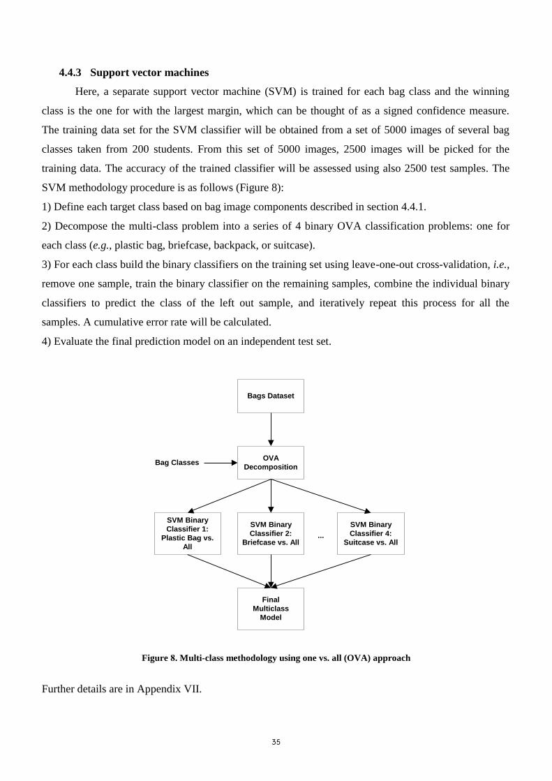
35
4.4.3 Support vector machines
Here, a separate support vector machine (SVM) is trained for each bag class and the winning
class is the one for with the largest margin, which can be thought of as a signed confidence measure.
The training data set for the SVM classifier will be obtained from a set of 5000 images of several bag
classes taken from 200 students. From this set of 5000 images, 2500 images will be picked for the
training data. The accuracy of the trained classifier will be assessed using also 2500 test samples. The
SVM methodology procedure is as follows (Figure 8):
1) Define each target class based on bag image components described in section 4.4.1.
2) Decompose the multi-class problem into a series of 4 binary OVA classification problems: one for
each class (e.g., plastic bag, briefcase, backpack, or suitcase).
3) For each class build the binary classifiers on the training set using leave-one-out cross-validation, i.e.,
remove one sample, train the binary classifier on the remaining samples, combine the individual binary
classifiers to predict the class of the left out sample, and iteratively repeat this process for all the
samples. A cumulative error rate will be calculated.
4) Evaluate the final prediction model on an independent test set.
Figure 8. Multi-class methodology using one vs. all (OVA) approach
Further details are in Appendix VII.
Bags Dataset
OVA
Decomposition
SVM Binary
Classifier 1:
Plastic Bag vs.
All
SVM Binary
Classifier 2:
Briefcase vs. All
SVM Binary
Classifier 4:
Suitcase vs. All
Bag Classes
...
Final
Multiclass
Model
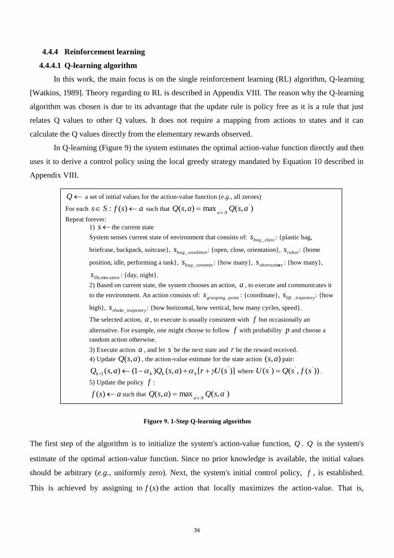
36
4.4.4 Reinforcement learning
4.4.4.1 Q-learning algorithm
In this work, the main focus is on the single reinforcement learning (RL) algorithm, Q-learning
[Watkins, 1989]. Theory regarding to RL is described in Appendix VIII. The reason why the Q-learning
algorithm was chosen is due to its advantage that the update rule is policy free as it is a rule that just
relates Q values to other Q values. It does not require a mapping from actions to states and it can
calculate the Q values directly from the elementary rewards observed.
In Q-learning (Figure 9) the system estimates the optimal action-value function directly and then
uses it to derive a control policy using the local greedy strategy mandated by Equation 10 described in
Appendix VIII.
Figure 9. 1-Step Q-learning algorithm
The first step of the algorithm is to initialize the system's action-value function, Q . Q is the system's
estimate of the optimal action-value function. Since no prior knowledge is available, the initial values
should be arbitrary (e.g., uniformly zero). Next, the system's initial control policy, f , is established.
This is achieved by assigning to )(sf the action that locally maximizes the action-value. That is,
Q a set of initial values for the action-value function (e.g., all zeroes)
For each asfSs )(: such that ),(max),( '' asQasQ
Aa
Repeat forever:
1) s the current state
System senses current state of environment that consists of: classbags _ : {plastic bag,
briefcase, backpack, suitcase}, conditionbags _ : {open, close, orientation}, robots : {home
position, idle, performing a task}, contentsbags _ : {how many}, nsobstructios : {how many},
ationillus min : {day, night}.
2) Based on current state, the system chooses an action, a , to execute and communicates it
to the environment. An action consists of: int_ pograspings : {coordinate}, trajectorylifts _ : {how
high}, trajectoryshakes _ : {how horizontal, how vertical, how many cycles, speed}.
The selected action, a , to execute is usually consistent with f but occasionally an
alternative. For example, one might choose to follow f with probability p and choose a
random action otherwise.
3) Execute action a , and let 's be the next state and r be the reward received.
4) Update ),( asQ , the action-value estimate for the state action ),( as pair:
)]([),()1(),( '
1 sUrasQasQ kkkk where ))(,()( ''' sfsQsU .
5) Update the policy f :
asf )( such that ),(max),( '' asQasQ
Aa

37
asf )( such that ),(max),( '
'asQasQ
Aa where ties are broken arbitrarily. The robot then enters a
cycle of acting and policy updating.
First, the robot senses the current state, },,{ EoR SSSS where RS is the state of the robot, oS is
the state of the object and ES is the state of the environment. RS contains the home position, idle, and
performing a task. The oS state contains the bag class (e.g., plastic bag, briefcase, backpack, suitcase)
and its condition (e.g., open, close, orientation) and ES contains the environmental conditions, such as
how many obstructions are in the scene and illumination (e.g., day or night). It then selects an action A
to perform next. An action consists of a set of coordinates of possible grasping points, lift trajectories
(e.g., manipulate the robotic arm 60cm above the collection container and with 30 degrees left) and
shaking trajectories (e.g., manipulate the robotic arm 10cm horizontally and 15cm vertically in 3m/s
speed for 5 cycles). Most of the time, this action will be the action specified by the system's policy
)(sf , but occasionally the system will choose a random action (choosing an action at random is a
particularly simple mechanism for exploring the environment). Exploration is necessary to guarantee
that the system will eventually learn an optimal policy. The system performs the selected action and
notes the immediate reward r and the resulting state 's . The reward function is probabilistic and
depends on the number of items fell from a bag during lift and shaking operations. The action-value
estimate for the state-action pair ),( as is then updated. Mathematical modeling of the robot-
environment interaction is described in Appendix VIII.
4.5 Testing and validation
4.5.1 Physical experimental setup
In this work, a 5 degrees of freedom (DOF) articulated robot is controlled through a virtual
reality (VR) interface from a remote site for performing various tasks (Figure 10).
Figure 11. Experimental setup
38
The implementation of this work is a client-server application. The server contains a dual frame grabber
connected to stereo cameras mounted over the workspace. Robot control software is also located in the
server. Two additional universal serial bus (USB) cameras are mounted over the workspace for visual
feedback of the scene to the human operator (HO), (the client). From the client site, the HO can take
control over the robot through a VR interface.
4.5.2 Performance evaluation
Three hypotheses will be evaluated:
1) Whether system learning performance increases by human intervention.
2) Whether system performance increases by on-line learning.
3) Whether support vector machines (SVMs) methodology is better than adaptive resonance theory
(ART) for classification. SVMs and ART will be tested separately and independently from each
other (one can treat it as two “Human-Robot Collaborative Learning Systems”). Currently, no other
systems compare between SVMs and ART.
System performance will be evaluated by several independent measures:
1) Speed of convergence to optimality [Kaelbling et al., 1996]. Optimality is usually an asymptotic
result, and so convergence speed is an ill-defined measure. More practical is the speed of
convergence to near-optimality. This measure begs the definition of how near to optimality is
sufficient. A related measure is the level of performance (e.g., whether a bag was classified
correctly, whether a bag was grabbed successfully, how empty the bag is) after a given time, which
similarly requires that someone define the given time. Measures related to speed of learning have an
additional weakness. An algorithm that merely tries to achieve optimality as fast as possible may
incur unnecessarily large penalties during the learning period. A less aggressive strategy taking
longer to achieve optimality, but gaining greater total reinforcement during its learning might be
preferable.
2) Regret. The regret is calculated as the difference between the expected total reward gained by
following a learning algorithm and expected total reward one could gain by playing for the
maximum expected reward from the start [Berry and Fristedt, 1985].
3) Recall ( R )- the percentage of the bags for a given category that are classified correctly, Precision
( P ) - the percentage of the predicted bags for a given category that are classified correctly. It is a
normal practice to combine recall and precision in some way so that classifiers can be compared in
terms of a single rating. 1F rating is one of the commonly used measures, which is defined as
39
)(
21
PR
RPF
[Yang and Liu, 1999]. These scores are calculated for a series of binary classification
experiments, one for each category [He et al., 2000].
4) The ability of the classifiers to generalize will be tested (calculated based on generalization error).
The test will evaluate how well they can observe a new set of system features F and determine the
correct classification.
5 Research plan
5.1 Research stages
The research consists of the following main stages:
1) Application Description:
a) Definition of system performance measures. This includes features that represent the system:
fixed (e.g., robot capabilities, camera features, sensor specifications) and controllable parameters
(e.g., shaking a bag - number of items fell from a bag, robot gripper height, vertical and horizontal
amplitudes in shaking policies).
b) Definition of a representable set of bags. A bag is classified based by the following
characteristics: 1) Bag type (e.g., plastic bag, briefcase, backpack, or suitcase); 2) Bag
specifications (e.g., height, width and depth).
2) Preparation of the VR interface:
a) Implementation of a telerobotic system controlled from VR using “Alice”.
b) Implementing the VR robotic environment in “OpenGL” (replacing “Alice”). This includes
incorporating of kinematic equations for solving the forward / inverse kinematics problem, and
necessary constraints.
c) Design a transformation matrix for mapping the VR to the real world coordinates.
3) Finding a set of points located on the contour of a bag image which some of them are candidates for
grasping using image processing methods. In future steps, the system learns to recognize where a
bag opening is.
4) Studying and implementing training process for classifying several kinds of bags using adaptive
resonance theory (on-line) and support vector machines (off-line) and compare between them based
on several task cases.
5) Design of a set of evacuating policies (state-action pairs).
6) Finding preferable grasping points using reinforcement learning. This includes mathematical
definition of a policy, a reward function, and a value function. This includes also gathering data

41
manually and updating the algorithm functions accordingly and manually positioning of a bag. The
goal is to demonstrate improving performance in learning to find preferable grasping points from a
given set. In this way the system learns to recognize where a bag opening is. Another goal is to learn
which evacuating policy to choose.
7) Determining when HO intervention is required or if the system can behave autonomously when an
unknown event or error occurs. Show how human intervention can provide guidance to improve
overall task performance.
8) Operational system.
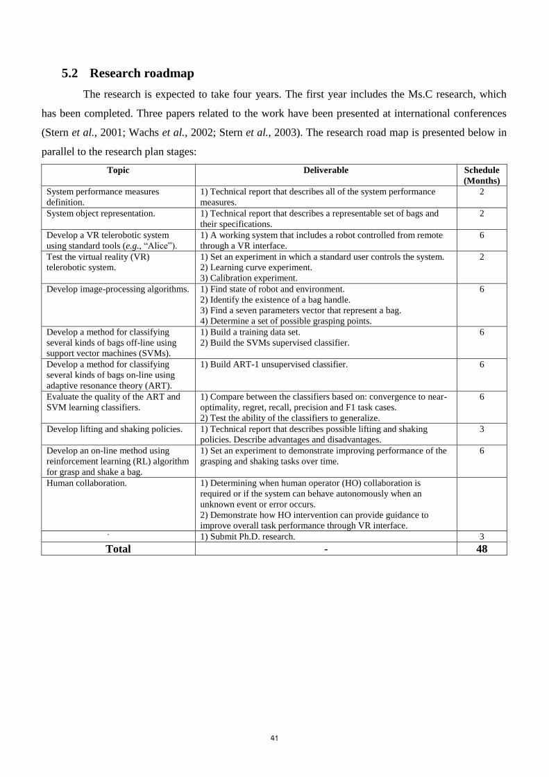
41
5.2 Research roadmap
The research is expected to take four years. The first year includes the Ms.C research, which
has been completed. Three papers related to the work have been presented at international conferences
(Stern et al., 2001; Wachs et al., 2002; Stern et al., 2003). The research road map is presented below in
parallel to the research plan stages:
Topic Deliverable Schedule
(Months)
System performance measures
definition.
1) Technical report that describes all of the system performance
measures.
2
System object representation. 1) Technical report that describes a representable set of bags and
their specifications.
2
Develop a VR telerobotic system
using standard tools (e.g., “Alice”).
1) A working system that includes a robot controlled from remote
through a VR interface.
6
Test the virtual reality (VR)
telerobotic system.
1) Set an experiment in which a standard user controls the system.
2) Learning curve experiment.
3) Calibration experiment.
2
Develop image-processing algorithms. 1) Find state of robot and environment.
2) Identify the existence of a bag handle.
3) Find a seven parameters vector that represent a bag.
4) Determine a set of possible grasping points.
6
Develop a method for classifying
several kinds of bags off-line using
support vector machines (SVMs).
1) Build a training data set.
2) Build the SVMs supervised classifier.
6
Develop a method for classifying
several kinds of bags on-line using
adaptive resonance theory (ART).
1) Build ART-1 unsupervised classifier. 6
Evaluate the quality of the ART and
SVM learning classifiers.
1) Compare between the classifiers based on: convergence to near-
optimality, regret, recall, precision and F1 task cases.
2) Test the ability of the classifiers to generalize.
6
Develop lifting and shaking policies. 1) Technical report that describes possible lifting and shaking
policies. Describe advantages and disadvantages.
3
Develop an on-line method using
reinforcement learning (RL) algorithm
for grasp and shake a bag.
1) Set an experiment to demonstrate improving performance of the
grasping and shaking tasks over time.
6
Human collaboration. 1) Determining when human operator (HO) collaboration is
required or if the system can behave autonomously when an
unknown event or error occurs.
2) Demonstrate how HO intervention can provide guidance to
improve overall task performance through VR interface.
- 1) Submit Ph.D. research. 3
Total - 48
42
6 Ms.C. Thesis - Virtual Reality Telerobotic System
6.1 Introduction
6.1.1 Description of the problem
Teleoperation and telerobotics are technologies that support physical action at a distance. This
distance could span a few yards through a radioactivity proof wall, or millions of miles through a
vacuum to another planet [Goldberg, 2000]. In this work, a virtual reality (VR) telerobotic system was
built using the Internet as the communication link. In today’s world the Internet plays an important role
in everyone’s lives. It provides a convenient way for receiving information, electronic communication,
entertainment and conducting business [Ho and Zhang, 1999]. Robotics researchers are now using the
Internet as a tool to provide feedback for teleoperation [Sheridan, 1992]. Internet-based teleoperation
will inevitably lead to many useful applications in various sectors of society [Ho and Zhang, 1999]. To
understand the meaning of teleoperation, the definition of robotics is examined first. Robotics is the
science of designing and using robots. A robot is defined as “a re-programmable multi-functional
manipulator designed to move materials, parts, tools or specialized devices through variable
programmed motions for the performance of a variety of tasks” [Robot Institute of America, 1979].
Robots can also react to changes in the environment and take corrective actions to perform their tasks
successfully [Burdea and Coiffet, 1994]. Furthermore, all electromechanical systems, such as toy trains,
may be classified as robots because they manipulate themselves in an environment.
Teleoperation is the direct and continuous human control of a teleoperator [Sheridan, 1992]. A
teleoperator can be any machine that extends a person’s sensing or manipulating capability to a location
remote from that person. In situations where it is impossible to be present at the remote location such as
a minefield, at the bottom of the sea or simply at a distant location, a teleoperator can be used instead.
Hirukawa and Hara, 2000, divide teleoperation systems into two groups, from the viewpoint of
motion command transfer. In the first group, an operator controls directly a real robot and manipulates
an object at a remote site. This group is called a direct type. In the second group an operator plans robot
tasks interactively through a computer simulation of a robot and objects, and the planned motions are
sent to control a remote real robot afterward. This group is called an indirect type. The indirect type has
been developed mainly to cope with time delays.
6.1.2 Objective
The fundamental research objective of this work is to develop and evaluate a VR system for
remote robotic experiments.
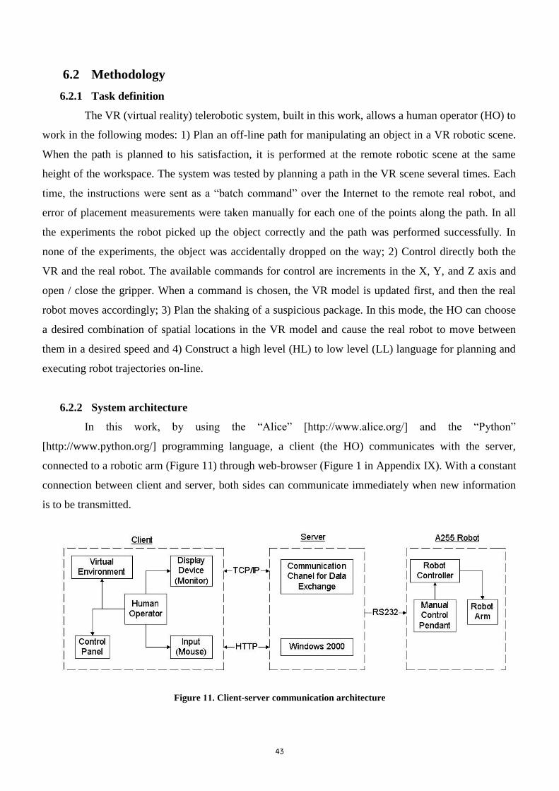
43
6.2 Methodology
6.2.1 Task definition
The VR (virtual reality) telerobotic system, built in this work, allows a human operator (HO) to
work in the following modes: 1) Plan an off-line path for manipulating an object in a VR robotic scene.
When the path is planned to his satisfaction, it is performed at the remote robotic scene at the same
height of the workspace. The system was tested by planning a path in the VR scene several times. Each
time, the instructions were sent as a “batch command” over the Internet to the remote real robot, and
error of placement measurements were taken manually for each one of the points along the path. In all
the experiments the robot picked up the object correctly and the path was performed successfully. In
none of the experiments, the object was accidentally dropped on the way; 2) Control directly both the
VR and the real robot. The available commands for control are increments in the X, Y, and Z axis and
open / close the gripper. When a command is chosen, the VR model is updated first, and then the real
robot moves accordingly; 3) Plan the shaking of a suspicious package. In this mode, the HO can choose
a desired combination of spatial locations in the VR model and cause the real robot to move between
them in a desired speed and 4) Construct a high level (HL) to low level (LL) language for planning and
executing robot trajectories on-line.
6.2.2 System architecture
In this work, by using the “Alice” [http://www.alice.org/] and the “Python”
[http://www.python.org/] programming language, a client (the HO) communicates with the server,
connected to a robotic arm (Figure 11) through web-browser (Figure 1 in Appendix IX). With a constant
connection between client and server, both sides can communicate immediately when new information
is to be transmitted.
Figure 11. Client-server communication architecture

44
Commands sent from the client in the virtual environment (VE) update the VR robot. Through
TCP/IP, the control parameters are sent from the VE to the server via the communication channel.
Another program then extracts them and updates the real robot.
Figure 12. Virtual reality telerobotic system architecture
The following steps were performed for building the system architecture (Figure 12):
1) The robot specifications were achieved: this includes information on the dimensions of the robot, the
limits of movement, the behavior and properties. In addition, information regarding both hardware
and software is essential to allow data exchange between the controller and the robotic environment.
2) Interface techniques and methods of data exchange were determined: a technique of sending and
receiving data to and from the controller was determined to update the robotic variables (e.g. joint
positions, gripper state, etc.) constantly. This information is accessed automatically over the
network. A method of accessing the robotic variables as well as the method of enabling the VR
model to access them were determined. This includes choosing VR software that allows the model to
send and receive data using the same protocol.
Server
Client
Web Camera 2
Web Camera 1
A255 CRS
Robot
Internet Website
Robotic
Environment
C500
Controler
RS
23
2
USB
TC
P/I
P
45
3) A programming language to build the interface was chosen: the language chosen must suit the
purpose of the robotic application and should be able to use the data exchange protocol to
communicate with the robot controller program as well as with the VR model. For controlling and
manipulating these models, “Python” scripts were used.
4) A VR model was built and its behavior was verified: having chosen the right VR tools allows data
exchange in and out of the system. For creating the VE, a rapid prototyping software for creating
interactive 3D was used (“Alice”, http://www.alice.org/). One out of several reasons “Alice” was
chosen, is its ability to import and manipulate 3D models from different software packages, such as
the “3D-Studio-Max” [http://www.discreet.com/].
5) A VR-channel interface was built: having constructed the VR model, codes were then inserted,
enable handshaking and data transfer to and from the interface program.
6) The VR-channel interface was tested until it was error free.
7) The channel-robot interface was built: “RAPL-II” commands sent to the controller enabling this data
exchange. Codes were inserted into the channel program for the same reason.
8) Interfaces were tested with full capability.
9) Full integration was tested.
6.2.3 Tools
The following tools were used for building the virtual reality (VR) telerobotic system: 1)
Personal computer workstation (PC) - the server is a Pentium-4 PC with Microsoft
[http://www.microsoft.com/] Windows 2000 as the operating system (OS). A visual basic (VB) based
web server is running on this host to service incoming network requests. Furthermore, the remote host is
connected to the robot controller and two universal serial bus (USB) cameras; 2) Robot and its controller
- a 5 DOF (degrees of freedom) articulated robot was used as the slave robot. The manufacturer provides
the controller for the robot that is connected to the remote host machine through serial cable; 3) Web
cameras - two 3Com [http://www.3com.com/] “HomeConnect” web cameras are used as the video
cameras to observe the robotic environment. “HomeConnect” was chosen because of its low cost and its
ability to be adapted to any PC by simply plug-and-play into a USB port. No extra image capturing is
required. The image capturing software, “Webcam32” [Kolban D., 1998] is provided by the
manufacturer and runs on the remote host machine. It captures images, which are 240X180 pixels in 24
bit colors. By using two web-cameras and the “Webcam32”, live images are constantly being sent and
update the remote client. The USB protocol allows connecting up to 127 devices to a computer. Each
device can consume up to a maximum of 6 megabits per second of network bandwidth.

46
When a user enters the system web-site, predefined characteristically images are being sent to
his web-browser (close and general views in Figure 1 in appendix IX). “Webcam32” supports two types
of direct image delivery. The first, called “Single Frame” sends once, a single frame. The second, called
the “Server-Push” provides a stream of frames that is constantly being sent to web-browsers and
provides real-time update as processor speed and bandwidth allow.
6.2.4 Physical Description of the System
The articulated robot arm, “A255”, manufactured by “CRS Robotics”
[http://www.crsrobotics.com/] was used in this work. The “A255” robot system consists of robot arm
and robot controller, which runs “RAPL-II” operating software. Programming features include
continuous path, joint interpolation, point-to-point relative motions, and an on-line path planner, to
blend commanded motions in joint or straight-line mode. A gripper was installed on the robot arm to
perform tasks. The arm is articulated with five joints, giving it five degrees of freedom. This allows it to
move a tool to spatial coordinates and orientation defined by X, Y, Z, Pitch, and Roll. An “A255” robot
can be operated with a serial teach pendant, a video display terminal (VDT) with serial I/O, or a PC. The
range of motion of each joint and the length of each section (base, links, or tool flange) defines the
workspace of the “A255” robotic arm.
The “C500” controller is a computerized electronics unit with memory that provides control
signals necessary for the operation of the robot arm. Control signals are issued by the execution of
“RAPL-II” commands stored in the controller’s memory. The “RAPL-II” robot programming language
uses English-like command structures. The “C500” contains control functions required for stand-alone
robot operation and a digital display for full diagnostics. These controls can be duplicated on a remote
panel to provide control if the controller is mounted away from the operator’s station. The serial teach
pendant functions as a remote control that allows manual movement of the robot arm, location teaching,
and other operator programming. It has a four-line, 20-character “LCD” display and a 45-key keypad. Its
safety features include an emergency stop button and a live-man switch. The “C500”’s stored kinematic
solutions provide full robot control in world, tool, and cylindrical programming.
When the power to the controller is off, the arm position data in its memory is lost. As a result,
when the controller is powered on, it does not know the position of the arm. The procedure called
“homing” moves the arm to a factory-installed position, which is permanently retained in the controller
memory. At this position, each joint’s encoder disk is aligned to its zero pulse position. Afterward,
during any motion, the encoders continually send position counts to the controller. Using these counts,
the controller knows any position of the arm relative to the home-position.
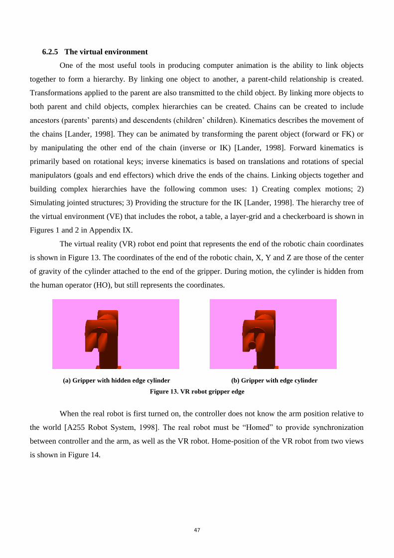
47
6.2.5 The virtual environment
One of the most useful tools in producing computer animation is the ability to link objects
together to form a hierarchy. By linking one object to another, a parent-child relationship is created.
Transformations applied to the parent are also transmitted to the child object. By linking more objects to
both parent and child objects, complex hierarchies can be created. Chains can be created to include
ancestors (parents’ parents) and descendents (children’ children). Kinematics describes the movement of
the chains [Lander, 1998]. They can be animated by transforming the parent object (forward or FK) or
by manipulating the other end of the chain (inverse or IK) [Lander, 1998]. Forward kinematics is
primarily based on rotational keys; inverse kinematics is based on translations and rotations of special
manipulators (goals and end effectors) which drive the ends of the chains. Linking objects together and
building complex hierarchies have the following common uses: 1) Creating complex motions; 2)
Simulating jointed structures; 3) Providing the structure for the IK [Lander, 1998]. The hierarchy tree of
the virtual environment (VE) that includes the robot, a table, a layer-grid and a checkerboard is shown in
Figures 1 and 2 in Appendix IX.
The virtual reality (VR) robot end point that represents the end of the robotic chain coordinates
is shown in Figure 13. The coordinates of the end of the robotic chain, X, Y and Z are those of the center
of gravity of the cylinder attached to the end of the gripper. During motion, the cylinder is hidden from
the human operator (HO), but still represents the coordinates.
(a) Gripper with hidden edge cylinder (b) Gripper with edge cylinder
Figure 13. VR robot gripper edge
When the real robot is first turned on, the controller does not know the arm position relative to
the world [A255 Robot System, 1998]. The real robot must be “Homed” to provide synchronization
between controller and the arm, as well as the VR robot. Home-position of the VR robot from two views
is shown in Figure 14.
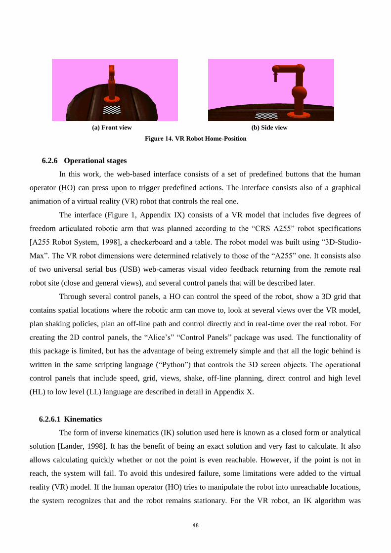
48
(a) Front view (b) Side view
Figure 14. VR Robot Home-Position
6.2.6 Operational stages
In this work, the web-based interface consists of a set of predefined buttons that the human
operator (HO) can press upon to trigger predefined actions. The interface consists also of a graphical
animation of a virtual reality (VR) robot that controls the real one.
The interface (Figure 1, Appendix IX) consists of a VR model that includes five degrees of
freedom articulated robotic arm that was planned according to the “CRS A255” robot specifications
[A255 Robot System, 1998], a checkerboard and a table. The robot model was built using “3D-Studio-
Max”. The VR robot dimensions were determined relatively to those of the “A255” one. It consists also
of two universal serial bus (USB) web-cameras visual video feedback returning from the remote real
robot site (close and general views), and several control panels that will be described later.
Through several control panels, a HO can control the speed of the robot, show a 3D grid that
contains spatial locations where the robotic arm can move to, look at several views over the VR model,
plan shaking policies, plan an off-line path and control directly and in real-time over the real robot. For
creating the 2D control panels, the “Alice’s” “Control Panels” package was used. The functionality of
this package is limited, but has the advantage of being extremely simple and that all the logic behind is
written in the same scripting language (“Python”) that controls the 3D screen objects. The operational
control panels that include speed, grid, views, shake, off-line planning, direct control and high level
(HL) to low level (LL) language are described in detail in Appendix X.
6.2.6.1 Kinematics
The form of inverse kinematics (IK) solution used here is known as a closed form or analytical
solution [Lander, 1998]. It has the benefit of being an exact solution and very fast to calculate. It also
allows calculating quickly whether or not the point is even reachable. However, if the point is not in
reach, the system will fail. To avoid this undesired failure, some limitations were added to the virtual
reality (VR) model. If the human operator (HO) tries to manipulate the robot into unreachable locations,
the system recognizes that and the robot remains stationary. For the VR robot, an IK algorithm was

49
implemented to determine the joint angles required reaching a specific spatial location by supplying the
X, Y and Z coordinates. Further details appear in Appendix XI.
The VR and the real worlds are different from each other by the position, orientation, and
scaling of the robots, the checkerboards and the objects. Therefore, a transformation matrix was
calculated. The transformation matrix was calculated based on 32 intersection points taken from both the
VR and the real checkerboards. Table 1 that appears in Appendix XII presents the intersection
coordinates taken from both the VR and the real environments. Figures 1 and 2 that appear in Appendix
XII show the real and VR coordinate systems accordingly. This includes necessary lengths and
positions. It is assumed that both the VR and the real robot bases are located at point (0,0). Xvr, Yvr
represent VR values and Xr, Yr represent real values. The transformation matrix (Figures 3 and 4 in
appendix XII) was calculated by using a method for aligning a pair of shapes [Cootes et al., 1992] which
is based on the least-squares approach. More details appear in Appendix XII.
6.3 System test and validation
6.3.1 Calibration
The identified parameters related to robotics calibration are accuracy, repeatability, and
resolution [Conrad et al., 2000]. Each of these depends on the various components used (links, motors,
encoders, etc.), the construction procedure, and the capability of the controller [Conrad et al., 2000].
Resolution is defined as the smallest incremental move that the robot can physically produce [Conrad et
al., 2000]. Repeatability is a measure of the ability of the robot to move back to the same position and
orientation [Conrad et al., 2000]. Accuracy is defined as the ability of the robot to precisely move to a
desired position in 3D space [Conrad et al., 2000].
The calibration experiment performed here starts with manually controlling the virtual reality
(VR) robot arm and taking the coordinates of several points (Xvr, Yvr) that were reported by “Alice”
(Figure 15). These points were inserted into the transformation matrix. The calculated output of the
transformation (Xr, Yr) was sent to the real robot, and compared with corresponding manually measured
coordinates from the real robotic scene.
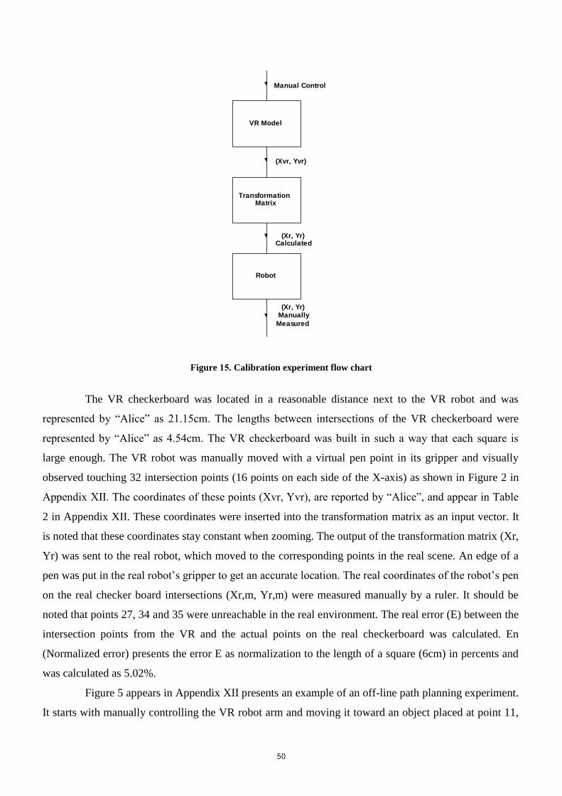
51
VR Model
TransformationMatrix
Robot
Manual Control
(Xr, Yr)Calculated
(Xvr, Yvr)
(Xr, Yr)Manually
Measured
Figure 15. Calibration experiment flow chart
The VR checkerboard was located in a reasonable distance next to the VR robot and was
represented by “Alice” as 21.15cm. The lengths between intersections of the VR checkerboard were
represented by “Alice” as 4.54cm. The VR checkerboard was built in such a way that each square is
large enough. The VR robot was manually moved with a virtual pen point in its gripper and visually
observed touching 32 intersection points (16 points on each side of the X-axis) as shown in Figure 2 in
Appendix XII. The coordinates of these points (Xvr, Yvr), are reported by “Alice”, and appear in Table
2 in Appendix XII. These coordinates were inserted into the transformation matrix as an input vector. It
is noted that these coordinates stay constant when zooming. The output of the transformation matrix (Xr,
Yr) was sent to the real robot, which moved to the corresponding points in the real scene. An edge of a
pen was put in the real robot’s gripper to get an accurate location. The real coordinates of the robot’s pen
on the real checker board intersections (Xr,m, Yr,m) were measured manually by a ruler. It should be
noted that points 27, 34 and 35 were unreachable in the real environment. The real error (E) between the
intersection points from the VR and the actual points on the real checkerboard was calculated. En
(Normalized error) presents the error E as normalization to the length of a square (6cm) in percents and
was calculated as 5.02%.
Figure 5 appears in Appendix XII presents an example of an off-line path planning experiment.
It starts with manually controlling the VR robot arm and moving it toward an object placed at point 11,

51
then it is picked up and moved along a path to touch point 22 and finally it is dropped at point 7. Figure
6 in Appendix XII presents the flow chart of this example. When the path is planned to the human
operator’s (HO's) satisfaction, it is performed in the remote real robotic scene. The measurements are
shown in Table 3 in Appendix XII. The real error (E) between the measured intersection points from the
real scene and the actual points on the real checkerboard was calculated for points 11, 22, and 7. En
(Normalized error) presents the error E as normalization to the length of a square (6cm) in percents and
was calculated as 1.32%.
A repeatability test was set up to measure how precisely the robot can return to the same
position. The robot arm was instructed to move from point 0 to an arbitrary point (16) shown in Figure 7
in Appendix XII several times in the real environment. The motions lead to differing displacements. 10
measurements were taken and reported from the robot controller as shown in Table 4 in Appendix XII.
In each one of the measurements, the gripper was moved manually as close as possible to point 0 which
its accurate coordinates are (265, -240) mm from the robot origin, then it was moved 60mm in the X
axis and 420mm in the Y axis to point 16. Each time the coordinates of point 16 were taken, and the
distance between the points was calculated. The repeatability is defined as the difference between the
maximum and the minimum between point 0 and 16 of the 10 measurements was found to be 0.1260mm
whereas according to the manufacturer specifications it should be 0.05mm.
6.3.2 System learning curve experiment
An experiment was performed in which a human operator (HO) using the virtual reality (VR)
model and its interface controls the remote robot to empty the contents of a bag onto the platform
(Figure 16). It is assumed that the contents of the bag are ten identical electronic components and that
the HO knows this number in advance.
Figure 16. “A255” robot, plastic bag, platform and ten electronic components
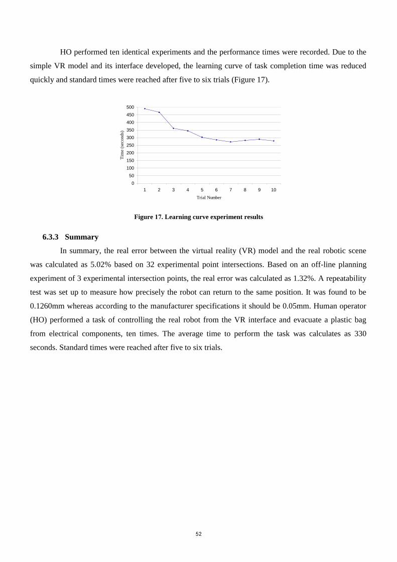
52
HO performed ten identical experiments and the performance times were recorded. Due to the
simple VR model and its interface developed, the learning curve of task completion time was reduced
quickly and standard times were reached after five to six trials (Figure 17).
Figure 17. Learning curve experiment results
6.3.3 Summary
In summary, the real error between the virtual reality (VR) model and the real robotic scene
was calculated as 5.02% based on 32 experimental point intersections. Based on an off-line planning
experiment of 3 experimental intersection points, the real error was calculated as 1.32%. A repeatability
test was set up to measure how precisely the robot can return to the same position. It was found to be
0.1260mm whereas according to the manufacturer specifications it should be 0.05mm. Human operator
(HO) performed a task of controlling the real robot from the VR interface and evacuate a plastic bag
from electrical components, ten times. The average time to perform the task was calculates as 330
seconds. Standard times were reached after five to six trials.
0
50
100
150
200
250
300
350
400
450
500
1 2 3 4 5 6 7 8 9 10
Trial Number
Tim
e (s
eco
nds)
53
7 References
A255 Robot System. 1998. CRS Robotics Human Scale Solutions.
Abe S. 2001. Pattern Classification: Neuro-fuzzy Methods and Their Comparison. Springer-Verlag,
London, UK.
Ackley D. H. and Littman M. L. 1990. Generalization and Scaling in Reinforcement Learning. In D.
S. Touretzky (Ed.), Advances in Neural Information Processing Systems 2. pp. 550-557. CA.
Asoh H., Vlassis N. A., Motomura Y., Asano F., Hara I., Hayamizu S., Ito K., Kurita T., Matsui T.,
Bunschoten R. and Kröse Ben J. A. 2001. Jijo-2: An Office Robot that Communicates and Learns. IEEE
Intelligent Systems. Vol. 16. Num 5. pp. 46-55.
Aycard O. and Washington R. 2000. State Identification for Planetary Rovers: Learning and
Recognition. Proceedings of the IEEE International Conference on Robotics and Automation. pp. 1163-
1168.
Backes P., Tso K., Tharp G. 1998. Mars Pathfinder Mission Internet-based Operations using WITS.
IEEE International Conference on Robotics and Automation.
Balaguer F. and Mangili A. 1991. Virtual Environments, In New Trends in Animation and
Visualization. John Wiley and Sons.
Baltus G., Fox D., Gemperle F., Goetz J., Hirsch T., Magaritis D., Montemerlo M., Pineau J., Roy N.
Schulte J. and Thrun S. 2000. Towards Personal Service Robots for the Elderly. Proceedings of the
Workshop on Interactive Robotics and Entertainment (WIRE). Pittsburgh.
Basu A. Watters C. and Shepherd M. 2003. Support Vector Machines for Text Categorization. 36 th
Annual Hawaii International Conference on System Sciences.
Bertsekas D. P. and Tsitsiklis J. N. 1996. Neuro-Dynamic Programming. Athena Scientific.
Belmont, Massachusetts.
Bhanu B., Leang P., Cowden C., Lin Y. and Patterson M. 2001. Real-Time Robot Learning.
International Conference on Robotics and Automation. Seoul. Korea.
Bellman R. 1957. Dynamic Programming. Princeton University Press.
Berry D. A. and Fristedt B. 1985. Bandit Problems: Sequential Allocation of Experiments. Chapman
and Hall.
Bertsekas D. P. 1987. Dynamic Programming. Deterministic and Stochastic Models. Prentice Hall.
Bertsekas D. P. and Tsitsiklis J. N. 1996. Neuro-Dynamic Programming. Athena Scientific.
Bierbaum and Just. 1998. Course Notes for SIGGRAPH 98 Course 14. Applied Virtual Reality.
Orlando.
54
Board on Army Science and Technology. 2002. Technology Development for Army Unmanned
Ground Vehicles.
Burdea G. 1999. Invited Review: The Synergy between Virtual Reality and Robotics. IEEE
Transactions on Robotics and Automation. Vol. 15. Num. 3. pp. 400-410.
Burdea G. and Coiffet P. 1994. Virtual Reality Technology. John Wiley & Sons Inc.
Cañamero D., Lanzi P. L., Nuttin M. and Wyatt J. 1999. Report on the Eighth European Workshop
on Learning Robots. Ecol´e Polytechnique F´ed´erale de Lausanne. Switzerland.
Carpenter G. A. and Grossberg S. 1987. A Massively Parallel Architecture for a Self Organizing
Neural Pattern Recognition Machine. Computer Vision, Graphics, and Image Processing. Vol. 37. pp.
54-115.
Carpenter G. A. and Grossberg S. 1987. ART2: Self Organization of Stable Category Recognition
Codes for Analog Input Patterns'. Applied Optics. Vol. 26. Num. 23. pp. 4919-4930.
Carpenter G. A. and Grossberg S. 1990 ART3: Hierarchical Search Using Chemical Transmitters in
Self-Organizing Pattern Recognition Architectures. Neural Networks. Vol. 3, pp. 129-152.
Carpenter G. A., Grossberg S. and Rosen D.B. 1991. ART2-A: An Adaptive Resonance Algorithm
for Rapid Category Learning and Recognition. Neural Networks. Vol. 4, pp. 493-504.
Carpenter G. A., Grossberg S. and Reynolds J. H. 1991. ARTMAP: Supervised Real-Time Learning
and Classification of Nonstationary Data by a Self-Organizing Neural Network. Neural Networks. Vol.
4. pp. 565-588.
Carpenter G. A., Grossberg S. and Rosen D. B. 1991. Fuzzy ART: Fast Stable Learning and
Categorization of Analog Patterns by an Adaptive Resonance System. Neural Networks. Vol. 4. pp. 759-
771.
Carpenter G. A., Grossberg S., Markuzon N., Reynolds J. H. and Rosen, D.B. 1992. Fuzzy
ARTMAP: A Neural Network Architecture for Incremental Supervised Learning of Analog
Multidimensional Maps. IEEE Transactions on Neural Networks. Vol. 3. No. 5. pp. 698-713.
Carreras M., Ridao P. Batlle J. and Nicosevici T. 2002. Efficient Learning of Reactive Robot
Behaviors with a Neural-Q Learning Approach. IEEE International Conference on Automation, Quality
and Testing. Romania.
Cao Y. U., Chen T. W., Harris M. D., Kahng A. B., Lewis M. A. and Stechert A. D. 1995. A Remote
Robotics Laboratory on the Internet. INET-95, Honolulu. 65-72.
Cipolla R. and Hollinghurst N. 1997. Visually Guided Grasping in Unstructured Environments.
Journal of Robotics and Autonomous Systems. Vol. 19. Num. 3-4.

55
Clarke R. 1994. Asimov’s Laws of Robotics: Implications for information technology. IEEE
Computer. Vol. 26. Num. 12, Vol. 27. Num. 1.
Connell J. H. and Mahadevan S. 1993. Robot Learning. Kluwer Academic Publishers. Boston.
Conrad K. L. Shiakolas P. S. and Yih T. C. 2000. Proceedings of the 8 th Mediterranean Conference
on Control and Automation.
Conway M. J., Pausch R., Gossweiler R. and Burnette T. 1993. Alice: A Rapid Prototyping System
for Building Virtual Environments. University of Virginia, School of Engineering.
Conway M. J. 1997 Alice: Easy-to-Learn 3D Scripting for Novices. Ph.D. Dissertation.
Cooper S., Dann W. and Pausch R. 2000. Alice: A 3-D Tool for Introductory Programming
Concepts. Proceedings of the 5 th Annual CCSC Northeastern Conference. Ramapo.
Cootes T.F., Taylor C. J., Cooper D. H. and Graham J. 1992. Training Models of Shape from Sets of
Examples. Proceedings of the British Machine Vision Conference.
Cristianini N. and Shawe-Taylor J. 2000. An Introduction to Support Vector Machines: and other
Kernel-Based Learning Methods. Cambridge University Press. England.
Cruz-Neira C. 1995. Virtual Reality Based on Multiple Projection Screens: The CAVE and Its
Applications to Computational Science and Engineering. Ph.D. Dissertation, University of Illinois at
Chicago.
Dann W. Cooper S. and Pausch R. 2000. Making the Connection: Programming With Animated
Small World.
Dietterich T. G. and Bakiri G. 1991. Error Correcting Output Codes: A General Method for
Improving Multiclass Inductive Learning Programs. Proceedings of the Ninth National Conference on
Artificial Intelligence. AAAI Press. pp. 572-577.
Durlach I. N. and Mavor S. N. 1995. Virtual Reality: Scientific and Technological Challenges.
National Academy Press. Washington D.C.
Lund H. H. and Pagliarini L. 2000. Robocup jr. with Lego Mindstorms. Proceedings of International
Conference on Robotics and Automation (ICRA2000).
Holland J. H. 1975. Adaptation in Natural and Artificial Systems. The University of Michigan Press.
Earnshaw R.A., Gigante M.A. and Jones H. 1994. Virtual Reality Systems. Academic Press Limited.
Evgeniou T., Pontil M., Poggio T. 2000. Regularization Networks and Support Vector Machines.
Advances in Computational Mathematics. Vol. 13. pp. 1-50.
Floreano D. and Mondada F. 1996. Evolution of Homing Navigation in a Real Mobile Robot. IEEE
Transactions on Systems, Man, and Cybernetics.

56
Fukuda T. and Kubota N. 1999. An Intelligent Robotic System based on Fuzzy approach.
Proceedings of the IEEE International Conference on Robotics and Automation. Vol. 87. Num. 9. pp.
1448-1470.
Gjerdingen D. 2000. The Use of Machine Learning in Improving Robot Interaction with the
Environment. Proceedings of the Computer Science Discipline Seminar Conference (CSCI 3901).
Goldberg K. 2000. The Robot in the Garden. MIT Press.
Goldberg K., Maschna M. and Gentner S. 1995. Desktop Teleoperation via the WWW. Proceedings
of the IEEE International Conference on Robotics and Automation. pp. 654-659.
Goldberg K. and Santarromana. 1997. About the Tele-Garden.
http://telegarden.aec.at/html/intro.html
Goldenberg A.A., Wiercienski J., Kuzan P., Szymczyk C., Fenton R.G., and Shaver B. 1995. A
Remote Manipulator for Forestry Operation. IEEE Transactions on Robotics and Automation. Vol. 11.
Num. 2. pp. 185-197.
Graefe V. 1995. Object and Behavior-oriented Stereo Vision for Robust and Adaptive Robot
Control. Proceedings of the International Symposium on Microsystems, Intelligent Materials, and
Robots. pp. 560-563.
Grossberg S. 1976. Adaptive Pattern Recognition and Universal Recoding: II. Feedback,
Expectation, Olfaction, and Illusions. Biological Cybernetics. Vol. 23. pp.187-202.
Harvey N.R., Perkins S., Pope P.A., Theiler J., David N.A.and Porter R.B. 2003. Investigation of
Automated Feature Extraction Using Multiple Data Sources. Proceedings of the AEROSENSE. Orlando.
Hastie T. J. and Tibshirani R. J. 1998. Classification by Pairwise Coupling. In Jordan M.I., Kearnsa
M.J., Solla S.A., eds., Advances in Neural Information Processing Systems. MIT Press. Vol. 10.
He J., Tan A-H and Tan C-L. 2000. Machine Learning Methods for Chinese Web page
Categorization. ACL'2000 2 nd Chinese Language Processing Workshop. Hong Kong. pp. 93-100.
Heguy O., Rodriguez N., Luga H., Jessel J. P. and Duthen Y. 2001. Virtual Environment for
Cooperative Assistance in Teleoperation. The 9 th International Conference in Central Europe on
Computer Graphics, Visualization and Computer Vision.
Heisele B., Ho P. and Poggio T. 2001. Face Recognition with Support Vector Machines: Global
Versus Component-based Approach. International Conference on Computer Vision (ICCV'01). Canada.
Vol. 2. pp. 688-694.
Heins L.G. and Tauritz D.R. 1995. Adaptive Resonance Theory (ART): An Introduction.
http://www.cs.brandeis.edu/~cs113/docs/other/heins_tauritz.pdf

57
Ho T. T. and Zhang H. 1999. Proceedings of the 1999 IEEE Canadian Conference on Electrical and
Computer Engineering.
Hine B., Hontalas P., Fong T. W., Piguet L., Nygren E. and Kline A. 1995. VEVI: A Virtual
Environment Teleoperations Interface for Planetary Exploration. SAE 25th International Conference on
Environmental Systems.
Hinton G. E., Rumelhart D. E. and Williams R. J. 1986. Learning Internal Representations by Error
Propagation. In Parallel Distributed Processing, McClelland J.L. and Rumelhart D. E. Eds. MIT Press.
Vol. 1. pp.318-362.
Hirukawa H. and Hara I. 2000. The Web's Top Robotics. IEEE Robotics and Automation Magazine.
Vol. 7. Num. 2.
Hirzinger G., Brunner B., Dietrich J. and Heindl J. 1993. Sensor-Based Space Robotics-ROTEX and
its Telerobotic Features. IEEE Transactions on Robotics and Automation. Vol. 9. Num. 5.
Hsu L., Costa R., Lizarralde F. and Soares J. 1999. Passive Arm Based Dynamic Positioning System
for Remotely Operated Underwater Vehicles. IEEE International Conference on Robotics and
Automation. Vol. 1. pp. 407-412.
http://www.3com.com/
http://www.alice.org/
http://www.crsrobotics.com/
http://www.discreet.com/
http://www.microsoft.com/
http://www.olympus.com/
http://www.opengl.com/
http://www.python.org/
http://www.sega.com/
http://www.sgi.com/
http://www.sony.com/
http://www.telegarden.aec.at/
http://www.telerobot.mech.uwa.edu.au/
http://www.telescope.org/
http://www.usuhs.mil/
Jaakkola T., Jordan M. I. and Singh S. P. 1994. On the Convergence of Stochastic Iterative Dynamic
Programming Algorithms. Neural Computation.
58
Kaelbling L. P., Littman M. L. and Moore A. W. 1996. Reinforcement Learning: A Survey. Journal
of Artificial Intelligence. Vol. 4. pp. 237-285.
Kalawsky R. S. 1993. The Science of Virtual Reality and Virtual Environments. Adison-Welsey
Publishing Company.
Kerr J. and Compton P. 2003. Workshop on Mixed-Initiative Intelligent Systems, International Joint
Conference on Artificial Intelligence. Mexico.
Kim K. I. and Kim J. H. 2002. Face Recognition using Support Vector Machines with Local
Correlation Kernels. International Journal of Pattern Recognition and Artificial Intelligence. Vol. 16.
Num. 1. pp. 197-111.
Kreuziger J. 1992. Application of Machine Learning to Robotics - an Analysis. Proceedings of the
Second International Conference on Automation, Robotics and Computer Vision. Singapore.
Kwon D., Woo K. Y. and Cho H. S. 1999. Haptic Control of the Master Hand Controller for a
Microsurgical Telerobot System. IEEE International Conference on Robotics and Automation.
Lander J. 1998 .Oh My God, I Inverted Kine .Game Developer Magazine.
Längle T., Lüth T. C., Stopp E. and Herzog G. 1996. Natural Language Access to Intelligent Robots:
Explaining Automatic Error Recovery. A. M. Ramsay (ed.), Artificial Intelligence: Methodology,
Systems, Applications. Amsterdam. pp. 259-267.
Lee K. H., Tan H. S. and Lie T. J. 2000. Virtual Operator Interface for Telerobot Control.
Proceedings of the 6 th International Conference on Modern Industrial Training. Beijing. pp. 250-258.
Littamn M. L. 1996. Algorithms for Sequential Decision-Making. Ph.D. Thesis. Brown University.
Lund H. H. and Pagliarini L. 2000. Robocup Jr. with LEGO-Mindstorms. Proceedings of the
International Conference on Robotics and Automation. NJ.
Lutz M. 2001. Programming Python. O'Reilly & Associates.
Macedonia M.R. and Zyda M. J. 1997. A Taxonomy for Networked Virtual Environments. IEEE
Multimedia.
Maes P., Darrell T., Blumberg B. and Pentland A. 1996. The ALIVE System: Wireless, Full-Body
Interaction with Autonomous Agents. ACM Multimedia Systems, Special Issue on Multimedia and
Multisensory Virtual Worlds.
Masterson J. W., Towers R. L. and Fardo S. W. 1996. Robotics Technology. The Goodheart-Willcox
Company.
Meeden L. A. 1996. An Incremental Approach to Developing Intelligent Neural Network
Controllers for Robots. IEEE Transactions on Systems, Man, and Cybernetics , Part B: Cybernetics.
Vol. 26. Num. 3. pp. 474-485.
59
Milgram P., Zhai S. and Drascic D. 1993. Applications of Augmented Reality for Human-Robot
Communication. International Conference on Intelligent Robots and Systems. Japan.
Moghaddam B. and Yang M-H. 2001. Sex with Support Vector Machines. In: Leen T. K., Dietterich
T.G. and Tresp V. (eds): Advances in Neural Information Processing Systems 13. MIT Press,
Cambridge, MA.
Mukherjee S. 2003. Classifying Microarray Data Using Support Vector Machines. In: A Practical
Approach to Microarray Data Analysis, Berrar D. P., Dubitzky W. and Granzow M. (Eds.), Kluwer
Academic Publishers. Vol. 9. pp. 166-185.
Nguyen M. C. 1997. Stereo Vision-Based Robot Control Without Calibration. Proceedings of the
VACETS Technical International Conference.
Nolfi S. 1997. Using Emergent Modularity to Develop Control Systems for Mobile Robots. Adaptive
Behavior, Special Issue on Environment Structure and Behavior. Vol. 5. Num. 3-4. pp. 343-363.
Nolfi S. and Parisi D. 1997. Learning to Adapt to Changing Environments in Evolving Neural
Networks. Adaptive Behavior. Vol. 5. Num. 1. pp. 75-98.
Nordlander T. E. 2001. AI Surveying: Artificial Intelligence in Business. Ms.C in Management
Science. Department of Management Science and Statistics. De Montfort University.
Nourbakhsh I., et al. 1999. An Affective Mobile Robot Educator with a Full-Time Job. Artificial
Intelligence. Vol. 114. Num. 1-2.
Parr. R. 1998. Hierarchical Control and Learning for Markov Decision Processes. Ph.D.
Dissertation. Berkeley.
Preece J., Rogers Y., Sharp H., Benyon D., Holland S. and Carey T. 1994. Human-Computer
Interaction. Adison-Welsey Publishing Company.
Rastogi A., Milgram P. and Grodski J. J. 1995. Augmented Telerobotic Control: a Visual Interface
for Unstructured Environments. University of Toronto and Defense and Civil Institute of Environmental
Medicine.
Rifkin R., Mukherjee S., Tamayo P., Ramaswamy S., Yeang C-H, Angelo M., Reich M., Poggio T.,
Lander E.S., Golub T.R. and Mesirov J.P. 2003. An Analytical Method for Multiclass Molecular Cancer
Classification. SIAM Review (in press).
Robot Institute of America. 1979.
Ross S. M. 1983. Introduction to Stochastic Dynamic Programming. Academic Press.
Rummery G. A. and Niranjan M. 1994. On-line Q-learning using Connectionist Systems. Technical
Report. Cambridge University.
61
Sanz P. J. and Sánchez J. S. 2003. Exploring New Object Recognition Techniques for On-line
Robots. Proceedings of the IASTED International Conference on Robotics and Applications.
Saucy P. and Mondada F.1998. KhepOnTheWeb, an Example of Remote Access to Mobile Robotics
Facilities. IROS.
Scárdua L. A., Reali-Costa A. H. and da Cruz J. J. 2000. Learning to Behave by Environment
Reinforcement. RoboCup-99: Robot Soccer World Cup III. Lecture Notes in Artificial Intelligence.
Berlin. Vol. 1856. pp. 439-449.
Scheffer T. and Joachims T. 1999. Expected Error Analysis for Model Selection. Proceedings of the
International Conference on Machine Learning.
Schilling R. J. 1990. Fundamentals of Robotics Analysis & Control. Prentice Hall.
Sheridan T. B. 1992. Telerobotics, Automation, and Human Supervisory Control. MIT Press.
Sheridan T. B. 1997. Eight Ultimate Challenges of Human-Robot Communication. IEEE
Proceedings of RO-MAN.
Shigeo A. 2001. Support Vector Machines for Pattern Classification. http://frenchblue.scitec.kobe-
u.ac.jp/~abe/pdf/SVMsforPCabs.pdf
Singh S., Jaakkola T., Littman M. L. and Szepesvári C. 2000. Convergence Results for Single-step
On-policy Reinforcement-learning Algorithms. Machine Learning.
Sutton R. S. and Barto A. G. 1998. Reinforcement Learning: An Introduction. MIT Press.
Sutton. R. S. 1996. Generalization in Reinforcement Learning: Successful Examples using Sparse
Coarse coding. In Touretzky D. S., Mozer M. C. and Hasselmo M. E., editors. MIT Press.
Sorid D. and Moore S.K. 2000. The Virtual Surgeon. IEEE SPECTRUM. pp. 26-39.
Stein M. 2000. Interactive Internet Artistry, Painting on the World Wide Web with the PumaPaint
Project. IEEE Robotics and Automation Magazine. Vol. 7. Num. 1. pp. 28-32.
Stern H., Kartoun U. and Shmilovici A. 2001. A Prototype Fuzzy System for Surveillance Picture
Understanding. Proceedings of the IASTED International Conference on Visualization, Imaging, and
Image Processing. pp. 624-629.
Stern H., Kartoun U. and Shmilovici A. 2003. An Expert System for Surveillance Picture
Understanding. NATO ASI. Data Fusion for Situation Monitoring, Incident Detection, Alert and
Response Management.
Tan J., Gordon J.C. 2000. Internet-based Teleoperation using VE Modeling based on Single Images.
Proceedings of the IEEE International Conference on Information Visualization.
Tan H. S. and Lee K. H. 1999. An Approach to Robot Telecontrol using VR, Product Innovation and
Technology.
61
Theocharous G. and Mahadevan S. 2002. Approximate Planning with Hierarchical Partially
Observable Markov Decision Processes for Robot Navigation. IEEE Conference on Robotics and
Automation (ICRA). Washington D.C.
Thrun. S. 2000. Probabilistic Algorithms in Robotics. AI Magazine. Vol. 21. Num. 4. pp. 93-109.
Vaario J. and Ohsuga S. 1997. On Growing Intelligence. In G. Dorffner (Ed.), Neural Networks and
a New Artificial Intelligence. London, UK: International Thomson Computer Press. pp. 189-216.
Vapnik V. N. 1995. The Nature of Statistical Learning Theory. Springer-Verlag, London, UK.
Vapnik V. N. 1998. Statistical Learning Theory. John Wiley and Sons, New York, NY.
Vose M. 1999. The Simple Genetic Algorithm: Foundations and Theory. Bradford Books. MIT
Press.
Wachs J., Kartoun U., Edan Y. and Stern H. 2002. Real-Time Hand Gesture Telerobotic System
Using the Fuzzy C-Means Clustering Algorithm. WAC. Orlando, Florida, U.S.A.
Watkins C. J. C. H. 1989. Learning from Delayed Rewards. Ph.D. Dissertation. University of
Cambridge. Psychology Department.
Watkins C. J. C. H. and Dayan P. 1992. Q-learning. Machine Learning.
Wheeler D., Fagg A. H. and Grupen R. A. 2002. Learning Prospective Pick and Place Behavior.
Proceedings of 2nd International Conference on Development and Learning. IEEE Computer Society.
pp. 197-202.
WorldTookKit Release 8. 2000.
Yang Y. and Liu X. 1999. A Re-examination of Text Categorization Methods. Proceedings of the
ACM SIGIR Conference on Research and Development in Information Retrieval.
Young S. and Downs T. 1998. CARVE - A Constructive Algorithm for Real-valued Examples. IEEE
Transactions on Neural Networks. Vol. 9. Num. 6. pp. 1180-1190.
Ziemke T. 1998. Adaptive Behavior in Autonomous Agents Presence - Teleoperators and Virtual
Environments. Special issue on Autonomous Agents. Vol. 7. Num. 6. pp. 564-587.
Zimmerman T. and Kambhampati S. 2001. What Next for Learning in AI Planning? International
Conference on Artificial Intelligence. Las Vegas. U.S.A.

62
Appendices
Appendix I: Telerobotics applications
One of the first successful World Wide Web (WWW) based robotic projects was the Mercury
Project [Goldberg et al., 1995]. This later evolved in the Telegarden Project [Goldberg and
Santarromana, 1997; http://www.telegarden.aec.at/], which allows users to tend a garden that contains
live plants. The system allows uncovering objects buried within a defined workspace from remote. Users
were able to control the position of the robot arm and view the scene as a series of periodically updated
static images. In this project, a 2D graphical representation of the environment was used to allow a user
to click on parts of the graphic image to specify the next location of the telerobot.
A number of researches are using graphical models of robots to allow users to control an off-line
robot and practice control techniques. Examples can be found in the web interface for Telescience
(WITS) projects [Backs et al., 1998] and the KhepOnTheWeb project [Saucy and Mondada, 1997].
WITS was developed by NASA for controlling remote vehicles on planets such as Mars and Saturn.
WITS is being developed for use in the 2003 and 2005 rover missions to Mars for distributed rover
command generation. Mark Cox [http://www.telescope.org/] developed a system for allowing users to
request images from a remotely controlled telescope.
The University of Western Australia's Telerobot experiment
[http://www.telerobot.mech.uwa.edu.au/] provides Internet control of an industrial ASEA IRB-6 robot
arm through the WWW. Users are required to manipulate and stack wooden blocks and, like the
Mercury and Telegarden projects, the view of the work cell is limited to a sequence of static images
captured by cameras located around the workspace. The previously mentioned projects rely on cameras
to locate and distribute the robot position and current environment to the user via the WWW.
The PumaPaint project [Stein, 2000] is a web-site allowing any user to control a PUMA-760
robot equipped with a parallel-fingered pneumatic gripper. The site allows users to perform tasks of
painting on an easel with real brushes and paint. Four colored paint jars are held in fixed positions
beneath plastic funnels. The brushes (one for each color) are held on a small wooden platform. The
PumaPaint has a “Java”-based interface, which is appropriate for a web robot. Because the “Java” applet
is executed on the web user’s machine, the user interacts directly with the applet and receives immediate
feedback. The interface takes advantage of this feature, providing two channels of feedback; one
immediate and virtual and the other time-delayed and real.

63
Appendix II: Human-robot collaboration
The increasing intelligence and autonomy of modern robot systems require new and powerful
man-machine-interfaces [Längle et al., 1996]. For example, a robot's capability to autonomously recover
from error situations corresponds with dynamic adjustments of robot plans during execution [Längle et
al., 1996]. Längle et al., 1996, provide a natural language explanation for the error recovery of an
autonomous mobile robot named KAMRO.
To build a semi-autonomous collaborative control system, Fong et al., 2002, have found that
there are four key issues that must be addressed. First, the robot must have self-awareness [Fong et al.,
2002]. This does not imply that the robot needs to be fully sentient, merely that it be capable of
detecting, determining if it should ask for help, and recognizing when it has to solve problems on its
own. Second, the robot must be self-reliant. Since the robot cannot rely on the human to always be
available or to provide accurate information, it must be able to maintain its own safety. Specifically, the
robot should be capable of avoiding hazards, when necessary. Third, the system must support dialogue.
That is, the robot and the human need to be able to communicate effectively with each other. Each
participant must be able to convey information, to ask questions and to judge the quality of responses
received. To an extent, traditional teleoperation has dialogue (i.e., the feedback loop), but the
conversation is limited. With collaborative control, dialogue is two-way and requires a richer
vocabulary. Finally, the system must be adaptive. By design, collaborative control provides a framework
for integrating users with varied skills, knowledge, and experience. As a consequence, the robot has to
be able to adapt to different operators and to adjust its behavior as needed, e.g., asking questions based
on the operator’s capacity to answer.
64
Appendix III: Virtual reality applications
Virtual reality (VR) poses challenging intellectual problems and also considerable potential for a
variety of applications. Progress in the virtual environment (VE) entertainment industry is of interest
because its contribution to the field will probably be generalized to other application areas. Moreover,
entertainment can be expected to be a primary drive and test-bed for certain aspects of the technology.
According to the popular press, since 1992, many joint ventures have been created among video game
companies, computer graphics companies, motion picture studios, and telecommunication
conglomerates to use VE technology as a new medium for entertainment, education, and artistic
expression [Durlach and Mavor, 1995]. To date, the entertainment industry efforts in VE has been
proceeding on several fronts, ranging from low-end systems for home use to arcade games, location-
based entertainment, and theme parks. At the low end of the technology, several companies, including
Sony [http://www.sony.com/], Olympus [http://www.olympus.com/], and Sega [http://www.sega.com/]
are developing inexpensive VE displays for use in the home with interactive, three-dimensional games.
In arcades, VE action games involving one or more players are now appearing. Those currently in
existence offer motion platforms and realistic interaction, but the visual quality remains poor. Location-
based entertainment differs from arcade games in that it provides several interactive systems on a
common theme. Such systems usually involve several players sharing a virtual space over a network
[Durlach and Mavor, 1995].
The fundamental design issues encountered in the field of telerobotics have a significant overlap
with those that are and will be encountered in the development of VEs. Within the VE, the man-machine
system must allow translation of viewpoint, and interaction with the environment. This must occur
through technologies that provide sensory feedback and control.
VE techniques provide a powerful tool for the visualization of the 3D environment of a
teleoperation workspace, particularly when “live” video display is inadequate for the task operation or
its transmission is constrained, for example by limited bandwidth [Tan et al., 2000]. By using VR, the
human operator (HO) can experience the task operation as if he was present at the workspace. By using
the added information provided by the video images, the teleoperation HO can easily identify significant
changes in the environment and adjust his operations accordingly [Tan et al., 2000].
In robotics engineering, it is often desirable for operators to get a lot of practice on robots
especially if it is time consuming to learn handling the fine controls necessary for executing machine
motions precisely and with economy of movement [Durlach and Mavor, 1995]. Unfortunately, it is not
often possible because operators have to be supervised when they are on these machines (potentially
dangerous if not supervised) as well as expensive if damaged. If it is possible to couple training on the
robots with Virtual Models, it would offer tremendous advantage as a self learning tool without all the
65
disadvantages of operating robots unsupervised and learning might be improved even while making
mistakes.
Large-scale VEs will need to use wide area networks (WANs) to expand both their geographical
scope and number of participating hosts. Furthermore, until recently, real-time graphics performance
was confined to specialized and very expensive computer image generators. With the low-cost, off-the-
shelf graphics workstations, standard graphics tools and libraries and high-speed inter-networks
problems, such as slow developing time and primitive interfaces are being overcome. Moreover,
distributed VEs hold promise for new educational, training, entertainment, and medical applications
[Macedonia and Zyda, 1997]. For wide area networks where the number of users is unlimited, the
available network bandwidth, which determines a VE’s size and richness, is a major issue. However,
networks are now becoming fast enough to develop distributed VR applications. Distributed VR can
require enormous bandwidth to support multiple users, video, audio, and the exchange of 3D models in
real-time. Another communication dimension, latency, controls the VE’s interactive and dynamic
nature. For a distributed environment, where a real-world emulation is required, it must operate in real-
time in terms of human perception. Both of the delay of an individual and the variation in the length of
the delay are important, particularly in closely coupled tasks that require a high degree of correlation.
Network latency can be reduced to a certain extent by using dedicated links, improvements in routers,
faster interfaces, and faster computers. Finally, communications reliability often forces a compromise
between bandwidth and latency. Reliability means that the system sent data is always received correctly.
Unfortunately, error recovery schemes are required to guarantee delivering, which can introduce large
amounts of delay. Another problem in building a distributed environment is determining where to put
the data relevant to the state of the virtual world and its objects. These decisions affect the VE
communication requirements, and reliability. A common method for large VEs is to initialize the state of
every system participating in the distributed environment with a homogenous world database containing
information about the terrain, model geometry, textures, and VE behavior.
The question of possible use of autonomous agents in VEs has to be answered with regard to
different types of agents, as well as different types of VEs [Ziemke, 1998]. First of all, artificial
intelligence (AI) techniques are of course not required in all VEs. In architectural VR scenarios, for
example, commonly only visited by avatars, representing human visitors, there probably is no need for
any type of autonomous agents, or AI techniques in general, unless, possibly, as a rather passive
population. In many other environments operationally autonomous agents might play the role of side-
actors, as, for example, in the ALIVE system [Maes et al., 1996], which allows the interaction of
humans and a VE inhabited by artificial agents. If, however, there is a need for VEs to be populated by
more flexible and life-like agents, in particular where humans are supposed to cooperate or compete

66
with artificial agents, e.g., for training purposes, then there will be a need for agents with a certain
degree of behavioral autonomy and some capacity for self-organization. After all, how realistic could
such a scenario be if only the humans could learn, but not their virtual collaborators and opponents?
Hence, AI issues, such as the question of how intelligent or adaptive, and thereby how realistic, an
artificial agent can ever be, are relevant for the realization of realistic VEs of this type.
Areas of behavior-oriented AI and VEs research could in fact complement each other, and both
could profit from a closer cooperation [Ziemke, 1998]. The contribution behavior-oriented AI can make
to VEs lies in the development of models for the realization of behavioral adaptively and complexity,
and thereby more realistic behavior in, for example, virtual animals or humans. For behavior-oriented
AI, due to its emphasis of agent-environment interaction, the ultimate validation of theories / models of
intelligent behavior can only be provided by physical agents [Ziemke, 1998]. The limitations of physical
experimentation, however, make the synthesis of physical life-like agents unfeasible, at least in the near
future. Hence, possibly as an intermediate step, VEs would be extremely useful tools for behavior-
oriented AI experimentation if they could provide sufficiently life-like agents, environments, and modes
of interaction between them.
Affordable commercial simulators, are now available for practicing tasks such as threading
flexible endoscopes down a virtual patient’s throat or manipulating long surgical instruments [Sorid and
Moore, 2000]. Companies and universities are also developing systems that simulate more complex
procedures, such as suturing tissue and inserting a catheter into a vein. These VR trainers can be
adjusted to the user, can be used in any time, without the need for supervision. In addition, they can
prepare students for surgical tasks, because complications can be simulated in a safe manner. For the
user to interact with the graphics, there must be software algorithms that can calculate the whereabouts
of the virtual instrument and determine whether it has collided with a body part or anything else. Models
of how various tissues behave when cut, prodded, punctured, are also needed.
In the Uniformed Services University of the Health Sciences, U.S. Military’s Medical School
in Bethesda, [http://www.usuhs.mil/], there is a large collection of medical simulators. In the center’s
“emergency room”, the simulators surround a synthetic patient. In a typical training scenario, the
instructor programs a mannequin to bleed internally. The mannequin can inhale air and exhale
carbondioxide, and its pulse can be made to fluctuate or fade, for instance. Students can make their
diagnosis by observing the mannequin’s reactions, then, turning to the VR simulators to perform a
correct treatment.

67
Appendix IV: Virtual software editing systems
For building the virtual reality (VR) interface required for this work, several VR softwares were
examined. Overview describing tools that are currently used for writing VR applications is presented.
For each, there is a summary describes some basic operations followed by several strengths and
weaknesses (Table 1).
“Iris Performer” (Performer) is a high performance graphics “API” (Application Interface)
running on “SGIs” [http://www.sgi.com/]. It results in a very high performance graphics application and
can load many types of file formats. The loaders preserve the model hierarchy allowing users to
manipulate the data scene. “Performer” has many visual simulation features that are invaluable for
developing VR applications with a visual simulation focus. Although “Performer” is not a VR
development environment, and runs only on “SGIs”, it is used as the basis for very powerful custom
solutions.
The “CAVE” library is a set of function calls for writing low-level VR applications in “C” or
“C++”. It handles setup and initialization of processes and provides access to various input devices. It
was originally created at the university of Illinois at Chicago’s electronic visualization laboratory (EVL)
by Cruz-Neira, 1995, and provides a low-level “API” for creating VR applications for projection-based
systems. The Strength of the “CAVE” library is its acceptance: it has been in use for many years and has
gained a wide range of users and acceptance within the VR community. It does not include higher-level
features like collision detection or built-in support for object behaviors. The standard version of the
library makes use of “OpenGL” [http://www.opengl.org/] for graphics rendering. The “CAVE” library is
not a cross-platform supported. It is limited to “SGI” systems, and forces the user to deal with shared
memory issues in order to create even non-distributed applications that run on multiple screens. In
addition, the “CAVE” library was not designed as a long-term solution for VR development. As such, its
“APIs” are often difficult to be extended.
“World Toolkit” (WTK) is a standard library for writing several types of VR applications.
Although other products may have better implementations of specific features satisfying VR
requirements, “WTK” is one of the few packages that has an answer for the entire gamut of needs
[WorldTookKit Release 8. 2000]. “WTK” is a VR C-based library. It manages the details of reading
sensor inputs, rendering scene geometry and importing databases. An application developer needs only
to worry about manipulating the simulation and changing the scene-graph based on user inputs. The
“WTK” library is based on object-orient concepts even though it is written in “C” and has no inheritance
or dynamic binding. It includes loaders for many popular data file formats and provides cross-platform
support for 3D and stereo sound. “WTK” is a well-established development environment with large base
of users. It has a solid cross platform support and in the “SGI” version, multi-pipe applications support

68
is provided. This allows “WTK” to control a device such as the “CAVE”, and to combine vast library of
device drivers.
“Alice” [http://www.alice.org/] was chosen to be the major VR software used in this work.
“Alice” is a rapid prototyping software for creating interactive computer graphics applications [Conway
et al. 1993; Conway, 1997; Cooper et al., 2000; Dann et al., 2000]. It is designed as a tool to create
interactive 3D. The “Alice” system is designed to enable rapid development and prototyping of
interactive graphics applications. The developers of “Alice” chose “Python” as the language for writing
“Alice” scripts. “Python” [http://www.python.org/] is a high-level, interpreted and object-oriented
language [Lutz, 2001]. The world in “Alice” is organized as a hierarchical collection of objects. An
interesting hierarchy feature in “Alice” is that parent / child relationships can change at run-time and it is
possible to switch between multiple coordinate systems. Any object coordinate system can be based on
other object local coordinate system. Object transformations can be specified relative to any other
objects in the hierarchy due to the ability of “Alice” to switch coordinate systems [Conway, 1997].
Between the limitations of “Alice”, there is lack of performance compared with some other VR libraries
(e.g. “Iris Performer”).
The above overview provides an insight into current VR development environments.
Unfortunately, none of them seem to provide specific requirements. Although many of the systems work
very well and provide innovative solutions to many of the requirements, each system has weak points as
well. “Alice” and “CAVE” are examples for how current VR systems provide for rapid prototyping. By
using “Python”, “Alice” is able to provide instantaneous feedback to developers as soon as a single line
of code is changed. “Alice” provides an entire environment for rapid prototyping of running applications
that go far beyond any of the other of the described packages and is an example of how application
development should be like in the future, and is the main reason why it was chosen as the VR
development tool for this work.
The strengths and the weaknesses of the described VR editing softwares is summarized in Table
1 [Bierbaum and Just, 1998]:
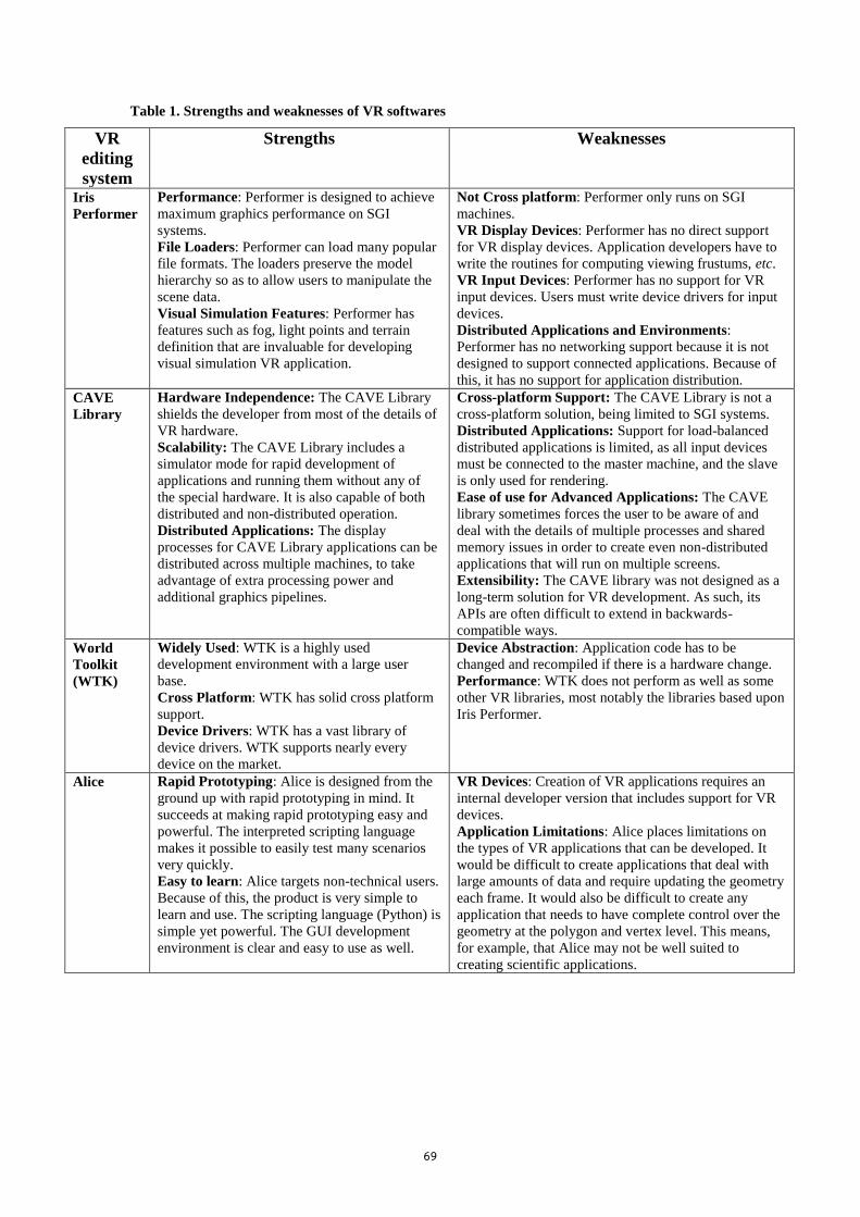
69
Table 1. Strengths and weaknesses of VR softwares
VR
editing
system
Strengths Weaknesses
Iris
Performer
Performance: Performer is designed to achieve
maximum graphics performance on SGI
systems.
File Loaders: Performer can load many popular
file formats. The loaders preserve the model
hierarchy so as to allow users to manipulate the
scene data.
Visual Simulation Features: Performer has
features such as fog, light points and terrain
definition that are invaluable for developing
visual simulation VR application.
Not Cross platform: Performer only runs on SGI
machines.
VR Display Devices: Performer has no direct support
for VR display devices. Application developers have to
write the routines for computing viewing frustums, etc.
VR Input Devices: Performer has no support for VR
input devices. Users must write device drivers for input
devices.
Distributed Applications and Environments:
Performer has no networking support because it is not
designed to support connected applications. Because of
this, it has no support for application distribution.
CAVE
Library
Hardware Independence: The CAVE Library
shields the developer from most of the details of
VR hardware.
Scalability: The CAVE Library includes a
simulator mode for rapid development of
applications and running them without any of
the special hardware. It is also capable of both
distributed and non-distributed operation.
Distributed Applications: The display
processes for CAVE Library applications can be
distributed across multiple machines, to take
advantage of extra processing power and
additional graphics pipelines.
Cross-platform Support: The CAVE Library is not a
cross-platform solution, being limited to SGI systems.
Distributed Applications: Support for load-balanced
distributed applications is limited, as all input devices
must be connected to the master machine, and the slave
is only used for rendering.
Ease of use for Advanced Applications: The CAVE
library sometimes forces the user to be aware of and
deal with the details of multiple processes and shared
memory issues in order to create even non-distributed
applications that will run on multiple screens.
Extensibility: The CAVE library was not designed as a
long-term solution for VR development. As such, its
APIs are often difficult to extend in backwards-
compatible ways.
World
Toolkit
(WTK)
Widely Used: WTK is a highly used
development environment with a large user
base.
Cross Platform: WTK has solid cross platform
support.
Device Drivers: WTK has a vast library of
device drivers. WTK supports nearly every
device on the market.
Device Abstraction: Application code has to be
changed and recompiled if there is a hardware change.
Performance: WTK does not perform as well as some
other VR libraries, most notably the libraries based upon
Iris Performer.
Alice Rapid Prototyping: Alice is designed from the
ground up with rapid prototyping in mind. It
succeeds at making rapid prototyping easy and
powerful. The interpreted scripting language
makes it possible to easily test many scenarios
very quickly.
Easy to learn: Alice targets non-technical users.
Because of this, the product is very simple to
learn and use. The scripting language (Python) is
simple yet powerful. The GUI development
environment is clear and easy to use as well.
VR Devices: Creation of VR applications requires an
internal developer version that includes support for VR
devices.
Application Limitations: Alice places limitations on
the types of VR applications that can be developed. It
would be difficult to create applications that deal with
large amounts of data and require updating the geometry
each frame. It would also be difficult to create any
application that needs to have complete control over the
geometry at the polygon and vertex level. This means,
for example, that Alice may not be well suited to
creating scientific applications.

71
Appendix V: Robot learning
Conventional vision-based methods for grasping objects typically require quantitatively correct
models of the robot’s own characteristics and of the relevant parts of the environments. Generating those
models and maintaining their accuracy in a changing and unpredictable world is difficult and expensive.
Object grasping independent of either the robot’s inbuilt quantitative models or pre-defined numerical
values of any parameter does not need any explicit calibration and, therefore, promises robustness. A
variety of methods have in recent years been developed for this challenging and difficult task. For
example, Cipolla and Hollinghurst, 1997, avoid using an exact kinematic model of the manipulator and
knowledge of the camera parameters by performing self-calibration at four known points, combined
with the use of visual feedback. Graefe, 1995, and Nguyen, 1997 avoid the necessity of calibration for
robots by a direct transition from visual input information to robot control commands. There has also
been work done in the area of eliminating the need for calibration of robots, such as the calibration of
the vision system. There is much work being done to increase the adaptability and flexibility of robots,
such as making them independent of world coordinates or making them able to automatically adapt to
various changing parameters. Algorithms have also been designed which allow robots to automatically
begin learning the environment, allowing them to recognize typical situations that they might be in
[Aycard and Washington, 2000].
A tool developed in the “LEGO” laboratory of Aarhus University, Denmark, called “Toybots”
[Lund and Pagliarini, 2000] allows users to play with evolutionary robotics tool for supporting the
evolution of populations of robots (e.g., pets); the users can select the behaviors they like better while
the robots are acting in the real world. “Toybots” is basically an interface to a user-guided genetic
algorithm in which the user selection substitutes the classical formal fitness function. This approach
allows for personalized evolution according to the user’s tastes, and at the same time letting users learn
about evolution in an intuitive way. The principle of using minimal simulation coupled with
reinforcement learning-based re-training in the real world helps to bridge the gap between simulation
and reality [Cañamero et al., 1999]. Complex behavior is achieved using a behavior-based system,
where the users evolve both the basic behavior modules and the behavior arbitrators. These ideas have
been applied in the interactive “LEGO-Mindstorms” football, where children can select behavioral
sequences to configure their players, and in the adaptive “LEGO” pet robot [Lund and Pagliarini, 2000].
Scárdua et al., 2000, developed a team of agents capable of learning cooperative behavior solely
by observing the impact of their actions in the environment. To achieve this goal, they have developed
an agent capable of learning to choose its actions by observing environment rewards. Their first phase of
the development, described in this paper, intends to assess a neural network as an action evaluator in the
robotic soccer domain.

71
Bhanu et al., 2001, presents the design, implementation and testing of a real-time system using
computer vision and machine learning techniques to demonstrate learning behavior in a miniature
mobile robot. The miniature robot through environmental sensing learns to navigate a maze by the
optimum route. Several reinforcement learning based algorithms, such as Q-learning, Q(λ)-learning, fast
on-line Q(λ)-learning and DYNA structure, were considered.
Carreras et al., 2002, propose a Neural-Q_learning approach designed for on-line learning of
simple and reactive robot behaviors. In this approach, the Q_function is generalized by a multi-layer
neural network (NN) allowing the use of continuous states and actions. The algorithm uses a database of
the most recent learning samples to accelerate and guarantee the convergence. Each Neural-Q_learning
function represents an independent, reactive and adaptive behavior which maps sensorial states to robot
control actions. A group of these behaviors constitutes a reactive control scheme designed to fulfill
simple missions. The paper centers on the description of the Neural-Q_learning based behaviors
showing their performance with an underwater robot in a target following task. Real experiments
demonstrate the convergence and stability of the learning system, pointing out its suitability for on-line
robot learning.
Heisele et al., 2001, presented several methods for face recognition and evaluated them with
respect to robustness against pose changes. They located facial components, extracted them, and
combined them into a feature vector which was classified by support vector machines (SVMs). Kim and
Kim, 2002, used SVMs for face recognition in real-time. Since SVMs were originally developed for
two-class classification, their basic scheme is extended for multiple recognition by adopting one-per-
class decomposition. In order to make a final classification from one-per-class SVM outputs, a NN was
used as the arbitrator. A facial sex classification system using SVMs was developed by Moghaddam and
Yang, 2001. The classification was tested with various kernels in order to explore the space of models
and performance. A Gaussian radial basis function (RBF) was found to perform the best (in terms of
error rate), followed by a cubic polynomial kernel as second best. By using a low resolution of 21-by-12
faces, they achieved a reliable sex classification. Text categorization is the process of sorting text
documents into one or more predefined categories or classes of similar documents [Basu et al., 2003].
Basu et al., 2003, trained 600 random documents and compared SVMs to NN classification. They
discovered significant differences in the performance of the SVMs over the NN. They concluded that
SVMs is preferable and less complex.

72
Appendix VI: ART-1
General
The ART-1 basic architecture is shown in Figure 1.
Figure 1. ART-1 basic architecture
There are three groups of neurons: an input processing field (F1 layer), the cluster units (F2
layer), and a mechanism for control and reset. F1 layer can be considered to consist of two parts, the
input and the interface portions, F1(a) and F1(b). To control similarity of patterns placed on the same
cluster, there are two sets of connections, top-down and bottom-up, between each unit in F1(b) and each
cluster unit in F2. F1(b) combines input signals from F1(a) and F2 layer to measure similarity between
an input signal and the weight vector for the specific cluster unit. The F2 layer is a competitive layer: the
cluster unit with the largest activation becomes the candidate to learn the input pattern. This cluster unit
is allowed to learn the input pattern depends on how similar its top-down weight is to the input vector.
The reset unit makes the decision, and other supplemental units are also needed to control the processing
of information in the network.
General operational procedure of ART-1 is shown in Figure 2.
F2 Layer (Clustering Units)
F1(b) Layer (Interface)
F1(a) Layer (Input)
Reset
Control
Units
Bo
tto
m-U
p
Lin
ks
To
p-D
ow
n
Lin
ks
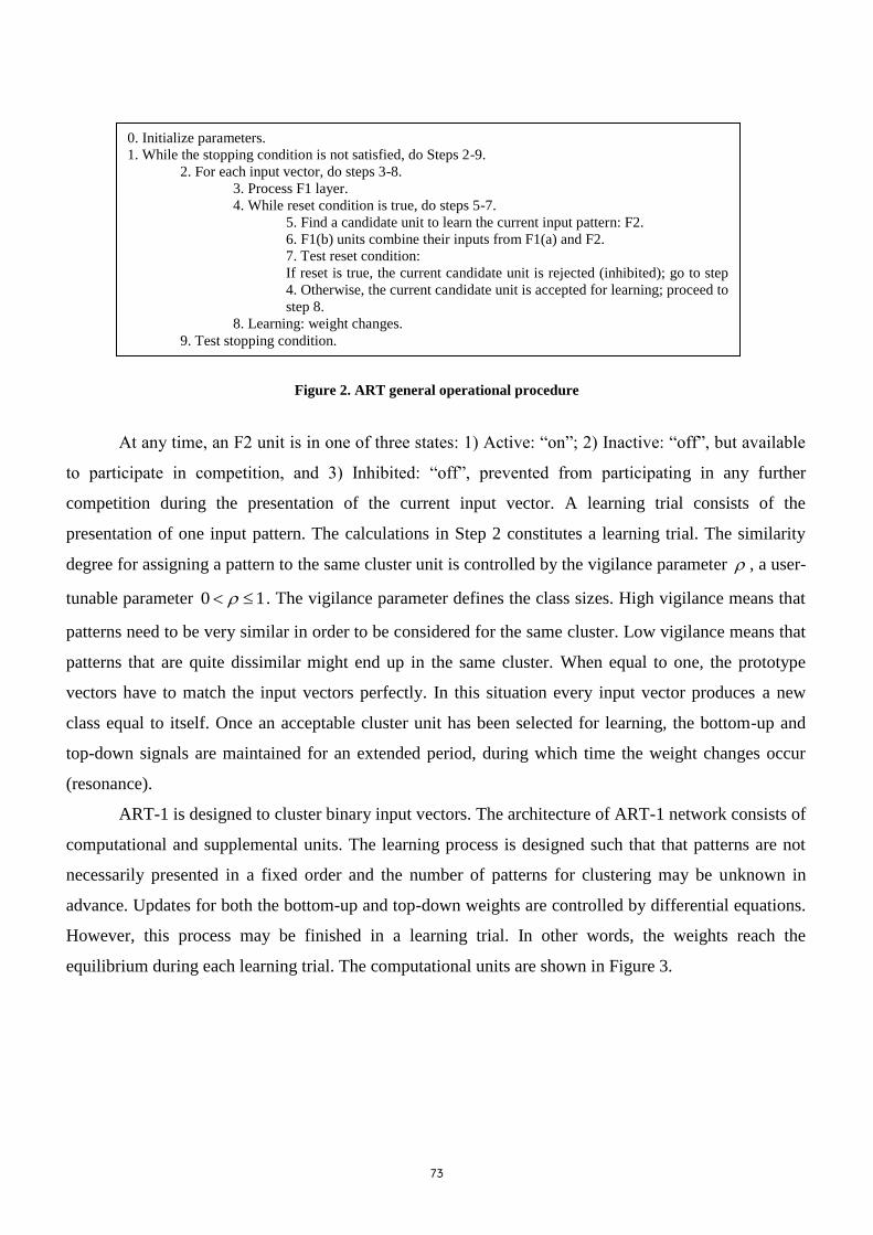
73
Figure 2. ART general operational procedure
At any time, an F2 unit is in one of three states: 1) Active: “on”; 2) Inactive: “off”, but available
to participate in competition, and 3) Inhibited: “off”, prevented from participating in any further
competition during the presentation of the current input vector. A learning trial consists of the
presentation of one input pattern. The calculations in Step 2 constitutes a learning trial. The similarity
degree for assigning a pattern to the same cluster unit is controlled by the vigilance parameter , a user-
tunable parameter 10 . The vigilance parameter defines the class sizes. High vigilance means that
patterns need to be very similar in order to be considered for the same cluster. Low vigilance means that
patterns that are quite dissimilar might end up in the same cluster. When equal to one, the prototype
vectors have to match the input vectors perfectly. In this situation every input vector produces a new
class equal to itself. Once an acceptable cluster unit has been selected for learning, the bottom-up and
top-down signals are maintained for an extended period, during which time the weight changes occur
(resonance).
ART-1 is designed to cluster binary input vectors. The architecture of ART-1 network consists of
computational and supplemental units. The learning process is designed such that that patterns are not
necessarily presented in a fixed order and the number of patterns for clustering may be unknown in
advance. Updates for both the bottom-up and top-down weights are controlled by differential equations.
However, this process may be finished in a learning trial. In other words, the weights reach the
equilibrium during each learning trial. The computational units are shown in Figure 3.
0. Initialize parameters.
1. While the stopping condition is not satisfied, do Steps 2-9.
2. For each input vector, do steps 3-8.
3. Process F1 layer.
4. While reset condition is true, do steps 5-7.
5. Find a candidate unit to learn the current input pattern: F2.
6. F1(b) units combine their inputs from F1(a) and F2.
7. Test reset condition:
If reset is true, the current candidate unit is rejected (inhibited); go to step
4. Otherwise, the current candidate unit is accepted for learning; proceed to
step 8.
8. Learning: weight changes.
9. Test stopping condition.
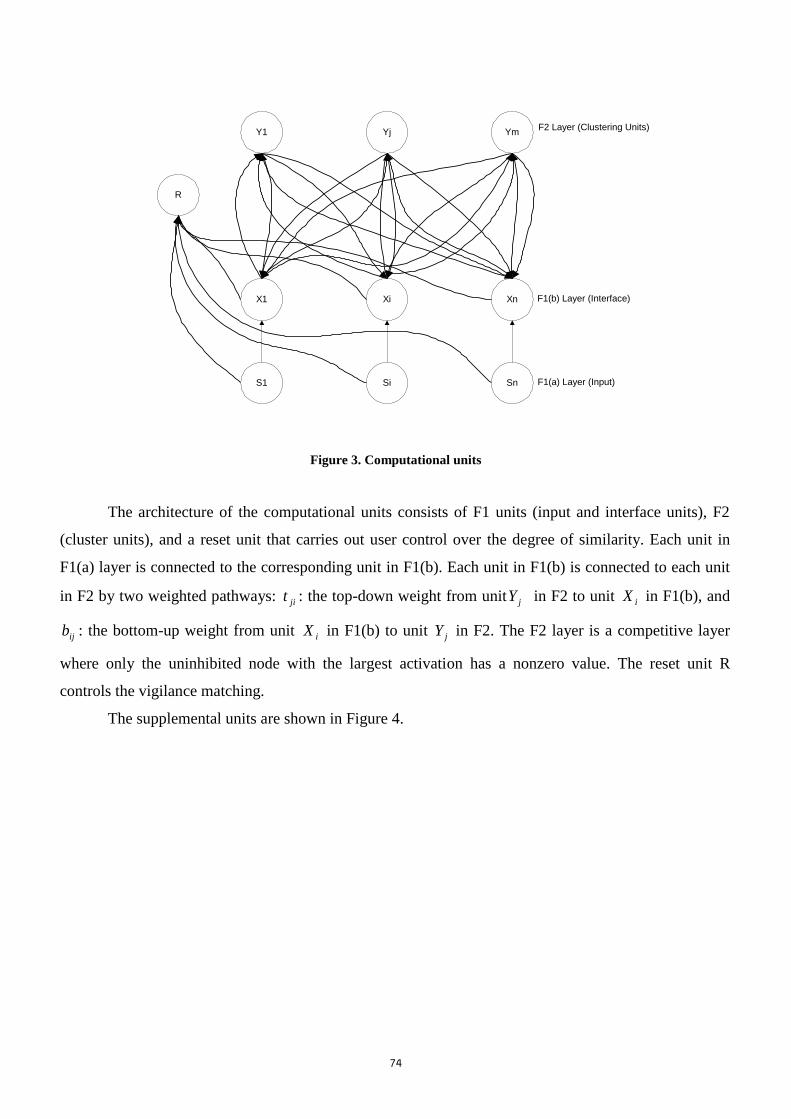
74
Figure 3. Computational units
The architecture of the computational units consists of F1 units (input and interface units), F2
(cluster units), and a reset unit that carries out user control over the degree of similarity. Each unit in
F1(a) layer is connected to the corresponding unit in F1(b). Each unit in F1(b) is connected to each unit
in F2 by two weighted pathways: jit : the top-down weight from unit jY in F2 to unit iX in F1(b), and
ijb : the bottom-up weight from unit iX in F1(b) to unit jY in F2. The F2 layer is a competitive layer
where only the uninhibited node with the largest activation has a nonzero value. The reset unit R
controls the vigilance matching.
The supplemental units are shown in Figure 4.
Y1 Yj Ym
X1 Xi Xn
S1 Si Sn
R
F2 Layer (Clustering Units)
F1(b) Layer (Interface)
F1(a) Layer (Input)
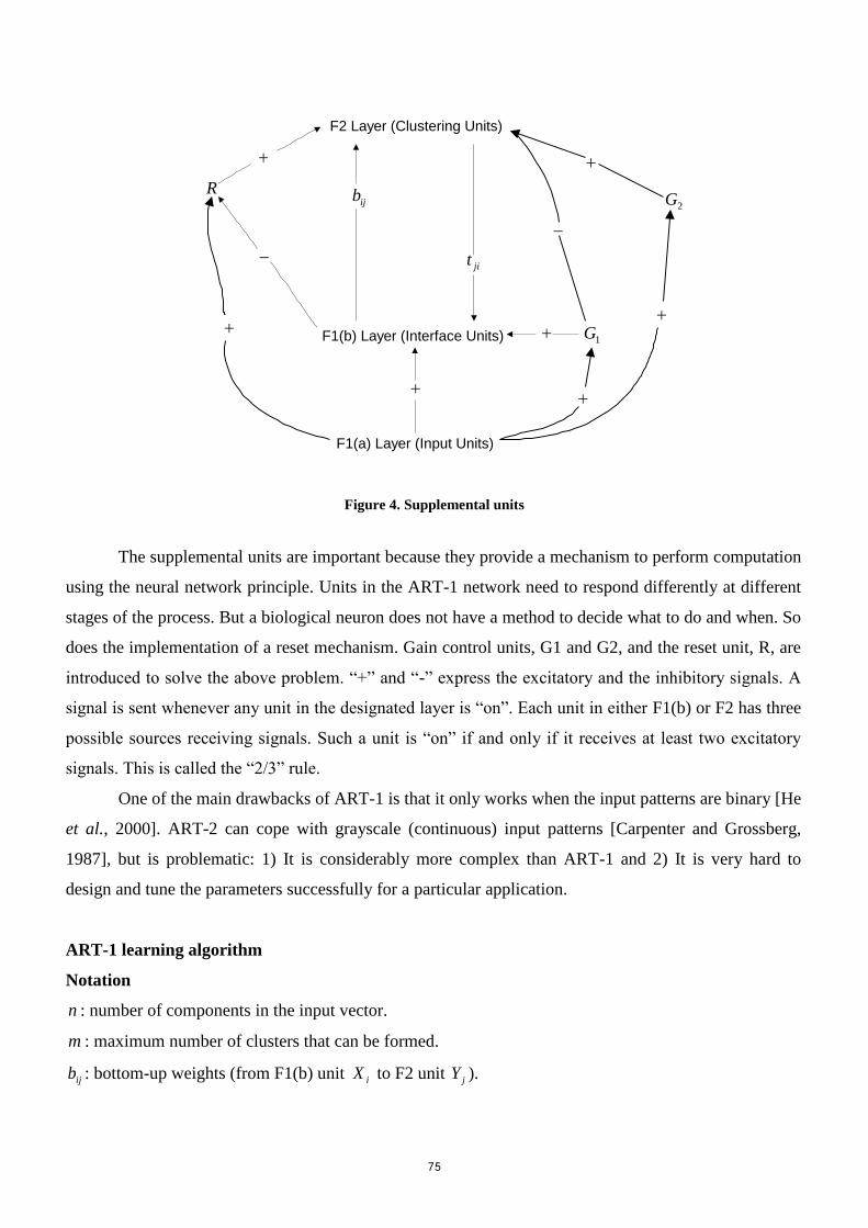
75
Figure 4. Supplemental units
The supplemental units are important because they provide a mechanism to perform computation
using the neural network principle. Units in the ART-1 network need to respond differently at different
stages of the process. But a biological neuron does not have a method to decide what to do and when. So
does the implementation of a reset mechanism. Gain control units, G1 and G2, and the reset unit, R, are
introduced to solve the above problem. “+” and “-” express the excitatory and the inhibitory signals. A
signal is sent whenever any unit in the designated layer is “on”. Each unit in either F1(b) or F2 has three
possible sources receiving signals. Such a unit is “on” if and only if it receives at least two excitatory
signals. This is called the “2/3” rule.
One of the main drawbacks of ART-1 is that it only works when the input patterns are binary [He
et al., 2000]. ART-2 can cope with grayscale (continuous) input patterns [Carpenter and Grossberg,
1987], but is problematic: 1) It is considerably more complex than ART-1 and 2) It is very hard to
design and tune the parameters successfully for a particular application.
ART-1 learning algorithm
Notation
n : number of components in the input vector.
m : maximum number of clusters that can be formed.
ijb : bottom-up weights (from F1(b) unit iX to F2 unit jY ).
F2 Layer (Clustering Units)
F1(b) Layer (Interface Units)
F1(a) Layer (Input Units)
ijb
jit
R
1G
2G
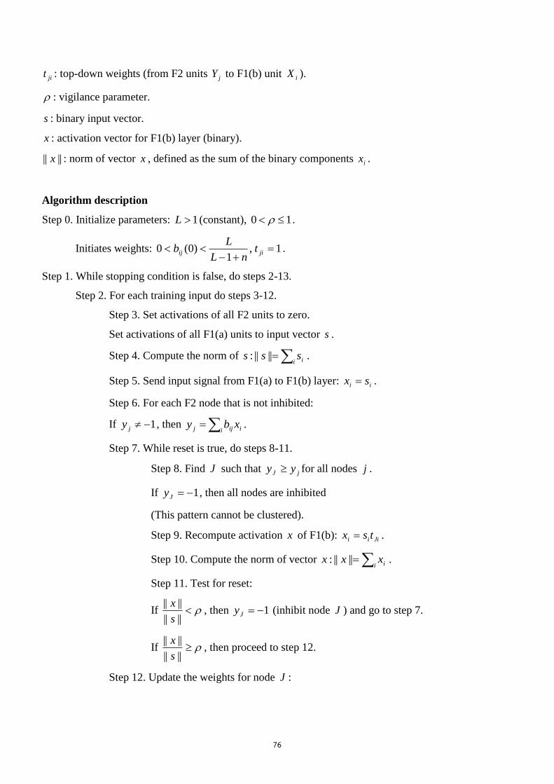
76
jit : top-down weights (from F2 units jY to F1(b) unit iX ).
: vigilance parameter.
s : binary input vector.
x : activation vector for F1(b) layer (binary).
|||| x : norm of vector x , defined as the sum of the binary components ix .
Algorithm description
Step 0. Initialize parameters: 1L (constant), 10 .
Initiates weights: 1,1
)0(0
jiij tnL
Lb .
Step 1. While stopping condition is false, do steps 2-13.
Step 2. For each training input do steps 3-12.
Step 3. Set activations of all F2 units to zero.
Set activations of all F1(a) units to input vector s .
Step 4. Compute the norm of i isss ||||: .
Step 5. Send input signal from F1(a) to F1(b) layer: ii sx .
Step 6. For each F2 node that is not inhibited:
If 1jy , then ii ijj xby .
Step 7. While reset is true, do steps 8-11.
Step 8. Find J such that jJ yy for all nodes j .
If 1Jy , then all nodes are inhibited
(This pattern cannot be clustered).
Step 9. Recompute activation x of F1(b): Jiii tsx .
Step 10. Compute the norm of vector i ixxx ||||: .
Step 11. Test for reset:
If ||||
||||
s
x, then 1Jy (inhibit node J ) and go to step 7.
If ||||
||||
s
x, then proceed to step 12.
Step 12. Update the weights for node J :
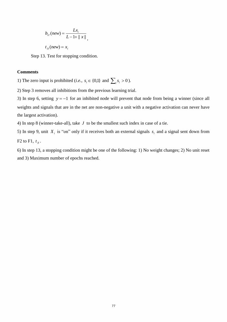
77
||||1)(
xL
Lxnewb i
iJ
,
iJi xnewt )(
Step 13. Test for stopping condition.
Comments
1) The zero input is prohibited (i.e., }1,0{is and 0i is ).
2) Step 3 removes all inhibitions from the previous learning trial.
3) In step 6, setting 1y for an inhibited node will prevent that node from being a winner (since all
weights and signals that are in the net are non-negative a unit with a negative activation can never have
the largest activation).
4) In step 8 (winner-take-all), take J to be the smallest such index in case of a tie.
5) In step 9, unit iX is “on” only if it receives both an external signals is and a signal sent down from
F2 to F1, Jit .
6) In step 13, a stopping condition might be one of the following: 1) No weight changes; 2) No unit reset
and 3) Maximum number of epochs reached.
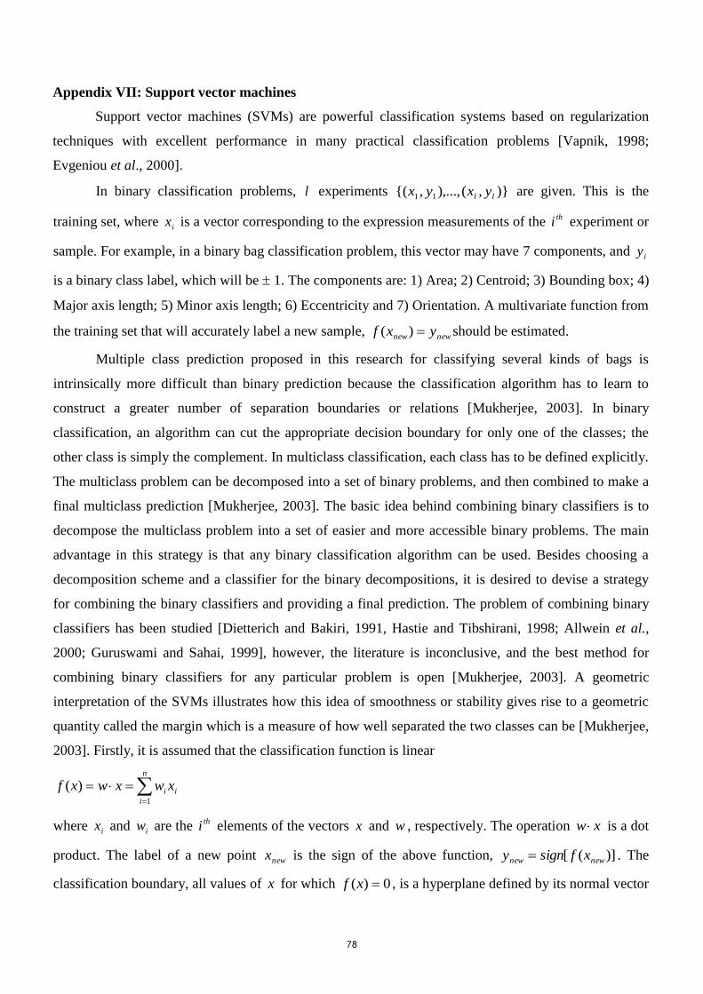
78
Appendix VII: Support vector machines
Support vector machines (SVMs) are powerful classification systems based on regularization
techniques with excellent performance in many practical classification problems [Vapnik, 1998;
Evgeniou et al., 2000].
In binary classification problems, l experiments )},(),...,,{( 11 ll yxyx are given. This is the
training set, where ix is a vector corresponding to the expression measurements of the thi experiment or
sample. For example, in a binary bag classification problem, this vector may have 7 components, and iy
is a binary class label, which will be 1. The components are: 1) Area; 2) Centroid; 3) Bounding box; 4)
Major axis length; 5) Minor axis length; 6) Eccentricity and 7) Orientation. A multivariate function from
the training set that will accurately label a new sample, newnew yxf )( should be estimated.
Multiple class prediction proposed in this research for classifying several kinds of bags is
intrinsically more difficult than binary prediction because the classification algorithm has to learn to
construct a greater number of separation boundaries or relations [Mukherjee, 2003]. In binary
classification, an algorithm can cut the appropriate decision boundary for only one of the classes; the
other class is simply the complement. In multiclass classification, each class has to be defined explicitly.
The multiclass problem can be decomposed into a set of binary problems, and then combined to make a
final multiclass prediction [Mukherjee, 2003]. The basic idea behind combining binary classifiers is to
decompose the multiclass problem into a set of easier and more accessible binary problems. The main
advantage in this strategy is that any binary classification algorithm can be used. Besides choosing a
decomposition scheme and a classifier for the binary decompositions, it is desired to devise a strategy
for combining the binary classifiers and providing a final prediction. The problem of combining binary
classifiers has been studied [Dietterich and Bakiri, 1991, Hastie and Tibshirani, 1998; Allwein et al.,
2000; Guruswami and Sahai, 1999], however, the literature is inconclusive, and the best method for
combining binary classifiers for any particular problem is open [Mukherjee, 2003]. A geometric
interpretation of the SVMs illustrates how this idea of smoothness or stability gives rise to a geometric
quantity called the margin which is a measure of how well separated the two classes can be [Mukherjee,
2003]. Firstly, it is assumed that the classification function is linear
i
n
i
i xwxwxf
1
)(
where ix and iw are the thi elements of the vectors x and w , respectively. The operation xw is a dot
product. The label of a new point newx is the sign of the above function, )]([ newnew xfsigny . The
classification boundary, all values of x for which 0)( xf , is a hyperplane defined by its normal vector
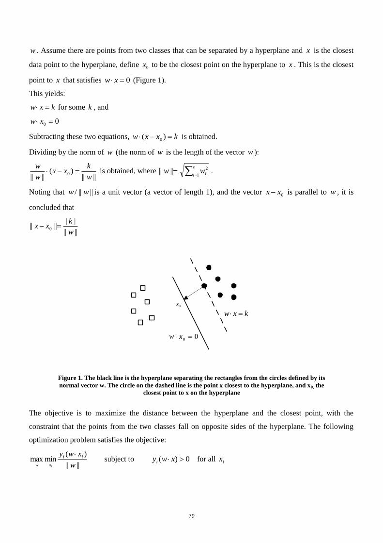
79
w . Assume there are points from two classes that can be separated by a hyperplane and x is the closest
data point to the hyperplane, define 0x to be the closest point on the hyperplane to x . This is the closest
point to x that satisfies 0 xw (Figure 1).
This yields:
kxw for some k , and
00 xw
Subtracting these two equations, kxxw )( 0 is obtained.
Dividing by the norm of w (the norm of w is the length of the vector w ):
||||)(
||||0
w
kxx
w
w is obtained, where
n
i iww1
2|||| .
Noting that ||||/ ww is a unit vector (a vector of length 1), and the vector 0xx is parallel to w , it is
concluded that
||||
|||||| 0
w
kxx
Figure 1. The black line is the hyperplane separating the rectangles from the circles defined by its
normal vector w. The circle on the dashed line is the point x closest to the hyperplane, and x0, the
closest point to x on the hyperplane
The objective is to maximize the distance between the hyperplane and the closest point, with the
constraint that the points from the two classes fall on opposite sides of the hyperplane. The following
optimization problem satisfies the objective:
||||
)(minmax
w
xwy ii
xw i
subject to 0)( xwyi for all ix
kxw
00 xw
0x

81
Note that ||)( kxwy when the point x is the circle closest to the hyperplane in Figure 1. It is required
that for the point ix closest to the hyperplane, 1k . This fixes a scale and unit to the problem and
results in a guarantee that 1)( ii wxy for all ix . All other points are measured with respect to the
closest point, which is distance 1 from the optimal hyperplane. Therefore, equivalently the problem to be
solved is:
||||
)(minmax
w
xwy ii
xw i
subject to 1)( ii xwy
An equivalent, but simpler problem [Vapnik, 1998] is
2||||2
1min w
w subject to 1)( ii xwy
Note that so far, only hyperplanes that pass through the origin were considered. In many
applications, this restriction is unnecessary, and the standard separable (i.e., the hyperplane can separate
the two classes) SVM problem is written as:
2
,||||
2
1min w
bw subject to 1)( bxwy ii
where b is a free threshold parameter that translates the optimal hyperplane relative to the origin. The
distance from the hyperplane to the closest points of the two classes is called the margin and is 2||||/1 w .
SVMs find the hyperplane that maximizes the margin. Figure 2 illustrates the advantage of a large
margin.
(a) (b)
Figure 2. (a) The maximum margin hyperplane separating two classes. The solid black line is the
hyperplane (wx + b = 0). The two dashed lines are those for the points in the two classes closest
to the hyperplane (wx + b = 1). A new point, the blank rectangle, is classified correctly in (a).
Note, the larger the margin the greater the deviation allowed or margin for error. (b) A non-
maximum margin hyperplane separating the two classes. Note, that the same new point is now
classified incorrectly. There is less margin for error.
1 bxw
1 bxw0 bxw
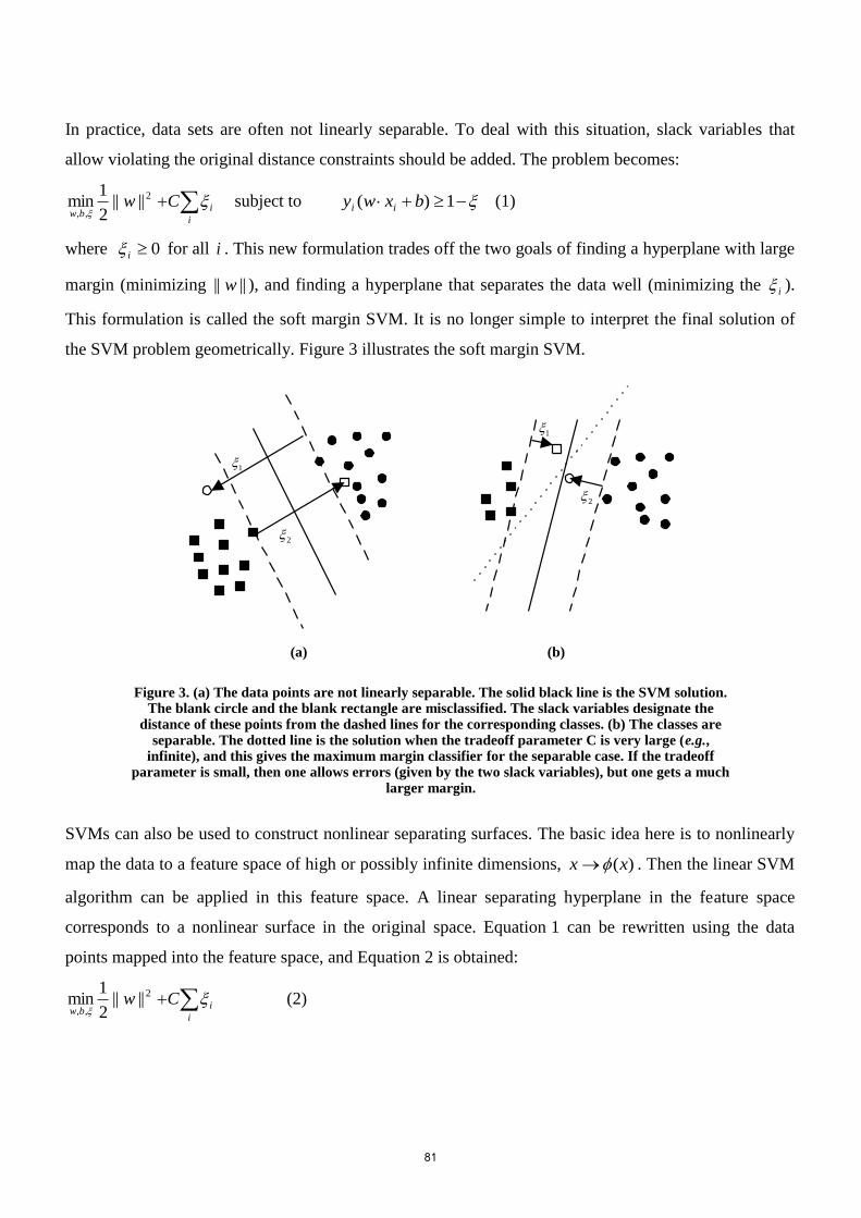
81
In practice, data sets are often not linearly separable. To deal with this situation, slack variables that
allow violating the original distance constraints should be added. The problem becomes:
i
ibw
Cw
2
,,||||
2
1min subject to 1)( bxwy ii (1)
where 0i for all i . This new formulation trades off the two goals of finding a hyperplane with large
margin (minimizing |||| w ), and finding a hyperplane that separates the data well (minimizing the i ).
This formulation is called the soft margin SVM. It is no longer simple to interpret the final solution of
the SVM problem geometrically. Figure 3 illustrates the soft margin SVM.
(a) (b)
Figure 3. (a) The data points are not linearly separable. The solid black line is the SVM solution.
The blank circle and the blank rectangle are misclassified. The slack variables designate the distance of these points from the dashed lines for the corresponding classes. (b) The classes are
separable. The dotted line is the solution when the tradeoff parameter C is very large (e.g., infinite), and this gives the maximum margin classifier for the separable case. If the tradeoff
parameter is small, then one allows errors (given by the two slack variables), but one gets a much larger margin.
SVMs can also be used to construct nonlinear separating surfaces. The basic idea here is to nonlinearly
map the data to a feature space of high or possibly infinite dimensions, )(xx . Then the linear SVM
algorithm can be applied in this feature space. A linear separating hyperplane in the feature space
corresponds to a nonlinear surface in the original space. Equation 1 can be rewritten using the data
points mapped into the feature space, and Equation 2 is obtained:
i
ibw
Cw
2
,,||||
2
1min (2)
1
2
1
2

82
0i for all i , where the vector w has the same dimensionality as the feature space and can be
thought of as the normal of a hyperplane in the feature space. The solution to the above optimization
problem has the form:
bxxcbxwxf i
l
i
i
)()()()(1
(3)
since the normal to the hyperplane can be written as a linear combination of the training points in the
feature space,
)(1
i
l
i
i xcw
.
For both the optimization problems (Equation 2) and the solution (Equation 3), the dot product of two
points in the feature spaces needs to be computed. This dot product can be computed without explicitly
mapping the points into feature space by a kernel function, which can be defined as the dot product for
two points in the feature space:
)()(),( jiji xxxxK (4)
The solution to the optimization problem now has the form:
bxxKcxf ji
l
i
i
),()(1
(5)
Most of the coefficients ic will be zero; only the coefficients of the points closest to the maximum
margin hyperplane in the feature space will have nonzero coefficients. These points are the support
vectors. Figure 4 illustrates a nonlinear decision boundary and the idea of support vectors.
Figure 4. The curve is the nonlinear decision boundary given by the SVM. The blank circles and
the blank rectangles are the support vectors. Only these points contribute in defining the
nonlinear decision boundary.

83
The following example illustrates the connection between the mapping into a feature space and the
kernel function. Assume that the area measured in pixels for two bags is, )(BAreaBriefcaseA and
)(SAeaSuitcaseAr . For each sample, there is an area vector x = (xBA, xSA). The following mapping
)(x is used:
}1,,,2,,{: 22
SABASABASABA xxxxxxx
If there are two samples x and z , then:
1
22
)1()()(),(
2222
2
SASABABA
SABASABASASABABA
zxzx
zzxxzxzx
zxzxzxK
is obtained, which is called a second order polynomial kernel. Note, that this kernel uses information
about both areas of individual bags and also areas of pairs of bags. The following two kernels, the
polynomial and Gaussian kernel, are commonly used:
pzxzxK )1(),( and )2/||||exp(),( 2zxzxK
Combining binary classifiers
Modern approaches for combining binary classifiers can be stated in terms of what is called
output coding [Dietterich and Bakiri, 1991, Hastie and Tibshirani, 1998; Allwein et al., 2000;
Guruswami and Sahai, 1999]. The basic idea behind output coding is the following: given k classifiers
trained on various partitions of the bag classes, a new example is mapped into an output vector. Each
element in the output vector is the output from one of the k classifiers, and a codebook is then used to
map from this vector to the class label. For example, given three classes, the first classifier may be
trained to discriminate classes 1 and 2 from 3, the second classifier is trained to discriminate classes 2
and 3 from 1, and the third classifier is trained to discriminate classes 1 and 3 from 2. A common output
coding that was proved to be accurate [e.g., Rifkin et al., 2002], the one-versus-all (OVA) [Mukherjee,
2003] will be used. In the OVA approach, given k bag classes, k independent classifiers are
constructed where the thi classifier is trained to separate samples belonging to class i from all others.
The codebook is a diagonal matrix, and the final prediction is based on the classifier that
produces the largest confidence (margin) [Rifkin et al., 2002]:
iki
fclass..1
maxarg
where if is the signed confidence measure of the thi classifier. Leave-one-out cross validation and an
independent test might be used to test the methodology. The confidence of the final call is the margin of
the winning SVM. When the largest confidence is positive the final prediction is considered a “high

84
confidence” call. If negative it is a “low confidence” call that can also be considered a candidate for a
no-call because no single SVM claims the sample as belonging to its recognizable class. Accuracy error
rates will be analyzed in terms of totals and also in terms of high and low confidence calls.

85
Appendix VIII: Reinforcement learning
Algorithms
Of the many reinforcement learning (RL) algorithms, perhaps the most widely used are Q-
learning [Watkins, 1989; Watkins and Dayan, 1992] and Sarsa [Rummery and Niranjan, 1994; Sutton,
1996]. Suppose the system observes a current state s , executes action a , receives immediate reward r ,
and then observes a next state 's . The Q-learning algorithm updates the current estimate, ),( asQk , of
),(* asQ using the following equation:
)1()],(max[),()1(),( ''
1'
'asQrasQasQ k
Aakkkk
s
,
where k is a time-varying learning-rate parameter. The values of all the other state-action pairs remain
unchanged in this update. If in the limit the action-values of all admissible state-action pairs are updated
infinitely often, and k decays with increasing k while obeying the usual stochastic approximation
conditions, then }{ kQ converges to *Q with probability of 1 [Jaakkola, 1994; Bertsekas and Tsitsiklis,
1996].
Sarsa is similar to Q-learning except that the maximum action-value for the next state on the
right-hand side of (1) is replaced by the action-value of the actual next state-action pair [Sutton, 1996]:
)2()],([),()1(),( ''
1 asQrasQasQ kkkkk ,
where 'a is the action executed in state 's . This algorithm is called Sarsa due to its dependence on s ,
a , r , 's , and 'a .
In particular, an estimate for ),(* asQ is obtained by combining the immediate reward r with a utility
estimate for the next state, )],([max)( '''' asQsU
Aa . The sum
),3()( 'sUr
called a 1-step corrected estimator, is an unbiased estimator for ),(* asQ when *QQ , since, by
definition
),4())],((),([),( ** asTVasREasQ
where ),(max)( ** asQsV Aa . The 1-step estimate is combined with the old estimate for ),( asQ using
a weighted sum:
),5()]([),()1(),( '
1 sUrasQasQ kkkk
where k is the learning rate. Finally, the system's control policy is updated using Equation 10
described later, and the cycle repeats.

86
Modeling robot-environment interaction
It is assumed that the robot-environment interaction can be modeled as a Markov Decision
Process (MDP). In MDP, the robot and the environment are modeled by two synchronized finite state
automatons interacting in a discrete time cyclical process model (Figure 1).
Figure 1. Basic model of robot-environment
Let S denote the set of possible environmental states, and A denotes the set of possible actions.
It is assumed that both S and A are discrete and finite. The dynamics of state transitions are modeled by
a transition function, T , which maps state-action pairs into next states ( SAxST : ). In general, the
transition may be probabilistic. If ts denotes the state at time t , and 1tS be the random variable
denoting the state at time 1t , then ).,(1 ttt asTS T is usually specified in terms of a set of transition
probabilities, )(',aP
ss, where )6()),(()( '
, ' sasTPaPss
.
Rewards generated by the environment are determined by a reward function, R , which maps
state into scalar rewards ( SR : ). The reward function is probabilistic and depends on the number
of items fell from a bag during lift and shaking operations. If tR be the random variable denoting the
reward received at time t , then )( tt aRR .
Notice that the system has a degree of control over the temporal evolution of the process since it
chooses an action at each time step. It is assumed that in selecting control actions the system's decision
is based solely upon the value of the current state. Under these circumstances the system behavior can be
specified by a control policy, which describes the action to execute given the current state. Formally, a
policy f is a function from states to actions ( ASf : ) where )(sf denotes the action to be
Agent
Environment
taaction
1tr
1ts
trreward
tsstate

87
performed in state s . The system's objective is to learn a control policy that maximizes some measure of
the total reward accumulated over time. In principle, any number of reward measures can be used,
however, the most prevalent measure is one based on a discounted sum of the reward received over
time. This sum is called the return and is defined for time t as
)7()(0 ntn
nrtreturn
where , called the temporal discount factor, is a constant between 0 and 1, and ntr is the reward
received at time nt . Because the process may be stochastic, the system's objective is to find a policy
that maximizes the expected return. For a fixed policy f , )(sV f is defined as the value function for f ,
to be the expected return, given that the process begins in state s and follows policy f thereafter. The
system's objective is to find a policy, *f , that for every state maximizes the value function. That is, find
*f , such that
)(max)(* sVsV fff
)8(Ss .
An important property of MDPs is that *f is well defined and guaranteed to exist. In particular,
the optimality theorem from dynamic programming [Bellman, 1957] guarantees that for a discrete time,
discrete state Markov decision problem there always exists a deterministic policy that is optimal.
Furthermore, a policy f is optimal if and only if it satisfies the relation
)),((max))(,( asQsfsQ fAa
f
)9(Ss
where ),( asQ f , called the action-value for state-action pair ),( as , is defined as the return the robot
expects to receive given that it starts in state s , applies action a next, and then follows policy f
thereafter [Bellman, 1957, Bertsekas, 1987]. Intuitively, a policy is optimal if and only if in each state,
s , the policy specifies the action that maximizes s 's action-value. That is,
af * such that )],([max),( '*
'* asQasQ
fAa
f
)10(Ss .
For a given MDP, the set of action-values for which Equation 9 holds is unique. These values are said to
define the optimal action-value function *Q for the MDP. If an MDP is completely specified a priori
(including the transition probabilities and reward distributions) then an optimal policy can be computed
directly using techniques from dynamic programming [Bellman, 1957, Ross, 1983, Bertsekas, 1987].
Because the interest here is robot learning, it is assumed that only the state space S and set of possible
actions A are known a priori and that the statistics governing T and R is unknown. Under these
circumstances the system cannot compute the optimal policy directly, but must explore its environment
and learn an optimal policy by trial and error.
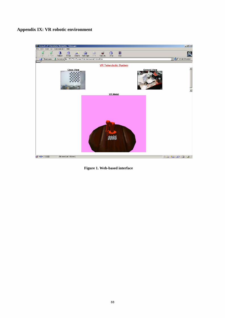
88
Appendix IX: VR robotic environment
Figure 1. Web-based interface

89
Figure 2. VR hierarchy

91
Appendix X: Operational control panels
Speed control
The “Speed” control panel (Figure 1) changes the speed of the real robot motion. The three
buttons “Velocity=20%”, “Velocity=50%” and “Velocity=100%” represent values of speeds correspond
to a percentage of the robot full speed which is 3.21 m/s according to the real “A255” robot
specifications [A255 Robot System, 1998]. When the system is powered-up, the speed setting is 50%.
Figure 1. Speed control panel
Grid control
The “3DGrid” control panel consists of an option button set (Figure 2). By choosing one at a
time of the options Layer0 to Layer8, a grid that contains 64 points appears in the virtual reality (VR)
model (Figure 3b-j). Each one of the associative points of layer1 to layer8 is located exactly 30cm in
“Alice” coordinates above the center of each one of the 64 checkerboard squares. Layer0 represents the
64 points that on the surface of the VR checkerboard. Clicking on a spatial point sends the VR robot
gripper over there. The “Hide All” option hides the layer points (Figure 3a). The “Show All” option
shows the entire layer points (Figure 3k). Figure 4 shows an example in which the robot gripper touches
the four extremist points of the highest layer (layer8).
Figure 2. 3DGrid control panel

91
(a) All the layers are hidden (b) Layer0 - checkerboard surface points
(c) Layer1 (d) Layer2
(e) Layer3 (f) Layer4
(g) Layer5 (h) Layer6
(i) Layer7 (j) Layer8

92
(k) All layers are shown
Figure 3. 3D layers
(a) Layer8 close right point (b) Layer8 close left point
(c) Layer8 far right point (d) Layer8 far left point
Figure 4. Layer8 extremist points
Views control
Using the “Views” control (Figure 5) enables the human operator (HO) to change the field-of-
view over the VR environment. There are three types of possible views: the close, the side and the front
(Figure 6).

93
Figure 5. Views control panel
(a) Close view
(b) Side view
(c) Front view
Figure 6. Three types of views
Shake control
By using the “Shake” control panel, the HO can choose two pairs of spatial points
(ShakePoint1, ShakePoint2, and ShakePoint3, ShakePoint4) for shaking a bag, and another point located
on the robot workspace for picking it up (PickUpPoint) (Figure 7). Clicking on the red cylinder, which is
located on the VR checkerboard and represents a bag (Figure 8) causes the VR robot to move there.
Clicking on the “PickUpPoint” button will send the location coordinates of the bag to the real robot
server that stores them. Choosing the four spatial points by using the “3Dgrid” control panel (example is

94
shown in Figure 9) and using the four buttons “ShakePoint1”, “ShakePoint2”, “ShakePoint3” and
“ShakePoint4” defines two pairs of points for shaking a bag. These four point coordinates are sent to the
robot server and stored there. The “Shake Batch” button causes the real robot to move toward the
location of the bag that was previously stored. Then it moves through each of the four points and their
coordinates are stored in the robot controller. After the points are stored in the robot controller, a
shaking action is performed in such a way that the robot moves from the first point to the second several
times and then from the third point to the forth additional several times (example is shown in Figures 10
and 11). If the HO desires performing more bag shaking, he may choose the buttons “ShakeMore-1-2”
that cause the robot to move for another cycle of shaking between the first and the second points, and
“ShakeMore-3-4” that does the same for the third and the forth points. The “ShakeMore-1-2-3-4” button
causes the robot to move between the track of all the four points several times. The “New Shake” button
resets the points and causes both the real and the VR robots to move toward their starting location
(Figure 12).
Figure 7. Shake control panel

95
Figure 8. Bag located on the VR checkerboard represented by a red cylinder
(a) First point of pair1 (b) Second point of pair1
(c) First point of pair2 (d) Second point of pair2
Figure 9. Spatial points example
Figure 10. Shaking action through two points
Point1 Point2
Point1 Point2
Point3
Point4
Red Cylinder

96
Figure 11. Shaking action through four points
Figure 12. Starting location of the VR robot
Off-line planning control
Path planning is performed through the “Off-line Planning Control Panel” (Figure 13). By
using the off-line control panel buttons, a HO can manipulate the VR robot arm location in positive or
negative X and Y increments. The value of an increment is constant and was chosen to be on the one
hand large enough for accomplishing a task in a reasonable time, and on the other hand not to be too
large, for allowing the VR robot to reach accurate positions in the VR scene. A value of 7.5mm (a
quarter of a checkerboard length) was determined to be reasonable. The buttons “X+” and “X-” move
the VR robot across the X axis direction, and the buttons “Y+” and “Y-” move it across the Y axis
direction. The gripper is assumed to be perpendicular to the workspace when moving the VR robot.
Other possibilities in the off-line control panel include the commands “Pick”, “Path Point” and
“Release”. When a HO wants to pick up an object, he has to manipulate the VR robot to be close enough
to it (1cm as “Alice” reports between the end of the gripper and the center of gravity of the object was
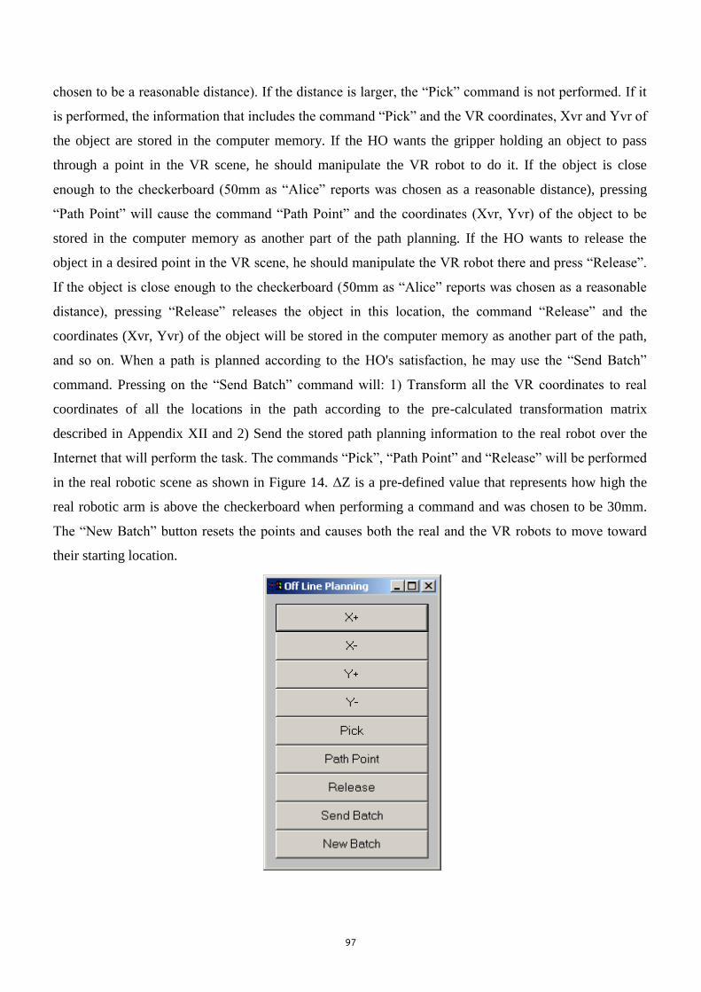
97
chosen to be a reasonable distance). If the distance is larger, the “Pick” command is not performed. If it
is performed, the information that includes the command “Pick” and the VR coordinates, Xvr and Yvr of
the object are stored in the computer memory. If the HO wants the gripper holding an object to pass
through a point in the VR scene, he should manipulate the VR robot to do it. If the object is close
enough to the checkerboard (50mm as “Alice” reports was chosen as a reasonable distance), pressing
“Path Point” will cause the command “Path Point” and the coordinates (Xvr, Yvr) of the object to be
stored in the computer memory as another part of the path planning. If the HO wants to release the
object in a desired point in the VR scene, he should manipulate the VR robot there and press “Release”.
If the object is close enough to the checkerboard (50mm as “Alice” reports was chosen as a reasonable
distance), pressing “Release” releases the object in this location, the command “Release” and the
coordinates (Xvr, Yvr) of the object will be stored in the computer memory as another part of the path,
and so on. When a path is planned according to the HO's satisfaction, he may use the “Send Batch”
command. Pressing on the “Send Batch” command will: 1) Transform all the VR coordinates to real
coordinates of all the locations in the path according to the pre-calculated transformation matrix
described in Appendix XII and 2) Send the stored path planning information to the real robot over the
Internet that will perform the task. The commands “Pick”, “Path Point” and “Release” will be performed
in the real robotic scene as shown in Figure 14. ΔZ is a pre-defined value that represents how high the
real robotic arm is above the checkerboard when performing a command and was chosen to be 30mm.
The “New Batch” button resets the points and causes both the real and the VR robots to move toward
their starting location.

98
Figure 13. Off-line control panel
(a) Pick (b) Path Point (c) Release
Figure 14. Path planning commands performed in the real robotic scene
Direct control
Direct control over both the VR and real robots is performed through the “Direct Control
Panel” that is shown in Figure 15. By using the “Direct Control Panel”, a HO can manipulate both the
VR and the real robots to move in the X, Y, and Z directions in real-time. It also allows opening and
closing the gripper. The increment of a movement is a pre-defined value and it was set to a reasonable
value of 7.5mm (a quarter of a checkerboard length). The “Starting Point” button sends both the VR and
real robots to their starting position.
Move to point (0, 0, +∆Z)
Move to point (∆X, ∆Y, 0)
Open Gripper
Move to point (0, 0, -∆Z(
Close Gripper
Move to point (0, 0, +∆Z)
Move to point (∆X, ∆Y,0)
Move to point (0, 0, -∆Z)
Move to point (0, 0, +∆Z)
Move to point ( ∆X, ∆Y, 0)
Move to point (0, 0, -∆Z)
Open Gripper

99
Figure 15. Direct control panel
High level to low level language control
By using the “High Level (HL) to Low Level (LL) Language” control panels exist in the VR
interface, a HO can plan complex robot trajectories. A trajectory consists of a combination of three HL
commands: pick an object, touch the object in a path point(s) located on the robotic platform and release
an object. The system is capable of using up to three plans that can be run independently. These plans
can be changed during system operation and in real-time, which gives the system the flexibility of
unlimited HL to LL number of plans. When a plan was designed by the HO through the HL to LL
control panel shown in Figure 16, he can send it as a batch to the real robot controller which transfers
the HL to LL commands, then the real robot performs the trajectory. Examples for HL to LL plans are
shown in Figures 17, 18 19 and 20.

111
Figure 16. High level to low level language control panel
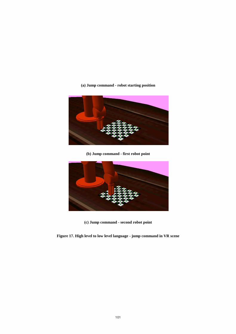
111
(a) Jump command - robot starting position
(b) Jump command - first robot point
(c) Jump command - second robot point
Figure 17. High level to low level language - jump command in VR scene
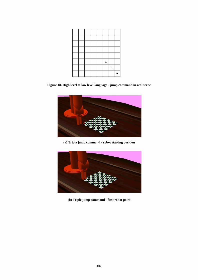
112
Figure 18. High level to low level language - jump command in real scene
(a) Triple jump command - robot starting position
(b) Triple jump command - first robot point

113
(c) Triple jump command - second robot point
(d) Triple jump command - third robot point
(e) Triple jump command - forth robot point
Figure 19. High level to low level language - triple jump command in VR scene

114
Figure 20. High level to low level language - triple jump command in real scene

115
Appendix XI: Kinematics
Top view over the robot arm is shown in Figure 1. “H” represents the sum of lengths of the
shoulder and the elbow. This distance is the length starting from the robot base-point ( BP ( to the gripper
end point ( 2P ).
Figure 1. Top view over the robot arm
The x and the y values are the horizontal and vertical values of the robot gripper position related to the
robot base-point.
The trigonometric equation for B is:
x
yB arctan
The relationship between H, x and y is:
22 yxH
The side view of the VR robotic chain is shown in Figure 2. It is assumed that the gripper is always
perpendicular to the robot workspace.
B
H
X
Y
BP
2P
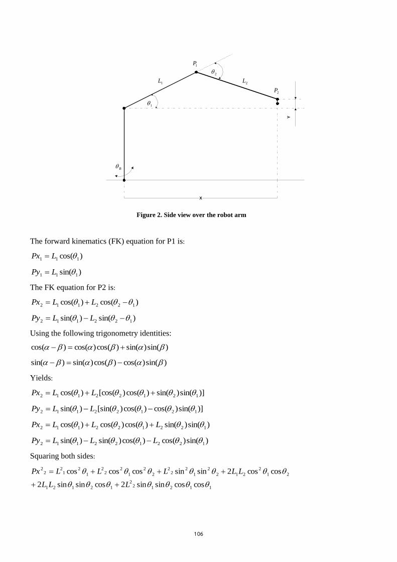
116
Figure 2. Side view over the robot arm
The forward kinematics (FK) equation for P1 is:
)cos( 111 LPx
)sin( 111 LPy
The FK equation for P2 is:
)cos()cos( 122112 LLPx
)sin()sin( 122112 LLPy
Using the following trigonometry identities:
)sin()sin()cos()cos()cos(
)sin()cos()cos()sin()sin(
Yields:
)]sin()sin()cos()[cos()cos( 12122112 LLPx
)]sin()cos()cos()[sin()sin( 12122112 LLPy
)sin()sin()cos()cos()cos( 122122112 LLLPx
)sin()cos()cos()sin()sin( 122122112 LLLPy
Squaring both sides:
112122
12121
21
2
212
2
1
22
2
2
2
1
22
2
1
21
22
2
coscossinsin2cossinsin2
coscos2sinsincoscoscos
LLL
LLLLLPx
1
2
1L 2L
B
1P
2P
X
Y

117
212122
21
2
21
211212
2
1
22
2
2
2
1
22
2
1
21
22
2
coscossinsin2cossin2
sincossin2cossinsincossin
LLL
LLLLLPy
Re-arranging:
)sin(coscos2)sin(cossin
)sin(coscos)sin(cos
1
2
1
2
2211
2
1
2
2
22
2
1
2
1
2
2
22
2
1
2
1
21
22
22
2
LLL
LLPyPx
22122
12
22
22 cos2 LLLLPyPx
21
22
22
22
12
22
cosLL
PyPxLL
21
22
22
22
12
22
arccosLL
PyPxLL
Solving 1 :
Figure 3. Side view over the robot arm
xy /)tan( 3
)cos(
)sin()tan(
221
224
LL
L
431
Using the identity )tan()tan(1
)tan()tan()tan(
and doing some substitution yields:
)tan()tan( 431
1
2
1L 2L
B
1P
2P
X
Y
3
4

118
x
y
x
y
sin
cosarctan3
)cos(
)sin(arctan
221
224
LL
L
)cos(
)sin(1
)cos(
)sin(
)tan(
221
22
221
22
1
LL
L
x
y
LL
L
x
y
Multiplying by x yields:
)cos(
)sin(
)cos(
)sin(
)tan(
221
22
221
22
1
LL
yLx
LL
xLy
)sin())cos((
)sin())cos(()tan(
22221
222211
yLLLx
xLLLy
)sin())cos((
)sin())cos((arctan
22221
222211
yLLLx
xLLLy
Now, given any position (x, y and z), the angles required to reach it are calculated.

119
Appendix XII: Transformation matrix
Table 1. Intersection coordinates
Point Num. VR Robot Coordinate (cm) Real Robot Coordinates (cm)
- Xvr* Yvr* Xr** Yr** 0 -21.15 18.16 26.5 -24
1 -21.15 13.62 26.5 -18
2 -21.15 9.08 26.5 -12
3 -21.15 4.54 26.5 -6
5 -21.15 -4.54 26.5 6
6 -21.15 -9.08 26.5 12
7 -21.15 -13.62 26.5 18
8 -21.15 -18.16 26.5 24
9 -25.69 18.16 32.5 -24
10 -25.69 13.62 32.5 -18
11 -25.69 9.08 32.5 -12
12 -25.69 4.54 32.5 -6
14 -25.69 -4.54 32.5 6
15 -25.69 -9.08 32.5 12
16 -25.69 -13.62 32.5 18
17 -25.69 -18.16 32.5 24
18 -30.23 18.16 38.5 -24
19 -30.23 13.62 38.5 -18
20 -30.23 9.08 38.5 -12
21 -30.23 4.54 38.5 -6
23 -30.23 -4.54 38.5 6
24 -30.23 -9.08 38.5 12
25 -30.23 -13.62 38.5 18
26 -30.23 -18.16 38.5 24
27 -34.77 18.16 44.5 -24
28 -34.77 13.62 44.5 -18
29 -34.77 9.08 44.5 -12
30 -34.77 4.54 44.5 -6
32 -34.77 -4.54 44.5 6
33 -34.77 -9.08 44.5 12
34 -34.77 -13.62 44.5 18
35 -34.77 -18.16 44.5 24
* vr - Virtual Reality
** r - Real

111
0 1 2 3 5 6 7 8
910 11 12 14 15 16
17
1819 20 21 23 24 25
26
2728 29 30 32 33 34
35
6 cm
6 cm
(Yr-) (Yr+)
Robot
26.5
cm
(Xr+)
(0,0)
(Xr-)
Figure 1. Intersection points taken from the real robotic environment for creating the
transformation matrix

111
0 1 2 3 5 6 7 8
910 11 12 14 15 16
17
1819 20 21 23 24 25
26
2728 29 30 32 33 34
35
4.5
4
cm
4.54
cm
(Yvr+) (Yvr-)
Robot
21.15
cm
(Xvr-)
(0,0)
(Xvr+)
Figure 2. Intersection points taken from the VR environment for creating the
transformation matrix
In the aligning a pair of shapes method, given two similar shapes, 1x (the virtual reality (VR)
environment) and 2x (the real environment), a rotation , a scale s ,and a translation ),( yx tt should be
chosen for mapping 2x onto )(xM so as to minimize the weighted sum:
))(())(( 2121 xMxWxMxE T
where:
yjkjk
xjkjk
jk
jk
tysxs
tysxs
y
xM
)cos()sin(
)sin()cos()(
and W is a diagonal matrix of weights for each point.
When cossax and sinsay then the least squares approach (differentiating with respect to each
of the variables xa ,ya ,xt ,yt ) leads to a set of four linear equations:
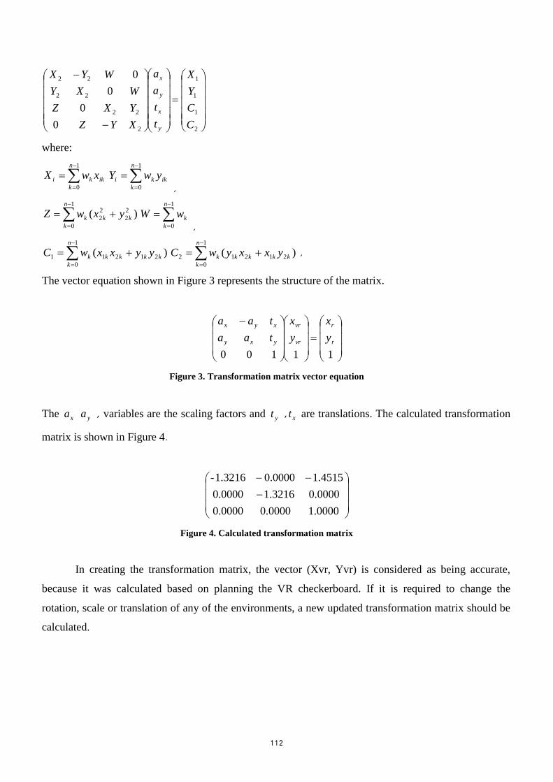
112
2
1
1
1
2
22
22
22
0
0
0
0
C
C
Y
X
t
t
a
a
XYZ
YXZ
WXY
WYX
y
x
y
x
where:
1
0
n
k
ikki xwX
,
1
0
n
k
ikki ywY
1
0
2
2
2
2 )(n
k
kkk yxwZ
,
1
0
n
k
kwW
1
0
21211 )(n
k
kkkkk yyxxwC ,
1
0
21212 )(n
k
kkkkk yxxywC
The vector equation shown in Figure 3 represents the structure of the matrix.
11100
r
r
vr
vr
yxy
xyx
y
x
y
x
taa
taa
Figure 3. Transformation matrix vector equation
The xa ,ya variables are the scaling factors and xt ,yt are translations. The calculated transformation
matrix is shown in Figure 4.
0000.10000.00000.0
0000.03216.10000.0
4515.10000.01.3216-
Figure 4. Calculated transformation matrix
In creating the transformation matrix, the vector (Xvr, Yvr) is considered as being accurate,
because it was calculated based on planning the VR checkerboard. If it is required to change the
rotation, scale or translation of any of the environments, a new updated transformation matrix should be
calculated.

113
Table 2. Intersection points and their corresponding parameters (cm)
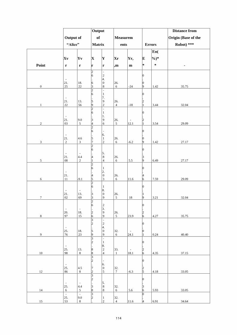
114
Output of
“Alice”
Output
of
Matrix
Measurem
ents Errors
Distance from
Origin (Base of the
Robot) ***
Point
Xv
r
Yv
r
X
r
Y
r
Xr
,m
Yr,
m
E
*
En(
%)*
* -
0
-
21.
25
18.
22
2
6.
6
3
-
24.
0
8
26.
6 -24
0.
0
9 1.42 35.75
1
-21.
22
13.
56
2
6
.5
9
-
1
7.9
2
26.
4 -18
0
.2
1 3.44 32.04
2
-
21.
03
9.0
5
2
6.
3
4
-
11.
9
6
26.
5
-
12.1
0.
2
1 3.54 29.09
3
-21.
2
4.6
3
2
6
.5
7
-
6.1
2
26.
6 -6.2
0
.0
9 1.42 27.17
5
-
21.08
-
4.42
26
.
41
5.
84
26.6 5.5
0
.
39 6.49 27.17
6
-21.
11 -9.1
2
6
.4
5
1
2.0
3
26.
6 11.6
0
.4
6 7.59 29.09
7
-
21.02
-
13.69
26
.
33
1
8.
09
26.5 18
0
.
19 3.21 32.04
8
-20.
97
-18.
15
2
6
.2
6
2
3.9
9
26.
5 23.9
0
.2
6 4.27 35.75
9
-
25.76
18.23
32
.
59
-2
4.
09
32.6
-24.1
0
.
01 0.24 40.40
10
-
25.
98
13.
8
3
2.
8
8
-
18.
2
4
33.
1
-
18.1
0.
2
6 4.35 37.15
12
-
25.86
4.58
32
.
72
-
6.
05
32.7 -6.3
0
.
25 4.18 33.05
14
-
25.
6
-
4.4
5
3
2.
3
8
5.
8
8
32.
6 5.6
0.
3
6 5.93 33.05
15
-25.
53
-9.0
8
32
.
1
2
32.
4 11.6
0.
4 6.91 34.64
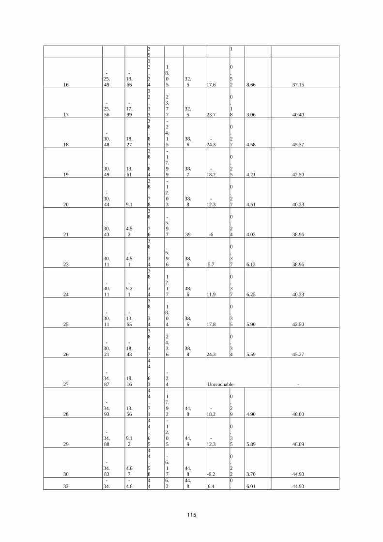
115
2
9
1
16
-
25.49
-
13.66
32
.
24
1
8.
05
32.5 17.6
0
.
52 8.66 37.15
17
-
25.
56
-
17.
99
3
2.
3
3
23.
7
7
32.
5 23.7
0.
1
8 3.06 40.40
18
-
30.48
18.27
38
.
83
-2
4.
15
38.6
-24.3
0
.
27 4.58 45.37
19
-
30.
49
13.
61
3
8.
8
4
-
17.
9
9
38.
7
-
18.2
0.
2
5 4.21 42.50
20
-
30.44 9.1
38
.
78
-1
2.
03
38.8
-12.3
0
.
27 4.51 40.33
21
-
30.
43
4.5
2
3
8.
7
6
-5.
9
7 39 -6
0.
2
4 4.03 38.96
23
-30.
11
-4.5
1
3
8
.3
4
5.9
6
38.
6 5.7
0
.3
7 6.13 38.96
24
-
30.
11
-
9.2
1
3
8.
3
4
12.
1
7
38.
6 11.9
0.
3
7 6.25 40.33
25
-30.
11
-13.
65
3
8
.3
4
1
8.0
4
38.
6 17.8
0
.3
5 5.90 42.50
26
-
30.
21
-
18.
43
3
8.
4
7
24.
3
6
38.
8 24.3
0.
3
4 5.59 45.37
27
-34.
87
18.
16
4
4
.6
3
-2
4 Unreachable -
28
-
34.93
13.56
44
.
71
-1
7.
92
44.8
-18.2
0
.
29 4.90 48.00
29
-34.
88
9.1
2
4
4
.6
5
-
1
2.0
5
44.
9
-
12.3
0
.3
5 5.89 46.09
30
-
34.83
4.67
4
4
.
58
-
6.
17
44.8 -6.2
0
.
22 3.70 44.90
32
-
34.
-
4.6
4
4
6.
2
44.
8 6.4
0
. 6.01 44.90
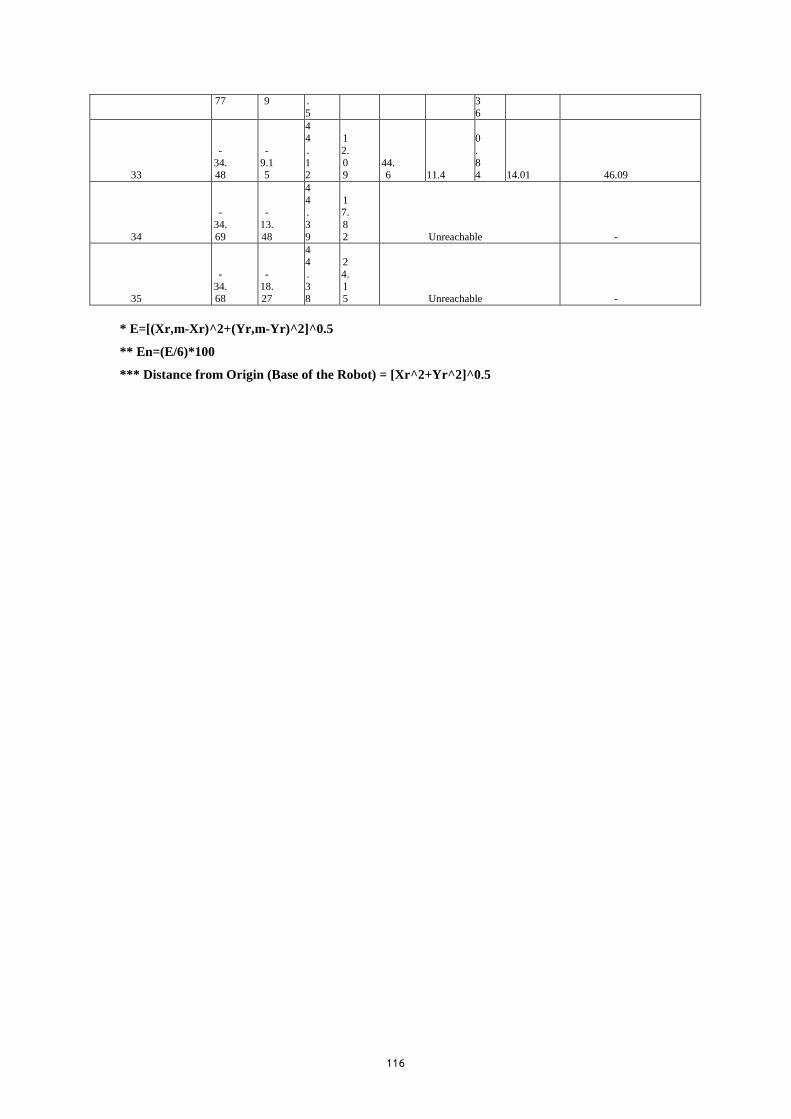
116
77 9 .
5
3
6
33
-
34.48
-
9.15
44
.
12
1
2.
09
44.6 11.4
0
.
84 14.01 46.09
34
-
34.
69
-
13.
48
4
4.
3
9
17.
8
2 Unreachable -
35
-
34.68
-
18.27
44
.
38
2
4.
15 Unreachable -
* E=[(Xr,m-Xr)^2+(Yr,m-Yr)^2]^0.5
** En=(E/6)*100
*** Distance from Origin (Base of the Robot) = [Xr^2+Yr^2]^0.5
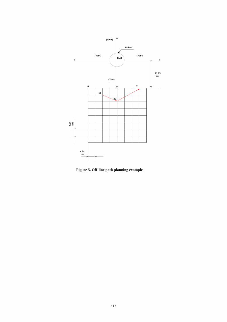
117
4.5
4
cm
4.54
cm
(Yvr+) (Yvr-)
Robot
21.15
cm
(Xvr-)
(0,0)
(Xvr+)
0
22
11
7
Figure 5. Off-line path planning example

118
Figure 6. Off-line path planning flow chart example
Start
Move VR Robot
Arm Manually
toward a Soldier
Located at Point
11
Is the VR Gripper
Close Enough to
the Soldier
Located at Point
11?
No Yes
Pick Up
Solider 11
Move VR Robot
Arm Manually
Toward Point 22
Is the VR Gripper
Close Enough to
Point 22?
NoYes
Move VR Robot
Arm Manually
Toward Point 7
Is the Gripper
Close Enough to
Point 7?
No Yes
Release the
Soldier at Point
7
End

119
Table 3. Path performing measurements

121
Point 11 (32.5, -
12.0) cm
Point 22 (38.5, 0)
cm
Point 7 (26.5, 18.0)
cm
Was the
Path
Perform
ed
Successf
ully?
Coordi
nates
(cm) Errors
Coordin
ates
(cm)
Err
ors
Coordin
ates
(cm) Errors
Experi
ment
Num. Yes/No
X
r
,
m
Y
r
,
m
E
*
E
n
*
X
r,
m
Y
r,
m
E
*
E
n
*
X
r
,
m
Y
r,
m
E
*
En
*
1 Yes
3
2
.6
-1
2
.3
0
.1
1
.
67
38.7
0.3
0
.
13
2
.
17
2
6
.7
18.1
0
.
05
0.83
2 Yes
32
.
4
-
12
.
3
0
.
1
1.
6
7
38
.7
0.
1
0.
0
5
0.
8
3
26
.
5
18.
3
0.
0
9
1.5
0
3 Yes
3
2.
7
-
1
2.
4
0.
2
3
.3
3
38
.5
-0.
2
0
.0
4
0
.6
7
2
6.
7
18.
4
0.
2
3.3
3
4 Yes
32
.
5
-
12
.
3
0.
0
9
1.
5
0
38
.3
0.
2
0.
0
8
1.
3
3
26
.
3
17.
8
0.
0
8
1.3
3
5 Yes
3
2.
6
-
1
2.
1
0
.0
2
0
.3
3
38
.7
0.
3
0
.1
3
2
.1
7
2
6.
5
17.
9
0
.0
1
0.1
7
6 Yes
32
.3
-
11
.8
0.
08
1.
33
38.8
0.3
0.
18
3.
00
26
.7
18.2
0.
08
1.33
7 Yes
3
2.
4
-
1
2.
0
0
.0
1
0
.1
7
38
.4
0.
2
0
.0
5
0
.8
3
2
6.
6
18.
3
0.
1
1.6
7
8 Yes
3
2
.5
-1
2
.1
0
.
01
0
.
17
38.5
0.1
0
.
01
0
.
17
2
6
.5
18.0 0
0.00
9 Yes
3
2.
7
-
1
2.
3
0
.1
3
2
.1
7
38
.7
0.
3
0
.1
3
2
.1
7
2
6.
8
18.
3
0
.1
8
3.0
0
10 Yes
3
2
.4
-1
2
.1
0
.
02
0
.
33
38.4
-
0.1
0
.
02
0
.
33
2
6
.4
18.0
0
.
01
0.17
* Xr,m & Yr,m - Manually Measured Coordinates

121
** E=[(Xr,m-Xr)^2+(Yr,m-Yr)^2]^0.5
*** En=(E/6)*100

122
6 cm
6 cm
(Yr-) (Yr+)
Robot
26.5
cm
(Xr+)
(0,0)
(Xr-)
0
16
Figure 7. Point 0 and point 16, used in the real environment for the repeatability test
Table 4. Repeatability test using point 0 and point 16

123
Point 0 Point 16
Measurement
Num. X (mm) Y (mm) X (mm) Y (mm)
Distance
Between
Point 0 to
Point 16
(mm) *
1 264.9951 -240.016 325.0674 180.0395 424.3296
2 264.9922 -240.028 325.0372 180.0228 424.3202
3 264.9999 -239.992 325.0429 179.9518 424.2149
4 264.9922 -240.028 325.0435 179.9151 424.2145
5 265.0132 -240.004 325.0686 179.966 424.2426
6 265.0208 -239.969 325.1305 180.0003 424.2495
7 264.9999 -239.992 324.9964 180.0002 424.2562
8 264.9999 -239.992 325.0429 179.9518 424.2149
9 265.0208 -239.969 325.064 179.9635 424.2037
10 265.0076 -239.957 325.0529 179.9944 424.2226
* Distance Between Point 0 to Point 16 = [(X61-X0)^2+(Y16-Y0)^2]^0.5