a hybrid g a to solve non-linear mixed integer programming

230

A Hybrid G A to Solve Non-linear Mixed Integer Programming Programs: An Efficient Method for Reliability System Design

Changyoon Lee* and Mitsuo Gen**

*SCM & Logistics Research Center Hanyang University

Ansan 426-791 , Korea E-mail: [email protected]

**Dept. of Industrial & Inform. Systems Engg. Ashikaga Institute of Technology

Ashikaga 326-8558, Japan E-mail: [email protected]

Abstract: In this paper, we discuss non-linear mixed integer programming (nMIP) models which should be simultaneously determined both continuous decision variables and discrete decision variables. This problem is more difficult to solve than the non-linear integer programming (niP) problem because of the exitance of several type of decision variable to represent the real world more actually. Recently, several researchers have obtained acceptable and satisfactory results by using genetic algorithms (GAs) for nMIP problems. When such problems become large, however, GA has a lot of enumeration of feasible solutions due to broad continuous search space. Recently, hybridized GA combined with a neural network technique (NN-hGA) is proposed to overcome this kind of difficulties. In order to more carefully search the near optimal region in GA procedure, we employ the simplex search method as a local search technique to deal with continuous decision variables. Numerical experiments and comparison with the previous works demonstrate the efficiency of our proposed method. Keywords: Non-linear mixed integer programming, Genetic algorithm, Neural network technique.

1 Introduction

In the past few decades, many researchers have proposed various methods for solving the non-linear integer programming (niP) problems aris-ing in engineering applications. While, many practical problems in process synthesis and pro-cess optimization lead to mathematical optimiza-tion models in continuous decision variables and discrete decision variables with nonlinear con-straints, i.e., the mathematical formulation of such a problem becomes a non-linear mixed in-teger programming (nMIP) problem. This nMIP problem is more difficult to solve than the niP problem because it should be simultaneously de-termined two types of decision variables.

An enormous increase in the capabilities for solving niP problems and nMIP problems has oc-curred [1, 2, 3]. Land and Doig [4] and Dakin [5] proposed the branch and bound (B&B) methods to solve niP problems. Kamat and Mesquita [6] applied Dakin's modification of Land-Doig algo-rithm of the solution of structural optimization problems formulated as nMIP models. Morin and Marsten [7] and Marsten and Morin [8] de-veloped dynamic programming (DP-based B&B) . However, DP-based algorithms require the mono-

Australian Journal of Intelligent Processing Systems

tonicity of the objective function. Li [9] has pro-posed an approximate method based on conven-tional nonlinear programming technique for solv-ing nMIP problems. Since Li's method is based on the penalty function method, all nonlinear functions of objective and constraints have to be differentiable ones.

As mentioned above, all these methods require the special characteristics of niP or nMIP mod-els such as convexity and separability, or only can obtain approximate solutions, and most of these techniques transform the original problems formulated as niP problem into 0-1 linear pro-gramming problem. But this transformation per-mits the original problems to increase the num-ber of variables and constraints to be treated. Then those manipulation becomes more difficult in sense of the computation time and memory spaces needed.

Genetic Algorithm (GA) is one of powerful and stochastic tools for solving various optimal design problems and can handle any kind of non-linear objective functions and constraints without any transformation [10, 11, 12, 13]. Yokota, Gen, and Li proposed a GA to determine the optimum level of component reliability and the number of redun-dant components at each subsystem for a series

Volume 6, No.4

reliability system [14]. This method surely finds optimal or near-optimal solution while holding non-linearity, but it has to search a lot of combi-nation of solutions due to broad continuous search space, i.e., it takes too large computational time and computer memory. Recently, Ostermark has developed a hybrid genetic algorithm (hGA) for a non-convex trim loss problem [15). The prob-lem is concerned with determining 0-1 decision variables and integer decision variables, i.e., the hGA just searches in the discrete solution space. In this kind of cases, GAs work powerfully as one of the suitable methods for solving the com-binatorial optimization problems. However, for the problems of simultaneously dealing with the real decision variables as well as the integer de-cision variables such as an optimal reliability as-signment/redundant allocation problem, the very broad continuous search space suffers GA to find optimal solutions.

Recently, in order to overcome the weak point of GA, Lee et. al. considered a combined GA with a neural networks technique (NN-hGA) as one of approximation methods suitable for a con-tinuous decision variable values (16]. The essen-tial features of NN-hGA is to devise the initial values for the GA through the rough search by the NN technique. In the NN-hGA, the GA performs to find solutions of integer decision variables with fixing the values of continuous decision variables.

In this paper, we propose a two-stage hy-bridized genetic algorithm. At first phase in the proposed method, we combine the NN technique with G A in order to devising the initial values of GA. And simplex search method employing the two-stage termination the are hybridized with GA in the second Phase in order to carefully search the near optimal region. In Section 2, a general description of the nMIP problem is presented. The proposed method to solve the nMIP prob-lem is in detail discussed in Section 3. In Section 4, the overall procedure of the proposed method is shown. Numerical experiments and comparison with the previous works are illustrated to demon-strate the efficiency of the proposed method in Section 5 and Conclusion follows in Section 6.

2 Mathematical nMIP

Model of

In general, the non-linear mixed integer program-ming (nMIP) modal with integer decision vari-ables m = [m1 m2 · · · mt] and real decision vari-ables x = (x1x2 · · · Xt] is mathematically formu-lated in vector form as the follows [1]:

nMIP: max f(m,x) s. t. g(m,x) ~ b

Volume 6, No.4

mL ~m~ mu: integer xL ~ x ~ xu : real m= [m1m2 · · · mt]T

x = [x1x2 · · · xt]T.

231

This model maximizes a non-linear objective function f(m, x) subject to non-linear con-straints g( m, x) and bounded restrictions for the different types of decision variables. mL and mu are the lower bound and upper bound for the in-teger decisions variables and xL and xu the lower bound and upper bound for the real decisions variables, respectively.

Without loss of generality, we can rewrite the nMIP model into the non-linear separable mixed integer programming problem as follows [1, 16]:

nMIP : t

max f(m,x) = Lfi(mj,Xj) j=l

n

s. t. Yi(m,x) = L9ij(mj,Xj) ~ bi j=l

i=1,2,···,n mf~mj~mJ: integer, j=l,···,t

xf ~ Xj ~ xJ : real, j = 1, · · ·, t,

where fi(mj,Xj) is the j-th non-linear objective function, Yij ( mj, Xj) the j-th non-linear function on the i-th constraint, and bi the i-th right-hand side constant or available resource.

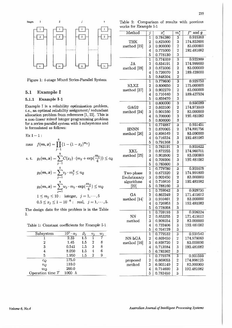
As one of the case studies of the nMIP prob-lem, we introduce some optimal reliability assign-ment/redundant allocation problems as complex systems. A complex system are usually decom-posed into . functional entities composed of units, subsystems, or components for the purpose of reliability. Combinatorial aspects of reliability analysis are connected to the components nei-ther purely in series nor purely in parallel. Ref [11, 17] contain detailed description of application of G A to the various reliability optimization prob-lems including complex systems. Figure 1 and 2 show such a multistage mixed system and a com-plex system considered in this paper, respectively. The objective is to determine the optimum level of component reliability and the number of re-dundant components at each subsystem simulta-neously while meeting the goal with a maximum reliability.

3 Proposed Method 3.1 NP/NN method We consider that the nMIP problem has no in-teger restrictions, because the neural network technique is an approximate method suitable for


232

a continuous decision variable values, i.e., we solve the non-linear programming (NP) problem [18, 19, 20]. Therefore, the nMIP problem should be relaxed to the NP problem as follows: NP:

t max f(m,x) = Lfj(mj,Xj)

j=l

t s. t. gi(m, x) = L9ij(mj, Xj) ::::: bi

j = l

i = 1,2, · ··,n my:::; mj :::; mf: real, j = 1, · · ·, t

xy :::; Xj :::; xf : real, j = 1, · · ·, t. Now, we construct the energy function based on the penalty method for solving the NP problem. The penalty method transforms a constrained optimization problem into an unconstrained one [18], so that the following energy function is ob-tained:

E(m, x , K) =- f(m, x) + ~ [~([bi- 9i(m, x)J-)2

t t + L)[mj- my]_)2 + L([mf- mj]-)2

j=l j=l

+ t.([x; - xfJ-)' + t. ([xf - x;]_)' ]·

where K > 0 is a penalty parameter, [bi- gi(m, x)]- = min{O, bi - gi(m, x)}, [mj]- = min{O,mj}, and [xj] - = min{O,xj}·

(1)

Minimizing the energy function leads to the sys-tem of ordinary differential equations as follows:

dmj = -t-£ [-of(m, x) + r.(t o[bi - 9i(m, x)J-dt omj i=l omj

x [bi- gi(m, x)J- + [mj - my]- [mf - mj]-)]

j = 1,2,···,t (2)

dxj = -J.L [-of( m , x) + "' ( t o[bi- gi(m, x)]-dt OXj i=l OXj

x [bi- gi(m, x)J- + [x j - xy] - [xf - Xj]-)] j = 1, 2, ... 't, (3)

where J.L ::_::: 0 is called learning parameter. We can obtain the optimal solutions (m0 , x 0 )

to the NP problem from the system of ordinary differential equations using by Runge-Kutta-Gill method [18].


3.2 Genetic Algorithms 3.2.1 Representation and Initialization

Now, we can consider the original nMIP prob-lem as a non-linear integer programming (niP) problem by fixing the optimal real decision vari-ables x 0 of the solutions (m0 , x 0 ) given by NN technique and by rounding the integer decision variables m 0 up to integer values mi.

Assuming that Vk denote the k-th chromosome in a population, the initial population is gener-ated within the below range of such genes in ini-tial solutions m I as follows:

Vk = [(mk1; xgl) · · · (mkj; xgJ) ···(mkt; xgt)l I I mkj - rev :::; mkj :::; mkj + rev

k = 1,2,·· ·,pop_size, j = 1,2,··· ,t,

where rev is the allowable width.

3.2.2 Evaluation Function

As an evaluation function for such chromosome, the following equation, eval ( v k; x 0 ) uses the scale di for describing the exceeded resource rate in the i-th system constraints (i = 1, 2, · · ·, n) (14]:

eval(vk; x 0 ) =

{ f(m , x 0 );

f(m , x 0 )(1 - o::::iEic di)/nc)i 9i(m, x 0 ) :::::: bi otherwise,

where

lc = {ilgi(m,x0 )>bi, i = l,···, n} d· = { 0; gi(m, x 0

) :::; bi t (gi(m, x 0)- bi)/bi; otherwise

ne is the number of exceeded system constraints.

3.2.3 Genetic Operators

• crossover: arithmetical crossover [10, 11, 13] . When we denote the two chromosomes se-lected randomly for crossover operation as v 1 and v 2 , the offspring will be

01 = lc·v1+(l - c)·v2J o2 = lc·v2+(l- c)·v1J ,

where la J is defined as maximum integer smaller than a given real number a, and c is a random number in range [0, 1 J.

• muta tion: uniform mutation (10 , 11]. For a chosen parent v , if its gene m 3 is randomly selected for mutation, the resulted offspring • 1 [ I l h I· IS v = m 1 m2 m 3 · · · mt, w ere m 3 IS a ran-dom (uniform probability distribution) value

· h" [ L Uj wit m m 3 , m3 .

Volume 6, No.4

• selection: The selection operator uses the roulette wheel and elitist approach [10, 11, 13] in order to obtain the variety of chromo-some because the arithmetic crossover tends to lose the variety of chromosomes in a pop-ulation while keeping the feasibility of chro-mosomes.

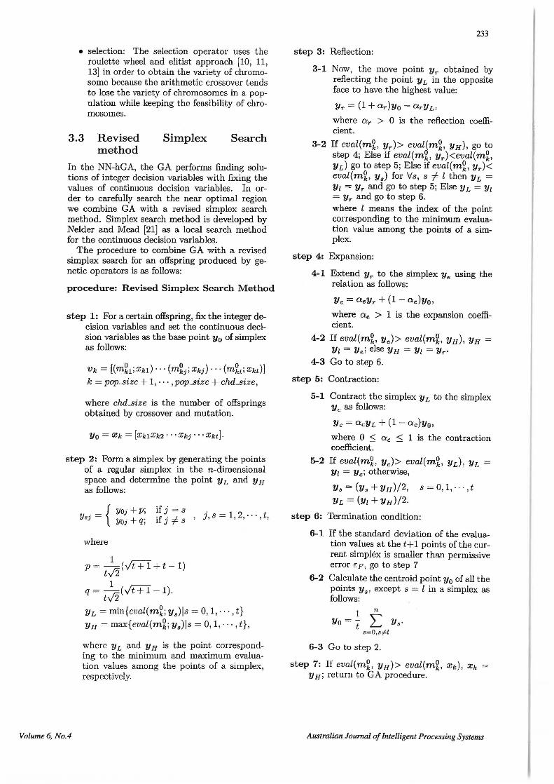
3.3 Revised Simplex Search method

In the NN-hGA, the GA performs finding solu-tions of integer decision variables with fixing the values of continuous decision variables. In or-der to carefully search the near optimal region we combine GA with a revised simplex search method. Simplex search method is developed by Nelder and Mead (21] as a local search method for the continuous decision variables.

The procedure to combine GA with a revised simplex search for an offspring produced by ge-netic operators is as follows:

procedure: Revised Simplex Search Method

step 1: For a certain offspring, fix the integer de-cision variables and set the continuous deci-sion variables as the base point y 0 of simplex as follows:

Vk = [(m~ 1 iXkl) · · · (m~jiXkj) · · · (m~tiXkt)] k = pop_size + 1, · · · ,pop_size + chd_size,

where chd..size is the number of offsprings obtained by crossover and mutation.

Yo = Xk = [xk1Xk2 · • · Xkj · · • Xkt]·

step 2: Form a simplex by generating the points of a regular simplex in the n-dimensional space and determine the point y L and y H as follows:

Volume 6, No.4

Ysj = {

where

YDj +p; Yoi + q;

if j = s if j =Is

p = 1;;:; ( Jt+I + t - 1)

tv2

q = 1;;:;(Vt+I -1). tv2

, j,s = 1,2,·· · ,t,

YL = min{eval(m~; Ys)ls = 0, 1, · · ·, t} YH = max{eval(m2; Ys)is = 0, 1, · · ·, t},

where YL and YH is the point correspond-ing to the minimum and maximum evalua-tion values among the points of a simplex, respectively.

233

step 3: Reflection:

3-1 Now, the move point Yr obtained by reflecting the point y L in the opposite face to have the highest value:

Yr = (1 + O:r)Yo- O:rYL,

where O:r > 0 is the reflection coeffi-cient.

3-2 If eval(m~, Yr)> eval(m~, YH), go to step 4; Else if eval(m~, Yr)<eval(mZ, Yd go to step 5; Else if eval(m~, Yr)< eval(mZ, y 8 ) for Vs, s :f;l then YL = Yt = Yr and go to step 5; Else YL = y 1 = Yr and go to step 6. where l means the index of the point corresponding to the minimum evalua-tion value among the points of a sim-plex.

step 4: Expansion:

4-1 Extend Yr to the simplex Ye using the relation as follows:

Ye = O:eYr + (1 - O:e)Yo, where O:e > 1 is the expansion coeffi-cient.

4-2 If eval(mZ, Ye)> eval(m~, YH), YH = Yt = Yei else YH = Yl = Yr·

4-3 Go to step 6.

step 5: Contraction:

5-1 Contract the simplex YL to the simplex y c as follows:

Ye= O:cYL + (1- O:c)Yo,

where 0 :<:; O:c :<:; 1 is the contraction coefficient.

5-2 If eval(m~, Ye)> eval(m~, Yd, YL Yt =Ye; otherwise,

Ys=(ys+YH)/2, s=0,1,···,t YL = (Yt + YH )/2.

step 6: Termination condition:

6-1 If the standard deviation of the evalua-tion values at the t+ 1 points of the cur-rent simplex is smaller than permissive error E: F, go to step 7

6-2 Calculate the centroid point y 0 of all the points y 8 , except s = l in a simplex as follows:

1 n

Yo = t L Ys· s=O,s,Pl

6-3 Go to step 2.

step 7: If eval(m~, YH )> eval(mZ, xk), Xk YH; return toGA procedure.


234

4 Overall Procedure of Pro-posed Method

In this section, we show the overall procedure of the hybridized genetic algorithm with a neural network technique and a simplex search method for solving nMIP problem.

procedure: NN-flcGA for nMIP

phase 1: Initial Search by NN Technique.

step 1: Set the initial values and the parameters of the NN technique: learning parameter J.L, penalty parameter "'• the initial values m;o) and x;o), step size ry, and permissive error c.

step 2: Perform the initial search by the NN technique:

2-1 Relax the nMIP problem into NP prob-lem by eliminating integer restrictions.

2-2 Construct the energy function E(m, x, "') for solving the NP problem.

2-3 Construct the system of ordinary dif-ferential equations from E(m, x, "')and then solve it by the Runge-Kutta method.

2-4 If lmj(tt + ry) - mj(tl)! <cor !xj(t2 + ry·6xj/6mi)-xj(t2)! < c·6xjj6mj, fix the continuous decision variables x 0

and round the integer decision variables m 0 up to integer values m 1, then go to phase 2.

phase 2: Optimal Search by hGA Technique.

step 1: Set the initial values and the parameters of the hGA: population size pop_size, crossover rate Pc, mutation rate PM, the maximum generation max_gen, and the allowable width rev, per-missive error eA, Eo, and max_idle, reflection coefficient Or, expansion coefficient ae, con-traction coefficient De·

step 2: Perform the optimal search by the hGA:

2-1 Generate initial population within the range of each genes with initial solutions mi.

2-2 Evaluation of chromosomes in initial population.

2-3 Recombine chromosomes by genetic op-erations and evaluate the offsprings.

2-4 If the standard deviation of the fitness values at the population in the cur-rent generation is larger than EA, go


to substep 2-5; Otherwise, adjust the continuous decision variables xZ (k = pop_size+1,pop_size+2, · · · ,pop_size+ chd_size) of offsprings by Revised Sim-plex Search method.

2-5 Select the chromosomes for the next generation and keep the best chromo-some.

step 3: Termination condition: If no significant improvement of fitness value is obtained during the max_idle times repe-tition or the generation arrives at max_gen, then terminate; Otherwise, go to substep 2-3.

5 Numerical Examples Here, we discuss the optimal reliability assign-ment/redundant allocation problem firstly intro-duced by Misra and Ljubojevic [1J. They consid-ered the problem of simultaneously determining optimal component reliabilities and optimal re-dundancy levels at t-subsystem of a series-parallel system subject to cost constraints as follows:

t max R(m, x) = fi {1- (1- Xj)'ni}

j=l t

s. t. 91 (m, x) = .2:C(xj) · (mj + exp( :j )) :::; CQ

j=l t

92(m, x) = .2:vj ·m]:::; VQ j=l

t

93(m, x) = .2:wi · mi · exp( :J) :::; WQ

j=l

1 :::; mj :::; 10: integer, j = 1, · · ·, t 0.5 :::; Xj :::; 1 - 10-6 : real j = 1, · · ·, t,

where Vj is the product of weight and volume per element at subsystem j, Wj the weight of each components at the subsystem j, and C(xj) the cost of each component with reliability Xj at sub-system j as follows:

-T C(x·)=a··(--).61 j=1,···t, 1 1 ln(xj)

where Oj, f3J are constants representing the phys-ical characteristic of each component at subsys-tem j, and T is the operating time during the component must not fail [1].

The system reliability f(m, x) is maximized subject to a cost constraint g1(m,x), product constraints 92(m, x), and g3 (m, x) of the volume and weight constraints for components.

Volume 6, No.4

Si ages 2 j

AA A A . . . . . . . . I o o o ' 0 t o

: : : ! . . ... ·: ~ . ... - ·: : 0 o o I 0 0 ' o

bJlJlJlJ Figure 1: t-stage Mixed Series-Parallel System

5.1 Example I 5.1.1 Example 1-1

Example I is a reliability optimization problem, i.e., an optimal reliability assignment/ redundant allocation problem from references [1, 22]. This is a non-linear mixed integer programming problem for a series-parallel system with 5 subsystems and is formulated as follows:

Ex I -1: 5

max f(m,x) = IT{1- (1-xj)m;} j=l

5

s. t. g1(m,x) = LC(xi) · (mj +exp(:j))::; CQ

j=l 5

g2(m,x) = LVJ ·m~::; VQ j=l

5 """ m· g3(m, x) = L...tWj • mi · exp( -f) ::; WQ j=l

1::; mi::; 10: integer, j = 1,···,5 0.5 ::; Xj ::; 1 - 10-6 : real, j = 1, · · · 1 5.

The design data for this problem is in the Table 1.

Table 1: Constant coefficients for Example I-1

Subsystem 1 2 3 4 5

CQ

VQ WQ

Operation time T

Volume 6, No.4

10" · Oj

2.33 1.45

0.541 8.050 1.950 175.0 110.0 200.0

1000 h

1.5 1 1.5 2 1.5 3 1.5 4 1.5 2

W j 7 8 8 6 9

235

Table 2: Comparison of results with previous works for Example I-1

Method j x; m:; f* and g 1 0.784380 3 0.915363

THK 2 0.825000 3 174.852606 method (23] 3 0.900000 2 83.000000

4 0.775000 2 192.481082 5 0.778130 3 1 0.774559 3 0.922909

JA 2 0.834191 3 174.999000 method [28] 3 0.873006 2 83.000000

4 0.720070 3 189.428000 5 0.848304 2 1 0.779600 3 0.929750

KLXZ 2 0.800650 2 175.000000 method [27] 3 0.902270 2 83.000000

4 0.710440 3 189.427524 5 0.859470 3 1 0.800000 3 0.930289

GAG2 2 0.862500 2 174.973500 method [24] 3 0.901560 2 83.000000

4 0.700000 3 192.481082 5 0.800000 3 1 0.774887 3 0.931451

HNNN 2 0.870065 2 174.891756 method [26] 3 0.898549 2 83.000000

4 0.716524 3 192.481082 5 0.791368 3 1 0.783191 3 0.931622

XKL 2 0.872255 2 174.960701 method (25] 3 0.903500 2 83.000000

4 0.709306 3 192.481082 5 0.785600 3 1 0.779780 3 0.931678

Two-phase 2 0.872320 2 174.991800 Evolutionary 3 0.902450 2 83.000000

algorithms 4 0.710810 3 192.481082 [22] 5 0.788160 3

1 0.759042 3 0.929735 GA 2 0.862249 2 171.415612

method (14] 3 0.910461 2 83.000000 4 0. 726953 3 192.481082 5 0.778058 3 1 0.759193 3 0.926224

NN 2 0.853255 2 171.415612 method 3 0.909354 2 83.000000

4 0.732406 3 192.481082 5 0.764129 3 1 0.779532 3 0.931542

NN-hGA 2 0.869450 2 174.978069 method [16] 3 0.898720 2 83.000000

4 0.713584 3 192.481082 5 0.79336·2 3 1 0.779378 3 0.931593

proposed 2 0.869053 2 174.998125 method 3 0.905140 2 83.000000

4 0.714600 3 192.481082 5 0.783450 3


236

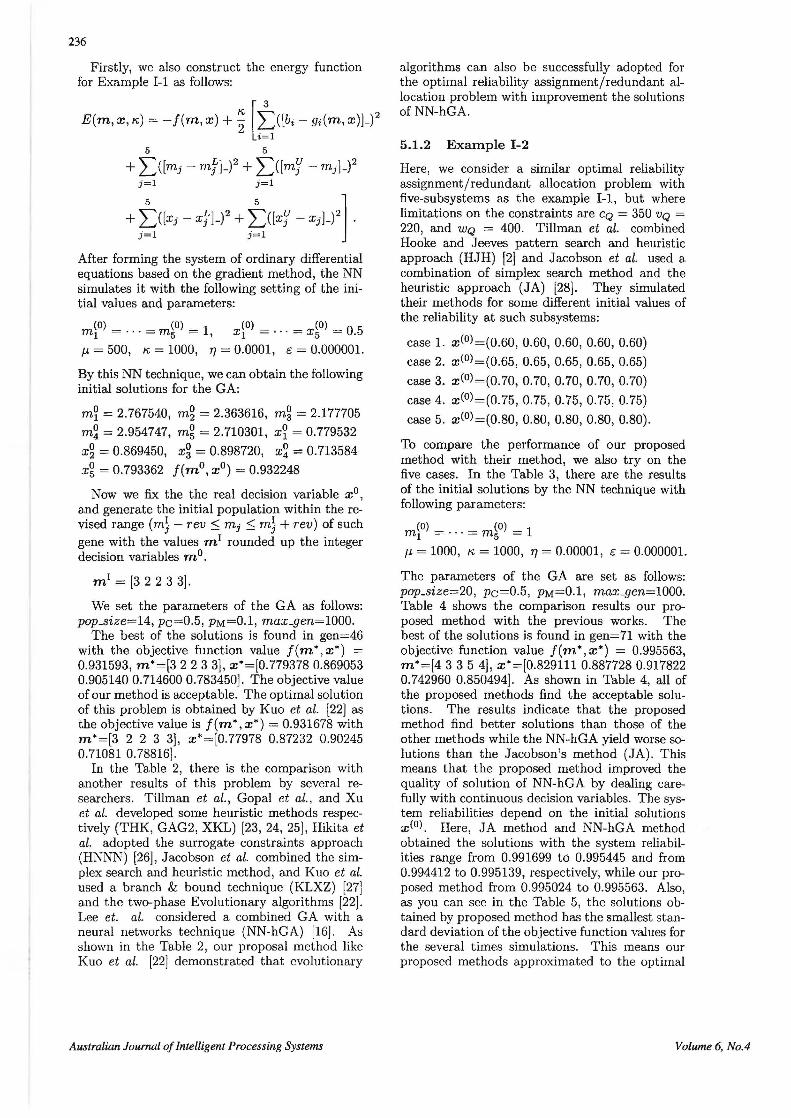
Firstly, we also construct the energy function for Example I-1 as follows:

E(m, x, K;) =-f(m, x) + ~ [t,([bi- gi(m, x)]-) 2

5 5

+ :l)[mj - mf]-)2 + L([mJ- mj]-)2 j =l j=l

+ t,((x; - xf]-)' + t,([xJ - x; )_)' ]· After forming the system of ordinary differential equations based on the gradient method, the NN simulates it with the following setting of the ini-tial values and parameters:

m~O) = · ·. = m~o) = 1, x~o) = · · · = x~o) = 0.5 J..L = 500, K; = 1000, 1/ = 0.0001, E: = 0.000001.

By this NN technique, we can obtain the following initial solutions for the GA:

m~= 2.767540, mg = 2.363616, mg = 2.177705 m~= 2.954747, mg = 2.710301, x~ = 0.779532 xg = 0.869450, xg = 0.898720, x~ = 0. 713584 xg = 0.793362 f(m0 , x 0 ) = 0.932248

Now we fix the the real decision variable x 0 , and generate the initial population within the re-vised range (m}- rev :::; mi :::; m}+ rev) of such gene with the values m 1 rounded up the integer decision variables m 0 •

m 1 = [3 2 2 3 3].

We set the parameters of the GA as follows: pop_size=14, pc=0.5, PM=0.1, max_gen=lOOO.

The best of the solutions is found in gen=46 with the objective function value f(m*,x*) = 0.931593, m*=[3 2 2 3 3], x*=[0.779378 0.869053 0.905140 0.714600 0.783450]. The objective value of our method is acceptable. The optimal solution of this problem is obtained by Kuo et al. [22] as the objective value is f(m*, x*) = 0.931678 with m*=[3 2 2 3 3], x*=[0.77978 0.87232 0.90245 0.71081 0.78816].

In the Table 2, there is the comparison with another results of this problem by several re-searchers. Tillman et al., Gopal et al., and Xu et al. developed some heuristic methods respec-tively (THK, GAG2, XKL) [23, 24, 25], Hikita et al. adopted the surrogate constraints approach (HNNN) [26], Jacobson et al. combined the sim-plex search and heuristic method, and Kuo et al. used a branch & bound technique (KLXZ) [27] and the two-phase Evolutionary algorithms [22]. Lee et. al. considered a combined GA with a neural networks technique (NN-hGA) [16]. As shown in the Table 2, our proposal method like Kuo et al. [22] demonstmted that evolutionary


algorithms can also be successfully adopted for the optimal reliability assignment/redundant al-location problem with improvement the solutions of NN-hGA.

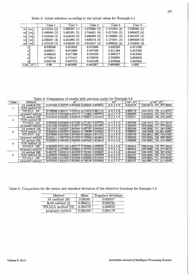
5.1.2 Example I-2

Here, we consider a similar optimal reliability assignment/redundant allocation problem with five-subsystems as the example I-1, but where limitations on the constraints are CQ = 350 VQ = 220, and WQ = 400. Tillman et al. combined Hooke and Jeeves pattern search and heuristic approach (HJH) [2] and Jacobson et al. used a combination of simplex search method and the heuristic approach (JA) [28]. They simulated their methods for some different initial values of the reliability at such subsystems:

case 1. x(0)=(0.60, 0.60, 0.60, 0.60, 0.60) case 2. x(0l=(0.65, 0.65, 0.65, 0.65, 0.65) case 3. x(0 )=(0.70, 0.70, 0.70, 0.70, 0.70) case 4. x(0l=(0.75, 0.75, 0.75, 0.75, 0.75) case 5. x(0)=(0.80, 0.80, 0.80, 0.80, 0.80).

To compare the performance of our proposed method with their method, we also try on the five cases. In the Table 3, there are the results of the initial solutions by the NN technique with following parameters:

m~o) = · · · = m~o) = 1 J..L = 1000, K; = 1000, 1/ = 0.00001, E: = 0.000001.

The parameters of the GA are set as follows: pop_size=20, pc=0.5, PM=0.1, max_gen=1000. Table 4 shows the comparison results our pro-posed method with the previous works. The best of the solutions is found in gen=71 with the objective function value f( m*, x*) = 0.995563, m*=[4 3 3 5 4], x*=[0.829111 0.887728 0.917822 0.742960 0.850494]. As shown in Table 4, all of the proposed methods find the acceptable solu-tions. The results indicate that the proposed method find better solutions than those of the other methods while the NN-hGA yield worse so-lutions than the Jacobson's method (JA). This means that the proposed method improved the quality of solution of NN-hGA by dealing care-fully with continuous decision variables. The sys-tem reliabilities depend on the initial solutions x<0l. Here, JA method and NN-hGA method obtained the solutions with the system reliabil-ities range from 0.991699 to 0.995445 and from 0.994412 to 0.995139, respectively, while our pro-posed method from 0.995024 to 0.995563. Also, as you can see in the Table 5, the solutions ob-tained by proposed method has the smallest stan-dard deviation of the objective function values for the several times simulations. This means our proposed methods approximated to the optimal

Volume 6, No.4

237

Table 3: Initial solutions according to the initial values for Example I-2

Case1 Case2 Case 3 Case4 CaseS m~ (mi) 4. 716353 (5) 4.098397 (4) 3.376969 (3) 3.575282 (4) 4.028903 ( 4) mg (m~) 3.496684 (3) 3.491381 (3) 3. 744621 ( 4) 3.017550 (3) 3.980422 (4) mg (m~) 3.234949 (3) 3.054033 (3) 2.886090 (3) 3.448904 (3) 3.062162 (3) m~ (mi) 4.309497 (4) 4.451986 (4) 4.838318 (5) 4.174501 (4) 4.086020 (4) mg (m~) 3.319148 (3) 3.658586 (4) 3.850317 (4) 4.000634 ( 4) 3.702956 (4)

X~ 0.838246 0.810016 0.875680 0.832330 0.811926 xg 0.862611 0.874699 0.847596 0.911184 0.817285 xg 0.890553 0.917409 0.931930 0.866177 0.913383 X~ 0.770814 0.771557 0.729224 0.783985 0.805603 X~ 0.881728 0.847273 0.841109 0.803949 0.847680

f (m*, x) 0.99 0.995496 0.995287 0.993998 0.994

Table 4: Comparison of results with previous works for Example I-2 Cases Method x~ m f( m*,ro* ) gi (m*,x")

JA method [28] [0.827409 0. 784737 0.872520 0.830837 0.882331 [4 54 3 3 0.991916 349.9570, 171, 377.0020 1 HJH method [2] - - - -

NN-!1vA [loj [0.838246 0.862611 O.!i90553 0.770814 O.!ilil T~8j [4 4 4. 4_;j j U.!J94412 (349.5623, 178, 372.4797) propose« method [0.828b lo o.tsoJ1U2 0.9162,~5 0.724832 0.892749] 44 35 3 0.995393 (349.9995, 1lM, 375.7742) JA method (28] [0.833848 0.821861 0.833218 0.790871 0.884984 44443 0.994611 (349.9630, 178, 372.4800)

2 HJJ1 method [2] - - - -NN-hvA [16j 0.810016 0.874699 0.917409 0. 771557 0.857273 4434 4 0.994758 346.7012, 171, 377.0018

proposed method 0.8412J6 0.846835 0.915471 O.Tf9iJt! 0.851855 4 4 344 0.995382 [::!49.!:1!:192, 171, 377.0011! J A method (28J 0.811087 0.833297 0.807690 0.837787 0.880092 44533 0.991699 349.9890, 177, 397.9760

3 _t:I J_Ji mettlo<l L2J 0.900000 O.MOOUU 0.856000 0. 750000 0.850000 [3 4 4 4 4 0.993657 (349.9668, 185,381.5250) NN-hvA [16j 0.875680 O.t5475l:l6 0.931930 0.729224 0.841101 [3 4 3 54 0.995139 [::!4!:1.8842, 2UU, :184.811!5

proposed method U.!i29111 O.M87728 O.l:ll'f!i22 0.742!:160 0.850494 43354 0.99556::! [34!:1.9998, 193, <SMU.2l:l63 JA method [28] 0.823863 0.805535 0.848400 0.809436 0.879018 44443 0.993990 349.9800, 178, 372.4800

4 HJH method [21 - - - -NN-hvA [1tij 0.8::!2330 0.!:111184 0.8ti6Hl 0."(1!3985 0.803949 43444 0.994544 [349.!i732, 178, 377.0011!)

proposed method 0.829746 0.8l:I7UOI! O.!itit!682 0.7!i7035 0.8374M 4 34 44 0.!:1!!50£4 [350.0UUU, 17li, 377.0U l li ) JA method [28] 0.821791 0.843210 0.925390 0. 792268 0.839437 44344 0.995445 349.9830, 188, 397.9760)

5 H JH method [2] 0.850000 0.863000 0.902000 0.700000 0.900000 44353 0.994767 [349.9935, 193, 375.7740) NN-hvA [16] 0.811926 0.817285 0.913383 0.805603 0.847680 44344 0.995028 [349.9804, 171, ::S77.UU18)

proposed method O.!i43446 O.!i::S5::S7U 0.921t!UO 0. 790746 0.829268 4 4 3 44 O.l:ll:l542c( 349.9961, 171, <S77.U018)

Table 5: Comparison for the means and standard deviation of the objective functions for Example I-2

Method Mean Standard deviation JA method [28] 0.93532 0.003317 HJH method [2] 0.994212 0.000785

NN-hGA method [16] 0.994776 0.000618 proposed method 0.995358 0.000179

Volume 6, No.4 Australian Journal of Intelligent Processing Systems

238

more steady than other method. For the mean of objective functions , the proposed method yielded better results than the other methods, too.

Figure 2: Complex System

5.1.3 Example 11

Here, we consider an optimal reliability assign-ment/redundant allocation problem with com-plex system as Example II [26]. The reliability of the complex system is maximized subject to the same constraints with Example I-1 and is de-signed as follows:

f(m,x) = R1(m,x)R2(m,x) + (1- R1(m, x)R2(m, x))

R3(m, x)R4(m, x) + (1- R2(m, x))(l- R3(m, x))

R1(m,x)R4(m, x)R5(m, x) + (1- R1(m, x))(l- R4(m, x))

R2(m, x)R3(m, x)R5(m, x).

Recently, related to this complex system, Rocco et al. proposed a new approach using cellular evo-lutionary strategies (CESs), with concepts from cellular automata [29] . The authors solved the optimal reliability assignment/redundant alloca-tion problem with a complex system of CESs and obtained better results than those of the HNNN method [26] . For this numerical example, we compare the results of NN technique, GA, NN-hGA and proposed method with those of CESs and HNNN method.

Firstly, we also construct the energy function for Example II. After forming the system of ordi-nary differential equations based on the gradient method, the NN simulates it with the following setting of the initial values and the parameters:

m~o) = . .. = m~o) = 1, x~o) = ... = x~o) = 0.5

f.L = 105 , "'= 105 , TJ = 10- 5 , E = w-7 .

By this NN technique, we can obtain the following initial solutions for the GA:

m~ = 2.867540, mg = 2.725413, mg = 2.431750


m~ = 2.876247, mg = 1.720139, x~ = 0.793164 xg = 0.823214, xg = 0.899624, x~ = 0.720264 xg = 0.820714 f(m 0 , x 0 ) = 0.999959.

Table 6: Comparison of results with previous works for Example II

Method j X~ m~ f* and g 1 0.791309 3 0.999780

HNNN 2 0.815125 3 174.875982 method (26) 3 0.909668 2 83.000000

4 0.720610 3 189.427525 5 0.819419 2 1 0.765518 3 0.999817

GA 2 0.845692 3 174.675900 method (14) 3 0.901221 2 105.000000

4 0.709195 4 198.439500 5 0.758174 1 1 0.813146 3 0.999830

NN 2 0.877363 3 174.997800 method 3 0.855659 3 78.000000

4 0.746221 2 195.534600 5 0.726681 2 1 0.834787 3 0.999871

CES 2 0.846385 3 172.527554 method [29) 3 0.851430 3 92.000000

4 0.717269 3 195.735230 5 0.717758 1 1 0.812638 3 0.999851

NN-hGA 2 0.861748 3 174.913100 method (16} 3 0.899969 2 83.000000

4 0.701032 3 189.427500 5 0.747798 2 1 0.812638 3 0.999886

proposed 2 0.861748 3 174.989223 method 3 0.899969 3 92.000000

4 0.701032 3 195.735233 5 0.747798 1

Now we fix the the continuous decision variable x 0 , and generate the initial population within the allowable range (m} - rev :S m1 :S m}+ rev) of such gene with the values m 1 rounding up the integer decision variables m 0 .

m 1 = [3 3 2 3 2].

We set the parameters of the hGA as follows: pop_si ze=14, pc=0.5, PM=0.1 , max _gen=1000. The best of the solutions is found in gen=142 with the objective function value f(m*,x*) = 0.999886, m*=[3 3 3 3 1], x *=[0.812638 0.861748 0.899969 0.701032 0.747798] .

Table 6 shows the comparison results the fitness values of proposed method with those of previous works. Our proposed method finds better solu-tions than those of the other methods when NN-hGA yield worse solutions than those of CESs. That means the proposed method improve the quality of chromosome by incorporat ing revised simplex search method.

Volume 6, No.4

Table 7: Constant coefficients for Example Ill

j 1 2 3 4 5 6 7 8 9 Cj 2 2 4 1 2 3 4 3 4

W j 2 8 4 4 3 4 7 4 7 j 10 11 12 13 14

Cj 4 3 2 3 5 CQ 130 Wj 5 5 4 5 6 WQ 170

5.2 Example Ill As the third numerical experiment, we consider a large-scale nMIP model for a series system con-sisting of 14 subsystems from reference [14]. This optimal reliability assignment/ redundant alloca-tion problem is formulated as follows: Ex III:

14

max f(m,x) =IT {1- (1- Xj)m;} j=1

14

s. t. 91(m,x) = L::Cj · mj ~ CQ j=1 14

92(m,x) = L:wj · mj::; WQ j =1

mj ;:::: 0: integer, j = 1, · · ·, 14 0.5 ::; Xj :::; 1 - 10-6 : real, j = 1, · · · , 14,

where Cj is the coefficient of the cost of each com-ponent at subsystem j and wi is the weight of each components at the subsystem j. Table 7 shows the design data for this problem.

Before forming the system of ordinary differen-tial equations, we construct the energy function by Eq. (1).

The NN technique searched the following initial solutions for the GA: m~ = 2.048893, mg = 2.585703, m~= 2.183538 m~ = 2.781218, m~ = 2.300556, mg = 2.702270 m~ = 2,582632, mg = 2.407727, m8 = 2.879093 m~0 = 2.615179, m~1 = 3.021275, m~2 = 1. 751168 m~3 = 2.413700, m~4 = 2.030302 , x~ = 0.969320 xg = 0.999425, X~ = 0.980382, X~ = 0.997304 X~ = 0.986699, xg = 0.996496, X~= 0.994787 xg = 0.990682, x8 = 0.998052, x~0 = 0.995321 x~1 = 0.998785, x~2 = 0.999944, x~3 = 0.990865 ~4 = 0.969366, f(m, x 0 ) = 0.997985

with the following setting of the initial values and the parameters:

m~o) = · · · = m~~) = 0, x~O) = · · · = x~~ = 0.5 IL = 1ooooo, "' = wooo, rt = w-s, c = w-6

.

After fixing the the real decision variables x 0 , and rounding up the integer decision variables m 0

m 1 = [2 3 2 3 2 3 3 2 3 3 3 2 2 2],

Volume 6, No.4

239

we run the GA with the following parameters: pop_size=10, Pc=0.4, PM=0.1, max_gen=1000. The best of the solutions is found in gen=216 with the objective function value f (m*, x*) = 0.0.999735, m*=[4 2 3 4 3 4 2 3 3 2 2 1 2 2], x*=[0.995641 0.995626 0.998293 0.978990 0.998237 0.998220 0.998098 0.988653 0.993597 0.988670 0.998098 0.999990 0.996145 0.990880]. The objective value of our method is acceptable.

Table 8 shows the comparison of results with the GA [14], NN and NN-hGA [16]. As shown in the table, our proposed method finds better solutions the GA and NN and NN-hGA for the large-scale optimal reliability assignment/ redun-dant allocation problem.

Table 8: Comparison of results with previous works for Example III

GA method 14] NN method f(m*, x*)=0.970015 !(m*, x* )=0.993750

9t(m*, x*)=119 91(m*, x*)=l06 92(m*, x*)=170 92(m*, x*)=166

j mj xj mj X~ 1 0.910000 3 0.962983 3 2 0.950000 2 0.984365 2 3 0.920000 3 0.989832 2 4 0.850000 3 0.957343 3 5 0.940000 3 0.962634 3 6 0.980000 2 0.961392 3 7 0.910000 2 0.995230 1 8 0.810000 4 0.980102 2 9 0.960000 2 0.985425 2 10 0.850000 3 0.963321 3 11 0.940000 2 0.989035 2 12 0.790000 4 0.937726 4 13 0.990000 2 0.964342 3 14 0.950000 2 0.959726 3 NN-hGA method [16] proposed method f(m*, x*)=0.997985 f(m*, x* )=0.999735

91(m*,x*)=109 g1(m*, x*)=l07 g2(m*, x*)=169 92(m*, x*)=170

j mj x j m j x j 1 0.969320 5 0.995641 4 2 0.999425 2 0.995626 2 3 0.980382 3 0.998293 3 4 0.997304 2 0.978990 4 5 0.986699 2 0.998237 3 6 0.996496 2 0.998220 4 7 0.994787 1 0.998098 2 8 0.990682 3 0.988653 3 9 0.998052 3 0.993597 3 10 0.995321 2 0.988670 2 11 0.998785 2 0.998098 2 12 0.999944 4 0.999990 1 13 0.990865 3 0.996145 2 14 0.967366 3 0.990880 2


240

6 Conclusions When there is an option to select both compo-nent reliability and redundancy level at all or some subsystems of a system, then the reliabil-ity optimization problem is formulated as a non-linear mixed integer programming (nMIP) prob-lem. Recently, we proposed the hybridized ge-netic algorithm with neural network technique (NN-hGA) to solve the nMIP problem. NN-hGA solves the relaxed non-linear programming prob-lem from nMIP using by a neural network (NN) technique, and then used the genetic algorithm (GA) to search the optimal solutions among in-teger search space. In this paper, we combined NN-hGA with the simplex search method as a lo-cal search technique to deal with continuous de-cision variables, in order to more carefully search the near optimal region in GA procedure.

Devising the initial values of GA and hybridiz-ing the revised simplex search method made for GA improve the quality of solutions by control-ling effectively the continuous decision variable. Numerical comparison experiments demonstrated the efficiency of the proposed method for solv-ing the nMIP problems. Example I stated that the NN-hGA not only has the robustness under various conditions of the problem but can also be successfully adopted for the optimal reliabil-ity assignment/redundant allocation problem. In Example II and Example Ill, we confirm the ef-ficiency of the proposed method on a complex system or a large-scale nMIP model of the opti-mal reliability assignment/ redundant allocation problem.

Acknowledgments This research was supported by the International Scientific Research Program, the Grant-in-Aid for Scientific Research (No.l0044173: 1998.4-2001.3) by the Ministry of Education, Science and Cul-ture, the Japanese Government.

References [1] W . Kuo, V. R. Prasad, F . Tillman, and C. L. Hwang

(2000) Optimization Reliability Design: Fundamen-tals and Applications, Cambridge Univ. Press.

[2J F A Tillman, C L Hwang, and W Kuo (1980) Opti-mization of Systems Reliability, Dekker.

[3] M Gen (1975) Reliability optimization by 0-1 pro-gramming for a system with several failure modes, IEEE Trans. on Rel., R-24, 206-210, also in [?], pp. 252-256.

[4] A Land and A Doig (1960) An automatic method for solving discrete programming problems, Econo-metrics, 2, 497-520.

[5] R Dakin (1965) A tree-search algorithm for mixed integer programming problems, Comput. J., 8, 250-255.


[6J M P Kamat and L Mesquita (1994) Nonlinear mixed integer programming, In Advances in Design Opti-mization (H Adeli, Ed .) , pp. 174-193.

[7] T L Morin and R S Marsten (1976) An algorithm for non-linear knapsack problems, Management Sci-ence, 22, 1147-1158.

[8J R S Marsten and T L Morin (1978) A hybrid approach to discrete mathematical programming, Mathematical Programming, 4, 21-40.

[9] H L Li ( 1992) An approximate method for local optima for non-linear mixed integer programming problems, Comput. f1 Ops. Res., 19 (5), 435-444.

[10] M Gen and R Cheng (2000) Genetic Algorithms and Engineering Optimization, John Wiley & Sons, New York.

(11] M Gen and R Cheng (1997) Genetic Algorithms and Engineering Design, John Wiley & Sons, New York.

[12] D E Goldberg (1989) Genetic Algorithms in Search, Optimization & Machine Learning, Addison Wesley.

[13] Z Michalewicz (1994) Genetic Algorithms + Data Structures= Evolution Programs, 2nd ed., Springer-Verlag.

(14] T Yokota, M Gen, and Y Li (1996) Genetic algorithm for non-linear mixed integer programming problems and its applications, Comput. f1 Indust. Engg., 30 (4), 905-917.

[15] R Ostermark (1999) Solving nonlinear con-convex trim loss problem with a genetic hybrid algorithm, Comput. f1 Ops. Res., 26, 623-635.

[16] C. Y. Lee, M. Gen and W. Kuo (2001) Reliability op-timization design using hybridized genetic algorithm with a neural network technique, IEICE Trans. Fun-damental, E84-A (2), 627-637.

[17] M Gen and J Kim (1999) A GA-based approach to reliability design, In Evolutionary Design by Com-puters, Kalifornia (Peter J Bentley, Ed.), pp. 191-218, Morgan Kaufmann .

[18] A Cichocki and R Unbehauen (1994) Neural Net-works for Optimization and Signal Processing, John Wiley & Sons, New York.

[19] M Gen, K Ida, and H Omori (1996) Method for solv-ing non-linear integer programming problem using neural network, Proc. of JIMA Spring Meeting., pp. 175-176 (in Japanese) .

[20] D Gong, M Gen, G Yamazaki , and W Xu (1995) Neural network approach for general assignment problem, Proc. of IEEE Inter. Conf. on Neural Net-works, pp. 1861-1866.

[21] S. S. Rao (1996) Engineering Optimization, 2nd ed., John Wiley & Sons, New York.

[22] V R Prasad and W Kuo (1997) Redundancy allo-cation ina power cooling system, Technical Report, Dept. of I. E. Engg., Texas A & M University.

[23] F A Tillman, C L Hwang, and W Kuo (1977) De-termining component reliability and redundancy for optima l system reliablility, IEEE Trans . on Rel., R-26 (3) , 162-165.

[24] K. Gopal, K. I<. Aggarwal, and J. S. Gupta (1978) An improved a lgorithm for reliability optimization , IEEE Trans . Relia6., R-27 (5), 325-328.

Volume 6, No.4

[25] Z Xu, W Kuo, and H Lin (1990) Optimization limits in improving system reliability, IEEE Trans. on Re!., 39 (1), 51-60.

[26) MY Hikita, Y Nakagawa, K Nakashima, and H Nar-ihisa (1992) Reliability optimization of system by a surrogate-constraints algorithm, IEEE Trnas. on Rel., 41 (3), 473-280.

[27] W Kuo, H Lin, Z Xu, and W Zhang (1987) Relia-bility optimization with the Lagrange multiplier and branch and bound technique, IEEE 11-ans. on Re!., R-36 (5), 624-630.

[28] D W Jacobson and S A Arora (1996) Simultaneous allocation of reliability & redundancy using simplex search, IEEE Proc. of Annual Reliavility and Main-tainability System, pp. 243-250.

[29] C. M. Rocco S., A. Miller, J. Moreno, and N. Car-rasquero (2000) A cellular evolutionary approach ap-plied to reliability optimization of complex systems, Proc. Annual Reliability and Maintainability Sym-posium, 210-215.

241

Volume 6, No.4 Australian Journal of Intelligent Processing Systems

a hybrid g a to solve non-linear mixed integer programming

Documents