a hybrid generic algorithm for dynamic data mining in...
TRANSCRIPT

International Journal on Data Science and Technology 2016; 2(6): 62-71
http://www.sciencepublishinggroup.com/j/ijdst
doi: 10.11648/j.ijdst.20160206.12
ISSN: 2472-2200 (Print); ISSN: 2472-2235 (Online)
A Hybrid Generic Algorithm for Dynamic Data Mining in Investment Decision Making
Kangzhi Yu1, Yufang Li
2, Zhengying Cai
1, *
1College of Computer and Information Technology, China Three Gorges University, Yichang, China 2College of Economics and Management, China Three Gorges University, Yichang, China
Email address:
[email protected] (Kangzhi Yu), [email protected] (Yufang Li), [email protected] (Zhengying Cai) *Corresponding author
To cite this article: Kangzhi Yu, Yufang Li, Zhengying Cai. A Hybrid Generic Algorithm for Dynamic Data Mining in Investment Decision Making. International
Journal on Data Science and Technology. Vol. 2, No. 6, 2016, pp. 62-71. doi: 10.11648/j.ijdst.20160206.12
Received: October 16, 2016; Accepted: November 8, 2016; Published: December 9, 2016
Abstract: To solve the risks and uncertainty problem in investment decision-making, a dynamic data mining architecture is
introduced here. First, the investment decision-making process is examined and the involved risks are analyzed. Accordingly,
dynamic data mining architecture is proposed here with the dynamic search ability of the generic algorithm. Second, a hybrid
algorithm with dynamic learning ability is submitted to overcome the local minima problem prevalent in dynamic data mining.
Whenever new data are generated, the data mining algorithm can dynamically collect the original input data without any
reconstruction, to realize the dynamic update for investment decision-making. Last, an example is illustrated to verify the
proposed model, and the solution provides us an effective model to improve the robustness of investment decision-making
under risk environment.
Keywords: Dynamic Data Mining, Investment Decision, Hybrid Genetic Algorithms, Risk Management
1. Introduction
The investment decision-making problem is very
important in modern economy, but the risks in investment
environment increased the difficulty to make a right decision.
To solve this risk problem, data mining is introduced in all
decision making support systems. Zanin (2016) made a deep
analysis on the combination of complex network analysis and
data mining, and describes how to extract information from
the complex system, and finally create a new compact
quantitative representation in combining complex networks
and data mining [1]. Heinecke (2016) showed us the
optimization of data mining algorithms to solve the
regression and classification problems in a broad data set in
Data mining on vast data sets as a cluster system benchmark
[2]. Garcia (2016) summarized the most influential data
preprocessing algorithms, the impact of each algorithm is
discussed, and the current research and further research is
reviewed in Tutorial on practical tips of the most influential
data preprocessing algorithms in data mining [3]. An
approximate method for dynamic maintenance of objects and
attributes was proposed by Chen (2015) in a
decision-theoretic rough set approach for dynamic data
mining [4]. Chen (2015) discussed the production and
development of the logistics fee policy in toll policy for load
balancing research based on data mining in port logistics. It
studied the impact of the charges on the consumer's choice of
logistics, and even the choice of departure time [5].
Moreover machine learning and artificial intelligence are
applied in data mining to improve its performance. A set of
unsupervised machine learning techniques was proposed and
applied by Gajowniczek (2015) in data mining techniques for
detecting household characteristics based on smart meter data
to reveal the specific usage patterns [6]. Morro (2015)
achieved a similar search of the data with respect to different
pre stored categories in ultra-fast data-mining hardware
architecture based on stochastic computing [7]. Zheng (2015)
conducted a systematic survey, the main research on the
trajectory of data mining, to provide a panoramic view of the
field, as well as the scope of its research topics in trajectory
International Journal on Data Science and Technology 2016; 2(6): 62-71 63
data mining with an overview [8]. Li (2015) published a
paper entitled distributed data mining based on deep neural
network for wireless sensor network, and this paper proposed
a distributed data mining method based on deep neural
network (DNN), divided by the deep neural network into
different levels, and put them into the sensor [9]. Boland
(2015) discussed the future development trends of business
intelligence and data mining in business intelligence, data
mining, and future trends [10]. Li (2014) researched
integrates three data mining techniques, k- means clustering,
decision tree and neural network to predict the travel time of
non-recurrent congested highways in a data mining based
approach for travel time prediction in freeway with
non-recurrent congestion [11].
With the further development of the complexity of human
activities, the diversity of information, began showing
explosive growth, in order to fully grasp the new information
on the dynamic data source (database, sequence data,
streaming data etc.) data mining becomes inevitable. An
advanced process management method, called "program
tree" (PT), was proposed for radio frequency identification
data mining by Kwon (2014) in a real time process
management system using RFID data mining [12]. Itzama
(2014) introduced a new association model of time series
data mining, which is based on gamma classifier in a novel
associative model for time series data mining [13]. The
classification of proton transfer events using artificial neural
networks was evaluated in pattern recognition and data
mining software based on artificial neural networks applied
to proton transfer in aqueous environments by Tahat (2014)
[14]. Hassani (2014) described a thorough review of the
published work on the date of data mining applications in
official statistics, and identifies the technology that has been
explored in data mining and official statistics form the past,
the present to the future [15]. The main focus of the work
described in experimental analysis on the normality of pi, E,
phi, root 2 using advanced data-mining techniques by
Xylogiannopoulos (2014) was to examine whether the
well-known mathematical constants of phi, E, phi, and root 2
are normal figures [16]. A survey by Tsai (2014) first
discussed the Internet of Things, and then briefly reviewed
the "Internet of Things" and "Internet of Things data mining"
function. Finally, the future development trend of this field is
discussed [17]. Mirco (2014) published a paper entitled with
big mobile data mining from good or evil [18]. Xu (2014)
discussed the privacy security issues under the big data in his
information security in big data from privacy and data
mining [19]. Wu (2014) proposed a kind of theorem, the
characteristics of the big data revolution, put forward a large
data processing model, from the point of view of data mining
in data mining with big data [20]. Lima(2016) put forward a
hybrid neural evolutionary algorithm (NEA) using a compact
indirect encoding scheme (IES) said its genotype, but also by
the genotype and the automatic construction of modular,
hierarchical recursive neural network in optimization of
neural networks through grammatical evolution and a genetic
algorithm [21].
To diminish the risk and uncertainty problem, dynamic
data mining is especially presented. Yuregir (2016) used
modern data mining methods (SOM and k- mean) and the
official statistics of the city cluster according to their
consumption characteristics, welfare level and growth rate,
and compare them with the help of renewable resource
potential rapid mine in solar energy validation for strategic
investment planning via comparative data mining methods
with an expanded example within the cities of Turkey [22]. A
decision-theoretic rough set approach for dynamic data
mining by Chen (2015) described an approximate dynamic
maintenance method for objects and attributes, and the
decision theory of rough set theory (DTRS) is proposed [23].
Composite rough sets for dynamic data mining was proposed
by Zhang (2014), with a composite relationship of multiple
different types of attributes, and the upper approximation and
lower approximation of the composite rough set were
re-defined [24]. The dynamic data mining and traditional data
warehouse based on data mining very different from
traditional data mining is mining based on historical data,
extract the knowledge hidden in them, and dynamic data
mining is in the past, present and future in the development of
knowledge extraction process.
This paper presents a solution for dynamic data mining
with high precision. It is focused on the state feedback and
dynamic adjustment of parameters, and then a set of
investment decision rules, and a set of neural network
weights will be gotten. For each network, a genetic algorithm
is used to foster a more healthy weight and update its
feedback rule. Genetic algorithm is used to optimize the
weights of neural network, which solves the problem of slow
convergence speed of the traditional algorithm.
In any given generation, data mining starts from a fixed
initial state, and then updates the relevant parameters and
weights with the addition of more dynamic data. Because it is
important to look for a fixed feedback rule and the same
neural network weights, so it is to avoid the dependence on
the initial conditions to accelerate the learning speed of
genetic algorithm from the initial state to do data mining,
thus.
In essence, every data mining algorithm will update the
investment data with the new and more accurate and
excellent neural network. Initially, GA starts a searching
based on the initial data set. However, with the continuous
data and updating for each investment decision-making
network training, any other policy rules will gradually be
made to achieve the most appropriate weight. According to
the updated weights, each decision maker can better predict
the best return on an investment plan.
The structure of this paper is as follows. In the 2nd section,
some basic concepts of investment decision making and
dynamic data mining are briefly discussed. In the 3rd section,
a brief introduction is given on the neural network and
genetic algorithm, and then a hybrid algorithm of GA
optimized BP is proposed. In the 4st section, a simple test of
the performance of the hybrid algorithm is made based on the
background of the investment decision example.
64 Kangzhi Yu et al.: A Hybrid Generic Algorithm for Dynamic Data Mining in Investment Decision Making
2. Dynamic Data Mining for Investment
Decision Making
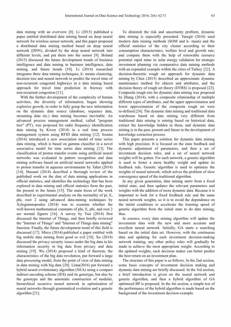
2.1. Investment Decision-Making Process
The investment decision-making with risks is a complex
process, as shown in figure 1. To determine the investment
target is the premise of investment decision-making, in the
specific investment objectives. To further develop the
investment direction, the dynamic data mining system was
then used, from the dynamic DDS (dynamic data source)
where extracted data were analyzed according to the results of
the analysis, to the investment plan where the feasibility of the
scheme evaluation was demonstrated in detail. The
investment plan is mainly to evaluate the investment risk and
return analysis, thus determining the reliability of investment
decision. The investment plan can adjust the original decision
according to the changing environment and needs, making the
investment decision more scientific and reasonable.
Figure 1. Investment decision-making process.
In the investment decision-making process, it is important
to solve the dynamic acquisition of effective data and
dynamic processing of them.
As the current time point T, there is a number )( *'' RTT ∈ ,
in the DDS before the '~ TT moments when the formation
of all the id composed of the data set will become a
historical data set, denoted as oldD .
As the current time point T, existing number )( *'' RTT ∈ ,
in the DDS from the '~ TT time to the time T is to generate
all the id composing of the data set to become the current
data set, denoted as currentD .
As the current time point T, existing number )( *'' RTT ∈ ,
in the DDS after the T moments when the formation of all the
id compose of the data set to become the subsequent data
set, denoted as newD
.
2.2. Dynamic Data Mining Architecture
With the further development of the complexity of human
activities, the diversity of information began showing
explosive growth. In order to fully grasp the new information
on the dynamic data source (database, sequence data,
streaming data etc.), data mining becomes inevitable. The
dynamic data mining and traditional data warehouse based on
data mining are very different from each other. Traditional
data mining is to mine data based on historical data, extract
the knowledge hidden in them, whereas dynamic data mining
is based on the past, present and future data in the
development of knowledge extraction process.
Dynamic data mining is mainly embodied to dynamically
extracted data from DDS (dynamic data source) for analysis
to find out the knowledge and planning, and it is more
popular for the enterprises and institutions or management

International Journal on Data Science and Technology 2016; 2(6): 62-71 65
departments to provide decision-making plan. The dynamic
data mining process can be divided into dynamic data
acquisition, data processing, data mining, the evaluation
process of dynamic data mining. The key is to solve the
problems of dynamic acquisition of subsequent data sets and
dynamic processing.
The data sources used in investment decision making will
be divided into three data sets. First, historical data set for
long-term investment information, and its updating time is
generally a quarter or year. Second, updating data set for the
real-time data is related to investment projects, and these data
will fine tune the weights for the data network, where the
updating time is in accord with the importance of the new
data and can be automatically adjusted by the decision
makers or by customs. Third, the buffered data set is a
collection of rough and original data. The hybrid algorithm
proposed in this thesis will use the dynamic data source to be
continuous to optimize the proposed method with the
survival of the fittest structure according to the actual needs
of the problem, to obtain a set of rules for investment
decision and investment decision support.
Dynamic data mining (DDM) is mainly embodied in it can
dynamically extract data from DDS (dynamic data source)
for further analysis to find out the knowledge and planning,
to provide decision-making plan.
The following is the system structure of dynamic data
mining:
Figure 2. Dynamic data mining architecture.
As we can see, in DDS, according to the data di ( i for the
data identification number, *i Z∈ ), the generation time is
divided into the window size of τ (τ for the time period,
and ' *( )T n Zτ γ= ∈ and 1γ ≥ ) with the data segment Dk,
where each data segment is for a data window, and τ is for
the data threshold value.
For an integer x ,
*( , 1)x n n Z nτ= ∈ ≥ , for a time T, a
data set 1 2{ , ,....., }nD D D D= in the window size of the x
window SW can be gotten every τ time to move forward the
location of the s data window size, where the window SW can
be called as a sliding window.
2.3. Dynamic Data Processing with General Neural
Network Algorithm
The neural network can be used for classification,
clustering, and prediction. Historical data can be acquired to
form a certain amount of historical data, then the network can
learn the hidden knowledge in the data through training. In
this case, some characteristics of the dynamic data processing
is to find some further problems, and the corresponding
evaluated can be used to train the neural network.
If you are using a simple BP algorithm to train the neural
network, there will be some problems, such as, BP learning
algorithm is very slow. The possibility of failure of network
training is great. The application examples of problems are
difficult to solve the contradiction between the scale of
problem and the scale of the network. This involves the
relationship between the possibility and feasibility of network
capacity, namely learning complexity. The selection of
network structure is not a unified and complete theoretical
guidance, and it is general only selected by experience.
Therefore, the selection of neural network structure is known
as a kind of art. But the network directly affects the structure of
neural network and many extended properties. Therefore, the
application of how to choose the suitable network structure is
an important and difficult problem. The new sample has effect
in the success of the network learning, and describes the
characteristics of each number of input samples must be the
same, including the contradiction between the network
prediction ability and training ability. In general, for ability
training, if the prediction ability is poor, to a certain extent
with the ability to improve training, the prediction ability will
be improved. But this trend has some limits, when it reaches a
limit, the training ability and the predictive ability will
decrease, which is called over-regularization phenomenon. At
this time, the network learning is too much for the details of
the sample to reflect the sample containing rules.
Although the BP network has been widely used, it also has
some shortcomings, mainly including the following aspects.
Firstly, the learning rate is fixed, so the convergence speed is
slow and a longer training time is often required. For some
complex problems, the BP algorithm may requires too much
for the training time, mainly due to the learning rate is too
small to be used to change the learning rate or adaptive
learning rate for improvement. Secondly, the BP algorithm
can make convergence to a certain value, but it does not
guarantee its minimum value in the global error level,
because the gradient descent method may produce a local
66 Kangzhi Yu et al.: A Hybrid Generic Algorithm for Dynamic Data Mining in Investment Decision Making
minimum. For these problems, it can not be easily solved by
additional momentum methods. Thirdly, in the network
number of hidden layers and the unit layer selection there is
no theoretical guidance, and it is generally based on
experience or through repeated experiments for sure.
Therefore, the network often has great redundancy, to a
certain extent, also increases the burden of network learning.
Finally, the learning and memory of the network are unstable.
That is to say, if the learning samples increase, the trained
network will be needed to start training, so there will be no
memory of previous weights and the threshold can not be
predicted. However, the classification or clustering needs a
better weighting preservation.
3. Hybrid General Algorithm for
Dynamic Data Mining
In this section, genetic algorithm (GA) is selected to train the
neural network for the following reasons. First, compared with
the gradient descent method, the genetic algorithm does not use
gradient information. Therefore, it does not require the existence
of continuity and derivation of the objective functional or state
transfer function. The only limitation is that it is bounded. Of
course, it can be applied to a larger class of problems. Second,
the genetic algorithm is a global search algorithm, based on the
historical data set from start, and then makes some adjustments
according to the updated data, which can guarantee the
convergence of approximate solutions to global optimal domain
space and relatively better development by genetic operators.
The gradient descent method, on the other hand, requires the
gradient information and may stay in a local optimum or not,
which depends on the initial parameters.
Compared with the traditional data mining technology, neural
network provides a more flexible solution. The genetic
algorithm is select to train the neural network, because the
genetic algorithm guarantees the convergence to an approximate
global optimum no matter what the initial parameter values are.
Another feature of GA is that it has parallelism.
3.1. Introduction of Neural Network Algorithm and Genetic
Algorithm
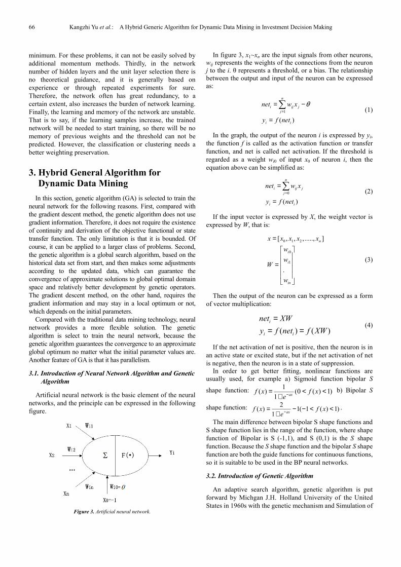
Artificial neural network is the basic element of the neural
networks, and the principle can be expressed in the following
figure.
Figure 3. Artificial neural network.
In figure 3, x1~xn are the input signals from other neurons,
wij represents the weights of the connections from the neuron
j to the i. θ represents a threshold, or a bias. The relationship
between the output and input of the neuron can be expressed
as:
1
( )
n
i ij j
j
i i
net w x
y f net
θ=
= −
=
∑ (1)
In the graph, the output of the neuron i is expressed by yi,
the function f is called as the activation function or transfer
function, and net is called net activation. If the threshold is
regarded as a weight wi0 of input x0 of neuron i, then the
equation above can be simplified as:
0
( )
n
i ij j
j
i i
net w x
y f net
=
=
=
∑ (2)
If the input vector is expressed by X, the weight vector is
expressed by W, that is:
0 1 2
0
1
[ , , ,....., ]
.
n
i
i
in
x x x x x
w
wW
w
=
=
(3)
Then the output of the neuron can be expressed as a form
of vector multiplication:
)()( XWfnetfy
XWnet
ii
i
===
(4)
If the net activation of net is positive, then the neuron is in
an active state or excited state, but if the net activation of net
is negative, then the neuron is in a state of suppression.
In order to get better fitting, nonlinear functions are
usually used, for example a) Sigmoid function bipolar S
shape function: )1)(0(1
1)( <<
+= − xf
exf
ax b) Bipolar S
shape function: )1)(1(11
2)( <<−−
+= − xf
exf
ax.
The main difference between bipolar S shape functions and
S shape function lies in the range of the function, where shape
function of Bipolar is S (-1,1), and S (0,1) is the S shape
function. Because the S shape function and the bipolar S shape
function are both the guide functions for continuous functions,
so it is suitable to be used in the BP neural networks.
3.2. Introduction of Genetic Algorithm
An adaptive search algorithm, genetic algorithm is put
forward by Michgan J.H. Holland University of the United
States in 1960s with the genetic mechanism and Simulation of
International Journal on Data Science and Technology 2016; 2(6): 62-71 67
natural biological evolution theory and the GA algorithm. Its
theoretical support comes from Darwin's theory of evolution.
The theory is based on the process of biological evolution in
nature, animal and plant species where every generation keeps
on evolving in the constant survival process of the fittest to
adapt to the new environment. Through the genetic algorithm
of group encoding, selection, crossover and mutation
operations, individual screening are performed to find a high
degree of individual to be retained in the community. By the
elimination of the fitness difference of individual, no
generation inherits a same generation of information of its
parents, and is better than the previous generations to meet the
conditions. So far, it is to realize the simulation of the natural
survival law of the fittest in natural selection.
The general genetic algorithm consists of four parts: coding
mechanism, fitness function, genetic operator and control
functions.
1) Coding mechanism
Genetic algorithm is not to discuss the research object
directly, but through some kind of coding mechanism, where
the object is given by the specific symbols according to a
certain sequence. As the biological heredity is from the
chromosomes, and the chromosome is a string of genes.
Character set consists of 0 and 1, the code is two strings, and the
general GA is not affected by this restriction. In an optimization
problem, a string is corresponding to a possible solution and a
string class is interpreted in classification as a rul. This is also an
important reason for the wide application of GA.
2) Fitness function
Survival of the fittest is the principle of natural evolution. In
the genetic algorithm, the fitness function is used to describe
the degree of adaptation of each individual. To an optimization
problem, the fitness function is often chosen as the objective
function. The introduction of the fitness function is designed
according to their fitness to assess the individual comparison,
and determine the extent of the pros and cons, in order to carry
out the survival of the fittest genetic operation.
3) Genetic operator
Genetic operators including the selection of reproduction
operator, crossover operator, mutation operator, respectively,
to simulate the natural biological reproduction, mating and
gene mutation processes.
4) Control parameters
In the actual operation of the genetic algorithm, it is needed
to determine the string length of the solved string to improve
the effect of the selection. Here, the string length is denoted as
L; the group size is denoted as size. crossover rate, that is, the
probability of crossover operator is denoted as Pc; mutation
rate is denoted as Pm, that is, the probability of the
implementation of the compiler.
3.3. Optimization of Neural Network by Genetic Algorithm
Genetic algorithm is an adaptive search algorithm of global
optimization probability, which simulates the genetic and
evolutionary process of biological in the natural environment.
Traditional genetic algorithm has many advantages, but there
are still some problems, this paper proposes an improved
genetic algorithm, based on the standard genetic algorithm to
improve the 4 points:
1) Floating point code;
2) Uniform generation of initial population;
3) Using dynamic selection operation;
4) Adaptive adjustment of 0t
cP =
and
t
mP . (
t
cP is the
exchange of probability of first generation. t
mP
is the
mutation probability of the t generation, t is a time
factor.
The expression of the adaptive formula is:
max min
min min
exp( / ),
,
t
m m mt
m t
m m m
P t T P PP
P P P
η • − >= ≤
(5)
In the formula, maxmP is the largest mutation probability,
minmP is the minimum one, η is a constant, t is an algebra
and T is the maximum genetic algebra.
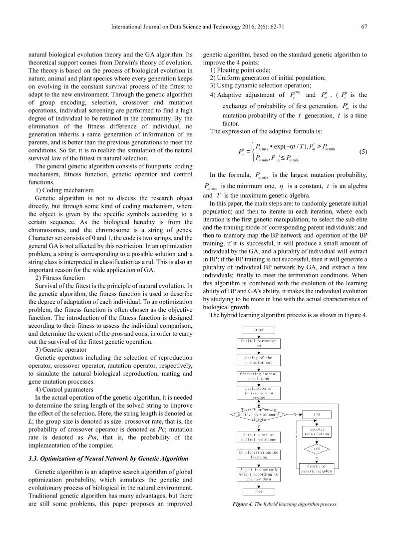
In this paper, the main steps are: to randomly generate initial
population; and then to iterate in each iteration, where each
iteration is the first genetic manipulation; to select the sub elite
and the training mode of corresponding parent individuals; and
then to memory map the BP network and operation of the BP
training; if it is successful, it will produce a small amount of
individual by the GA, and a plurality of individual will extract
in BP; if the BP training is not successful, then it will generate a
plurality of individual BP network by GA, and extract a few
individuals; finally to meet the termination conditions. When
this algorithm is combined with the evolution of the learning
ability of BP and GA's ability, it makes the individual evolution
by studying to be more in line with the actual characteristics of
biological growth.
The hybrid learning algorithm process is as shown in Figure 4.
Figure 4. The hybrid learning algorithm process.
68 Kangzhi Yu et al.: A Hybrid Generic Algorithm for Dynamic Data Mining in Investment Decision Making
As a three layer BP neural network, n is the number of input
nodes, p is the number of hidden nodes, m is the number of
output nodes. The activation function of the input layer to the
hidden layer is S type, and the activation function of the
hidden layer to the output layer is a linear function. Given a
training set, the input mode is 1 2[ , , , , , ]q dI I I I… … , so the
corresponding target output is 1 2[ , , , , , ]q dO O O O… … , it is
said a total of d training samples, where I is a
n-dimensional vector, O is a m dimension of the desired
output and the actual output vector, and the vector H , is
available between the input and output of the network
relationship:
k
p
j
n
ijiijjkk rIWfVH ++••= ∑ ∑
= =1 1
][ θ (6)
Among them, ijW
is the connection weight between node
i in the implicit layer and node j in the input layer, jkV
is the threshold value of the node j in the hidden layer.
For the connection weights between the node j in the
hidden layer and the node k in the output layer, kr is the
threshold of the node k in third output layer, kH is the
actual output of node k in output layer. According to the
error between the actual output vector and the target output
vector, a least square error function is defined.
∑∑= =
−=d
q
m
i
qi
qi HOrVWM
1 1
2)(),,,( θ (7)
Among them, qi
qi OO , is indicated in the first training
sample q training with the desired output and the actual
output of the node i of the output layer.
The least squares error function can be used to describe the
performance of the neural network, and the optimization
objective function is to optimize a network output and the
minimum square error. And the requirement of network
structure should be as simple as possible, namely the network
nodes and their connections should be as least as possible.
In order to combine genetic algorithm with neural network,
there is
∑∑= =
−+=
d
q
m
i
qi
qi HO
rVWF
1 1
2)(1
1),,,( θ
(8)
The error function of the network output is the smallest
when the adaptive degree of the offspring is the maximum. Its
optimization function is:
( )rVWF ,,,max θ (9)
, , ,m p p n p n
W R V R R r Rθ× ×
⊂ ⊂ ⊂ ⊂ is the range of the
variables in the formula.
The coefficient weights and threshold values are encoded
by floating point numbers, and the string length is
length n p p p m m= × + + × + ( n is the number of input
nodes, p is the number of hidden nodes, m is the number
of output nodes). The code is concatenated into a long string
according to a certain order, corresponding to [ , , , ]W V rθ .
4. Example Application and Performance
Analysis
4.1. Example Explanation
Here is an example for dynamic data mining in investment
decision making, as shown in Table 1. As can be seen from
the table 1, the company in the three years of 2012-2014, the
flow rate and speed ratio increased slightly, the asset liability
ratio showed a downward trend, which shows the company's
solvency has increased. Accounts receivable turnover and
inventory turnover rate have growth trend, which show that
the company's sales situation has a good trend.
Table 1. Investment selection parameters.
Index parameter 2012 2013 2014
Flow rate 1.92 1.91 1.99
Quick ratio 1.26 1.27 1.28
Asset liability ratio 0.52 0.49 0.47
Accounts receivable turnover rate 11.46 13.55 14.23
Inventory turnover 5.66 6.58 6.62
Turnover ratio of total assets 2.27 2.29 2.25
Net asset interest rate 33.88% 32.36% 30.35%
Return on shareholders' equity 64.86% 63.81% 57.18%
Net sales rate 17.85% 14.23% 13.43%
Flow rate = current assets / current liabilities
Speed ratio = quick assets / current liabilities
Asset liability ratio = Total Liabilities / total assets
Accounts receivable turnover rate of credit = net income /
average accounts receivable
Inventory turnover = cost of sales / inventory balance
Total asset turnover = sales / total assets
Net profit margin = net profit / total assets
Return on shareholders' equity = net profit / total
stockholders' equity.
Net profit margin = net profit / net profit
However, the company's total asset turnover rate has not
changed much. It is worth noting that the company's three
profitability indicators are declining. According to the above
analysis, although the solvency of the company enhanced, but
the asset turnover rate has not accelerated, and the company's
profitability is declining. Therefore, it is important to strengthen
the sales work, strictly control costs and expenses, in order to
reverse the trend of declining profitability of the company.
International Journal on Data Science and Technology 2016; 2(6): 62-71 69
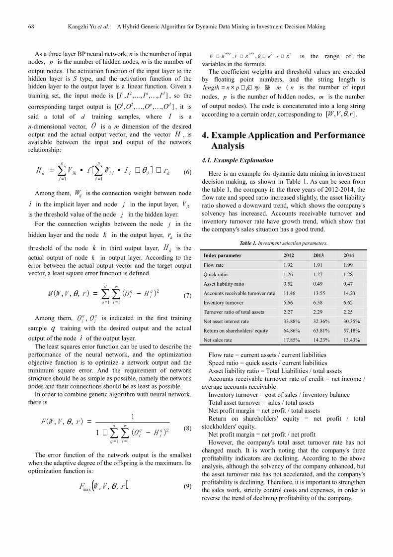
4.2. Results Analysis
The curve of mean square error is shown in figure 5. The
training of a total of 800 times, with a time of 7 seconds, the
average variance of the training time is 0.01, the mean
variance of the training time is 0.001. The following figure for
the neural network in training 800 times shows the
performance of the indicators, where the three lines shown in
the figure, are the actual training indicators, the best indicators
of line and target line, respectively.
Figure 5. Mean square error.
It can be seen from the figure that the convergence rate is
very fast in the initial stage of training, but in the later period
of training, the convergence rate is obviously slowed down.
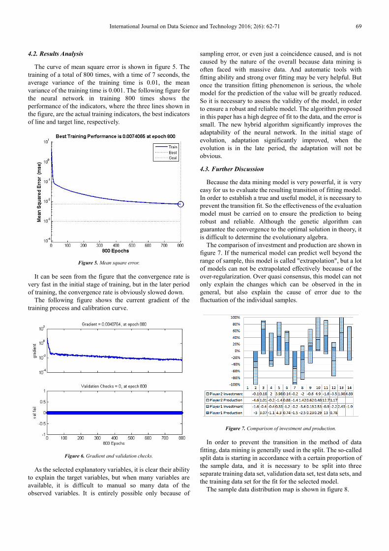
The following figure shows the current gradient of the
training process and calibration curve.
Figure 6. Gradient and validation checks.
As the selected explanatory variables, it is clear their ability
to explain the target variables, but when many variables are
available, it is difficult to manual so many data of the
observed variables. It is entirely possible only because of
sampling error, or even just a coincidence caused, and is not
caused by the nature of the overall because data mining is
often faced with massive data. And automatic tools with
fitting ability and strong over fitting may be very helpful. But
once the transition fitting phenomenon is serious, the whole
model for the prediction of the value will be greatly reduced.
So it is necessary to assess the validity of the model, in order
to ensure a robust and reliable model. The algorithm proposed
in this paper has a high degree of fit to the data, and the error is
small. The new hybrid algorithm significantly improves the
adaptability of the neural network. In the initial stage of
evolution, adaptation significantly improved, when the
evolution is in the late period, the adaptation will not be
obvious.
4.3. Further Discussion
Because the data mining model is very powerful, it is very
easy for us to evaluate the resulting transition of fitting model.
In order to establish a true and useful model, it is necessary to
prevent the transition fit. So the effectiveness of the evaluation
model must be carried on to ensure the prediction to being
robust and reliable. Although the genetic algorithm can
guarantee the convergence to the optimal solution in theory, it
is difficult to determine the evolutionary algebra.
The comparison of investment and production are shown in
figure 7. If the numerical model can predict well beyond the
range of sample, this model is called "extrapolation", but a lot
of models can not be extrapolated effectively because of the
over-regularization. Over quasi consensus, this model can not
only explain the changes which can be observed in the in
general, but also explain the cause of error due to the
fluctuation of the individual samples.
Figure 7. Comparison of investment and production.
In order to prevent the transition in the method of data
fitting, data mining is generally used in the split. The so-called
split data is starting in accordance with a certain proportion of
the sample data, and it is necessary to be split into three
separate training data set, validation data set, test data sets, and
the training data set for the fit for the selected model.
The sample data distribution map is shown in figure 8.
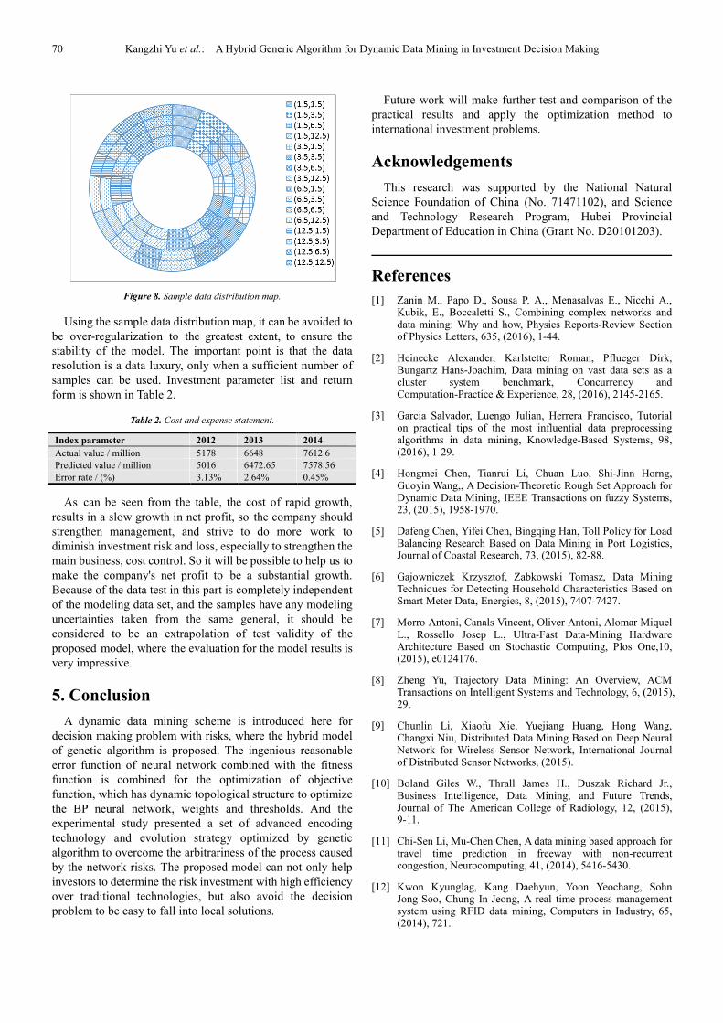
70 Kangzhi Yu et al.: A Hybrid Generic Algorithm for Dynamic Data Mining in Investment Decision Making
Figure 8. Sample data distribution map.
Using the sample data distribution map, it can be avoided to
be over-regularization to the greatest extent, to ensure the
stability of the model. The important point is that the data
resolution is a data luxury, only when a sufficient number of
samples can be used. Investment parameter list and return
form is shown in Table 2.
Table 2. Cost and expense statement.
Index parameter 2012 2013 2014
Actual value / million 5178 6648 7612.6
Predicted value / million 5016 6472.65 7578.56
Error rate / (%) 3.13% 2.64% 0.45%
As can be seen from the table, the cost of rapid growth,
results in a slow growth in net profit, so the company should
strengthen management, and strive to do more work to
diminish investment risk and loss, especially to strengthen the
main business, cost control. So it will be possible to help us to
make the company's net profit to be a substantial growth.
Because of the data test in this part is completely independent
of the modeling data set, and the samples have any modeling
uncertainties taken from the same general, it should be
considered to be an extrapolation of test validity of the
proposed model, where the evaluation for the model results is
very impressive.
5. Conclusion
A dynamic data mining scheme is introduced here for
decision making problem with risks, where the hybrid model
of genetic algorithm is proposed. The ingenious reasonable
error function of neural network combined with the fitness
function is combined for the optimization of objective
function, which has dynamic topological structure to optimize
the BP neural network, weights and thresholds. And the
experimental study presented a set of advanced encoding
technology and evolution strategy optimized by genetic
algorithm to overcome the arbitrariness of the process caused
by the network risks. The proposed model can not only help
investors to determine the risk investment with high efficiency
over traditional technologies, but also avoid the decision
problem to be easy to fall into local solutions.
Future work will make further test and comparison of the
practical results and apply the optimization method to
international investment problems.
Acknowledgements
This research was supported by the National Natural
Science Foundation of China (No. 71471102), and Science
and Technology Research Program, Hubei Provincial
Department of Education in China (Grant No. D20101203).
References
[1] Zanin M., Papo D., Sousa P. A., Menasalvas E., Nicchi A., Kubik, E., Boccaletti S., Combining complex networks and data mining: Why and how, Physics Reports-Review Section of Physics Letters, 635, (2016), 1-44.
[2] Heinecke Alexander, Karlstetter Roman, Pflueger Dirk, Bungartz Hans-Joachim, Data mining on vast data sets as a cluster system benchmark, Concurrency and Computation-Practice & Experience, 28, (2016), 2145-2165.
[3] Garcia Salvador, Luengo Julian, Herrera Francisco, Tutorial on practical tips of the most influential data preprocessing algorithms in data mining, Knowledge-Based Systems, 98, (2016), 1-29.
[4] Hongmei Chen, Tianrui Li, Chuan Luo, Shi-Jinn Horng, Guoyin Wang,, A Decision-Theoretic Rough Set Approach for Dynamic Data Mining, IEEE Transactions on fuzzy Systems, 23, (2015), 1958-1970.
[5] Dafeng Chen, Yifei Chen, Bingqing Han, Toll Policy for Load Balancing Research Based on Data Mining in Port Logistics, Journal of Coastal Research, 73, (2015), 82-88.
[6] Gajowniczek Krzysztof, Zabkowski Tomasz, Data Mining Techniques for Detecting Household Characteristics Based on Smart Meter Data, Energies, 8, (2015), 7407-7427.
[7] Morro Antoni, Canals Vincent, Oliver Antoni, Alomar Miquel L., Rossello Josep L., Ultra-Fast Data-Mining Hardware Architecture Based on Stochastic Computing, Plos One,10, (2015), e0124176.
[8] Zheng Yu, Trajectory Data Mining: An Overview, ACM Transactions on Intelligent Systems and Technology, 6, (2015), 29.
[9] Chunlin Li, Xiaofu Xie, Yuejiang Huang, Hong Wang, Changxi Niu, Distributed Data Mining Based on Deep Neural Network for Wireless Sensor Network, International Journal of Distributed Sensor Networks, (2015).
[10] Boland Giles W., Thrall James H., Duszak Richard Jr., Business Intelligence, Data Mining, and Future Trends, Journal of The American College of Radiology, 12, (2015), 9-11.
[11] Chi-Sen Li, Mu-Chen Chen, A data mining based approach for travel time prediction in freeway with non-recurrent congestion, Neurocomputing, 41, (2014), 5416-5430.
[12] Kwon Kyunglag, Kang Daehyun, Yoon Yeochang, Sohn Jong-Soo, Chung In-Jeong, A real time process management system using RFID data mining, Computers in Industry, 65, (2014), 721.

International Journal on Data Science and Technology 2016; 2(6): 62-71 71
[13] Lopez-Yanez Itzama, Sheremetov Leonid,Yanez-Marquez Cornelio, A novel associative model for time series data mining, Pattern Recognition Letters, 41, (2014), 23-33.
[14] Tahat Amani, Marti Jordi, Khwaldeh Ali, Tahat Kaher, Pattern recognition and data mining software based on artificial neural networks applied to proton transfer in aqueous environments, Chinese Physics B, 23, (2014).
[15] H. Hassani, G. Saporta and E. S. Silva, Data Mining and Official Statistics: The Past, the Present and the Future, Big Data, 2, (2014), 34-43.
[16] Xylogiannopoulos, Konstantinos F., Karampelas Panagiotis, Alhajj Reda, Experimental Analysis on the Normality of pi, e, phi, root 2 Using Advanced Data-Mining Techniques, Experimental Mathenatics, 23, (2014), 105-128.
[17] Chun-Wei Tsai, Chin-Feng Lai, Ming-Chao Chiang, Laurence T. Yang, Data Mining for Internet of Things: A Survey, IEEE Communications Surveys and Tutorials, 16, (2014), 77-97.
[18] Musolesi Mirco, Big Mobile Data Mining: Good or Evil?, IEEE Internet Computing, 18, (2014), 78-81.
[19] Lei Xu, Chunxiao Jiang, Jian Wang, Jian Yuan, Yong Ren,
Information Security in Big Data: Privacy and Data Mining, IEEE Access, 2, (2014), 1149-1176.
[20] Xindong Wu, Xingquan Zhu, Gong-Qing Wu, Wei Ding, Data Mining with Big Data, IEEE Transactions on Knowledge and Data Engineering, 26, (2014), 97-107.
[21] C. Lima, M. Lidio, O. Limao, C. Roberto and M. Roisenberg, Optimization of neural networks through grammatical evolution and a genetic algorithm, Expert Systems with Applications, 56, (2016), 368-384.
[22] O. H. Yuregir and C. Sagiroglu, Solar Energy Validation for Strategic Investment Planning via Comparative Data Mining Methods: An Expanded Example within the Cities of Turkey, International Journal of Photoenergy, 8506193, (2016).
[23] Hongmei Chen, Tianrui Li, Chuan Luo, Shi-Jinn Horng, Guoyin Wang, A Decision-Theoretic Rough Set Approach for Dynamic Data Mining, IEEE Transactions on fuzzy Systems, 23, (2015), 1958-1970.
[24] Junbo Zhang, Tianrui Li, Hongmei Chen, Composite rough sets for dynamic data mining, Information Sciences, 257, (2014), 81-100.