a hybrid naval hydrodynamic scheme … hybrid naval hydrodynamic scheme based on an efficient...
TRANSCRIPT
A HYBRID NAVAL HYDRODYNAMIC SCHEME BASED ON AN EFFICIENT
LATTICE BOLTZMANN METHOD COUPLED TO A POTENTIAL FLOW SOLVER
Christopher O’Reilly1,2, Stephan Grilli1, Jason Dahl1, Christian F. Janssen3, Amir Banari3, J.J. Shock1,
Micha Uberrueck3
1University of Rhode Island, Department of Ocean Engineering, Narragansett, Rhode Island, USA 2Navatek LTD, South Kingstown, Rhode Island, USA
3Fluid Dynamics and Ship Theory Inst., Hamburg University of Technology, Germany
This paper details the development of a 3D coupled approach between a boundary element method potential flow
model, for the large- to near-field scale, and a Navier-Stokes model in the near-field, based on a velocity and pressure
decomposition approach. We focus on the development of a new viscous solver, intended for this coupling, which is
based on the Lattice Boltzmann Method. The solver uses a large eddy simulation of the turbulence and volume of fluid
free surface capturing method. The method is validated by simulating an advancing surface piercing hydrofoil for
which there are both published and new laboratory experiments; hence, this case represents a rigorous benchmark for
the proposed free surface solver.
KEY WORDS Lattice Boltzmann; Finite Difference Lattice Boltzmann; Hybrid
Viscous Methods
INTRODUCTION
The simulation of large ship motions and resistance in steep
waves is typically performed using linear or nonlinear potential
flow solvers usually based on higher-order Boundary Element
Methods (BEM), with semi-empirical corrections introduced to
account for viscous/turbulent effects. However in some cases
viscous effects near the ship’s hull and breaking waves and wakes
need to be accurately modeled to capture the relevant physics.
Navier-Stokes (NS) solvers can and have been used to model
these problems, but they are computationally expensive and often
too numerically dissipative to model wave propagation over long
distances.
Here, we detail the development of a 3D coupled approach,
based on a perturbation approach (i.e., a velocity and pressure
decomposition; Harris and Grilli, 2012), between a BEM
nonlinear potential flow model, referred to as Numerical Wave
Tank (NWT), simulating the large- to near-field scales, and a NS
model simulating the near-field. Developments of the NWT,
which is optimized with a Fast Multipole Method (FMM), and its
more recent optimization on large parallel clusters have been
reported elsewhere (e.g., Grilli et al., 2010; Harris et al., 2014).
In this paper, we focus on the development and validation of an
efficient free-surface NS solver, to be used in this coupling
method, based on the Lattice Boltzmann Method (LBM; e.g.,
d’Humieres et al., 2002; Janssen, 2010; Janssen et al., 2010). In
the LBM, turbulence is modeled by a Large Eddy Simulation
(LES; Krafczyk et al., 2003) and the free surface is captured using
the volume of fluid (VOF) method. While the NWT based on a
FMM-BEM is optimized to achieve nearly linear scaling on large
CPU clusters (Harris et al., 2014), the LBM is implemented on a
massively parallel General Purpose Graphical Processor Unit
(GPGPU) co-processor; other work has shown that LBM models
can achieve a very high efficiency on such hardware (over 100
million node updates per second on a single GPGPU; e.g.,
Janssen, 2010; Janssen et al., 2013; Banari et al., 2014).
We first describe the two-way unsteady perturbation
coupling approach being used to solve fluid body interaction
problems (Janssen et al., 2010). Next, we detail the development
of the LBM model and present results of a simple validation
application of the coupling approach for a viscous oscillatory
Boundary Layer (BL; Janssen, 2010). We then further validate
the LBM based on experimental results alongside a comparison
with results of the potential flow model Aegir.
The LBM has proved to be accurate and efficient for simulating
a variety of complex fluid flow and fluid-structure interaction
problems (e.g., Banari et al., 2014; Janssen et al., 2010, 2013).
Hence, in the context of the field decomposition approach, the
combination of a LBM only applied to the near-field, with a fast
BEM potential flow solver applied to the entire domain, in a
hybrid approach, LBM has the potential for a much increased
computational efficiency relative to traditional CFD approaches
in which a NS solver is applied over the entire domain. This was
already demonstrated, based on other less optimized models, by
Reliquet et al. (2014). One reason for high efficiency of the LBM
is the inherent locality of its collision-propagation operators,
allowing for linear scalability for parallel computing on GPGPU
units. Furthermore, recent developments in LBM modeling allow
for the accurate and stable simulation of high Reynolds number
flows (e.g., Banari et al., 2014).
Once the relevance of the coupling approach is demonstrated for
an oscillatory wave BL, the LBM scheme is validated through an
advancing surface piercing hydrofoil test case, representing a
rigorous benchmark for the free surface solver. Such a foil has all
the characteristics and is thus a simpler proxy for a ship with a
more complex hullform. A large set of new well-controlled
A HYBRID NAVAL HYDRODYNAMIC SCHEME BASED ON AN EFFICIENT LATTICE BOLTZMANN METHOD COUPLED TO A
POTENTIAL FLOW SOLVER
2
O’Reilly et al.
laboratory experiments for an advancing vertical, surface-
piercing, foil with NACA 0012 profile was performed at the
University of Rhode Island, to serve as a rigorous validation of
the various numerical models, as well as their coupling approach.
Here, the measured free surface geometry and velocity field
around the foil are compared with model simulations for a range
of Froude numbers.
DECOMPOSITION COUPLING APPROACH Let us first illustrate the decomposition-coupling approach in a
simple case of viscous flow and consider the NS equations for an
incompressible, isothermal, Newtonian fluid: 𝜕𝑢𝑖
𝜕𝑥𝑖= 0 (1)
𝜕𝑢𝑖
𝜕𝑡+
𝜕
𝜕𝑥𝑗(𝑢𝑖𝑢𝑗 +
𝑝
𝜌𝛿𝑖𝑗 − 𝜈
𝜕𝑢𝑖
𝜕𝑥𝑗) = 0 (2)
Where 𝑢𝑖 and p are the water velocity and dynamic pressure,
respectively, in a fluid of density 𝜌 and kinematic viscosity 𝜈. We
introduce a decomposition of the flow into the sum of an inviscid
component and defect or perturbation flow component.
𝑢𝑖 = 𝑢𝑖𝐼 + 𝑢𝑖
𝑃 (3)
𝑝 = 𝑝𝐼 + 𝑝𝑃 (4)
When only considering the inviscid flow fields, Eqs. (1) and (2)
yield Euler’s equations:
𝜕𝑢𝑖
𝐼
𝜕𝑥𝑖= 0 (5)
𝜕𝑢𝑖
𝐼
𝜕𝑡+
𝜕
𝜕𝑥𝑗(𝑢𝑖
𝐼𝑢𝑗𝐼 +
𝑝𝐼
𝜌𝛿𝑖𝑗) = 0 (6)
Inserting Eqs. (3) and (4) into Eqs. (1) and (2), and applying Eqs.
(5) and (6), the remaining terms represent the governing
equations for the perturbation field
𝜕𝑢𝑖
𝑃
𝜕𝑥𝑖= 0 (7)
𝜕𝑢𝑖
𝑃
𝜕𝑡+
𝜕
𝜕𝑥𝑗(𝑢𝑖𝑢𝑗 − 𝑢𝑖
𝐼𝑢𝑗𝐼 +
𝑝𝑃
𝜌𝛿𝑖𝑗 − 𝜈
𝜕𝑢𝑖
𝜕𝑥𝑗) = 0 (8)
Based on Kelvin’s theorem, Eqs. (5) and (6) can be exactly solved
with a potential flow solver, when the flow is started from a state
of rest, which provides the inviscid flow fields to force Eqs. (7)
and (8). The latter equations can be directly solved with a
standard NS solver (e.g., as in Harris and Grilli, 2012 and
Reliquet et al., 2014). However here, as detailed later, Eqs. (7)
and (8) will be solved with a LBM in which the inviscid forcing
terms will be treated as volume forces in the collision operator.
In the context of an unsteady ship simulation, viscous forcing
terms are typically insignificant far from the body, where the flow
can accurately be modeled in a potential flow solver. As the body
is approached, turbulent, and then viscous effects, as well as
breaking waves around the bow and stern, influence the flow,
which requires solving the full NS equations. In the
decomposition coupling approach, however, only the
perturbation flow fields need to be solved for in the neighborhood
of the ship, which for highly streamlined bodies will typically
yield a much smaller computational domain than when applying
a CFD NS code to the entire problem.
More specifically, we set up our computational domains so
that the potential flow model is used throughout the entire domain
and satisfies boundary conditions on the ship’s hull, whether
considering a steady advancing ship in still water or a more
complex seakeeping problem for an advancing ship in a complex
sea state. A small NS solver domain, linked to the ship, extends
out from the hull until viscous effects become small enough to be
neglected. The potential flow model serves to drive the NS solver
through both boundary conditions and the forcing terms present
in Eq. 8. The total solution may then be reconstructed based on
the combined solution from each solver. Note that the nonlinear
free surface dynamic and kinematic boundary conditions must be
expressed for the total flow fields, in order to update the free
surface geometry and kinematics to the next time level. This
requires reconciling the different representations of the free
surface made in the potential flow NWT and in the NS model, at
each time step, and must be carefully and accurately done (see,
e.g., Reliquet et al., 2014). Additional numerical problems must
be tackled, particularly at the free surface intersection with the
surface piercing bodies. Further development of this will be
detailed in future work.
THE LATTICE BOLTZMANN METHOD The LB method has become an increasingly efficient and widely
used approach for solving a variety of difficult fluid dynamics
problems. In contrast with classical CFD solvers, which are
dealing with the macroscopic NS equations on a continuum basis,
the LBM solves CFD problems on a mesoscopic scale and
represents the fluid as a field of interacting particle distribution
functions f(t,x,ξ) on a lattice (i.e., regular mesh). Macroscopic
hydrodynamic quantities can be obtained from low order
moments of these distribution functions (see, e.g., d’Humieres et
al., 2002). The efficiency and accuracy of the LBM method have
been demonstrated in many publications. One key feature if the
method is that it can be efficiently parallelized to benefit from
massively parallel hardware. Recently, GPGPU implementations
of a LB method have achieved remarkable performances of over
100 million lattice nodes updates per second on a single graphics
processing units; large GPGPU clusters (of typically a few
hundred GPGPUs) have achieved teraflop performances.
The primary variable in the original “microscopic” Boltzmann
equation is the particle distribution function f(t,x,ξ), which
specifies the normalized probability to encounter a particle at
position x at time t with velocity ξ. The evolution of such
distribution functions f is described by the Boltzmann equation:
x
vxv
vx ),,(),,( tf
t
tf
(9)
The left-hand side of this equation is an advection-type
expression, while the collision operator Ω describes the
interactions of particles on the microscopic scale. In order to
obtain a model with reduced computational cost, the Boltzmann
equation is discretized over a lattice in the velocity space ξ. In
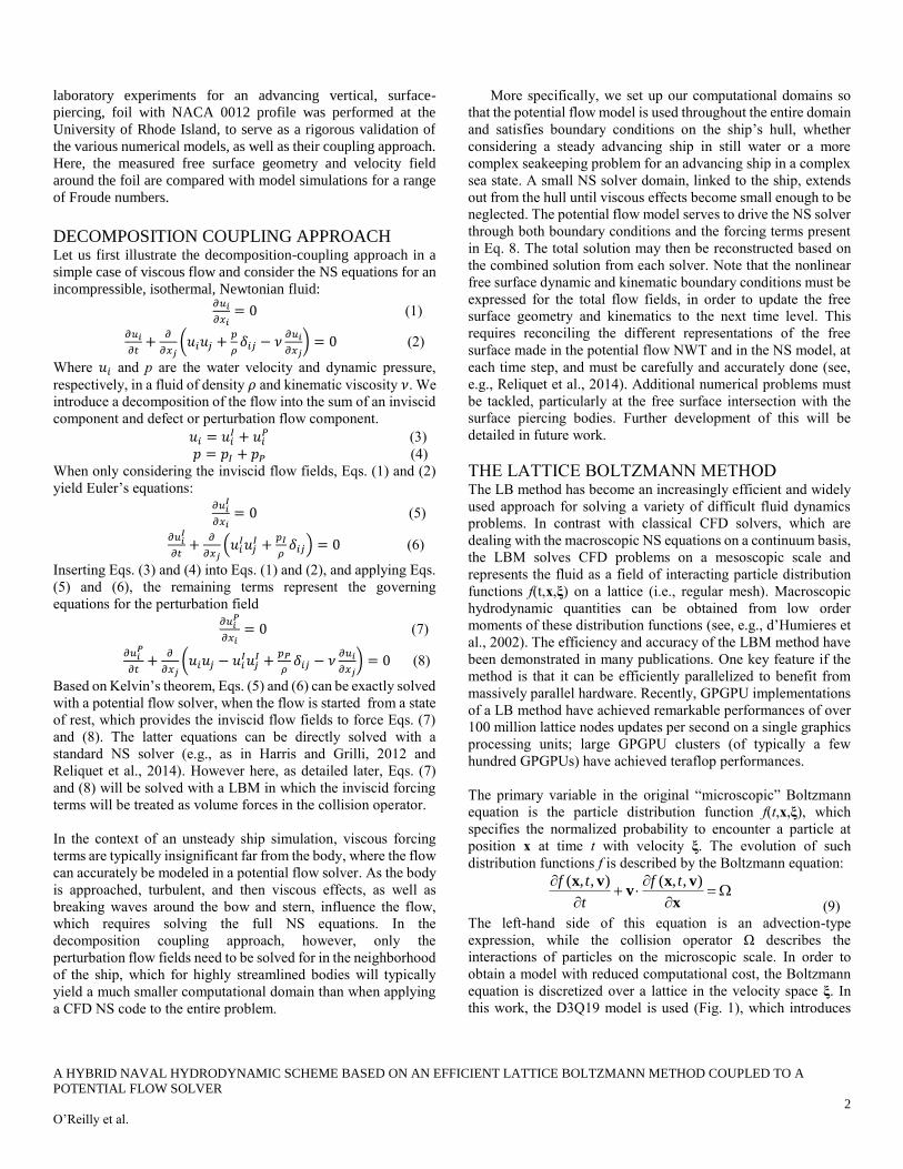
this work, the D3Q19 model is used (Fig. 1), which introduces
A HYBRID NAVAL HYDRODYNAMIC SCHEME BASED ON AN EFFICIENT LATTICE BOLTZMANN METHOD COUPLED TO A
POTENTIAL FLOW SOLVER
3
O’Reilly et al.
the following 19 discretized mesoscopic particle velocities
𝒆𝒊={0,0,0},{±c,0,0},{0,±c,0},{0,0,±c},{±c,±c,0},{±c,0,±c},
{0,±c,±c}, i = 0, . . . ,18, where the constant velocity c is related
to the speed of sound 𝑐𝑠=c/√3. The resulting set of discrete
Boltzmann equations,
i
ii
i tfe
t
tf
x
xx ),(),( (10)
have to be discretized in space and time. This is done using a
standard first-order finite difference scheme, in space and time,
on a lattice of grid spacing Δx, with c = Δx/Δt, with time step Δt.
This yields the lattice Boltzmann equation:
𝑓𝑖(𝑡 + Δ𝑡, 𝒙 + 𝑒𝑖Δ𝑡) − 𝑓𝑖(𝑡, 𝒙) = 𝛥𝑡(Ω𝑖 + 𝐹𝑖) (11)
where Fi represents effects of volume forces (e.g., here
gravitational, viscous, and inviscid forcing). Finally, Eq. (11) is
split up into a nonlinear collision step, which drives the particle
distribution functions to equilibrium locally, and a nonlocal linear
propagation step, where the post-collision particle distribution
functions are advected to the neighbor nodes in directions i as
(Fig. 1),
𝑓𝑖(𝑡, 𝒙) = 𝑓𝑖(𝑡, 𝒙) + 𝛥𝑡(Ω𝑖 + 𝐹𝑖) and
𝑓𝑖(𝑡 + Δ𝑡, 𝒙 + 𝑒𝑖Δ𝑡) = 𝑓𝑖(𝑡, 𝒙) (12)
It has been well-established that solutions of the lattice
Boltzmann equation satisfy the incompressible NS equations up
to errors of 𝑂(Δ𝑥2) and 𝑂(Ma2) (with Ma the Mach number).
Figure 1: A D3Q19 lattice scheme
The standard macroscopic values for the hydrodynamic pressure
and macroscopic fluid velocity are found from the first two
hydrodynamic moments of the particle distribution functions as,
𝑝(𝒙, 𝑡) = 𝑐𝑠2𝜌(𝒙, 𝑡) = 𝑐𝑠
2 ∑ 𝑓𝑖(𝒙, 𝑡)18𝑖=0 (13)
𝒖(𝒙, 𝑡) =1
𝜌∑ 𝒆𝑖𝑓𝑖(𝒙, 𝑡)18
𝑖=0 (14)
where denotes the fluid density. For modelling the interactions
between particles, different collision operators Ω𝑖 have been
proposed, in the context of viscous fluid flows. Here we use the
multiple relaxation time (MRT) method (d’Humieres et al.,
2002), which has been proven to be stable and accurate for high
Reynolds number flows.
Furthermore, consistent with Eq. (8), we use the LBM
perturbation coupling method first introduced in Janssen (2010),
in which additional terms are added to the MRT collision operator
to represent effects of inviscid forcing terms, which are treated as
volume forces (formally introduced in Eqs. (11) and (12) as Fi).
LBM IMPLEMENTATION We use the 3-D LBM solver elbe (developed by Dr. Janssen,
Institute for Fluid Dynamics and Ship Theory at Hamburg
University of Technology), which is based on a on equidistant
Cartesian grids. A nested mesh of increasing resolution may be
used in areas of high flow gradients and/or where more accuracy
is desired. The Smagorinsky Large Eddy Simulation (LES) model
is used to represent turbulence at the sub-grid scale. This is
implemented in the LBM model through using a turbulent (eddy)
viscosity,
𝜈𝑇 = (𝐶𝑠Δ𝑣)2||𝑺|| (15)
Where Cs represents the Sagorinsky constant and S represents a
local strain rate tensor. The details of this implementation within
the LBM context can be found in Krafczyk et al. (2003) and
Janssen et al. (2010).
In the following, we detail two methods used for free surface
representation, the Volume of Fluid (VOF) free surface interface
capturing method, which the is the standard method used in elbe
to model free surface flows, and the Level set interface tracking
method, which provides for a smoother functional representation
of the interface and has been shown to perform better in the
present context (e.g., Reliquet et al., 2014). In the future, the LS
method will be implemented in elbe.
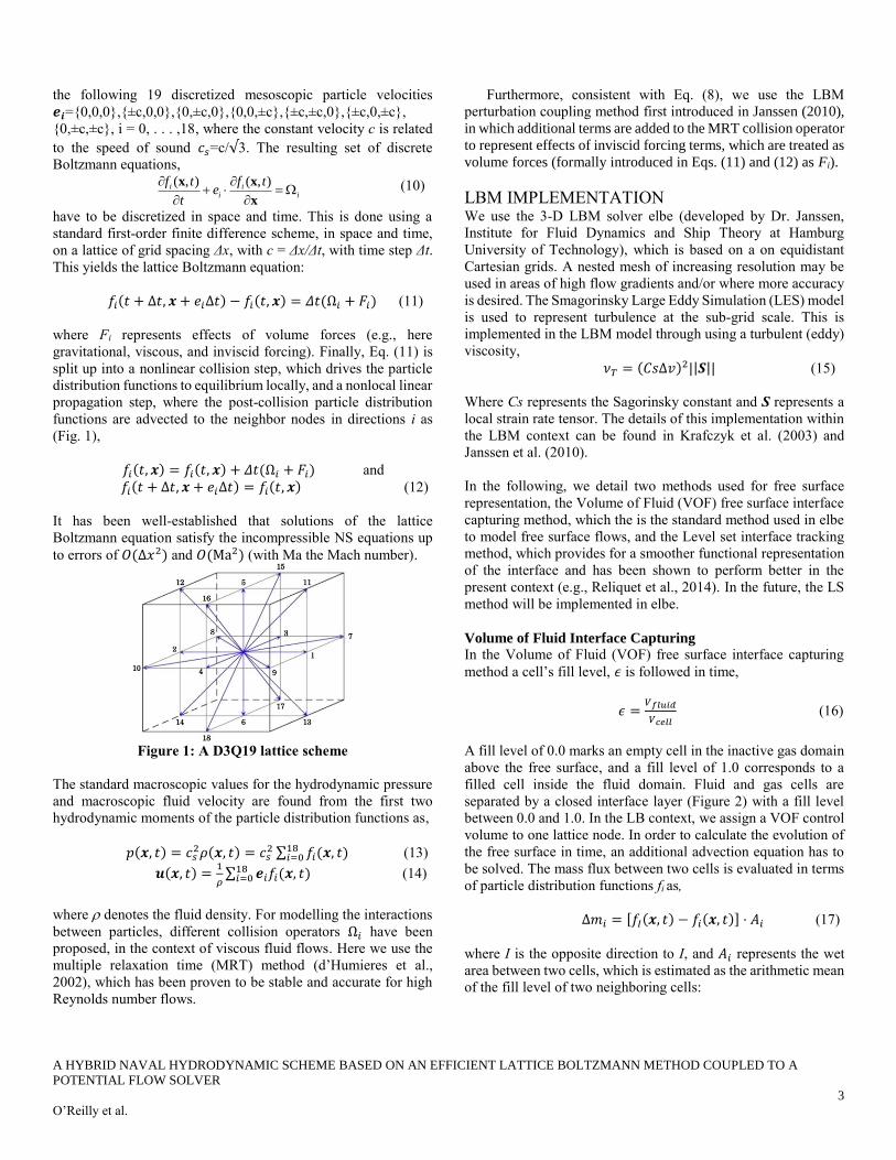
Volume of Fluid Interface Capturing
In the Volume of Fluid (VOF) free surface interface capturing
method a cell’s fill level, 𝜖 is followed in time,
𝜖 =𝑉𝑓𝑙𝑢𝑖𝑑
𝑉𝑐𝑒𝑙𝑙 (16)
A fill level of 0.0 marks an empty cell in the inactive gas domain
above the free surface, and a fill level of 1.0 corresponds to a
filled cell inside the fluid domain. Fluid and gas cells are
separated by a closed interface layer (Figure 2) with a fill level
between 0.0 and 1.0. In the LB context, we assign a VOF control
volume to one lattice node. In order to calculate the evolution of
the free surface in time, an additional advection equation has to
be solved. The mass flux between two cells is evaluated in terms
of particle distribution functions fi as,
Δ𝑚𝑖 = [𝑓𝐼(𝒙, 𝑡) − 𝑓𝑖(𝒙, 𝑡)] ⋅ 𝐴𝑖 (17)
where I is the opposite direction to I, and 𝐴𝑖 represents the wet
area between two cells, which is estimated as the arithmetic mean
of the fill level of two neighboring cells:
A HYBRID NAVAL HYDRODYNAMIC SCHEME BASED ON AN EFFICIENT LATTICE BOLTZMANN METHOD COUPLED TO A
POTENTIAL FLOW SOLVER
4
O’Reilly et al.
𝐴𝑖 = {
1.0 ∶ 𝑛𝑒𝑖𝑔ℎ𝑏𝑜𝑟 𝑓𝑙𝑢𝑖𝑑 𝑐𝑒𝑙𝑙𝜖(𝒙,𝑡)+𝜖(𝒙+𝒆𝒊,𝑡)
2∶ 𝑛𝑒𝑖𝑔ℎ𝑏𝑜𝑟 𝑖𝑛𝑡𝑒𝑟𝑓𝑎𝑐𝑒 𝑐𝑒𝑙𝑙
0.0 ∶ 𝑛𝑒𝑖𝑔ℎ𝑏𝑜𝑟 𝑔𝑎𝑠 𝑐𝑒𝑙𝑙
(18)
In contrast with higher-order schemes, the normal vector
information is not considered here. Hence, this first-order
approach in space does not conserve all line (2D) or plane (3D)
segments exactly between two time steps. Once the flux terms
have been evaluated, the new fill level of a cell can be calculated
as,
𝜖𝑛+1 =𝜌𝑛𝜖𝑛+∑ Δ𝑚𝑖𝑖
𝜌𝑛+1 (19)
Where 𝜌𝑛,𝑛+1 is the fluid density at time step n or n+1,
respectively, and the same convention applies to 𝜖. After fill
levels have been updated, several rules must be applied for
initializing new nodes and correcting 𝜖. These are detailed in
Jansen (2010).
Figure 2: Fluid (blue), interface (yellow), and gas (red) nodes
in the VOF method
Level Set Interface Tracking
In this interface tracking approach, a smooth level set (LS)
function, 𝜙 is introduced, which represents the signed distance of
a cell center to the free surface interface. The free surface is then
reconstructed as the zero-distance isosurface of the signed
distance field. However, for the interface advection, no surface
reconstruction is needed, but the motion of the surface is simply
described by the advection of the LS function as,
𝜕𝜙
𝜕𝑡+ 𝑢𝑖
𝜕𝜙
𝑥𝑖= 0 (20)
Since the LS function is smooth and continuous across the
interface, its gradient can be accurately calculated.
The LS approach is beneficial in the present hybrid method
context due to the inherent decomposition of the boundary
conditions at the free surface. Just as done above in the NS
equations, the pressure and velocity decomposition must also be
applied to the kinematic and dynamic free surface boundary
conditions, which leads to interactions between the potential flow
and LBM solvers. Therefore, neither the potential flow nor the
LBM solution will represent the correct free surface geometry
and kinematics, and one must reconstruct the correct free surface
at each time step, based on the complete solution with the
complete boundary conditions. Furthermore if the complete free
surface is above the potential flow free surface an extrapolation
will be necessary to compute the inviscid forcing fields needed in
Eq. (8). The smooth and accurate free surface representation
provided by the LS method will be important in this context.
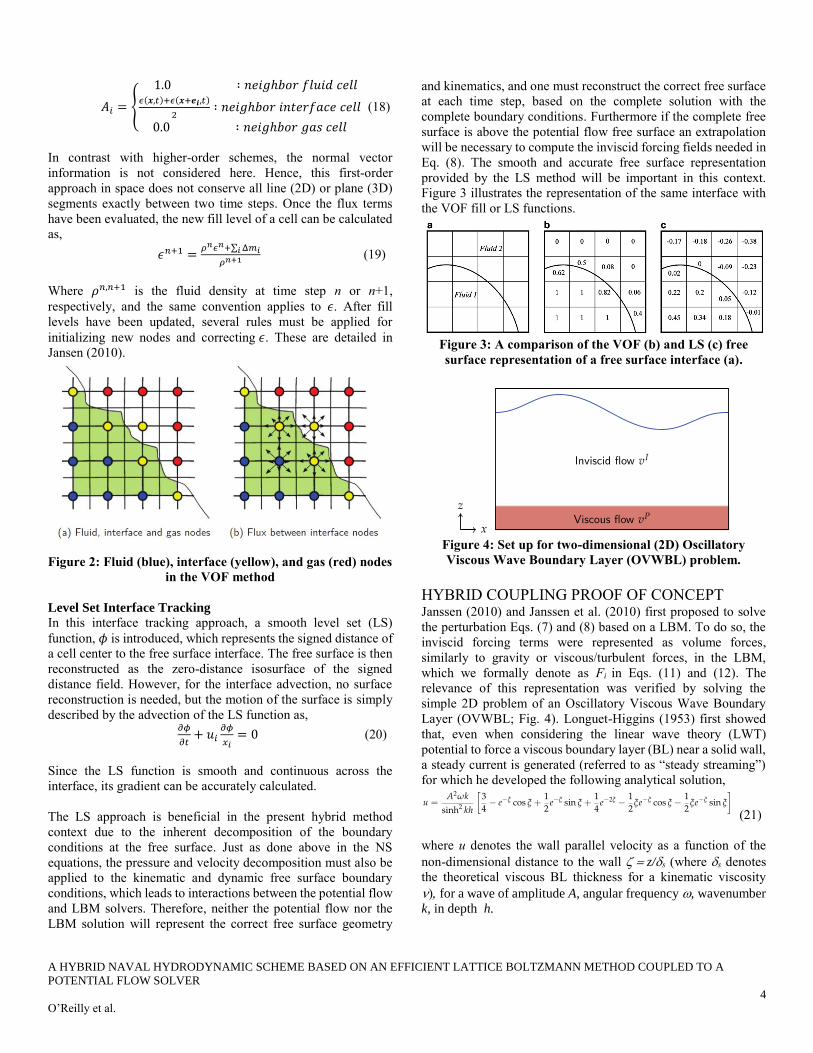
Figure 3 illustrates the representation of the same interface with
the VOF fill or LS functions.
Figure 3: A comparison of the VOF (b) and LS (c) free
surface representation of a free surface interface (a).
Figure 4: Set up for two-dimensional (2D) Oscillatory
Viscous Wave Boundary Layer (OVWBL) problem.
HYBRID COUPLING PROOF OF CONCEPT Janssen (2010) and Janssen et al. (2010) first proposed to solve
the perturbation Eqs. (7) and (8) based on a LBM. To do so, the
inviscid forcing terms were represented as volume forces,
similarly to gravity or viscous/turbulent forces, in the LBM,
which we formally denote as Fi in Eqs. (11) and (12). The
relevance of this representation was verified by solving the
simple 2D problem of an Oscillatory Viscous Wave Boundary
Layer (OVWBL; Fig. 4). Longuet-Higgins (1953) first showed
that, even when considering the linear wave theory (LWT)
potential to force a viscous boundary layer (BL) near a solid wall,
a steady current is generated (referred to as “steady streaming”)
for which he developed the following analytical solution,
(21)
where u denotes the wall parallel velocity as a function of the
non-dimensional distance to the wall z/s (where s denotes
the theoretical viscous BL thickness for a kinematic viscosity
)for a wave of amplitude A, angular frequency , wavenumber
k, in depth h.
A HYBRID NAVAL HYDRODYNAMIC SCHEME BASED ON AN EFFICIENT LATTICE BOLTZMANN METHOD COUPLED TO A
POTENTIAL FLOW SOLVER
5
O’Reilly et al.
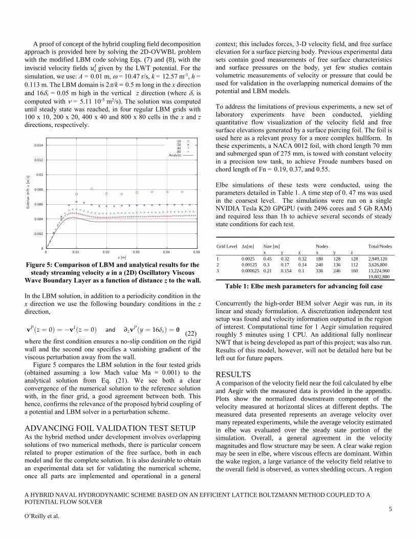
A proof of concept of the hybrid coupling field decomposition
approach is provided here by solving the 2D-OVWBL problem
with the modified LBM code solving Eqs. (7) and (8), with the
inviscid velocity fields 𝑢𝑖𝐼 given by the LWT potential. For the
simulation, we use: A = 0.01 m, = 10.47 r/s, k = 12.57 m-1, h =
0.113 m. The LBM domain is 2/k = 0.5 m long in the x direction
and 16s = 0.05 m high in the vertical z direction (where s is
computed with = 5.11 10-5 m2/s). The solution was computed
until steady state was reached, in four regular LBM grids with
100 x 10, 200 x 20, 400 x 40 and 800 x 80 cells in the x and z
directions, respectively.
Figure 5: Comparison of LBM and analytical results for the
steady streaming velocity u in a (2D) Oscillatory Viscous
Wave Boundary Layer as a function of distance z to the wall.
In the LBM solution, in addition to a periodicity condition in the
x direction we use the following boundary conditions in the z
direction,
(22)
where the first condition ensures a no-slip condition on the rigid
wall and the second one specifies a vanishing gradient of the
viscous perturbation away from the wall.
Figure 5 compares the LBM solution in the four tested grids
(obtained assuming a low Mach value Ma = 0.001) to the
analytical solution from Eq. (21). We see both a clear
convergence of the numerical solution to the reference solution
with, in the finer grid, a good agreement between both. This
hence, confirms the relevance of the proposed hybrid coupling of
a potential and LBM solver in a perturbation scheme.
ADVANCING FOIL VALIDATION TEST SETUP As the hybrid method under development involves overlapping
solutions of two numerical methods, there is particular concern
related to proper estimation of the free surface, both in each
model and for the complete solution. It is also desirable to obtain
an experimental data set for validating the numerical scheme,
once all parts are implemented and operational in a general
context; this includes forces, 3-D velocity field, and free surface
elevation for a surface piercing body. Previous experimental data
sets contain good measurements of free surface characteristics
and surface pressures on the body, yet few studies contain
volumetric measurements of velocity or pressure that could be
used for validation in the overlapping numerical domains of the
potential and LBM models.
To address the limitations of previous experiments, a new set of
laboratory experiments have been conducted, yielding
quantitative flow visualization of the velocity field and free
surface elevations generated by a surface piercing foil. The foil is
used here as a relevant proxy for a more complex hullform. In
these experiments, a NACA 0012 foil, with chord length 70 mm
and submerged span of 275 mm, is towed with constant velocity
in a precision tow tank, to achieve Froude numbers based on
chord length of Fn = 0.19, 0.37, and 0.55.
Elbe simulations of these tests were conducted, using the
parameters detailed in Table 1. A time step of 0. 47 ms was used
in the coarsest level. The simulations were run on a single
NVIDIA Tesla K20 GPGPU (with 2496 cores and 5 Gb RAM)
and required less than 1h to achieve several seconds of steady
state conditions for each test.
Table 1: Elbe mesh parameters for advancing foil case
Concurrently the high-order BEM solver Aegir was run, in its
linear and steady formulation. A discretization independent test
setup was found and velocity information outputted in the region
of interest. Computational time for 1 Aegir simulation required
roughly 5 minutes using 1 CPU. An additional fully nonlinear
NWT that is being developed as part of this project; was also run.
Results of this model, however, will not be detailed here but be
left out for future papers.
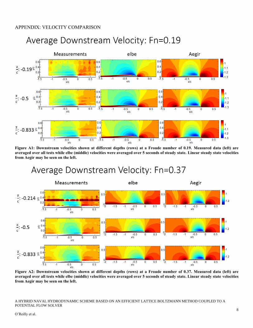
RESULTS A comparison of the velocity field near the foil calculated by elbe
and Aegir with the measured data is provided in the appendix.
Plots show the normalized downstream component of the
velocity measured at horizontal slices at different depths. The
measured data presented represents an average velocity over
many repeated experiments, while the average velocity estimated
in elbe was evaluated over the steady state portion of the
simulation. Overall, a general agreement in the velocity
magnitudes and flow structure may be seen. A clear wake region
may be seen in elbe, where viscous effects are dominant. Within
the wake region, a large variance of the velocity field relative to
the overall field is observed, as vortex shedding occurs. A region
Grid Level Δx[m] Size [m] Nodes
Total/Nodes
x y z x y z
1 0.0025 0.45 0.32 0.32 180 128 128 2,949,120
2 0.00125 0.3 0.17 0.14 240 136 112 3,626,800
3 0.000625 0.21 0.154 0.1 336 246 160 13,224,960
19,802,880
A HYBRID NAVAL HYDRODYNAMIC SCHEME BASED ON AN EFFICIENT LATTICE BOLTZMANN METHOD COUPLED TO A
POTENTIAL FLOW SOLVER
6
O’Reilly et al.
of less accurate experimental data may be observed in the
shallowest slice (Fn=0.37), which is likely the result of
insufficient particle seeding within the region, during
measurements. A larger interrogation window within this region
is likely necessary to properly evaluate velocities within the
region. As velocity increases, the free surface’s influence
becomes more prevalent within the velocity field, resulting from
the formation of wakes of larger amplitude and wavelength.
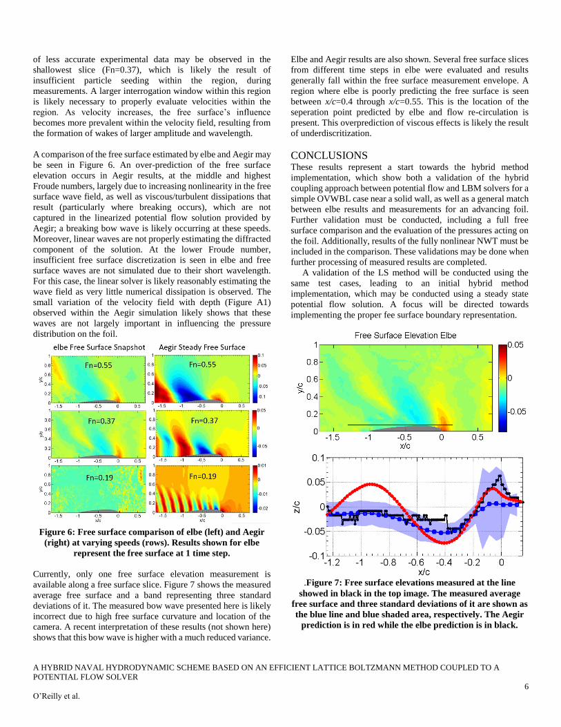
A comparison of the free surface estimated by elbe and Aegir may
be seen in Figure 6. An over-prediction of the free surface
elevation occurs in Aegir results, at the middle and highest
Froude numbers, largely due to increasing nonlinearity in the free
surface wave field, as well as viscous/turbulent dissipations that
result (particularly where breaking occurs), which are not
captured in the linearized potential flow solution provided by
Aegir; a breaking bow wave is likely occurring at these speeds.
Moreover, linear waves are not properly estimating the diffracted
component of the solution. At the lower Froude number,
insufficient free surface discretization is seen in elbe and free
surface waves are not simulated due to their short wavelength.
For this case, the linear solver is likely reasonably estimating the
wave field as very little numerical dissipation is observed. The
small variation of the velocity field with depth (Figure A1)
observed within the Aegir simulation likely shows that these
waves are not largely important in influencing the pressure
distribution on the foil.
Figure 6: Free surface comparison of elbe (left) and Aegir
(right) at varying speeds (rows). Results shown for elbe
represent the free surface at 1 time step.
Currently, only one free surface elevation measurement is
available along a free surface slice. Figure 7 shows the measured
average free surface and a band representing three standard
deviations of it. The measured bow wave presented here is likely
incorrect due to high free surface curvature and location of the
camera. A recent interpretation of these results (not shown here)
shows that this bow wave is higher with a much reduced variance.
Elbe and Aegir results are also shown. Several free surface slices
from different time steps in elbe were evaluated and results
generally fall within the free surface measurement envelope. A
region where elbe is poorly predicting the free surface is seen
between x/c=0.4 through x/c=0.55. This is the location of the
seperation point predicted by elbe and flow re-circulation is
present. This overprediction of viscous effects is likely the result
of underdiscritization.
CONCLUSIONS
These results represent a start towards the hybrid method
implementation, which show both a validation of the hybrid
coupling approach between potential flow and LBM solvers for a
simple OVWBL case near a solid wall, as well as a general match
between elbe results and measurements for an advancing foil.
Further validation must be conducted, including a full free
surface comparison and the evaluation of the pressures acting on
the foil. Additionally, results of the fully nonlinear NWT must be
included in the comparison. These validations may be done when
further processing of measured results are completed.
A validation of the LS method will be conducted using the
same test cases, leading to an initial hybrid method
implementation, which may be conducted using a steady state
potential flow solution. A focus will be directed towards
implementing the proper fee surface boundary representation.
.Figure 7: Free surface elevations measured at the line
showed in black in the top image. The measured average
free surface and three standard deviations of it are shown as
the blue line and blue shaded area, respectively. The Aegir
prediction is in red while the elbe prediction is in black.
A HYBRID NAVAL HYDRODYNAMIC SCHEME BASED ON AN EFFICIENT LATTICE BOLTZMANN METHOD COUPLED TO A
POTENTIAL FLOW SOLVER
7
O’Reilly et al.
ACKNOWLEDGEMENTS
This work was supported by the Office of Naval Research, PM
Kelly Cooper. The authors gratefully acknowledge this support.
REFERENCES
Banari A., Janssen C.F., and Grilli S.T. 2014. An efficient
lattice Boltzmann multiphase model for 3D flows with large
density ratios at high Reynolds numbers. Comp. Math. with Appl.,
68, 1819-1843, doi:10.1016/j.camwa.2014.10.009 .
Grilli, S.T., Dias, F., Guyenne, P., Fochesato, C. and F. Enet
2010. Progress In Fully Nonlinear Potential Flow Modeling Of
3D Extreme Ocean Waves. Chapter 3 in Advances in Numerical
Simulation of Nonlinear Water Waves (ISBN: 978-981-283-649-
6, edited by Q.W. Ma) (Vol. 11 in Series in Advances in Coastal
and Ocean Engineering). World Scientific Publishing Co. Pte.
Ltd., pps. 75- 128.
Harris, J.C. and S.T. Grilli 2012. A perturbation approach to
large-eddy simulation of wave-induced bottom boundary layer
flows. Intl. J. Numer. Meth. Fluids, 68, 1,574-1,604,
doi:10.1002/fld.2553
Harris, J.C., Dombre, E., Benoit, M. and S.T. Grilli 2014. Fast
integral equation methods for fully nonlinear water wave
modeling. In Proc. 24th Offshore and Polar Engng. Conf.
(ISOPE14, Busan, South Korea, June 2014), Intl. Society of
Offshore and Polar Engng., pps. 583-590.
d’Humieres D., T. Ginzburg, M. Krafczyk, P. Lallemand, and
L.-S. Luo 2002. Multiple Relaxation-Time Lattice Boltzmann
models in three-dimensions. Royal Soc. Lond. Phil. Trans., A360,
437–451.
Janssen C.F., S.T. Grilli and M. Krafczyk 2010. Modeling of
Wave Breaking and Wave-Structure Interactions by Coupling of
Fully Nonlinear Potential Flow and Lattice-Boltzmann Models.
In Proc. 20th Offshore and Polar Engng. Conf. (ISOPE10,
Beijing, China, June 20-25, 2010), pps. 686-693. Intl. Society of
Offshore and Polar Engng.
Janssen, C.F. 2010. Kinetic approaches for the simulation of
non-linear free surface flow problems in civil and environmental
engineering. PhD thesis, Technical University Braunschweig.
Janssen, C.F., S.T. Grilli and M. Krafczyk 2013. On enhanced
non-linear free surface flow simulations with a hybrid LBM-VOF
approach. Computers and Mathematics with Applications, 65(2),
211-229, doi:10.1016/j.camwa.2012.05.012 (published online
7/12/12).
Krafczyk, M., Tölke, J., and Luo, L.-S. 2003. Large eddy
simulations with a multiple-relaxation-time LBE model. Int. J.
Mod. Phys. B, 17, 33–39.
Longuet-Higgins, M.S. 1953. Mass transport in water waves.
Phil. Trans. Royal Soc. London, A, 535–581.
Reliquet, G., A. Drouet, P.-E. Guillerm, L. Gentaz and P.
Ferrant 2014. Simulation of wave-ship interaction in regular and
irregular seas under viscous flow theory using the SWENSE
method. In Proc. 30th Symposium on Naval Hydrodynamics
(Hobart, Tasmania, Australia, 2-7 November, 2014), 11 pps.
A HYBRID NAVAL HYDRODYNAMIC SCHEME BASED ON AN EFFICIENT LATTICE BOLTZMANN METHOD COUPLED TO A
POTENTIAL FLOW SOLVER
8
O’Reilly et al.
APPENDIX: VELOCITY COMPARISON
Figure A1: Downstream velocities shown at different depths (rows) at a Froude number of 0.19. Measured data (left) are
averaged over all tests while elbe (middle) velocities were averaged over 5 seconds of steady state. Linear steady state velocities
from Aegir may be seen on the left.
Figure A2: Downstream velocities shown at different depths (rows) at a Froude number of 0.37. Measured data (left) are
averaged over all tests while elbe (middle) velocities were averaged over 5 seconds of steady state. Linear steady state velocities
from Aegir may be seen on the left.
A HYBRID NAVAL HYDRODYNAMIC SCHEME BASED ON AN EFFICIENT LATTICE BOLTZMANN METHOD COUPLED TO A
POTENTIAL FLOW SOLVER
9
O’Reilly et al.
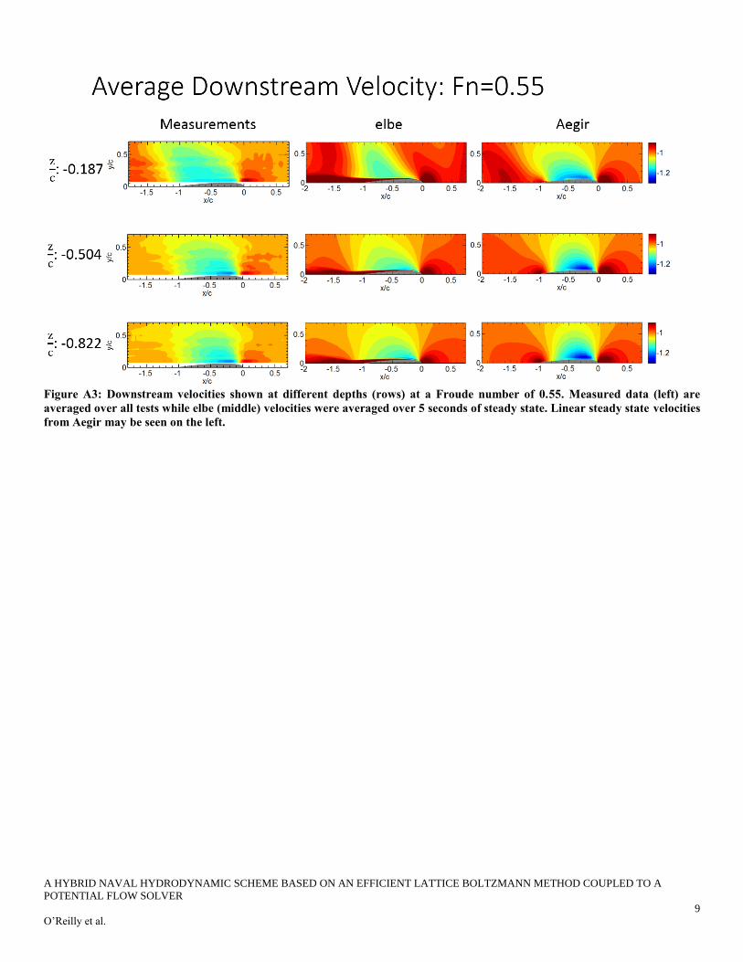
Figure A3: Downstream velocities shown at different depths (rows) at a Froude number of 0.55. Measured data (left) are
averaged over all tests while elbe (middle) velocities were averaged over 5 seconds of steady state. Linear steady state velocities
from Aegir may be seen on the left.