BIONAVIGATION: SELECTING RESOURCES TO EVALUATE SCIENTIFIC

QUERIES

by

Kaushal D. Parekh

A Internship Report Presented in Partial Fulfillmentof the Requirements for the Degree

MASTER OF SCIENCE

ARIZONA STATE UNIVERSITY

August 2005

ABSTRACT

Advances in genome science have created a surge of data. These data critical to sci-

entific discovery are made available in thousands of heterogeneous public resources. Each

of these resources provides biological data with a specific data organization, format, and

quality, object identification, and a variety of capabilities that allow scientists to access, an-

alyze, cluster, visualize and navigate through the datasets. The heterogeneity of biological

resources and their increasing number make it difficult for scientists to exploit and under-

stand them. Learning the properties of a new resource is a tedious and time-consuming

process, often made more difficult by the many changes made on the resources (new or

changed information, capabilities) that stress scientists keeping their knowledge up-to-date.

Therefore many scientists master a few resources while ignoring others that may provide

additional data and useful capabilities. The BioNavigation system completes existing data

integration approaches, by allowing users to explore biological resources. The BioNaviga-

tion system provides the scientist with valuable guidance in selecting the most effective

evaluation path through the physical resources for his ontological query. It allows the user

to visualize the conceptual level ontology, the physical graph of resources and the map-

pings between the two levels and browse the graphs to obtain more information about the

resources; build queries with the help of the ontology by selecting the desired classes con-

nected by labeled relationships; and obtain all possible physical paths that implement the

query and rank them to optimize certain user selected criteria. BioNavigation could also be

coupled with a data integration tool that would allow users to collect data automatically

after selecting the resources.

ii

ACKNOWLEDGMENTS

This work was partially supported by the National Science Foundation, Divi-

sion of Computer and Information Science and Engineering, through the grant IIS-

0223042(September 2003 - August 2005).

The Project has also benefited from valuable inputs from Peter Schwarz and Julia

Rice at the IBM Almaden Research Center and Barbara Eckman at IBM Life Sciences.

Michael Berens, Anna Joy and scientists at the Neurogenomics Division of the Trans-

lational Genomics Research Institute (TGen), Phoenix, provided support in determining the

requirements of the system and helping test the prototype.

Students at the Scientific Data Management Lab, Herve Menager and Pallavi

Mudumby provided valuable feedback and comments.

Finally and most importantly, I would like to thank my internship advisor, Dr. Zoe

Lacroix, for providing me with the opportunity to work as a Research Assistant at the

Scientific Data Management Lab and present our work at several prestigious conferences.

iii

TABLE OF CONTENTS

Page

LIST OF FIGURES . . . . . . . . . . . . . . . . . . . . . . . . . . . . . . . . . . . . vi

CHAPTER 1 Introduction and Motivation . . . . . . . . . . . . . . . . . . . . . . . 1

1. Complexity in Biological Resources . . . . . . . . . . . . . . . . . . . . . . . 1

2. Problems in Scientific Data Collection . . . . . . . . . . . . . . . . . . . . . 3

3. Existing Integration Systems . . . . . . . . . . . . . . . . . . . . . . . . . . 4

4. The BioNavigation Approach . . . . . . . . . . . . . . . . . . . . . . . . . . 6

CHAPTER 2 Graph Representation of Resources . . . . . . . . . . . . . . . . . . . 8

1. Bi-Level Representation . . . . . . . . . . . . . . . . . . . . . . . . . . . . . 8

1.1. The Physical Graph . . . . . . . . . . . . . . . . . . . . . . . . . . . 10

1.2. The Logical or Conceptual Graph . . . . . . . . . . . . . . . . . . . 11

2. The BioMetaDatabase . . . . . . . . . . . . . . . . . . . . . . . . . . . . . . 12

2.1. Metadata for Data Sources . . . . . . . . . . . . . . . . . . . . . . . 13

2.2. Metadata for capabilities . . . . . . . . . . . . . . . . . . . . . . . . 14

CHAPTER 3 Use of Ontology for Data Integration . . . . . . . . . . . . . . . . . . 16

1. What is Ontology? . . . . . . . . . . . . . . . . . . . . . . . . . . . . . . . . 16

1.1. Applications . . . . . . . . . . . . . . . . . . . . . . . . . . . . . . . 18

2. Need for Ontologies in Biological Data Management . . . . . . . . . . . . . 19

3. OWL: The Web Ontology Language . . . . . . . . . . . . . . . . . . . . . . 22

4. Protege Ontology Editor . . . . . . . . . . . . . . . . . . . . . . . . . . . . . 22

5. The BioNavigation Ontology . . . . . . . . . . . . . . . . . . . . . . . . . . 23

iv

Page

CHAPTER 4 Querying Integrated Biology Data Sources - Esearch Algorithm . . . 25

1. Query Language . . . . . . . . . . . . . . . . . . . . . . . . . . . . . . . . . 25

2. ESearch Algorithm . . . . . . . . . . . . . . . . . . . . . . . . . . . . . . . . 27

3. Ranking Criteria . . . . . . . . . . . . . . . . . . . . . . . . . . . . . . . . . 28

CHAPTER 5 The BioNavigation Interface . . . . . . . . . . . . . . . . . . . . . . . 30

1. Interface Requirements . . . . . . . . . . . . . . . . . . . . . . . . . . . . . . 30

1.1. Browsing . . . . . . . . . . . . . . . . . . . . . . . . . . . . . . . . . 31

1.2. Querying . . . . . . . . . . . . . . . . . . . . . . . . . . . . . . . . . 32

1.3. Interpreting Results . . . . . . . . . . . . . . . . . . . . . . . . . . . 33

2. Using the BioNavigation System . . . . . . . . . . . . . . . . . . . . . . . . 34

CHAPTER 6 Future Work and Conclusions . . . . . . . . . . . . . . . . . . . . . . 41

REFERENCES . . . . . . . . . . . . . . . . . . . . . . . . . . . . . . . . . . . . . . . 43

v

LIST OF FIGURES

Figure Page

1. Mapping physical resources to the conceptual level . . . . . . . . . . . . . . 9

2. An Example Ontology of Concepts and Associations . . . . . . . . . . . . . 24

3. BNF grammar of regular expressions . . . . . . . . . . . . . . . . . . . . . . 27

4. The BioNavigation Interface . . . . . . . . . . . . . . . . . . . . . . . . . . . 35

5. Genecards Properties Window . . . . . . . . . . . . . . . . . . . . . . . . . . 36

6. Properties Window for the OMIM to CGAP Link . . . . . . . . . . . . . . . 37

7. Output for the ‘disease-protein’ Query . . . . . . . . . . . . . . . . . . . . . 38

8. Disease to Citation with 3 Intermediate Nodes . . . . . . . . . . . . . . . . 39

9. Disease to Protein with one Intermediate Node . . . . . . . . . . . . . . . . 39

10. Using any number of Intermediate Nodes . . . . . . . . . . . . . . . . . . . 40

11. Gene-Citation query with 0 or more intermediates 2 output s for target object

and path cardinality ranking . . . . . . . . . . . . . . . . . . . . . . . . . . 40

vi

CHAPTER 1

Introduction and Motivation

A scientific data collection protocol is always specified in terms of scientific classes

being studied and it need not specify the data sources from which to get the information

about these classes. These protocols are also mostly navigational, i.e. scientists start with

obtaining information about a particular scientific object then from there go to another

using the provided links and so on, thus forming a path. Scientists tend to use only a set of

resources which they are familiar with to express their protocols rather than selecting the

best possible resource that matches their needs. Most of the times, they do not even know

which is the best resource, or even if they are aware that such a source exists, they are not

familiar with its features and query interface to effectively exploit it.

1. Complexity in Biological Resources

With new advances in the biological sciences, the number of available data sources

is increasing dramatically. The key to scientific discovery lies in effectively exploiting the

wealth of publicly available data, but this is not simple. For example, the current number of

public molecular biology databases according to the 2005 update [Galp 05] in the Database

issue of Nucleic Acids Research, is 719 databases compared to 548 in 2004 and 386 in year

2

2003. Not only is the number of sources large and increasing, but the data repositories

themselves are highly heterogeneous. They organize biological data differently, they struc-

ture their data in multiple ways (even two resources with the same overall organization use

different schemas) and publish them in various formats (flat files, relational tables, XML,

etc.). Also, it is not unnatural that there exists an overlap of data in multiple resources.

Each resource offers a different level of curation that affects data quality. In addition, re-

sources are not always up-to-date; some sources may have more recent information than

others.

Each data source offers to the users a set of capabilities that help to access, navigate,

visualize, and perform other operations on the datasets. These capabilities are also highly

heterogeneous among different databases. for example, GeneCards [Rebh 97] allows users

to search for genes through a single full text search, while Genew [Gene 05] allows searching

of genes with additional specifications such as approved symbol, approved gene name, etc.

Other sources provide analytic (e.g. NCBI BLAST1) or navigational (e.g. PubMed2 links

from OMIM3 records) capabilities.

It is difficult to stay at par with the characteristics of each source and its capabilities,

and as a consequence, scientists tend to limit themselves to a few that they are familiar

with. They would rather spend their valuable time on research than learning how to access

a new data source; and as a price, miss out on information that could significantly affect

their research. The public resources evolve significantly over time which adds to the above

complexity. Although these changes allow the data sources to keep up with new data and

improve the support provided to scientists, they contribute to the increasing burden of

1NCBI BLAST - http://www.ncbi.nlm.nih.gov/BLAST/2PubMed Literature Database - http://www.ncbi.nlm.nih.gov/entrez/query.fcgi?DB=pubmed3Online Mendelian Inheritance in Man - http://www.ncbi.nlm.nih.gov/entrez/query.fcgi?db=OMIM

3

mastering the biological resources.

2. Problems in Scientific Data Collection

Exploiting the complex maze of publicly available Biological resources to implement

scientific data collection pipelines poses a multitude of challenges to biologists. Their first

challenge is to accurately reflect the scientific question at hand in expressing the query.

Ideally the scientists should not deal with the properties of the data sources intended to

be used while framing this query. The query should be constructed only in terms of the

higher level scientific concepts involved while keeping the implementation details transpar-

ent. Instead, scientists build their queries to adapt to the characteristics and limitations of

the resources that they are familiar with.

Another challenge lies in the availability of multiple resources serving similar pur-

poses. For example, you can get information about a particular ‘gene’ (Which is a higher

level scientific concept) from various alternate data sources like NCBI Gene4 or GeneCards5

or OMIM etc. These resources, although they all provide information about genes, are

highly heterogeneous with respect to the data format, number of records, level of curation,

navigational capabilities or links to other resources, etc. Thus, when the query involves

multiple scientific concepts, the same higher level query can be translated to various evalu-

ation paths involving a number of different alternate data sources, links, and applications.

Each of these paths might have different semantic meanings and is bound to provide to the

scientist with a different set of results [Lacr 04a]. Hence, it becomes important for the user

to understand what path is best suited to his purpose to get the best possible set of results

from the query.

4NCBI Gene Database - http://www.ncbi.nlm.nih.gov/entrez/query.fcgi?db=gene5GeneCards gene database - http://www.genecards.org/

4

Once the scientist has decided what resources he will use to evaluate his query, then

the challenge lies in effectively formulating the query in the format acceptable to those

resources and collecting and utilizing the data. All resources have different query interfaces

and we can not expect the biologist to be always up to date with the query language, data

format of all of them. This problem is usually taken care of by many available integrated

database systems and hence we do not deal with this issue. Examples of such systems are

described in the next section.

3. Existing Integration Systems

There are a few systems that address the need of integrated access to multiple data

sources; examples of which are DB2 Information Integrator [Haas 03], TAMBIS [Bake 98],

and SRS [Etzo 03]. The characteristics of these systems are briefly described below.

• The DB2 Information Integrator system (Now known as WebSphere Information In-

tegrator, and previously known as Discovery Link) allows the integration of non-

relational data sources (flat file, XML, Web resources) and other relational databases

with the DB2 relational database so that they can be queried through a single DB2

query interface. This is done with the help of wrappers that encapsulate query and

search capabilities of the resources into user-defined functions. In simplified terms,

the wrapper translates the relational query (written in SQL) into resource specific set

of queries or web requests. The data retrieved from these is then converted into a

relational (tabular) form according to the predefined schema for that wrapper. The

system comes with certain built in wrappers for popular bioinformatics resources such

as Entrez, Blast, etc. and also provides toolkits for C and Java languages to develop

custom wrappers for additional resources.

5

• The TAMBIS (Transparent Access to Multiple Bioinformatics Information Sources)

system acts as a virtual integrated data source by providing transparent information

retrieval from various wrapped data sources with the help of a mediator. The medi-

ator uses an ontology to describe a conceptual model of the data sources and assists

the users in expressing queries against this universal model. The user can thus write

queries in terms of the universal model or ontology while remaining unaware of what

resources will be used to implement it. The mediator then translates these concep-

tual queries to corresponding mapped source queries which are sent to the individual

wrappers for the sources. These wrappers then send the actual queries or calls to each

respective resource, retrieve the data and reformat in accordance with the conceptual

model so that results from different heterogeneous resources are presented in the same

format.

• The SRS (Sequence Retrieval System) provides a single interface to access a large

number of bioinformatics data sources and tools which can be queried in the same

way regardless of the heterogeneous formats through a simple graphical interface. In

the same manner, the results of the analysis can also be viewed through a single

interface and are presented in a uniform format. SRS also allows users to exploit the

links between various resources allowing for queries that can take the user from one

data source to another and thus are navigational in nature.

The problem with the above and also most other available systems is that they either

expect the user to specify explicitly the resources involved in the data collection process

(e.g., DB2 and SRS), or the system transparently chooses a particular database for the user

(e.g. TAMBIS). There are obviously critical issues with both the approaches that may affect

the data collection process, and thus the quality and completeness of the retrieved data. As

6

explained previously, we can not expect the user to know all available resources and choose

the most appropriate one to exploit. On the other hand the transparent access does not

allow the user to play an important role in the selection of the particular data sources and

capabilities, so while the scientist is able to avoid this tedious task, the provenance of the

data collected is hidden from the user.

4. The BioNavigation Approach

To summarize the problems discussed above:

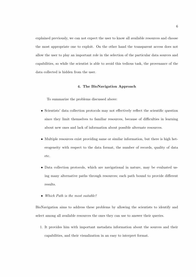
• Scientists’ data collection protocols may not effectively reflect the scientific question

since they limit themselves to familiar resources, because of difficulties in learning

about new ones and lack of information about possible alternate resources.

• Multiple resources exist providing same or similar information, but there is high het-

erogeneity with respect to the data format, the number of records, quality of data

etc.

• Data collection protocols, which are navigational in nature, may be evaluated us-

ing many alternative paths through resources; each path bound to provide different

results.

• Which Path is the most suitable?

BioNavigation aims to address these problems by allowing the scientists to identify and

select among all available resources the ones they can use to answer their queries.

1. It provides him with important metadata information about the sources and their

capabilities, and their visualization in an easy to interpret format.

7

2. It also assists scientists in looking at their protocols at the higher conceptual level and

building the corresponding queries graphically.

3. BioNavigation then presents the user with various possible implementations of their

query so that the user can choose the best one that suits his purposes.

4. The user then just has to use one his favorite tools (web interfaces, Perl scripts or any

mediation system described above), but this time with the confidence that all possible

resources were exploited, to get the data.

BioNavigation could also be used as an interface to employ a mediation or integration

system such as the ones described above to evaluate the particular implementation path

that the user selected. The remainder of this Internship report describes the various aspects

of the design and development of this BioNavigation system.

CHAPTER 2

Graph Representation of Resources

Scientists should be able to formulate their queries at the higher conceptual level

of scientific classes and their relationships, without the concern of what source would be

used underneath to collect the data. This is the ontology level. Classes in the ontology are

mapped to the data sources which represent them, for e.g. the scientific class ’gene’ is repre-

sented by many sources such as Entrez Gene, GeneCards, etc. Similarly the relationships in

the ontology are mapped to the physical links between the data sources. These links could

be in the form of navigational links, indices or applications that capture the semantics of

the ontology level relationships.

1. Bi-Level Representation

Most data sources typically represent a particular type of scientific class. For ex-

ample, PubMed provides references to published literature, UniProt1 provides information

about proteins, etc. There can be several data sources for the same scientific class. For

example, one can retrieve ’DNA sequences’ from either NCBI Nucleotide2 or EMBL3.

1UniProt - http://www.ebi.ac.uk/uniprot/2NCBI Nucleotide - http://www.ncbi.nlm.nih.gov/entrez/query.fcgi?db=nucleotide3EMBL - http://www.ebi.ac.uk/embl/

9

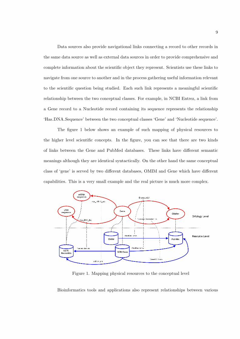
Data sources also provide navigational links connecting a record to other records in

the same data source as well as external data sources in order to provide comprehensive and

complete information about the scientific object they represent. Scientists use these links to

navigate from one source to another and in the process gathering useful information relevant

to the scientific question being studied. Each such link represents a meaningful scientific

relationship between the two conceptual classes. For example, in NCBI Entrez, a link from

a Gene record to a Nucleotide record containing its sequence represents the relationship

‘Has DNA Sequence’ between the two conceptual classes ‘Gene’ and ‘Nucleotide sequence’.

The figure 1 below shows an example of such mapping of physical resources to

the higher level scientific concepts. In the figure, you can see that there are two kinds

of links between the Gene and PubMed databases. These links have different semantic

meanings although they are identical syntactically. On the other hand the same conceptual

class of ‘gene’ is served by two different databases, OMIM and Gene which have different

capabilities. This is a very small example and the real picture is much more complex.

Figure 1. Mapping physical resources to the conceptual level

Bioinformatics tools and applications also represent relationships between various

10

scientific classes represented by the inputs and outputs of the application. Consider the

example of a BLAST search for finding similar nucleotide sequences. in simplified terms,

the input and output belong to the scientific class ‘Nucleotide sequence’ and the tool itself

implements the relationship ‘Has Similar Sequence’ between two nucleotide sequences.

As described in the previous chapter, a scientific data collection protocol is ideally

designed at the conceptual level, whereas the implementation is at the physical level of the

resources. Thus it becomes important to define formally the two levels of representation

which will be used by the BioNavigation system.

1.1. The Physical Graph. The physical graph represents the resource level. In

the first version of the BioNavigation system[Lacr 04b] and the ESearch algorithm[Lacr 04d,

Lacr 04c], the physical graph consisted of data sources and the links between them as nodes

and edges of the graph respectively. A navigational query would then be represented as a

sequence of data sources. There are two major limitations to this model for the resource

level.

1. There can be more than one type of links between two particular sources with different

semantics. For example, in Figure 1, consider the links to PubMed citations from the

NCBI Gene database. There are two types of links ‘PubMed Links’ and ‘GeneRIF

Links’, which are the same at the physical level since they are links from a Gene

record to a PubMed record. But they have different meanings; the first set of links

consists of citations that are related to the gene in general whereas the other set of

links represents citations that specifically provide a functional annotation for the gene.

The representation of links as simple edges in a graph does not allow for capturing

these differences in multiple edges between the same set of nodes.

11

2. The graph representation in the first version of BioNavigation also does not include

the tools and applications which are often part of a data collection protocol. Although

applications may represent a scientific relationship between two classes, they are dif-

ferent from links in that they are not bound to a specific data source, but always can

be plugged in between two data sources which match the input and output class types

of the application respectively.

Taking the above limitations into consideration we defined the new graph model

[Lacr 05b] for the physical level where all the resources, i.e., data sources, links and appli-

cations are modeled as different types of nodes. The edges in the graph are used only to

specify the direction of association. The Physical Graph PG = (VP , L) is a directed graph,

where:

• VP is a set of nodes, partitioned into three subsets, S, AP , and QC, such that,

S represents physical data sources, AP represents applications, and QC represents

query capabilities.

• L is a set of directed edges L ⊆ VP × VP that represents the directional associations

between sources and applications or query capabilities. If a pair (a, b) belongs to L

then, a is a source and b is an application or query capability, or a is an application

or query capability and b is a source.

1.2. The Logical or Conceptual Graph. The logical graph represents the higher

conceptual level of scientific concepts or classes and the relationships or associations between

them. This allows the design of the query to express the scientific question accurately while

being transparent with respect to the underlying resources. The Logical Graph LG =

(VL, E) is a directed graph, where:

12

• VL is a set of nodes, partitioned into two sets C and A, where, C represents logical

classes and A represents logical associations between classes.

• E is a set of directed edges E ⊆ (C × A) ∪ (A × C) that represents roles played by

logical classes in the associations.

The logical level is actually built as an ontology which in simple terms is a definition of

concepts and associations. This is described in detail in the next chapter.

2. The BioMetaDatabase

The BioMetaDatabase materializes the physical graph in the BioNavigation system.

In addition to defining the graph structure of the physical resources, the database is a rich

collection of meta-information about these resources which serves two major purposes:

1. It aids the user obtain more information about a particular resource which allows him

to make a selection of one resource over another

2. It includes several semantic and statistical metrics about these resources which are

used by the BioNavigation system to rank the alternate paths generated that can be

used to evaluate the query.

Most of the information contained in the BioMetaDatabase was collected as part of the

Computational Bioscience Class project in Spring 2004 [Mudu 04]. The database can be

edited and updated via a web interface at BioMeta. The following two subsections provide

the details about the type of meta information stored in this database for each kind of

resource.

13

2.1. Metadata for Data Sources. The following is the list of attributes collected

for each data source in the BioMetaDatabase:

1. ID - internal identifier for the BioMetaDatabase

2. Name - official name of the data source

3. URL - location of the source on the web

4. Description - A brief text describing the source

5. Species - Specifies the particular species (if any) which the source holds information

about

6. Schema - schema of the source in XML DDT format

7. Scientific class - scientific class the source represents. e.g. OMIM belongs to the

scientific class of ‘gene’

8. Source Information URL - location of reference material for the data source on the

web

9. Source Internal Identifier - The primary internal identifier for records in the data

source, e.g. PMID for PubMed citations.

Also for each data source two additional attributes are collected which are used for the

ranking algorithm. These are,

1. Cardinality - the number of records in the data source.

2. Attributes - the number of attributes for the records. A greater number of attributes

should correspond to a greater amount of information in each record.

14

2.2. Metadata for capabilities. Capabilities are mostly links provided by data

sources from a record in one source to a record in another source. These links act as

cross references and hence contribute to the richness of a dataset. Scientists typically do

exploratory data collection where they navigate through different data sources by following

interesting links. Hence collecting information about these links and what they offer is

very important. Currently the BioMetaDatabase holds the following attributes for the

capabilities:

1. ID - internal identifier

2. Input source - source of the input for the capability. In most cases it is the data source

that provides the capability.

3. Input scientific class - scientific class of the input.

4. Input format - The format of the input information.

5. Output source - target data source of the capability

6. Output scientific class - The scientific class of the output.

7. Output format - The format of the output information.

8. Name - name of the capability as listed on the source website.

9. URL - web location of the capability.

10. Semantics - textual description of the capability and what it does.

11. Implementation - describes how the capability is implemented (i.e. full text search,

hyperlink, etc)

15

12. Type - describes whether the capability is One to Many, Many to Many etc.

13. Properties - lists any characteristic properties of aa particular capability (i.e.

ranked/unranked, duplicates, maximum length of input, maximum entries in output,

any reference that explains the capability)

In addition to the above informational metadata the following is also collected for each

(unidirectional) Link between two data sources:

1. Link cardinality - number of link instances existing between the two data sources (i.e.

number of pairs of connected records)

2. Link participation - number of objects in the start source having at least one outgoing

link to the target source

3. Link image - number of objects in the target source having at least one incoming link

from the start source

These three statistics, in combination with the source cardinalities are used to estimate for

example the number of records that could be expected at the end of a long navigational

path. Such measurements are used to rank the evaluation paths for the queries and are

explained in detail in Chapter 4.

CHAPTER 3

Use of Ontology for Data Integration

As stated in Chapter 2 Section 1.2, the Logical Graph will be represented using

an ontology in the BioNavigation system because it provides a better representation for

knowledge about scientific classes and their relationships and makes it easy for users to

express their queries in terms of these ontological concepts. Before discussing in detail

the ontology that will be used in BioNavigation, it will be a good idea to provide a brief

introduction to ontologies and their applications.

1. What is Ontology?

In computer science, an ontology is an ‘explicit specification of a conceptualization’,

where:

• Conceptualization is the definition of the properties of important concepts and their

relationships

• Explicit specification is the model specified in an unambiguous language, machine and

human readable

Originally, in philosophy, ontology meant the study of being or existence as well as the basic

categories thereof. All mentions of ontology in this report refer to the Computer Science

17

definition of ontology. An ontology is made up of four type of elements [Stev 00]. They are:

1. Concept - A concept is a set or class of entities or things within a domain

2. Relation - Relations describe the interactions between concepts

3. Instance - Instances are things represented by concepts. Theoretically instances are

not part of ontology but the distinction between concept and instance is not clear

4. Axiom - An axiom is a general rule and is used to constrain the values of concepts or

instances

The relations are the most important part of an ontology since they give it meaning

by connecting the various concepts. A relation can belong to one of two categories:

1. Taxonomies provide the hierarchical tree structure to concepts. These are mainly the

two relations, ‘isA’ and ‘isPartOf’. ‘IsA’ describes the ‘subclass-superclass’ relation

between concepts whereas ‘partOf’ deals with the ‘subset-superset’ relation. Examples

are, ‘Man isA Animal’ or ‘Leaf isPartOf Tree’.

2. Associations are relationships which are not ’sub-super’ type relations. Examples of

these type of relations are ‘Person isAuthorOf Book’ or ‘Child isOffspringOf Parent’.

Like classes, relations can also be organized as taxonomies. Thus, the relation ‘isFatherOf’

is a subtype of the relation ‘isParentOf’ which is a subtype of ‘isAncestorOf’ and so on.

Each relation has certain properties which give further meaning to the relationship between

the involved classes. Some of the common properties are listed below:

1. Domain and Range of relations restricts the concepts the relation can apply to. The

Domain is the set of concepts that can be on the left hand side of a relation while the

18

Range is the set of concepts which can be on the right hand side. Thus, the domain of

‘isFatherOf’ will belong to the class of ‘Male’ and so will be the range of ‘hasFather’

2. Cardinality specifies the restriction on the number of concepts on each side of the

relation. Examples are one-to-one, one-to-many etc.

3. Transitivity (if A → B and B → C then A → C). For example the relation ‘isAnces-

torOf’ is obviously transitive, some other relations may not be transitive.

Ontologies themselves are broadly classified into two types. A Generic Ontology

is one captures all common high level concepts. It is also called upper ontology or core

ontology. These have applications in Artificial Intelligence where a generic ontology can be

used as a Knowledge Base. A highly ambitious generic ontology, Cyc aims to include all

commonsense knowledge 1. A true generic ontology is highly impractical if not impossible.

A Domain Ontology is a more specialized ontology for specific applications. Commonly

used ontologies are mostly domain specific and are usually knowledge bases for specialized

applications like Expert Systems etc.

1.1. Applications. Ontologies have been widely used in the field of computer sci-

ence for various purposes. They were first used in the field Artificial Intelligence for Knowl-

edge Representation. They formed the basis of many knowledge based or expert systems.

A more recent use of ontologies has been in the development of the Semantic Web

[Hend 02]. The goal of the Semantic Web project is to create a universal medium for

exchange of data. It aims to overcome the limitations of the present Web by providing

semantic meaning to Web resources. This will allow all the data shared on the web to be

processed by automated tools in addition to people. Ontologies form a very important layer

1Cyc Project - http://www.cyc.com/

19

in the Semantic Web framework since they are used to assign the machine interpretable

meaning to the Web resources.

Another application of ontologies is in Ontology-based Query Processing [Mena 01]

An Ontology can be used to provide semantic descriptions of data repositories. The use of an

ontology for querying heterogeneous distributed data sources allows the user to form queries

at higher levels while making the the aspects related to syntax, location, structure, data

repositories transparent. The ontology uses semantic metadata to capture the information

content of the data repositories and their capabilities and provides independence from the

underlying data structure. The ontology can then be exploited in two ways:

1. Navigation or Browsing of the ontology to view the concepts and their relationships

2. Building the query from the ontology by selecting interesting concepts and relations,

which is then sent to the query processor

The query processor can access data with the help of mapping information that translates

the user query into queries for the underlying repositories. Results from these queries can

then be combined and presented to the user who is unaware of the inner details.

2. Need for Ontologies in Biological Data Management

Biological data sources present huge volumes of structured, semi-structured and un-

structured data. There is a huge problem of object identity (ambiguity of names), different

data sources provide information about the same concepts using different names and iden-

tifiers which poses a great challenge to integrated access. For example, the problem of the

diversity of names and identifiers assigned to genes is well known and is being tackled to

some extent by the HUGO [Gene 05]. There are innumerable applicable algorithms and

20

implemented components or applications publicly available, but it is difficult to search for,

identify and use these resources. There is continuous and dynamic growth at the data in-

stance level as well as meta-levels (new facts, concepts, properties, data formats etc. are

being introduced daily). High heterogeneity exists at both the syntactic and semantic levels

of representation between different data sources and even among the data bases belonging

to the same organization [Lacr 04a]. Uncertainty and inconsistency is always an issue, due

to missing or misrepresented information un-coordinated and uneven propagation of change.

There is also incompatibility of context or logic during the integration of data elements or

computational methods.

Use of ontologies solves several of these problems as follows:

• An ontology specification can be used as a common vocabulary for the purpose of

annotation

• Shared ontologies allow for neutral authoring and reuse of scientific knowledge

• Ontology based query processing allows common access to heterogeneous information

and forming queries over multiple databases

• Ontologies are also used for automated annotation and understanding of technical

literature using Natural language processing

The BioNavigation system handles the issues dealing with accessing heterogeneous resources

by allowing the user to visualize the conceptual level described in chapter 2, section 1.2, and

framing their queries at that level. Using an ontology to represent this conceptual level graph

is the most logical solution. It can capture the necessary scientific knowledge necessary for

the system to be able to capture the scientific question being asked most accurately and

thus get the user what he is exactly looking for. The system thus requires an ontology

21

that can represents the complex relationships between different scientific concepts and also

explain the relationships that exist between the various resources that map to these scientific

concepts and relationships.

There are several ontologies being currently used in the field of Biology and hence we

looked at a few of them to identify the candidate ontology for our system. Gene Ontology

(GO) [Cons 00], the most commonly used biological ontology explains the biological roles

of genes and gene product. It has been very successfully used for the purpose of annotation

of genes. The MGED (Microarray Gene Expression Data) Ontology deals with concepts,

definitions, terms, and resources for standardized description of a microarray experiment

[Jr 02]. The BioCyc Ontology 2 is a collection of pathway and genome information for vari-

ous organisms. Only one ontology, the one used in TAMBIS (Transparent Access to Multiple

Bioinformatics Information Sources) [Bake 98], was close to our requirements for the BioN-

avigation system. The TAMBIS Ontology, TaO, describes a wide range of bioinformatics

tasks and resources to enable biologists to ask questions over multiple external databases

using a common query interface. But, the TAMBIS system does not allow the users to

visualize the mapping between these scientific concepts and the underlying resources. It

also does not capture the complexity of the biological data sources and their links to provide

the user with the information about the possible alternate resources that could be used to

evaluate his query, hence the need for developing a new ontology or adapting existing ones

to meets these specific requirements of the BioNavigation system. The following sections

describe the language and tools used for building and editing the ontology.

2BioCyc Database Collection - http://biocyc.org/

22

3. OWL: The Web Ontology Language

OWL is the Ontology language standard developed by the World Wide Web Con-

sortium (W3C) for the ontology layer of the Semantic Web Framework [McGu 04]. It is

being accepted as the standard language for building ontologies and hence we used it for the

development of the ontology for the BioNavigation system. OWL is an improvement over

the earlier ontology languages, RDF (Resource Description Framework) and RDF Schema,

and provides greater machine interpretability. The OWL specification provides three levels

of expressiveness with increasing complexity:

1. OWL Lite supports classification hierarchies and only simple constraints on relations.

It is easy to process but not very expressive

2. OWL DL is based on Description Logics and hence is more expressive while retaining

computational completeness

3. OWL Full provides maximum expressiveness, but provides no computational guaran-

tees.

Based on our requirements for expressing rich relationships we selected OWL DL as the

language to represent the conceptual level of the BioNavigation system.

4. Protege Ontology Editor

Protege is tool which allows the user to construct a domain ontology, customize

data entry forms, and enter data or instances belonging to that ontology. Protege can

also be extended with graphical widgets for tables, diagrams, animation components to

access other knowledge-based systems embedded applications and also provides a library

23

which other applications can use to access and display knowledge bases. Protege has almost

become a standard for ontology building and editing and also has a plugin for development

of OWL ontologies. The Protege OWL Plugin enables: 5

1. Loading and Saving of OWL and RDF ontologies

2. Editing and Visualizing OWL classes and their properties

3. Defining logical class characteristics as OWL expressions

4. Execute OWL individuals for Semantic Web markup

In general, Protege is a very useful tool for ontology design, development and manipulation,

and is used in the BioNavigation project for that purpose.

5. The BioNavigation Ontology

According to the previous discussion, the ontology used to represent the logical graph

in BioNavigation needs to satisfy at least the following requirements:

• Represent scientific knowledge to enable to scientists to express queries.

• Map all available resources to ontological concepts and relationships.

A couple of existing ontologies such as the TAMBIS ontology and the myGrid ontology

[Stev 03] do satisfy but only parts of these requirements. Our intension is to use, as much

as possible, existing ontologies, and if necessary integrate a few of them to get a better

result, the reason being that ontology development itself requires a lot of effort and it is

wasteful to spend time reinventing the wheel. We currently have a sample ontology for

prototype development and it serves the purpose well in demonstrating the usefulness of

24

Figure 2. An Example Ontology of Concepts and Associations

the system. This example for a conceptual ontology is shown in Figure 2 above and involves

the scientific classes, disease, gene, citation, and protein, and their labeled associations or

relationships. Consider a scientist interested to ‘retrieve citations related to a particular

disease’. An evaluation path for this query could consist of initiating the retrieval process

from a particular source that provides information on diseases and then through the links it

offers, obtain related citations. One such path could be exploiting the NCBI PubMed Link

from OMIM to PubMed. Hence, at the conceptual level the path would be ‘d in c’ formed

from the class ‘disease’ or ‘d’, the class ‘citation’ or ‘c’, and the association ‘discussed in’

or ‘in’. The user might also want to include in his path any possible intermediate nodes in

addition to the direct path which we took care of by introducing the special ‘ε’ symbols in

the query language discussed in chapter 4, section 1.

CHAPTER 4

Querying Integrated Biology Data Sources - Esearch

Algorithm

A query is represented as a regular expression made up of the sequence of scientific

classes and relationships to be followed. The user can also specify a wildcard character

within a regular expression to indicate that any possible resource can be used in its place.

The ESearch algorithm performs an extensive breadth-first search on the physical graph

to search for paths that match the users query expression. The algorithm uses metadata

information about the data sources to estimate the relative ranks of these paths with respect

to the ranking criteria selected by the user. For example the user can chose the path to

return the maximum number of entries, and the list of paths will be sorted according to the

target cardinality measure calculated by ESearch.

1. Query Language

We now formally define the language that will be used to express the queries over

the logical concepts in set VL. We use the following notations:

• v is either a class or a logical association in VL i.e., v ∈ VL

26

• v < AnnotList > is an annotated class or association where < AnnotList > is a list

of expressions of the form: OP < PhysicalImpName > where OP is either 6= or

=, and < PhysicalImpName > corresponds to a data source, application or query

capability in VP such that < PhysicalImpName > belongs to φ(v).

• εc is a term representing any possible class in C, similarly, εa represents any possible

association in A, and ε represents the path εa εc.

The query language L(RE) over the logical concepts in VL is defined by the regular expres-

sion,

L(RE) = X (ε + Y X)∗

where,

• X = εc | c | c < AnnotList >

• Y = εa | a | a < AnnotList >

Thus any conceptual level query starts with a logical concept and ends with a logical

concept. Two concepts are always connected through a logical association. The term ε

allows users to express queries such as ‘c1 ε∗ εa c2’, which means that the path between

classes c1 and c2 could be of any length and consist of any possible intermediate class and

association. A BNF grammar generating the regular expressions is shown in Figure 3.

Given the regular expression RE, our optimization algorithm will identify the set of

physical paths in PG that corresponds to the physical implementations of expressions of

the language induced by RE, L(RE). The following definition formalizes the paths that are

physical implementations of an expression in L(RE).

27

<RE>:= <cTerm><Y>

<cTerm>:= <EpsilonC> | <ClassName><SourceAnnotation>

<Y>:= <Epsilon><Y> | <aTerm><cTerm><Y> | empty

<aTerm>:= <EpsilonA> | <AssociationName><LinkAnnotation>

<SourceAnnotation>:= empty | "[" <SourceList>"]"

<SourceList>:=<AnnotatedSource> | <AnnotatedSource> "," <SourceList>

<AnnotatedSource>:=<OP><SourceName>

<LinkAnnotation>:= empty | "[" <LinksList>"]"

<LinkList>:=<AnnotatedLink> | <AnnotatedLink> "," <LinkList>

<AnnotatedLink>:=<OP><LinkName>

<LinkName>:= <ApplicationName> | <QueryCapName>

<OP>:="!=" | "="

Figure 3. BNF grammar of regular expressions

2. ESearch Algorithm

A path p = (s1, a1, s2, . . . , sn−1, an−1, sn) in PG is defined as a list of sources si and

applications ai ∈ VP . A regular expression r over the alphabet VL expresses a retrieval

query Qr. The result of Qr is the set of paths p in PG that interpret r, i.e., the set of

paths in PG that correspond to physical implementations of the paths in LG that respect

the regular expression Qr. α is a one-to-many mapping from an expression e ∈ L(RE) into

a set of paths in PG corresponding to the physical implementation of e.

• If e is εc, then α(e) = S.

• If e is εa, then α(e) = AP ∪ QC.

• If e is a logical concept l ∈ VL, then α(e)=φ(l).

• If e = l < AnnotList >, where l ∈ VL and < AnnotList > is partitioned into

< AnnotListInc > and < AnnotListExc >, where the former corresponds to the

list of sources that must be considered and the latter sources that must be excluded,

then, α(e) = φ(l)∩ < AnnotListInc > − < AnnotListExc >

28

• If e = e1e2 then,

α(e1e2) = {w1w2|w1 ∈ α(e1), w2 ∈ α(e2), edge(last(w1), first(w2)) ∈ L},

where last and first are functions that respectively map a path with its last and first

elements and L is the set of edges in PG (definition 1.1).

A naive method for evaluating a query Qr is to traverse all paths in PG, and to determine

if they interpret r. The time complexity of the naive evaluation is exponential in the size

of PG because PG has an exponential number of paths. A similar problem was addressed

in [Mend 89] where it was shown that for (any) graph and regular expression, determining

whether a particular edge occurs in a path that satisfies the regular expression and is in the

answer is NP complete. The ESearch algorithm is based on an annotated deterministic finite

state automaton (DFA) that recognizes a regular expression or query Qr and the physical

implementations that must be excluded from the final result. The algorithm performs an

exhaustive breadth-first search of all paths in PG that respect the regular expression.

3. Ranking Criteria

The result of a query Qr is a list of paths that represents the different ways in

which the user can navigate through the data sources in order to evaluate Qr. It becomes

important to assign ranks to these paths so that the user can easily select the most suitable

one. We use three metrics for ranking the paths:

1. Path Cardinality - is the number of instances of paths of the result. For a path of

length 1 between two sources S1 and S2, it is the number of pairs (e1, e2) of entries

e1 of S1 linked to an entry e2 of S2.

29

2. Target Object Cardinality - is the number of distinct objects retrieved from the final

data source.

3. Evaluation Cost - is the cost of the evaluation plan, which involves both the local

processing cost and remote network access delays.

These three metrics are meaningful to the scientists as the path cardinality computes the

probability there exists a path between two sources, the target object cardinality estimates

the number of retrieved entries, whereas the evaluation cost guides the scientists to the

selection of an efficient evaluation path. These metrics for each path are estimated based

on the properties of the links, described in chapter 2, section 2.2 that exist between the

data sources in S using the methods introduced in [Lacr 04d] and [Lacr 04c].

CHAPTER 5

The BioNavigation Interface

Design and development of the user interface for the BioNavigation system was

the major task of the internship project. Following are the important features that were

originally desired of the BioNavigation user interface.

1. Visualize the conceptual and the physical levels and the mappings between the two

levels.

2. Browse the physical graph to obtain more information about the resources, e.g. their

URL, data formats, schema, etc.

3. Build queries at the conceptual level by selecting the desired classes and relationships.

4. Interface with the ESearch algorithm and present the results to the user.

5. Integrate with a data integration tool that can implement the evaluation path selected

by the user.

1. Interface Requirements

As with any software development project, it is very important to draw up the

formal requirements of the system beforehand. The features desired above lead to specific

31

requirements that can be classified into the following three categories which reflect the

different stages of a navigation process.

1.1. Browsing. The browsing functionality of the interface allows the scientist to

explore the scientific concepts and relationships, the biological resources integrated as well

as the mapping between them, and access the metadata of each available biological resource.

Step by step, the scientist may explore the logical graph by first selecting a concept, and

then exploring all concepts related to it, using the incoming and outgoing relations. Each

concept and each relationship between concepts may be selected to display their physical

implementation using the mapping. From the physical graph, the browsing mode allows the

user to search for a particular data source by name. Similar to browsing the logical graph, a

node of the physical graph can be selected to display the incoming and outgoing links to and

from other sources. Finally, the user may display the metadata for each biological resource,

node and edge of the physical graph. To achieve these features, the interface includes the

following capabilities:

• A Graph visualization component to display the two levels where scientific classes

and data sources will be represented as labeled nodes and the relationships between

classes and the links between data sources will be represented as labeled edges in the

conceptual and physical graphs respectively. We have used the Graph Visualization

Framework (GVF) package [Mars 01] in the first version of the BioNavigation proto-

type for this purpose. The framework in addition to drawing graphs provides facilities

such as easy zooming and panning, different alternative graph layouts, etc.

• A Graph representation of the two levels in a format compatible with the visual-

ization system. For this purpose the two graphs were translated to the GraphXML

32

[Herm 00] format used by GVF. Thus all information stored in the BioMetaDatabase

was converted to this XML format.

• Selection of nodes and edges using mouse clicks to let the users obtain the meta

information about the resources and concepts. A right click on a particular node and

edge should display a context menu depending on the node and edge type and allow

the user to display the metadata from the BioMetaDatabase.

The next version of the BioNavigation system will use an even better graph visualization

system which is known as the JUNG (Java Universal Network and Graph) Framework

[OMad] which draws much more pleasant looking graphs, highly customizable and has a

well documented API. This will be very useful when the next version will incorporate the

more expressive ontology based representation for the logical level.

1.2. Querying. The query mode allows the user to express a query through scien-

tific concepts, generates a regular expression input (defined in chapter 4) for ESearch, and

then returns the paths. To express a query, the user selects the start and destination nodes

and intermediate nodes if desired. The selection results in a regular expression built from

the symbols for each node. The regular expression can be at either the logical level or a

combination of logical and physical levels for example, one can use or avoid a particular

physical source in part of the regular expression while the remaining part is more general or

is at the logical level. The generated regular expression is available for editing for advanced

users who may want to tweak it manually. The BioNavigation interface thus has to support

the following user operations:

• Selection of nodes and edges from the logical graph as in the browsing mode and add

them sequentially to the regular expression query.

33

• Annotation of selected scientific objects from the logical graph with specific physical

resources to restrict the algorithm to generate paths with or without the particular

source. The user should be able to select such physical source constraints graphically

• Specify if the navigation path should include intermediate nodes and if yes, specify

the number of intermediate nodes.

• Display the generated regular expression from the above selections so that the user

can verify and edit the query if necessary

• Set ESearch specific preferences such as the ranking criteria.

• Submit or clear the regular expression query built thus far.

• Maintain a history of previously submitted regular expressions so that a repeat query

with different preferences will not require repeat selection of nodes and edges manually.

The user should be able to select a past regular expression and then change the

ESearch preferences and rerun the query with new settings.

The above requirements led to the creation of a form type interface with necessary buttons,

text boxes and pull down menus for the user to build, modify and execute such navigational

queries. The details of the interface are covered in the section .

1.3. Interpreting Results. The ESearch algorithm was implemented in Java by

our collaborators at the University of Maryland, College-Park, MD and the Universidad

Simon Bolivar, Caracas, Venezuela. The regular expression built using the query interface

described above is sent to this implementation of ESearch which is part of the BioNavigation

system. It then processes the regular expression and generates a result graph of paths that

satisfy the regular expression, as well as a list of ranked paths. These returned paths are at

34

the physical level and indicate the corresponding data sources and the physical links. The

requirements for this are:

• Format the ESearch results to present them to the user. Currently this is just a list

of paths and will be displayed using and text window.

• Save the results generated along with the query asked and the ranking criteria used

for future reference. This is done by saving the results in a text file.

• Allow the user to select a desired path from the results and highlight it on the physical

level graph. This capability has not been implemented in the first version and will be

included in the next one.

• Use a data integration or mediation system to take the users selected path and send

queries to the respective resources to execute the data collection protocol. This feature

is also not available in the current interface but will be added soon.

2. Using the BioNavigation System

The BioNavigation interface and the ESearch algorithm are developed in Java and

hence is platform independent. Although BioNavigation utilizes external packages for

purposes like graph visualization, these are available through open source licenses and

are included within he BioNavigation system itself and hence no separate installation

is required. The system needs to have the Java Runtime Environment JRE v1.4.2 or

greater to be pre-installed on the user’s machine. The BioNavigation system is avail-

able freely for academic and research purposes and it can be obtained from our website

http://bioinformatics.eas.asu.edu/BioNavigation.html. The system is easy to in-

stall and use and includes an installation guide and user manual . The utility of the

35

Figure 4. The BioNavigation Interface

BioNavigation system can be best explained using an example of a user’s action from the

start of the exploratory browsing process to the interpretation of the ESearch results. The

following use cases and screen shots will provide a better description of what the BioNavi-

gation system does for the user. Figure 4 shows the BioNavigation interface that displays

to the user a graph representing the resources that can be queried. This graph is divided

in two parts representing the logical and the physical:

1. the top part (red ovals and blue edges) displays the scientific objects (e.g., a Gene, a

Citation) that can be queried

2. the bottom part (blue cylinders and grey edges) displays the physical resources that

map the logical resources (e.g., GeneCards or Genew both provide information about

the class gene).

36

Figure 5. Genecards Properties Window

Right-clicking a node in the physical graph and selecting the “Properties” option in

the contextual menu leads to a window displaying properties of this node, such as its main

URL, its description, or the scientific class it describes (see Figure 5). These properties are

basically the details obtained from the BioMetaDatabase. Similarly, right-clicking an edge

and selecting the “Properties” option in the contextual menu leads to a window displaying

properties of the capability (i.e, link between two resources) described, such as its input

type or its implementation (see Figure 6).

The “Build Query” tab of the BioNavigation tool allows to express logical queries

and submit them. The output is a list of paths that can be followed to implement these

queries, according to the preferences that were specified. The basic mechanism to query

this graph of resources is to specify a regular expression by selecting nodes and adding

them by clicking on the “Add selected” button. For example, Figure 7 displays the query

37

Figure 6. Properties Window for the OMIM to CGAP Link

‘disease-protein’ and its output. The corresponding regular expression is ‘d p’, and there is

only one path on the current physical graph that implements this query: navigating from

the OMIM to the NCBI Protein resource (shown in the result window).

One can also specify the number of intermediate resources that can be used by select-

ing one of the three options from the drop-down menu of the “Intermediate nodes” frame,

and clicking on the “Add” button. For example, Figure 8 displays a path query between a

disease and a citation resource specifying that there must be three intermediate resources.

The output offers two solutions: going from OMIM to PubMed by linking successively either

through DBSNP, NCBI Nucleotide and NCBI Protein, or DBSNP, NCBI Protein and NCBI

Nucleotide. Figure 9 displays a query retrieving proteins using a disease as an input and

exploiting one intermediate resource. The two solutions proposed go from NCBI OMIM to

NCBI Protein, either by linking through NCBI Nucleotide or DBSNP. Figure 10 displays

a similar query but specifying any number of intermediate nodes. The output offers four

38

Figure 7. Output for the ‘disease-protein’ Query

different solutions.

The different paths proposed by the tool when submitting a query can be ranked

according to different criteria. For instance, Figure 11 displays two different rankings of

the output of a query specifying a path between a Gene and a Citation resource, with any

number of intermediate resources. The two different ranking criteria selected are:

1. On the left of the screen, the output is ranked with respect to target object cardinality

(i.e., the number of entries of the target resource referenced through the path).

2. On the right side of the screen, the output is ranked with respect to the path cardi-

nality (i.e., the number of links existing between the source and the target resource).

This example shows that depending on the ranking criterion used, different paths will be

ranked higher according to the estimates for cardinalities, cost etc. as described in the

chapter 4.

39

Figure 8. Disease to Citation with 3 Intermediate Nodes

Figure 9. Disease to Protein with one Intermediate Node

40

Figure 10. Using any number of Intermediate Nodes

Figure 11. Gene-Citation query with 0 or more intermediates 2 output s for target objectand path cardinality ranking

CHAPTER 6

Future Work and Conclusions

BioNavigation can enhance existing mediation approaches by providing scientists

with the ability to browse through available integrated resources and to access their proper-

ties. It acts as a very helpful guidance system for scientists in designing their data collection

protocols and queries. Certain innovative features make the BioNavigation approach better

than existing systems. These are:

• The use of an ontology to graphically build navigational queries and the ability to

specify a wildcard ε∗ allows users to identify alternate paths that may be exploited

to evaluate the queries.

• The annotations can be used by advanced users to specify resources they may require

to be used (or not be used) in the process.

• The ESearch algorithm designed and implemented for BioNavigation allows efficient

search in the space of all possible evaluation paths.

• Moreover three scientifically meaningful metrics provide scientists a way to identify

the paths that best meet their needs.

But the BioNavigation interface still has room for a lot of improvements and innovations

which will be part of Future work for this project.

42

The current version of the BioNavigation interface has some limitations which will

be overcome in the next version. These are:

1. Top ranked paths could be highlighted in the physical graph using different colors for

each top ranked path so that the user can browse the result graph in a similar manner

to the physical graph.

2. The rationale behind the path rankings can be explained to the user so that he can bet-

ter select the best measure. Also the current three metrics are very limited measures

and we need to identify more semantically meaningful measures that the users can

relate to for example, the level of curation in a source (data quality), trustworthiness

(provenance) of the data, user’s preference, etc.

3. Currently the results only point the user to the actual data sources that can be used

to implement the scientific pipeline which they have to do manually or using some

other system. In the future, a scientist should be able to select a desired path and

make the system query the resources to get the corresponding data.

These are just some of the few ideas we have in mind for the improvement of the BioNav-

igation system. The software is made freely available for distribution so that people can

evaluate the utility and provide important feedback that can help in further improvements.

Another major future goal for BioNavigation is its ultimate integration with the

SemanticBio system, a scientific workflow system which uses web services for data collection

[Lacr 05a]. The integration of the two systems will allow scientists to select one of the result

paths and collect data on that path. This system is also under development at the Scientific

Data Management Lab.

REFERENCES

[Bake 98] P. G. Baker, A. Brass, S. Bechhofer, C. Goble, N. Paton, and R. Stevens. “TAM-BIS - Transparent Access to Multiple Bioinformatics Information Sources”. In:Intelligent Systems for Molecular Biology (ISMB), pp. 25–43, AAAI Press, July1998.

[Cons 00] G. O. Consortium. “Gene Ontology: tool for the unification of biology”. NatureGenetics, Vol. 25, pp. 25–29, May 2000.

[Etzo 03] T. Etzold, H. Harris, and S. Beaulah. SRS - An Integration Platform for Data-banks and Analysis Tools, Chap. 5, pp. 109–145. Morgan Kaufmann Publishing,2003.

[Galp 05] M. Y. Galperin. “The Molecular Biology Database Collection: 2005 update”.Nucleic Acids Res, pp. 5–24, Jan 2005. vol. 33 Database Issue.

[Gene 05] “Genew, HUGO Gene Nomenclature Committee (HGNC), Department of Bi-ology, University College London”. 2005. http://www.gene.ucl.ac.uk/

cgi-bin/nomenclature/searchgenes.pl.

[Haas 03] L. Haas, B. Eckman, P. Kodali, E. Lin, J. Rice, and P. Schwarz. DiscoveryLink,Chap. 11, pp. 303–334. Morgan Kaufmann Publishing, 2003.

[Hend 02] J. Hendler, T. Berners-Lee, and E. Miller. “Integrating Applications on the Se-mantic Web”. Journal of the Institute of Electrical Engineers of Japan, Vol. 122,No. 10, pp. 676–680, Oct. 2002.

[Herm 00] I. Herman and M. S. Marshall. “GraphXML - An XML-based Graph DescriptionFormat”. In: Proceedings of the Symposium on Graph Drawing, pp. 52–62, 2000.

[Jr 02] C. J. S. Jr, H. C. Causton, and C. A. Ball. “Microarray databases: standardsand ontologies”. Nature Genetics, Vol. 32, pp. 469–473, Dec. 2002. Supplement- Chipping Forecast II.

44

[Lacr 03] Z. Lacroix and T. Critchlow, Eds. Bioinformatics: Managing Scientific Data.Morgan Kaufmann Publishing, 2003.

[Lacr 04a] Z. Lacroix and V. Edupuganti. “How Biological Source Capabilities May Af-fect the Data Collection Process”. In: Computational Systems BioinformaticsConference, pp. 596–597, IEEE Computer Society, 2004.

[Lacr 04b] Z. Lacroix, T. Morris, K. Parekh, L. Raschid, and M.-E. Vidal. “ExploitingMultiple Paths to Express Scientific Queries”. In: Scientific and StatisticalDatabase Management (SSDBM), pp. 357–360, IEEE Computer Society, June2004.

[Lacr 04c] Z. Lacroix, H. Murthy, F. Naumann, and L. Raschid. “Links and Paths ThroughLife Science Data Sources”. In: E. Rahm, Ed., First International Workshopon Data Integration in the Life Sciences, pp. 203–211, Springer, March 2004.

[Lacr 04d] Z. Lacroix, L. Raschid, and M.-E. Vidal. “Efficient Techniques to Explore andRank Paths in Life Science Data Sources”. In: E. Rahm, Ed., First Interna-tional Workshop on Data Integration in the Life Sciences, pp. 187–202, Springer,March 2004.

[Lacr 05a] Z. Lacroix and H. Menager. “SemanticBio: Building Conceptual ScientificWorkflows Over Web Services”. In: B. Ludascher and L. Raschid, Eds., SecondInternational Workshop on Data Integration in the Life Sciences, Springer, July2005.

[Lacr 05b] Z. Lacroix, K. Parekh, M.-E. Vidal, M. Cardenas, and N. Marquez. “BioN-avigation: Selecting Optimum Paths through Biological Resources to EvaluateOntological Navigational Queries”. In: B. Ludascher and L. Raschid, Eds., Sec-ond International Workshop on Data Integration in the Life Sciences, Springer,July 2005.

[Mars 01] M. S. Marshall, I. Herman, and G. Melancon. “An Object-oriented Design forGraph Visualization”. Software Practice and Experience, Vol. 31, pp. 739–765,2001.

[McGu 04] D. L. McGuinness and F. van Harmelen. “OWL Web Ontology LanguageOverview”. W3C Recommendation, feb 2004. http://www.w3.org/TR/

owl-features/.

[Mena 01] E. Mena and A. Illarramendi. Ontology-Based Query Processing for GlobalInformation Systems. Kluwer Academix Publishers, 2001.

45

[Mend 89] A. O. Mendelzon and P. T. Wood. “Finding Regular Simple Paths in GraphDatabases”. In: P. M. G. Apers and G. Wiederhold, Eds., Very Large DataBases (VLDB), pp. 185–193, Morgan Kaufmann, 1989.

[Mudu 04] P. Mudumby, T. Morris, and S. Bysani. “Design and Development of a UserInterface to Support Navigation for Scientific Discovery”. May 2004. http://

math.la.asu.edu/∼cbs/pdfs/projects/Spring 2004/Group1 report.pdf.

[OMad] J. O’Madadhain, D. Fisher, P. Smyth, S. White, and Y.-B. Boey. “Analysisand Visualization of Network Data using JUNG”. (preprint) http://jung.

sourceforge.net/doc/JUNG journal.pdf.

[Rahm 04] E. Rahm, Ed. Data Integration in the Life Sciences (DILS), Springer, 2004.

[Rebh 97] M. Rebhan, V. Chalifa-Caspi, J. Prilusky, and D. Lancet. “GeneCards: en-cyclopedia for genes, proteins and diseases, Weizmann Institute of Science,Bioinformatics Unit and Genome Center (Rehovot, Israel)”. 1997. http:

//bioinformatics.weizmann.ac.il/cards.

[rmLu 05] B. Ludascher and L. Raschid, Eds. Data Integration in the Life Sciences (DILS),Springer, 2005.

[Stev 00] R. Stevens, C. A. Goble, and S. Bechhofer. “Ontology-Based Knowledge Rep-resentation for Bioinformatics”. Briefings in Bioinformatics, Vol. 1, No. 4,pp. 398–416, November 2000.

[Stev 03] R. D. Stevens, A. J. Robinson, and C. A. Goble. “myGrid: personalised bioin-formatics on the information grid”. Bioinformatics, Vol. 19, No. 90001, pp. 302i–304, 2003.