a jordan–brouwer separation theorem for polyhedral pseudomanifolds · pdf filediscrete...

Discrete Comput Geom (2009) 42: 277–304DOI 10.1007/s00454-009-9192-0

A Jordan–Brouwer Separation Theorem for PolyhedralPseudomanifolds

Micha A. Perles · Horst Martini · Yaakov S. Kupitz

Received: 6 June 2008 / Revised: 24 February 2009 / Accepted: 8 April 2009 /Published online: 16 May 2009© Springer Science+Business Media, LLC 2009

Abstract The Jordan Curve Theorem referring to a simple closed curve in the planehas a particularly simple proof in the case that the curve is polygonal, called the“raindrop proof”. We generalize the notion of a simple closed polygon to that of apolyhedral (d − 1)-pseudomanifold (d ≥ 2) and prove a Jordan–Brouwer SeparationTheorem for such a manifold embedded in R

d . As a by-product, we get bounds on thepolygonal diameter of the interior and exterior of such a manifold which are almosttight. This puts the result within the frame of computational geometry.

Keywords Bing’s house · Dual graph · Euler’s formula · Jordan–Brouwer theorem ·Jordan’s curve theorem · Jordan exterior (interior) · Polygonal diameter · Polyhedralmanifold · Triangulation

1 Introduction

Jordan’s Curve Theorem asserts that if γ is a simple closed curve in R2, then R

2 \ γ

is the disjoint union of two non-empty connected open sets (“domains” in the oldterminology), and that γ is the common boundary of these two domains. Moreover,the bounded component of R

2 \γ is simply connected (this follows from the Jordan–Schönflies Theorem, see [32] or [23, p. 68]), and a one-point compactification of R

2

The research of Y.S. Kupitz was partially supported by the Landau Center at the MathematicsInstitute of the Hebrew University of Jerusalem (supported by Minerva Foundation, Germany), andby Deutsche Forschungsgemeinschaft.

M.A. Perles · Y.S. KupitzInstitute of Mathematics, The Hebrew University of Jerusalem, Jerusalem, Israel

H. Martini (�)Faculty of Mathematics, University of Technology, 09107 Chemnitz, Germanye-mail: [email protected]

mailto:[email protected]

278 Discrete Comput Geom (2009) 42: 277–304

transforming it into an S2 results in a one-point extension of the unbounded compo-nent of R

2 \γ , which again is simply connected, see [23, p. 71]. The separation prop-erty of γ assured by the Jordan Curve Theorem does generalize to (d − 1)-spheresin R

d, d ≥ 3 (or in Sd ) (Jordan–Brouwer Separation Theorem, see [31, p. 198, Theo-rem 15]), but for d ≥ 3 the two domains separated by Sd−1 embedded in R

d (or Sd )are not necessarily simply connected (“Alexander’s horned sphere”, first describedin [2]). For various proofs of Jordan’s basic (and deep) Curve Theorem, we refer to[8, 20, 32], [23, p. 31 ff], [3, Vol. I, pp. 39–64], [19, pp. 285 ff], and the survey [11].In the case when γ is a simple closed polygon (in the plane), this theorem specializesto the Jordan theorem for simple closed polygons which has a particularly simpleproof, known as the “raindrop proof”. (See [10, pp. 267–269], [15, pp. 281–285],[7, pp. 27–29], or [23, pp. 16–18]. An interesting historical article is [14].) The pur-pose of this paper is to extend the theorem and its “raindrop proof” (for the case of asimple closed polygon) to d-dimensional space R

d . In Definition 1.3 below, we shalldefine a polyhedral (d − 1)-pseudomanifold (abbreviated (d − 1)-PPM) in R

d , andwe shall prove, for these pseudomanifolds, the following

Theorem 1.1 (Jordan–Brouwer Separation Theorem for polyhedral (d − 1)-pseudo-manifolds) If C is a (d − 1)-PPM in R

d (d ≥ 1) and |C| denotes the body of C (= theunion of all cells of C), then R

d \ |C| is the disjoint union of two non-empty connectedopen sets (= “domains”), one bounded and one unbounded, and |C| is the commonboundary of these two components.

For related results in R3 see [9] and [17], and for the Jordan–Brouwer Theorem in

Rd, d ≥ 2, see [12].

Definition 1.1 The bounded component of Rd \ |C| is the interior, denoted by int C

of C , and the unbounded component, denoted by ext C , is the exterior of C .

Historical notes Theorem 1.1 is a special case of the Jordan–Brouwer SeparationTheorem for (d − 1)-pseudomanifolds in R

d formulated in the mid 1940s, perhapsearlier, and proved by homology methods (see below). The main novelty of Theo-rem 1.1 over the general Jordan–Brouwer Theorem is its pure polyhedral formulationand its elementary “raindrop” proof, which makes it accessible to every geometerwho does not feel at home with the machinery of algebraic topology. The relative eas-iness and transparency of this proof over the complications that arise in the generalcase may be well illustrated by the planar case, where the “raindrop” proof is mucheasier than the proof of the Jordan theorem for general curves. Moreover, this rain-drop proof serves to compute the maximal polygonal diameter of the interior (resp.,exterior) of a (d − 1)-PPM, which puts it in the frame of computational geometrynot accessible by the methods of algebraic topology. The question of the maximalpolygonal diameter of int C (resp., ext C ) for a general (d − 1)-pseudomanifold C inR

d is, in fact, meaningless (it is unbounded even for C∞-smooth manifolds).For the sake of historical accuracy, we give now one of the earliest formulations

of the Jordan–Brouwer Separation Theorem for (d − 1)-pseudomanifolds which wecould find in the literature (quote):

Discrete Comput Geom (2009) 42: 277–304 279

The Jordan–Brouwer Theorem “Every (d −1)-dimensional closed pseudomanifoldin Sd is orientable (and) separates Sd into precisely two domains (“domain” is theold terminology for “open connected set”) and is the common boundary of these twodomains” (see [3, Vol. III, p. 54, Theorem 3.44]). (The proof uses homology theory.)

In fact, our “polyhedral (d − 1)-pseudomanifold” (= (d − 1)-PPM) is essentiallythe piecewise linear (PL) structure underlying Aleksandrov’s “d-dimensional pseudo-manifold” defined in ibid, Vol. II, p. 72, Definition 3.11. Aleksandrov’s “strongly con-nected d-complex” there is essentially the condition on the connectedness of the dualgraph (our strong connectivity condition (D) below; see ibid, Vol. I, p. 200, Defini-tion 5.24), and what makes it there into a “pseudomanifold” is the condition that everysubfacet is common to exactly two facets, i.e., our no branching condition (C) below.(In ibid, p. 72, Definition 3.12 “exactly” is replaced by “either one or two” (hence,not zero), a generalization which makes the pseudomanifold into a “pseudomanifoldwith boundary”.) Since Aleksandrov’s book [3] is relatively old, we tried to find outwhether the Jordan–Brouwer Separation Theorem for (d − 1)-pseudomanifolds ap-pears in more recent books, and we could not find anything. For example, [31, p.198, Theorem 15] has simply a (d − 1)-sphere embedded in Sd , whereas [24, p. 446,Corollary 74.2] has a “compact connected triangulable (d − 1)-manifold” (withoutsingularities) embedded in Sd , and on p. 425, Corollary 71.2, it has a homeomorphA of Sd−1 embedded in Sd such that “(Sd,A) is triangulable”, which is a certaincondition needed for the variant of the homology theory developed there.

The reader may justifiably ask now (as indeed one of our referees did) whetherthis “raindrop proof” is not merely a specialization of the homology proof to ourpiecewise linear setting. The answer is definitely “no”. The “raindrop proof” doesnot mimic any part of the homology approach. It uses a sort of height function, thusresembling a Morse’s theory approach rather than a homology approach, where the(d − 1)-manifold is gradually sliced by parallel hyperplanes so that the singularitiesencountered in this process are scrutinized. Such a process was used already in [1]to show that a 2-manifold of genus 1 in R

3 separates R3 into two components one

of which is homeomorphic to the interior of a 2-torus (“tubular region” in Alexan-der’s terminology) as conjectured by H. Tietze. Alexander’s proof is, however, verysketchy.

Definition 1.2 A polyhedral cell complex C in Rd is a finite non-empty collection of

convex polytopes (= cells) in Rd that satisfies the following two conditions:

(A) If P ∈ C and if F is a face of P (i.e., the intersection of P with a supportinghyperplane), then F ∈ C as well.

(B) If P,Q ∈ C , then the intersection P ∩ Q is a face of both P and Q.

If P ∈ C has dimension k, then we refer to P as a k-cell of C . The dimension ofC is defined as max{dimP : P ∈ C}, and |C|, the body of C , is defined as the unionof all cells of C . A cell Q ∈ C is maximal if Q is not included in any other cellof C . The cell complex C is homogeneously k-dimensional if all maximal cells of Care k-dimensional. The dual graph of a homogeneously k-dimensional complex C isdefined as follows: its vertices are the k-cells of C . Two distinct vertices are joined byan edge if the corresponding k-cells share a (k − 1)-face.


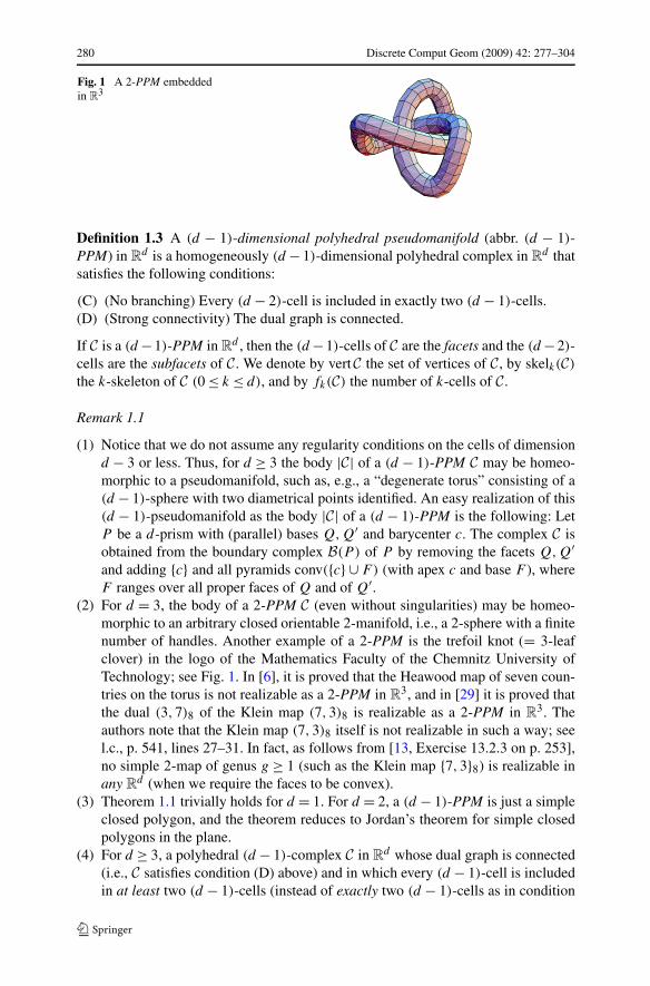
Fig. 1 A 2-PPM embeddedin R

3

Definition 1.3 A (d − 1)-dimensional polyhedral pseudomanifold (abbr. (d − 1)-PPM) in R

d is a homogeneously (d − 1)-dimensional polyhedral complex in Rd that

satisfies the following conditions:

(C) (No branching) Every (d − 2)-cell is included in exactly two (d − 1)-cells.(D) (Strong connectivity) The dual graph is connected.

If C is a (d −1)-PPM in Rd , then the (d −1)-cells of C are the facets and the (d −2)-

cells are the subfacets of C . We denote by vert C the set of vertices of C , by skelk(C)

the k-skeleton of C (0 ≤ k ≤ d), and by fk(C) the number of k-cells of C .

Remark 1.1

(1) Notice that we do not assume any regularity conditions on the cells of dimensiond − 3 or less. Thus, for d ≥ 3 the body |C| of a (d − 1)-PPM C may be homeo-morphic to a pseudomanifold, such as, e.g., a “degenerate torus” consisting of a(d − 1)-sphere with two diametrical points identified. An easy realization of this(d − 1)-pseudomanifold as the body |C| of a (d − 1)-PPM is the following: LetP be a d-prism with (parallel) bases Q,Q′ and barycenter c. The complex C isobtained from the boundary complex B(P ) of P by removing the facets Q,Q′and adding {c} and all pyramids conv({c} ∪ F) (with apex c and base F ), whereF ranges over all proper faces of Q and of Q′.

(2) For d = 3, the body of a 2-PPM C (even without singularities) may be homeo-morphic to an arbitrary closed orientable 2-manifold, i.e., a 2-sphere with a finitenumber of handles. Another example of a 2-PPM is the trefoil knot (= 3-leafclover) in the logo of the Mathematics Faculty of the Chemnitz University ofTechnology; see Fig. 1. In [6], it is proved that the Heawood map of seven coun-tries on the torus is not realizable as a 2-PPM in R

3, and in [29] it is proved thatthe dual (3,7)8 of the Klein map (7,3)8 is realizable as a 2-PPM in R

3. Theauthors note that the Klein map (7,3)8 itself is not realizable in such a way; seel.c., p. 541, lines 27–31. In fact, as follows from [13, Exercise 13.2.3 on p. 253],no simple 2-map of genus g ≥ 1 (such as the Klein map {7,3}8) is realizable inany R

d (when we require the faces to be convex).(3) Theorem 1.1 trivially holds for d = 1. For d = 2, a (d − 1)-PPM is just a simple

closed polygon, and the theorem reduces to Jordan’s theorem for simple closedpolygons in the plane.

(4) For d ≥ 3, a polyhedral (d − 1)-complex C in Rd whose dual graph is connected

(i.e., C satisfies condition (D) above) and in which every (d − 1)-cell is includedin at least two (d − 1)-cells (instead of exactly two (d − 1)-cells as in condition


Fig. 2 Simplified Bing’s house

(C) above), the complement Rd \ C may be connected, as the following example

shows.

Example 1.1 (Simplified Bing’s house with two rooms) Begin with the boundary ofa 3-cube, to which we add in the middle a horizontal (2-dimensional square) barrier(Fig. 2(a)). So far this is a polyhedral 2-dimensional complex which separates R

3

into three components (the exterior and two floors inside).Next make a square hole near the “north-west” corner of the upper ceiling, just be-

low it we make a parallel hole in the middle ceiling, and between these two holes forma “chimney” in the upper floor by adding four vertical panels as shown in Fig. 2(b).

A person standing on the roof may fall now into the lower storey through the chim-ney. Repeat the construction symmetrically near the opposite “south-east” corner inthe lower floor. The polyhedral 2-complex C obtained (see Fig. 2(c)) has a connecteddual graph, every edge of C is contained in at least two facets, and C does not separateR

3, i.e., R3 \ |C| is connected. This example easily generalizes to d ≥ 3.

(5) It is well known that if γ is a simple closed polygon in R2, then γ ∪ intγ can

be triangulated without adding vertices (see, e.g., [15], pp. 286–287). This doesnot generalize to (d − 1)-PPM’s in R

d for d ≥ 3, i.e., there is a 2-PPM C inR

3 such that C ∪ int C cannot be tetrahedrized without additional vertices. Twosuch 2-PPM’s in R

3 are presented in Sect. 5 below. But other results based onthe piecewise Jordan separation theorem may be generalized using Theorem 1.1,e.g., the characterization of those geometric graphs which are 1-skeletons of un-stacked triangulations of simple closed polygons given in [18].

For the sake of the proof of Theorem 1.1, we split our main theorem into twostatements, namely: Let C be a (d − 1)-PPM in R

d . Then

(E) Rd \ |C| is the disjoint union of two open sets, int C and ext C . The boundary of

each of these sets is |C|; int C is bounded, and ext C is unbounded.(F) The sets int C and ext C are (polygonally) connected.

We shall prove (E) in Sect. 2 by constructing a continuous function f : Rd \ |C| →

{0,1} which attains both values 0 and 1 in every neighborhood of every points x ∈ |C|,and defining ext C = f −1(0), int C = f −1(1). The (polygonal) connectedness of int Cand ext C is proved in Sect. 3 (see in particular Theorem 3.2).

Notation Bk(c, r) denotes the closed ball of dimension k centered at c and havingradius r .


2 A “Raindrop” Proof of (E)

The construction of f will be performed in four steps.

Step I: Choosing a “generic” direction.

Let F1, . . . ,Ft be all hyperplanes (= (d − 1)-flats) spanned by subsets of vert C . Fori = 1, . . . , t, let F 0

i =def Fi − Fi be the linear subspace parallel to Fi . Choose a unitvector v ∈ R

d \ ⋃ti=1 F 0

i (“v” for “vertical”). Vector v is our direction “up”, and −v

is pointing “down”.By the choice of v, a flat F spanned by vertices of C , other than R

d , will meet aline parallel to v in at most one point. For each point p ∈ R

d \ |C|, denote by R(p)

the closed vertical “pointing down” half-line R(p) =def {p − λv : 0 ≤ λ < ∞}. R(p)

is the path of a “raindrop” emanating from p. We divide Rd \ |C| into three disjoint

sets (recall that a subfacet means a (d − 2)-cell):

S0 = {p ∈ R

d \ |C| : R(p) does not meet any subfacet of C},

S1 = {p ∈ R

d \ |C| : R(p) meets exactly one subfacet of C},

S2 = {p ∈ R

d \ |C| : R(p) meets more than one subfacet of C}.

We shall first define f on S0 (= Step II), then extend its definition (continuously) toS1 (= Step III), and finally extend it (continuously) to S2 (= Step IV).

In the sequel, we shall use the following notation: For a set A ⊂ Rd , A+ =def

{a + λv : a ∈ A,λ ≥ 0}. A+ is the set of points of Rd that lie “above” A. Note that

(for all p ∈ Rd and A ⊂ R

d ):

R(p) meets A iff p ∈ A+. (1)

Step II: Define f on S0.

For p ∈ S0, denote by r(p) the number of facets (= (d − 1)-cells of C ) that meetR(p), and define f (p) =def

12 (1 − (−1)r(p)) to be the parity of r(p) (f (p) = 0 if

r(p) is even, 1 if r(p) is odd).Next we show that S0 is a dense open subset of R

d , and that f : S0 → {0,1} isa continuous, hence locally constant, function. In view of (1), we can write S0 =R

d \ (|C| ∪ |skeld−2 C|+), where |skeld−2 C| denotes the union of all subfacets of C .The set |skeld−2 C| is compact, same as C , and therefore |skeld−2 C|+ is closed. ThusS0 is an open subset of R

d . Moreover, the set |C| ∪ |skeld−2 C|+ can be covered by afinite number of hyperplanes in R

d . It follows that S0 is dense in Rd .

Now for the continuity of f . Assume x ∈ S0. Let ε be the (positive) distance fromx to |C| ∪ |skeld−2 C|+(= R

d \ S0). If x′ ∈ Rd,‖x − x′‖ < ε, then the segment [x, x′]

does not meet |C| ∪ |skeld−2 C|+. Let F be any facet of C . The set F+ is a closed,convex, unbounded and full-dimensional polyhedral subset of R

d whose boundaryconsists of the base F and of the side facets G+, where G ranges over all (d − 2)-faces of F . Thus, bdF+ ⊂ |C| ∪ |skeld−2 C|+, and therefore the segment [x, x′] doesnot meet the boundary of F+. It follows that x′ ∈ F+ iff x ∈ F+, i.e., R(x) meetsF iff R(x′) meets F . This is true for all facets F of C . Therefore, r(x) = r(x′),


hence f (x′) = f (x). Thus we have shown that the function f : S0 → {0,1} is locallyconstant, hence continuous.

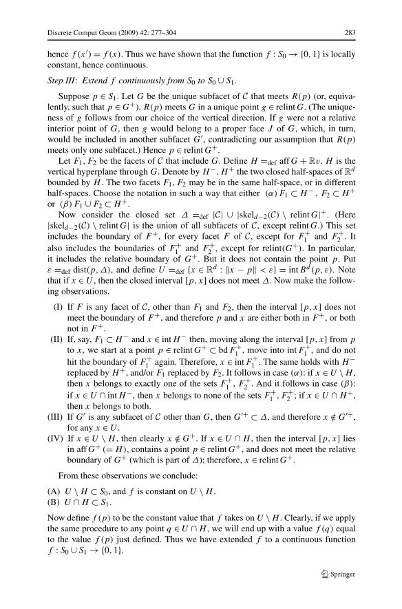
Step III: Extend f continuously from S0 to S0 ∪ S1.

Suppose p ∈ S1. Let G be the unique subfacet of C that meets R(p) (or, equiva-lently, such that p ∈ G+). R(p) meets G in a unique point g ∈ relintG. (The unique-ness of g follows from our choice of the vertical direction. If g were not a relativeinterior point of G, then g would belong to a proper face J of G, which, in turn,would be included in another subfacet G′, contradicting our assumption that R(p)

meets only one subfacet.) Hence p ∈ relintG+.Let F1,F2 be the facets of C that include G. Define H =def affG + Rv. H is the

vertical hyperplane through G. Denote by H−,H+ the two closed half-spaces of Rd

bounded by H . The two facets F1,F2 may be in the same half-space, or in differenthalf-spaces. Choose the notation in such a way that either (α)F1 ⊂ H− , F2 ⊂ H+or (β)F1 ∪ F2 ⊂ H+.

Now consider the closed set Δ =def |C| ∪ |skeld−2(C) \ relintG|+. (Here|skeld−2(C) \ relintG| is the union of all subfacets of C , except relintG.) This setincludes the boundary of F+, for every facet F of C , except for F+

1 and F+2 . It

also includes the boundaries of F+1 and F+

2 , except for relint(G+). In particular,it includes the relative boundary of G+. But it does not contain the point p. Putε =def dist(p,Δ), and define U =def {x ∈ R

d : ‖x − p‖ < ε} = intBd(p, ε). Notethat if x ∈ U , then the closed interval [p,x] does not meet Δ. Now make the follow-ing observations.

(I) If F is any facet of C , other than F1 and F2, then the interval [p,x] does notmeet the boundary of F+, and therefore p and x are either both in F+, or bothnot in F+.

(II) If, say, F1 ⊂ H− and x ∈ intH− then, moving along the interval [p,x] from p

to x, we start at a point p ∈ relintG+ ⊂ bdF+1 , move into intF+

1 , and do nothit the boundary of F+

1 again. Therefore, x ∈ intF+1 . The same holds with H−

replaced by H+, and/or F1 replaced by F2. It follows in case (α): if x ∈ U \ H ,then x belongs to exactly one of the sets F+

1 , F+2 . And it follows in case (β):

if x ∈ U ∩ intH−, then x belongs to none of the sets F+1 ,F+

2 ; if x ∈ U ∩ H+,then x belongs to both.

(III) If G′ is any subfacet of C other than G, then G′+ ⊂ Δ, and therefore x /∈ G′+,for any x ∈ U .

(IV) If x ∈ U \ H , then clearly x /∈ G+. If x ∈ U ∩ H , then the interval [p,x] liesin affG+ (= H), contains a point p ∈ relintG+, and does not meet the relativeboundary of G+ (which is part of Δ); therefore, x ∈ relintG+.

From these observations we conclude:

(A) U \ H ⊂ S0, and f is constant on U \ H .(B) U ∩ H ⊂ S1.

Now define f (p) to be the constant value that f takes on U \H . Clearly, if we applythe same procedure to any point q ∈ U ∩ H , we will end up with a value f (q) equalto the value f (p) just defined. Thus we have extended f to a continuous functionf : S0 ∪ S1 → {0,1}.


Step IV: Extend f continuously from S0 ∪ S1 to S0 ∪ S1 ∪ S2 (= Rd \ |C|).

Assume p ∈ S2. Then the ray R(p) meets at least two subfacets of C . (This canhappen only for d ≥ 3, by our choice of v.) Assume that R(p) meets exactly t distinctsubfacets G1, . . . ,Gt of C, t ≥ 2. Denote by G the subcomplex of C that consists ofall cells that do not meet R(p). Then p /∈ |C|∪|G|+. Define ε =def dist(p, |C|∪|G|+),and let U =def Bd(p, ε) ⊂ R

d (the open ball of radius ε centered at p). By our choiceof ε, we have S2 ∩ U = ⋃t

i=1⋃t

j=i+1(G+i ∩ G+

j ∩ U). In Lemma 2.1 below, we

will show that each of the sets G+i ∩ G+

j (1 ≤ i < j ≤ t) is included in a (d − 2)-flat. This will imply (see Lemma 2.2 below) that the union of these sets does notseparate U . The integer valued function f , defined and continuous on the connectedset (S0 ∪ S1) ∩ U (= U \ ⋃t

i=1⋃t

j=i+1(G+i ∩ G+

j ), takes a constant value c (c = 0or c = 1) there. We define f (p) to be c as well. This rule, applied to any other pointq ∈ S2 ∩ U , will assign to q the same value f (q) = c. Thus we have extended f to acontinuous (hence locally constant) function from S0 ∪S1 ∪S2 (= R

d \ |C|) to {0,1}.To complete the proof of statement (E), we define, as indicated above, the sets

ext C =def f −1(0) and int C =def f −1(1). These are clearly two disjoint open sets inR

d , whose union is domf = Rd \ |C|. Note that R

d \ conv |C| ⊂ ext C , and thereforeint C ⊂ conv |C|. Thus ext C is unbounded, and int C is bounded.

We still have to show that every point of |C| is a common boundary point of int Cand ext C (and therefore int C �= ∅, ext C �= ∅). Since the boundaries of int C and ofext C are closed sets, it suffices to show that the common boundary points of int C andext C are dense in |C|. If G is a subfacet (= (d − 2)-face) of C , then the set G+ Rv isincluded in a vertical hyperplane, and therefore intersects a facet F of C in a convexset of dimension ≤ d − 2. Thus F \ ∪{G + Rv : G ∈ skeld−2 C} is dense in F , and|C| \ (Rv + |skeld−2 C|) is dense in |C|. If x ∈ |C| \ (Rv + |skeld−2 C|), then x belongsto the relative interior of some facet F of C . If ε > 0 is sufficiently small, then thepoints x + εv, x − εv are both in S0, the ray R(x + εv) meets F , in addition to allfacets met by R(x−εv). Thus r(x+εv) = 1+r(x−εv), and f (x+εv) �= f (x−εv),i.e., {f (x − εv), f (x + εv)} = {0,1}. Thus x is a common boundary point of int Cand ext C .

Lemma 2.1 For 1 ≤ i < j ≤ t we have dim (G+i ∩ G+

j ) ≤ d − 2.

Proof Case I. If G+i ∩ G+

j = (Gi ∩ Gj)+, then

dim(G+

i ∩ G+j

) = dim(Gi ∩ Gj)+ = 1 + dim(Gi ∩ Gj) ≤ 1 + (d − 3) = d − 2.

(The intersection of two distinct (d − 2)-cells of C is a cell of C , of dimension ≤d − 3.)

Case II. G+i ∩ G+

j � (Gi ∩ Gj)+.

This means that we can find a point q that lies above a point q ′ ∈ Gi , andabove a point q ′′ ∈ Gj,q

′ �= q ′′. Thus q ′ = q − λ′v, q ′′ = q − λ′′v, λ′ > 0, λ′′ > 0,λ′ �= λ′′. The sets (affGi )+ and (affGj )+ are both (d − 1)-flats. If they are distinct,then G+

i ∩ G+j is included in their intersection, which is a (d − 2)-flat. There re-

mains the possibility that (affGi )+ = (affGj )+ =def H . If this happens, then the set


W =def vertGi ∪ vertGj is included in the (d − 1)-flat H , and the difference set ofaffW contains the vector q ′ − q ′′ = (λ′ − λ′′)v, contrary to our choice of v. �

Lemma 2.2 Let U ⊂ Rd be a convex set with non-empty interior (dimU = d). For

i = 1, . . . , t , let Ji be a (d − 2)-flat in Rd , and let Si be a subset of Ji . Then the

set T =def U \ ⋃ti=1 Si is polygonally connected. In fact, T is an L2-set (every two

points of T can be joined by a polygonal path in T with at most two edges).

Proof Assume a, b ∈ T . If [a, b] ⊂ T , we are done. Otherwise define, for i =1, . . . , t , Ai =def aff(Ji ∪ {a}), Bi =def aff(Ji ∪ {b}). Ai and Bi are flats of dimen-sion d − 1 or d − 2.

Since dimU = d , we can find a point c ∈ U \ ⋃ti=1(Ai ∪ Bi). In fact, we can

find such a point c arbitrarily close to 12 (a + b). If the line aff(a, c) meets Ji at

some point x other than a, then c ∈ aff(a, x) ⊂ aff({a} ∪ Ji) = Ai , contrary to ourchoice of c. Therefore, ]a, c] ∩ Ji = ∅ for i = 1, . . . , t , hence ]a, c] ⊂ U \ ⋃t

i=1 Ji ⊂U \ ⋃t

i=1 Si = T (so [a, c] ⊂ T ). The same argument, with a and Ai replaced by b

and Bi , shows that [c, b] ⊂ T . �

Remark 2.1 Lemma 2.2 can be extended beyond the realm of convex sets, as follows:If U is an open connected set in R

d , and S1, . . . , St are subsets of U withdim affSi ≤ d − 2 for i = 1, . . . , t , then the set T = U \ ⋃t

i=1 Si is polygonallyconnected. If two points a, b ∈ T can be joined by a polygonal path with n edgeswithin S, then they can be joined by a polygonal path with at most max(2, n) edgeswithin T . The proof is similar.

3 Polygonal Connectedness of intC and of extC

In this section we show that the open sets int C and ext C are (polygonally) connected.For any two points a, b ∈ int C , we construct a polygonal path from a to b that liesentirely in int C , stays mostly close to |C| and far from |skeld−3 C|. We do similarlyfor ext C . We shall also bound from above the number of edges of the constructedpaths. The bound will be approximately n

d, where n =def fd−1(C) is the number of

facets of C .

3.1 Some Preliminary Lemmata

Let the facets of C be F1, . . . ,Fn (n = fd−1(C)). For i = 1, . . . , n, let ui be a unitvector perpendicular to affFi . Choose the direction of ui in such a way that for eachpoint b ∈ relintFi and for all sufficiently small positive values of ε, b + εui ∈ ext Cand b − εui ∈ int C . If a subfacet G of C is the intersection of Fi and Fj (1 ≤ i <

j ≤ n), define uij =def ui + uj .

Lemma 3.1 If g ∈ relintG and ε is a sufficiently small positive number, then g +εuij ∈ ext C, g − εuij ∈ int C .


Fig. 3 Proof of Lemma 3.1

Proof The set affG is a (d − 2)-flat. Denote by A the (d − 2)-dimensional lin-ear subspace of R

d parallel to affG. (A = affG − affG and affG = g + A.) Thefacets Fi and Fj lie in two half-hyperplanes Hi and Hj bounded by affG, say,Hi = coneg(Fi) = affG + R

+vi,Hj = conegFj = affG + R+vj , where vi and vj

are suitable unit vectors in the orthogonal complement A+ of A. If ε is a sufficientlysmall positive number (0 < ε < dist(g, |C \ {Fi,Fj ,G}|)), then Bd(g, ε) \ |C| =Bd(g, ε) \ (Hi ∪ Hj). The union Hi ∪ Hj divides Bd(g, ε) into two open wedges,Bd(g, ε) ∩ int C and Bd(g, ε) ∩ ext C . If Hi and Hj lie in the same hyperplane(vj = −vi), then each of these two wedges is an open half-ball. In this case, ui = uj

(Fig. 3(a)), uij = 2ui = 2uj , and the lemma holds trivially. If ui and uj lie in dif-ferent hyperplanes, then one of the wedges is larger than a half-ball, and the other issmaller.

In all cases we have

〈ui, vj 〉 = 〈uj , vi〉 = sinα, (2)

where α is the dihedral angle of the wedge Bd(g, ε) ∩ ext C at g. If 〈ui, vj 〉 < 0, thenB(g, ε)∩ ext C is the larger wedge (Fig. 3(b)), and if 〈ui, vj 〉 > 0, then B(g, ε)∩ int Cis the larger wedge (Fig. 3(c)). Adding the equations ui = 〈ui, uj 〉uj +〈ui, vj 〉vj anduj = 〈uj ,ui〉ui + 〈uj , vi〉vi and using (2), we find that (1 − 〈ui, uj 〉) (ui + uj ) =sinα(vi + vj ).

If ui �= uj , then 1 − 〈ui, uj 〉 > 0, and therefore uij = ui + uj = sinα1−〈ui ,uj 〉 ×

(vi + vj ). Thus uij is a positive (resp., negative) multiple of vi + vj when sinα > 0(resp., sinα < 0). In both cases, uij points towards ext C , and −uij towards int C . �

Lemma 3.2 (“Push away from |C|”)

(a) Suppose Fi is a facet of C,G = Fi ∩ Fj is a subfacet, b ∈ relintFi, g ∈ relintG,and u is a vector that satisfies 〈u,ui〉 > 0. Define I0 =def [b,g], Iε =def [b +εu,g + εuij ] (ui, uj and uij = ui + uj denote the same vectors as in the pre-ceding lemma). If ε is a sufficiently small positive number, then Iε ⊂ ext C, I−ε ⊂int C . (The required smallness of ε may depend on the choice of the points b,g

and of the vector u.)(b) Suppose Fi,Fj ,Fk are distinct facets of C,G = Fi ∩ Fj ,H = Fj ∩ Fk are

subfacets (G �= H), g ∈ relintG,h ∈ relintH . Define J0 =def [g,h], Jε =def[g + εuij , h + εujk]. If ε > 0 is sufficiently small, then Jε ⊂ ext C and J−ε int C .

Proof (a) First note that I0 does not meet any facet of C except Fi and Fj . The sameholds for Iε , provided |ε| < min( 1

2 , 1‖u‖ ) · dist(I0, |C \ {Fi,Fj ,G}|). By Lemma 3.1


above, g + εuij ∈ ext C and g − εuij ∈ int C , provided ε is positive and sufficientlysmall. To complete the proof, it suffices to show that Iε ∩Fi = ∅ and Iε ∩Fj = ∅ (forsufficiently small |ε|, ε �= 0).

As for Fi : 〈ui, u〉 > 0 (given) and 〈ui, uij 〉 = 1 + 〈ui, uj 〉 > 0. Therefore, for anyε �= 0 both endpoints of Iε lie (strictly) on the same side of the hyperplane affFi ,hence Fi ∩ Iε = ∅.

As for Fj : If Fj and Fi lie in the same hyperplane (ui = uj ), then the pre-vious argument shows that Fj ∩ Iε = ∅ for all ε �= 0 as well. If ui �= uj , con-sider first the case where 〈ui, vj 〉 < 0 (Fig. 3(b)). For ε > 0, Iε lies in the openhalf-space {x ∈ R

d : 〈ui, x〉 > 〈ui, g〉}, whereas Fj lies in the closed half-space{x ∈ R

d : 〈ui, x〉 ≤ 〈ui, g〉}. Therefore, Iε ∩ Fj = ∅. For ε < 0, 〈uj , g + εuij 〉 =〈uj , g〉 + ε(1 + 〈ui, uj 〉) < 〈uj , g〉. On the other hand, 〈uj , b〉 < 〈uj , g〉 (for anypoint b ∈ relintFi , since 〈uj , vi〉 < 0), and therefore 〈uj , b + εu〉 < 〈uj , g〉 for suf-ficiently small |ε|, ε �= 0. Thus both endpoints of Iε lie on the same open side of thehyperplane affFj , hence Iε ∩ Fj = ∅.

In the case where 〈ui, vj 〉 > 0 (Fig. 3(c) above), just repeat the previous argumentwith the roles of ε > 0 and ε < 0 interchanged.

(b) The proof is similar to that of (a). First, note that J0 does not meet any facetof C except Fi,Fj , and Fk . The same holds for Jε provided |ε| < 1

2 · dist(J0, |C \{Fi,Fj ,Fk,G,H }|). By Lemma 3.1 above, g + εuij , h + εujk ∈ ext C and g −εuij , h − εujk ∈ int C , provided ε is positive and sufficiently small. To complete theproof, it suffices to show that Jε ∩ Fi = ∅, Jε ∩ Fj = ∅, and Jε ∩ Fk = ∅ (for suffi-ciently small |ε|, ε �= 0.

As for Fj : 〈uj ,uij 〉 = 1 + 〈uj ,ui〉 > 0 and 〈uj ,ujk〉 = 1 + 〈uj ,uk〉 > 0. There-fore, for any ε �= 0, both endpoints of Jε lie on the same open side of the hyperplaneaffFj , hence Fj ∩ Jε = ∅.

As for Fi : If Fj and Fi lie in the same hyperplane (ui = uj ), then the previousargument shows that Fi ∩ Jε = ∅ for all ε �= 0 as well. If ui �= uj , consider first thecase 〈ui, vj 〉 < 0 (Fig. 3(b) above). For ε > 0, Jε lies in the open half-space {x ∈R

d : 〈uj , x〉 > 〈uj , g〉}, whereas Fi lies in the closed half-space {x ∈ Rd : 〈uj , x〉 ≤

〈uj , g〉}. Therefore, Jε ∩ Fi = ∅. For ε < 0, we have 〈ui, g + εuij 〉 = 〈ui, g〉 + ε(1 +〈ui, uj 〉) < 〈ui, g〉. On the other hand, 〈ui, h〉 < 〈ui, g〉 (for any point h ∈ Fj \ G,since 〈ui, vj 〉 < 0), and therefore 〈ui, h + εujk〉 < 〈ui, g〉 for sufficiently small |ε|.Thus both endpoints of Jε lie on the same open side of the hyperplane affFi , henceJε ∩ Fi = ∅.

In the case where 〈ui, vj 〉 > 0 (Fig. 3(c) above), just repeat the previous argumentwith the roles of ε > 0 and ε < 0 interchanged.

As for Fk : Since the roles of Fi and Fk are interchangeable, the statement provedabove for Fi applies to Fk as well. �

Definition 3.1 Let p be a point in Rd \ |C| (= ext C ∪ int C ), and F be a facet of C .

We say that p sees F if, for some point a ∈ relintF, [p,a] ∩ |C| = {a}.

Lemma 3.3 Assume p ∈ Rd \ |C|. Then p sees at least one facet of C .

Proof Assume, w.l.o.g., that p ∈ ext C . Let q be a point in int C . Let U be a neighbor-hood of q that lies entirely in int C . Choose a point q ′ ∈ U such that the line aff(p, q ′)


does not meet any subfacet of C . (This condition can be met by avoiding a finite num-ber of hyperplanes through p.) Then the line segment [p,q ′] must meet |C|. Let a bethe first point of |C| on [p,q ′] (starting from p). Then a is a relative interior point ofsome facet F of C ; and [p,a] ∩ |C| = {a}. �

Definition 3.2 Let p be a point in Rd \ |C|. We say that p has a bounded horizon

(“does not see the sky”) with respect to C if every ray in Rd that emanates from p

meets |C|. (This is always the case when p ∈ int C .) Otherwise we say that p has anunbounded horizon. Of course, p can be of unbounded horizon only if p ∈ ext C .

Proposition 3.1 If p has a bounded horizon, then p sees at least d + 1 differentfacets of C .

Proof By Lemma 3.3, p sees at least one facet of C . Assume we know that p sees k

facets F1, . . . ,Fk of C , 1 ≤ k ≤ d . Choose points ai ∈ relintFi , 1 ≤ i ≤ k, such that[p,ai] ∩ |C| = {ai}, and unit vectors ui such that 〈ui, x〉 = 〈ui, ai〉 for all x ∈ Fi , and〈ui,p〉 < 〈ui, ai〉. (If p ∈ int C , then our vectors ui are the same as the vectors ui

defined before Lemma 3.1 above. If p ∈ ext C , then our vectors ui are the negativesof the vectors ui defined before Lemma 3.1.)

If k < d , or if k = d and the vectors u1, . . . , ud are linearly dependent, let w bea unit vector that is orthogonal to u1, . . . , uk . If k = d and the vectors u1, . . . , ud

are linearly independent, let w be a unit vector that satisfies 〈ui,w〉 < 0 for i =1, . . . , d . By our choice of w, the ray R(p,w) = {p + λw : λ ≥ 0} does not meet anyof the facets F1, . . . ,Fk . Since these facets are bounded, the same holds for the rayR(p,w′), provided w′ is sufficiently close to w. Choose w′ close to w and such thatthe ray R(p,w′) does not meet any subfacet of C . Let ak+1 be the first point of |C| onR(p,w′). The point ak+1 belongs to the relative interior of a facet Fk+1 of C . Clearly,p sees Fk+1, and Fk+1 is not one of the previous facets F1, . . . ,Fk . �

3.2 d-Connectedness of the Dual Graph of C

Theorem 3.1 (Generalized Balinski–Klee Theorem) If C is a (d − 1)-PPM (d ≥ 2),then the dual graph D(C) of C is d-connected.

Remarks (1) For the definition of a (d −1)-PPM, see Definitions 1.2 and 1.3 above.Theorem 3.1 does not make use of the assumption that the complex C lies in R

d ;C may lie in R

d ′for some d ′ > d . In fact, Theorem 3.1 can be stated for abstract

polyhedral pseudomanifolds (that might, or might not be realizable).(2) The theorem generalizes Balinski’s Theorem on the d-connectedness of the

graph (and of the dual graph) of a d-polytope (see [5] or [13, p. 213]). In fact, theproof given below uses Balinski’s Theorem. For simplicial (d − 1)-pseudomanifoldsTheorem 3.1 was formulated and proved by V. Klee; see [16, Theorem 5].

Proof Note that if d = 2, then the 1-PPM C is just a simple closed polygon, andthe dual graph of C is a simple circuit, which is 2-connected. Therefore, we assumein the sequel that d ≥ 3. In the sequel we denote the dual graph of C by D(C).


Given two facets A,B of C , a path (of length l) that connects A to B in D(C) isjust a sequence P = (F0,F1, . . . ,Fl) of facets of C that satisfies: F0 = A,Fl = B ,and dim(Fi−1 ∩ Fi) = d − 2 for i = 1, . . . , l. The facets F1, . . . ,Fl−1 are the inte-rior nodes of P . The path P is simple if the facets F0,F1, . . . ,Fl are all different.Since D(C) is a graph of valence ≥ d at each node, it has at least d + 1 nodes(fd−1(C) ≥ d + 1), and by the Menger–Whitney Theorem the d-connectedness ofD(C) is equivalent to the following claim. (The Menger–Whitney Theorem can beformulated as follows (see [30, p. 171]): A graph is k-connected iff every pair of ver-tices can be joined by at least k paths with pairwise disjoint interiors. The theoremgoes back to K. Menger (see [21] and [22]) and, independently, H. Whitney [34]; see[33]. The theorem is used in the proof of Balinski’s theorem; see [13, pp. 212–213],where it is attributed solely to Whitney, without mentioning his forerunner Menger.)

Claim 3.1 Given a list A,B,C1, . . . ,Cd−1 of d + 1 distinct facets of C , there is asimple path P in D(C) that connects A to B and avoids C1, . . . ,Cd−1.

Proof of Claim The existence of a simple path P in D(C) that connects A to B fol-lows by the assumption that D(C) is a connected graph (Condition (D) in Definition1.3). To prove the claim above we proceed by induction. Assuming we have a sim-ple path P in D(C) that connects A to B and avoids C1,C2, . . . ,Ck−1 (for somek, 1 ≤ k ≤ d − 1), we modify P to produce a simple path P ′ that avoids Ck as well.We shall need the following

Lemma 3.4 Let J be a (d − 3)-face of C . The subgraph of D(C) spanned by thefacets of C that include J is a disjoint union of simple circuits.

Proof of Lemma Every facet (= (d − 1)-face) of C that includes J has exactly twosubfacets (= (d −2)-faces) that include J . Conversely, every subfacet that includes J

is included in exactly two facets that include J (consider the no branching Condition(C) in Definition 1.3). In other words, the subgraph under consideration is 2-regular.Since it is finite, it must be a disjoint union of simple circuits. �

Back to the proof of Claim 3.1.Induction step k − 1 → k. Let P = (F0,F1, . . . ,Fl) be a simple path in D(C) that

connects A (= F0) to B (= Fl) and avoids C1, . . . ,Ck−1 (for some 1 ≤ k ≤ d − 1).If P avoids Ck as well, put P ′ = P . Otherwise assume Ck = Fj for some (unique) j

with 1 ≤ j ≤ l − 1.Define C =def Ck = Fj , G =def Fj−1 ∩ C, H =def C ∩ Fj+1. In the dual graph

of the (d − 1)-polytope C there are d − 1 simple paths π1, . . . , πd−1 with pair-wise disjoint interiors that connect the (d − 2)-faces G and H . This followsfrom the (d − 1)-connectedness of the dual graph of C (Balinski’s Theorem). Letπ = (Φ0,Φ1, . . . ,Φλ) with Φ0 = G and Φλ = H be one of those d − 1 paths(dim(Φi ∩ Φi+1 = d − 3 for 0 ≤ i ≤ λ − 1). π induces a path Π from Fj−1 toFj+1 in D(C) as follows. Each of the (d − 2)-faces Φi (0 ≤ i ≤ λ) is included inexactly two (d −1)-faces of C . One of them is C. Call the other one Qi . In particular,Q0 = Fj−1 and Qλ = Fj+1. For each i, 0 ≤ i < λ, the three (d − 1)-cells Qi , C and


Qi+1 share a (d − 3)-face Ψi =def Φi ∩ Φi+1. Thus 〈Qi,C,Qi+1〉 is an arc of oneof the circuits around J =def Ψi , as described in Lemma 3.4 above. The arc com-plementary to 〈Qi,C,Qi+1〉 within that circuit is an arc in D(C) that connects Qi

to Qi+1, avoids C, and uses only (d − 1)-cells that include Ψi . Concatenating thesecircumventing arcs from i = 0 to i = λ − 1, we obtain a path in D(C) that connectsFj−1 to Fj+1, and avoids C. We call this path Π . Applying this procedure to thepaths π1, . . . , πd−1, we obtain d − 1 paths Π1, . . . ,Πd−1 in D(C) that connect Fj−1to Fj+1 and avoid C.

Next we will show (Lemma 3.5 below) that two of these paths never share aninternal node (= (d − 1)-cell). Since the list C1, . . . ,Cd−1 of forbidden (d − 1)-cells contains, apart from C, only d − 2 additional cells, it follows that one of theavoiding paths, say Πν , does not use any of the forbidden (d − 1)-cells. Replace thearc 〈Fj−1,C,Fj 〉 in P by Πν , pass, if necessary, to a simple subpath, and call it P ′.P ′ is a simple path in D(C) from A to B that avoids C1, . . . ,Ck−1, and Ck .

Lemma 3.5 Let π,π ′ be two of the paths π1, . . . , πd−1 listed above, that connectG (= Fj−1 ∩ C) with H (= Fj+1 ∩ C) in the dual graph of C (say, π = πm,π ′ =πm′ , 1 ≤ m < m′ ≤ d − 1). Let Π and Π ′ be the paths induced by π and π ′, respec-tively, that connect Fj−1 to Fj+1 in D(C). Then Π and Π ′ have no internal node incommon.

Proof Assume π = (Φ0,Φ1, . . . ,Φλ), where Φ0 = Fj−1 ∩ C,Φλ = Fj+1 ∩ C, andeach Φi is a (d − 2)-face of C. Put Ψi =def Φi ∩ Φi+1 (i = 0,1, . . . , λ − 1). Each Ψi

is a (d − 3)-face of C. If Q is an internal node of the induced path Π , then Q ∩ C

is one of the (d − 2)-cells Φ1, . . . ,Φλ−1 or one of the (d − 3)-cells Ψ0, . . . ,Ψλ−1.The corresponding entities for π ′ are π ′ = (Φ ′

0, . . . ,Φ′λ′) (Φ ′

0 = Φ0,Φ′λ′ = Φλ), and

Ψ ′i = Φ ′

i ∩ Φ ′i+1 (i = 0,1, . . . , λ′ − 1).

If Q′ is an internal node of Π ′, then Q′ ∩ C is one of the cells Φ ′1, . . . ,Φ

′λ′−1 or

Ψ ′0, . . . ,Ψ

′λ′−1. To show that Q �= Q′, it suffices to check that the two sets {Φi : 1 ≤

i ≤ λ − 1} ∪ {Ψi : 0 ≤ i ≤ λ − 1} and {Φ ′i : 1 ≤ i ≤ λ′ − 1} ∪ {Ψ ′

i : 0 ≤ i ≤ λ′ − 1} aredisjoint. In fact, the Φ ′-s are different from the Φ-s, since π and π ′ have no internalnode in common. Each Ψi is included in exactly two (d − 2)-faces of C, which areadjacent nodes of π , and each Ψ ′

i′ is included in exactly two (d − 2)-faces of C,which are adjacent nodes of π ′. Since π and π ′ have no internal nodes in common,this implies that Ψi �= Ψ ′

i′ . Please pay attention to the possibility that, say, λ = 1, andΨ0 = Fj−1 ∩ C ∩ Fj+1. In this case, we necessarily have λ′ > 1, since π ′ �= π . �

This concludes the proof of Claim 3.1 and ends the proof of Theorem 3.1. ��

3.3 Upper Bounds for the Polygonal Diameter of int C and of ext C

Definition 3.3 For a set S ⊂ Rd and points a, b ∈ S, denote by πS(a, b) the smallest

number of edges of a polygonal line that connects a to b within S. (πS(a, b) =def ∞if no such polygonal line exists.) If S is polygonally connected, then πS(·, ·) is an in-teger valued metric on S. The polygonal diameter of S is defined as poldiam(S) =def


sup{πS(a, b) : a, b ∈ S}. Now we shall establish (almost) tight upper bounds for thepolygonal diameter of int C and of ext C , where C is a (d − 1)-PPM in R

d with n

facets. In Sect. 4 below, we shall present examples of polyhedral (d − 1)-spheresC, C′ in R

d with n facets (for all d ≥ 2 and d < n < ∞) such that poldiam(int C) =� n

d� , and poldiam(ext C′) = � n

d�. For d = 2, we shall even produce, in a subsequent

paper, such examples with C = C′ (see [25]). The following theorem clearly implies(F) in Sect. 1 above.

Theorem 3.2 (Upper bounds for poldiam(·)) If C is a polyhedral (d − 1)-pseudo-manifold (i.e., a (d−1)-PPM) with n facets in R

d , then the relations poldiam(int C) ≤2 + �n−2

d� and poldiam(ext C) ≤ 3 + �n−2

d� hold.

Proof Assume a, b are two points in the same component (int C or ext C ) of R \ |C|.We shall distinguish three possible cases.

Case I: Both a and b are of bounded horizon (with respect to C ) (cf. Definition 3.2above).

Case II: a is of bounded horizon, whereas b is of unbounded horizon (or viceversa).

Case III: Both a and b are of unbounded horizon.Denote by A(resp.,B) the set of those facets F of C such that a (resp., b) sees a

point in relintF via Rd \ |C|. By Proposition 3.1 above, we know that #A ≥ d + 1 if

a is of bounded horizon, and #A ≥ 1 otherwise (Lemma 3.3 above).If A ∩ B �= ∅, say F ∈ A ∩ B , then a sees a point a′ ∈ relintF and b sees a

point b′ ∈ relintF via Rd \ |C|. Choose points a′′ ∈ ]a, a′[ (close to a′) and b′′ ∈

]b, b′[ (close to b′), such that the segment [a′′, b′′] runs parallel to F and misses C .Then 〈a, a′′, b′′, b〉 is a 3-path that connects a to b via R

d \ |C|. The upper bounds inTheorem 3.2 are all ≥ 3, except for int C , when n = d + 1. But when n = d + 1, int Cis the interior of a d-simplex, which is convex. Assume, from now on, that A∩B = ∅,and consider each case separately.

Case I: In this case, #A ≥ d + 1,#B ≥ d + 1. Let D = D(C) be the dual graphof C . By Theorem 3.1, D is d-connected. Extend D to a graph D′′ by adding two(auxiliary) vertices, a and b, connecting a by edges to all members of A and b

to all members of B . As one can easily check, the extended graph D′′ is again d-connected. Therefore, in D′′ we can find d paths π1, . . . , πd that connect a to b andhave pairwise disjoint interiors. If we take these paths as short as possible (in par-ticular, diagonal free), then each πi will visit the set A (= neighbors of a) exactlyonce. Since #A ≥ d + 1 and #B ≥ d + 1, it follows that all these d paths togethervisit at most n − 2 vertices of D. The shortest of these paths, say π1, is of the form〈a,F1, . . . ,Fm,b〉, where m ≤ �n−2

d�,F1, . . . ,Fm are facets of C,Fi−1 and Fi share

a subfacet Gi for i = 2, . . . ,m, a sees via Rd \ |C| a point a′ ∈ relintF1, and b sees

via Rd \ |C| a point b ∈ relintFm. If we choose points gi ∈ relintGi for i = 2, . . . ,m,

then 〈a, a′, g2, g3, . . . , gm, b′, b〉 is a polygonal path of m + 2 edges that connects a

to b and runs along |C|. By Lemma 3.2, this path can be pushed away from |C|, thusproducing a polygonal path of m + 2 edges that connects a to b via R

d \ |C|.Case II: In this case, extend the graph D = D(C) to a graph D′ by adding the

(auxiliary) vertex a and connecting a by edges to all vertices in A. Fix a vertex


F ′ ∈ B . D′ is again d-connected and contains d paths π1, . . . , πd from a to F ′, withpairwise disjoint interiors. If we take these d paths to be diagonal free, then theirunion misses at least one vertex of A (recall #A ≥ d + 1). The union of their interiorsmisses F ′ as well, and thus uses at most n − 2 facets of C . The shortest of thesepaths, say π1, is of the form 〈a,F1, . . . ,Fm,F ′〉, where m ≤ �n−2

d�. As in Case I, this

path gives rise to a polygonal path 〈a, a′, g2, . . . , gm,gm+1, b′, b〉, with a′ ∈ relintF1,

gi ∈ relint(Fi−1 ∩ Fi) (i = 2, . . . ,m), gm+1 ∈ relint(Fm ∩ F ′), and b′ ∈ relintF ′, andthus to a polygonal path of at most 3 +�n−2

d� edges that connects a to b via R

d \ |C|.Case III: Denote by Ua (resp., Ub) the set of unit vectors u such that the ray

a + R+u (resp., b + R

+u) misses |C|. Since |C| is compact and a /∈ |C|, Ua is anopen subset of the unit sphere Sd−1 ⊂ R

d . We have Ua �= ∅, since a is of unboundedhorizon, and the same holds for Ub . Choose vectors ua ∈ Ua and ub ∈ Ub such thatub �= −ua . There is a linear function f that satisfies f (ua) = f (ub) = 1. Put M =defmax{f (x) : x ∈ |C|}. If t > M −min{f (a), f (b)}, then the segment [a+ tua, b+ tub]misses |C|, and 〈a, a+ tua, b+ tub, b〉 is a polygonal path of three edges that connectsa to b via R

d \ |C|. �

4 Lower Bounds for the Maximal Polygonal Diameter of the Interior andExterior of a (d − 1)-PPM in R

d

For n ≥ d + 1 > 0, define (note that poldiam(.) is defined in Definition 3.3 above):

pd-int(d,n) =def max{poldiam(int P ) : P is a (d−1)-PPM in R

d and fd−1(P ) = n}

(“pd” stands of “polygonal diameter”) and

pd-ext(d,n) =def max{poldiam(ext P ) : P is a (d − 1)-PPM in R

d

and fd−1(P ) = n}.

The following upper bounds were established in Theorem 3.2 above:

pd-int(d,n) ≤ 2 +⌊

n − 2

d

⌋

, (3)

pd-ext(d,n) ≤ 3 +⌊

n − 2

d

⌋

. (4)

In this section we produce two (d − 1)-PPMs P and Q in Rd , with fd−1(P ) =

fd−1(Q) = n, n ≥ d + 1 > 0, such that poldiam(int P ) = � nd� and poldiam(ext Q) =

� nd�. These examples establish lower bounds � n

d� (resp., � n

d�) for pd-int(d,n) (resp.,

pd-ext(d,n)) which are quite close to the upper bounds given in (3) (resp., (4)) above.

Example 4.1 (Zigzag sleeve) This is an example of a polyhedral (d − 1)-sphere P inR

d (i.e., combinatorially equivalent to the boundary complex of a convex polytopein R

d ) with n (≥ d + 1 > 0) facets such that poldiam(int P ) = m =def � nd�. Assume

first that n ≡ 0 (mod d), i.e., n = md , m ≥ 2. Let Δd−1 be a (d − 1)-simplex in Rd


Fig. 4 Example 4.1 for m = 5,d = 3

with barycenter at the origin o contained in the relative interior of the unit (d − 1)-ball Bd−1(o,1) of R

d−1, where Rd−1 =def {x = (ξ1, . . . , ξd) ∈ R

d : ξd = 0}, and letF1, . . . ,Fd be the facets of Δd−1. Define m + 1 points a0, a1, . . . , am by aν =def(−1)νed−1 + νed (ν = 0,1, . . . ,m). For ν = 1, . . . ,m, define a d-polytope Pν asfollows:

P1 =def conv({a0} ∪ (

a1 + Δd−1)),

Pν =def conv((

aν−1 + Δd−1) ∪ (aν + Δd−1)) = [aν−1, aν] + Δd−1

for 2 ≤ ν < m, and for ν = m we define Pm =def (conv(am−1 +Δd−1)∪{am}). Definealso P =def

⋃mν=1 Pν . P1 is a d-simplex (a d-pyramid based on a1 + Δd−1 apexed

at a0), Pν, 1 < ν < m, is a d-prism on a (d − 1)-simplex (the sum of the segment[aν−1, aν] and the simplex Δd−1), and Pm is a d-simplex (a d-pyramid based onam−1 + Δd−1 and apexed at am). The union P = P1 ∪ P2 ∪ · · · ∪ Pm is piecewiselinearly homeomorphic (as a transformation that changes the d-coordinate only, i.e.,a “piecewise shear” parallel to R

d−1) to a convex polytope which is a (d − 1)-prismon a (d − 1)-simplex with two d-simplices attached to its two bases, like a pencilsharpened at both ends (see Fig. 4 for m = 5, d = 3). (Such a convex polytope maybe called a bi-apexed prism.)

The boundary complex P of P consists of md (= n) convex (d − 1)-polytopes(2d (d − 1)-simplices and (m − 2) · d (d − 1)-prisms on (d − 2)-simplices), listedas follows:

conv({a0} ∪ (a1 + Fi)

), [aν−1, aν] + Fi (2 ≤ ν ≤ m − 1),

conv((am−1 + Fi) ∪ {am}),

all this for i = 1,2, . . . , d . All these (d − 1)-polytopes, together with all their faces,form a (d − 1)-PPM, henceforth denoted by P , satisfying int P = intP (here int Pis the interior of P in the sense of the Jordan–Brouwer separation theorem (Theo-rem 1.1 above) and intP is the (topological) interior of P as a (closed) set in R

d ).The following proposition implies that poldiam(int P ) = m.


Proposition 4.1 It is possible to proceed from any point q0 ∈ intBd(a0,1) ∩ intP(a 1-vicinity of a0 in intP ) to any point qm ∈ intBd(am,1) ∩ intP (a 1-vicinity ofam in intP ) by a polygonal path of m edges, but not by less than this.

Proof Define γ =def 〈q0, a1, a2, . . . , am−1, qm〉. γ is a polygonal path of m edges inintP from q0 to qm. This proves the first part of the proposition. To prove the secondpart, we give first an informal argument (see Fig. 4). In order to reach from q0 toP1 ∩ P2 (= a1 + Δd−1), there must be a decreasing segment (ξd−1 decreases as afunction of ξd ); in order to reach from P1 ∩ P2 to P2 ∩ P3 (= a2 + Δd−1), there mustbe an increasing segment (ξd−1 increases as a function of ξd ), etc.; finally, in order toreach from Pm−1 ∩ Pm to qm, there must be a decreasing [increasing] segment if m

is odd [if m is even]. This makes a zigzag of m edges.Formal proof. Among the polygonal paths from q0 to qm in intP , let γ be a polyg-

onal path of minimal number, say n, of edges, and let p0,p1, . . . , pn be its verticesin this order, i.e., γ = 〈p0 = q0,p1,p2, . . . , pn−1,pn = qm〉. (We have to show thatn ≥ m.) Note that the role played by n here is different from that played by n =deffd−1(C) defined supra.

We will think of γ as a (piecewise linear and continuous) function from [0,1] toR

d with γ (0) = q0 and γ (1) = qm. Since γ (0) = q0 �= qm = γ (1), γ is not a circuit.

Claim 4.1 γ is 1-1, i.e., γ is a simple path.

Proof of Claim If γ is not 1-1, then it contains a circuit, say γ : [t1, t2] → Rd with

[t1, t2] ⊂ [0,1], γ (t) = γ (t) for t ∈ [t1, t2] and γ (t1) = γ (t2). Reduce γ to [0, t1] ∪[t2,1] (i.e., drop the circuit γ from γ ). The resulting polygonal path connects q0to qm via intP and it clearly has fewer edges then γ , a contradiction. This provesClaim 4.1. �

For 1 ≤ i ≤ m − 1, define a vertex qi of γ as follows: Put ti =def max{t with0 ≤ t ≤ 1 : γd(t) = i} (ti is the last time that γ visits the hyperplane ξd = i). Clearly,γ (ti) ∈ ai + Δd−1 (= Pi ∩ Pi+1), hence

sg(γd−1(ti)

) = (−1)i , 1 ≤ i ≤ m − 1, (5)

and by Claim 4.1 above, γ (ti) ∈ [pι−1,pι[ for some unique ι = ι(i), 1 ≤ ι ≤ n. Define

qi =def

{pι−1 if sg((pι−1)d−1) = (−1)i ,

pι otherwise.

This definition ensures that

sg((qi)d−1

) = (−1)i(= sg(ai)

)(6)

for 0 ≤ i ≤ m. We will show that the vertices qi,0 ≤ i ≤ m, are all different.

Lemma 4.1 Let [u,v] be a segment contained in intP such that (u)d = i for some i

with 1 ≤ i ≤ m−1, (v)d �= i and [u,v]∩G = ∅, where G =def {x ∈ Rd : (x)d−1 = 0}.

Then either i − 1 < (v)d < i or i < (v)d < i + 1.


Proof of Lemma Put Gi =def {x ∈ Rd : sg(x)d−1 = (−1)i or 0}. Note that u ∈ ai +

Δd−1 (= Pi ∩Pi+1), hence Gi is the closed half-space bounded by G which containsu (and v).

The d-polytope Pi [Pi+1] is a d-prism if 1 < i ≤ m − 1 [1 ≤ i < m − 1], a d-simplex if i = 1 [i = m − 1]; and it is contained in the layer L−

i =def {x ∈ Rd : i −

1 ≤ (x)d ≤ i} [L+i =def {x ∈ R

d : i ≤ (x)d ≤ i + 1}]. The d-polytope Qi =def Pi ∩Gi [Qi+1 =def Pi+1 ∩ Gi] satisfies

intQi ⊂ intL−i

[intQi+1 ⊂ intL+

i

], (7)

and it has d +2 facets: d facets are subsets of the d facets of Pi [Pi+1] whose relativeinteriors are contained in intL−

i [intL+i ], henceforth called loxo facets, as well as the

two facets ai + Δd−1(= Pi ∩ Pi+1) and G ∩ Pi [G ∩ Pi+1]. If (v)d < i [i < (v)d ],then ]u,v] ∩ intQi �= ∅ [ ]u,v] ∩ intQi+1 �= ∅], and since ]u,v] does not intersectany of the d loxo facets of Pi [Pi+1] (since [u,v] ⊂ intP ) and it does not intersectthe facet G ∩ Pi [G ∩ Pi+1] (since [u,v] ∩ G = ∅), it follows that [u,v] ∩ bdQi =u [[u,v] ∩ bdQi+1 = u], hence v ∈ intQi [v ∈ intQi+1]. It follows from (7) thati − 1 < (v)d < i if (v)d < i [i < (v)d < i + 1 if i < (v)d ]. This proves Lemma 4.1. �

Claim 4.2 (q0)d < 1, m − 1 < (qm)d and for 1 ≤ i ≤ m − 1, i − 1 < (qi)d < i + 1.

Proof of Claim The first two inequalities follow from ‖q0 −a0‖ < 1 and ‖qm−am‖ <

1, respectively. Let 1 ≤ i ≤ m−1. If (qi)d = i, we are done. Assume (qi)d �= i. Usingthe notation introduced above, {γ (ti), qi} ⊂ intGi by (5) and (6), hence [γ (ti), qi] ∩G = ∅. Since γ (ti) ∈ Pi ∩ Pi+1, the segment [γ (ti), qi] satisfies the conditions ofLemma 4.1 above (with u = γ (ti)) and v = qi ), hence either i − 1 < (qi)d < i ori < (qi)d < i + 1, hence i − 1 < (qi)d < i + 1. This proves Claim 4.2. �

We show now that qi �= qj for 0 ≤ i < j ≤ m. If j and i are of different parities,this follows from (6). Let j = i + 2κ for some κ ≥ 1. In view of Claim 4.2,

(qi)d < i + 1 < (qi+2)d < i + 3 < (qi+4)d < · · · < i + (2κ − 1) < (qi+2κ )d ,

hence qi �= qi+2κ (= qj ). This concludes the proof of Proposition 4.1. �

It remains to modify Example 4.1 to the case where n �≡ 0 (mod d), i.e., n =md + r , 1 ≤ r ≤ d − 1. If r = 1, truncate the vertex am of P by a hyperplane pass-ing in an ε-vicinity of am for some sufficiently small ε > 0. The resulting body P ′has md + 1 (= n) facets, d new vertices and, clearly, if ε is small enough, thenpoldiam(intP ′) = poldiam(intP) = m = � n

d�. If r = 2, truncate P near am as above,

and then truncate P ′ near enough to one of its new vertices; the resulting body P ′′has md + 2 (= n) facets and again poldiam(intP ′′) = m = � n

d�. For 3 ≤ r ≤ d − 1

make, similarly, r truncations near am to obtain a body P (r) with md + r (= n) facetsand poldiam(intP (r)) = m = � n

d�.

Example 4.2 (Pyramid with a zigzag cave) Now we will modify the complex of Ex-ample 4.1 above to obtain a (d − 1)-PPM Q in R

d with n (≥ d + 1 > 0) facets


such that poldiam(ext Q) = � nd�. Again assume first that n ≡ 0 (mod d), i.e., n = md

(m ≥ 2). In this case, � nd� = m, so Q will have md facets, and poldiam(Q) = m.

Define m d-polytopes Q1, . . . ,Qm as follows:

(a) Qν =def Pν for 4 ≤ ν ≤ m.(b) Q2 =def conv((ed +M ·Δd−1)∪(a2(ε)+Δd−1)) with large enough M satisfying

±ed−1 + (ed +Δd−1) ⊂ relint

(ed +M ·Δd−1) (⊂ H =def

{x ∈ R

d : (x)d = 1})

,

(8)and a2(ε) =def ed−1 + (3 − ε)ed , where ε is a positive number whose smallnessis determined below. Since M ·Δd−1 is a homothetic image of Δd−1 and a2(ε)+Δd−1 is a translate of Δd−1, an easy calculation shows that ed + M · Δd−1 is

a homothet of a2(ε) + Δd−1 with center of homothety b =defa2(ε)− 1

Med

1− 1M

(and

constant of homothety M). Hence Q2 is combinatorially equivalent to a d-prismon a (d − 1)-simplex (same as conv((a1 + Δd−1)∪ (a2(ε)+ Δd−1))). The facetsGi =def conv((ed + MFi) ∪ (a2(ε) + Fi)),1 ≤ i ≤ d , of Q2 (recall that Fi,1 ≤i ≤ d , are facets of Δd−1) will be referred to below as the side facets of Q2.

(c) Q3 =def conv((a2(ε) + Δd−1) ∪ (a3 + Δd−1)). Q3 is a d-prism on a (d − 1)-simplex analogous to P3 above, where a2(ε) plays the role of a2 in the definitionof P3. The replacement of a2 by a2(ε) (where ε > 0 is small) flattens Q3 inthe d-axis direction (the d-axis difference between the two bases of the prism issmall).

(d) Q1 =def conv((ed +M ·Δd−1)∪ {a0(L)}), where a0(L) =def (L+ 1)ed and L isa positive number whose largeness is determined below.

First we determine M . Since Δd−1 ⊂ relintBd−1(o,1) (= the relative interior ofthe unit (d − 1)-ball centered at the origin o in the plane (x)d = 0) and sinceo ∈ relintΔd−1,

±ed−1 + Δd−1 ⊂ relintBd−1(o,2) (9)

(= the relative interior of the (d − 1)-ball of radius 2 centered in the origin in thehyperplane (x)d = 0). Clearly, Bd−1(o,2) ⊂ M · Δd−1 for

M >2

dist(o, relbdΔd−1), (10)

hence (8) follows from (9) provided M satisfies (10). So put

M =def2

dist(o, relbdΔd−1)+ 1.

Next we determine ε. (As mentioned above, the smallness of ε determines theflatness of Q3 in the d-axis direction.)

Put H =def {x ∈ Rd : (x)d = 1}, H− =def {x ∈ R

d : (x)d ≤ 1} and H− =(coneb(ed + M · Δd−1)) ∩ intH−. Our main concern in determining ε > 0 is

Requirement 4.1 (Smallness of ε > 0) For u ∈ H− and z+ ∈ a3 + Δd−1 the halfopen segment [u, z+[ avoids the basis a2(ε) + Δd−1 of Q3. In other words, it is


impossible to reach from a point in H− a point in the upper basis a3 + Δd−1 of Q3

directly by a segment via the lower basis a2(ε) + Δd−1 of Q3.We will show now the existence of such a (small) positive ε.Put G =def {x ∈ R

d : (x)d−1 = 0}, G− =def {x ∈ Rd : (x)d−1 ≤ 0}, G+ =def {x ∈

Rd : (x)d−1 ≥ 0}, and H3 =def {x ∈ R

d : (x)d = 3}.

Since a3 + Δd−1 ⊂ intG−, Requirement 4.1 will be met provided

(relint

(coneu

(z−))) ∩ H3 ⊂ G+ (11)

for u ∈ H− and z− ∈ a2(ε) + Δd−1. Consider the (parallel) (d − 2)-flats Fd−21 =def

3ed + span(e1, e2, . . . , ed−2) and Fd−20 =def ed + (M + 1)ed−1 + span(e1, e2,

. . . , ed−2).We have Fd−2

0 ‖Fd−21 ,F d−2

1 ⊂ H3 ∩ G and Fd−20 ⊂ H . Fd−2

0 is a hyperplaneof H strictly supporting ed + M · Δd−1 (⊂ H). Put I d−1 =def aff(F d−2

0 ∪ Fd−21 ).

The hyperplane I d−1 is the common boundary of two closed half-spaces I d−1− , I d−1+ ;choose the signs +,− so that ed + M · Δd−1 ⊂ I d−1− , so H3 ∩ G+ ⊂ I d−1+ . Defineδ =def dist(ed−1 +Δd−1,G); since the two sets involved in this definition are disjoint,ed−1 + Δd−1 is compact and G is closed, δ > 0. Let ε > 0 satisfy

ε

δ<

2

M + 1. (12)

The difference between Fd−20 and Fd−2

1 in the d-axis direction is 2, and their dif-ference in the (d − 1)-axis direction is M + 1. It follows that if ε satisfies (12),then a2(ε) + Δd−1 ⊂ I d−1+ , and Condition (11) is met by such an ε. So defineε =def

δM+1 (= 1

2 · 2δM+1 ). With this ε Requirement 4.1 is met. It remains to deter-

mine L.

Requirement 4.2 (Largeness of L) L > 0 is so large that

m⋃

ν=2

Qν ⊂ Q1. (13)

The existence of such an L can be easily verified by a glance on Fig. 5. For aformal proof put

A =def conv((

ed−1 + ed + Δd−1) ∪ (−ed−1 + ed + Δd−1)),

B =def conv(A ∪ (

(m − 1)ed+1 + A))

, and

δ1 =def dist(A, relbd

(ed + M · Δd−1)).

A is a (d − 1)-polytope, B is a right d-prism of height m − 1 on A contain-ing

⋃mν=2 Qν , and δ1 > 0 since A and ed + M · Δd−1 are compact and disjoint

(A ⊂ relint(ed + MΔd−1), by (8)). If L

dist(o,relbd(M·Δd−1))> m−1

δ1, then the segment


Fig. 5 A projection ofExample 4.2 on the(ed−1, ed )-plane for m = 5

between a0(L) = (L + 1)ed and any point in relbd(M · Δd−1) does not meet B;hence for

L >(m − 1) · dist(o, relbd(M · Δd−1))

δ1. (14)

Requirement 4.2 is satisfied. So define

L =def(m − 1) · dist(o, relbd(M · Δd−1))

δ1+ 1.

Having defined Q1, . . . ,Qm, put Q =def cl (Q1 \ ⋃mν=2 Qν). In view of (13), Q

is a zigzag hole drilled in Q1 from its basis ed + M · Δd−1 on (see Fig. 5), andthe boundary of Q is a polyhedral complex, henceforth denoted by Q, combinato-rially equivalent to the complex P of Example 4.1 above. Since bdQ = |Q| andintQ = int Q (here intQ is in the sense of the polyhedral Jordan–Brouwer separationtheorem (Theorem 1.1 above)), it follows that ext Q = R

d \ (Q ∪ int Q). (Here ext Qis in the sense of the polyhedral Jordan–Brouwer separation theorem (Theorem 1.1above).)

The following implies that poldiam(ext Q)= m (compare Proposition 4.1 above).

Proposition 4.2 It is possible to proceed via ext Q from any point q0 ∈ Rd \

(H− ∪ Q1) ⊂ ext Q to any point qm ∈ (intBd(am,1)) ∩ intQm ⊂ ext Q (a 1-vicinityof am in ext Q) by a polygonal path of m edges, but not by less than this.

Proof Let d ′ ∈ bdQ1 \ {a0(L)} satisfy [q0, d′] ∩ Q1 = {d ′}. Such a point exists

since q0 /∈ Q1. Since q0 /∈ H−, d ′ /∈ ed + M · Δd−1, and [q0, d′′] ∩ Q1 = {d ′′} for

all d ′′ ∈ conea0(L)d′. Let d ′′ ∈ (conea0(L)d

′) ∩ H−; then (coneq0 d ′′) ∩ int H− �=∅ and (coneq0d

′′) ∩ Q1 = ∅. Let q1 ∈ (coneq0d′′) ∩ int H−, and define γ =def

〈q0, q1, a2(ε), a3, a4, . . . , am−1, qm〉. Since [q0, q1] ∩ Q1 = ∅, γ is an m-gon fromq0 to qm via ext Q. This proves the first part of the proposition.

To prove the second part observe that any polygonal path from q0 to qm via ext Qmust reach a point q1 ∈ H− before entering the “zigzag cave”

⋃mν=2 Qν , which takes


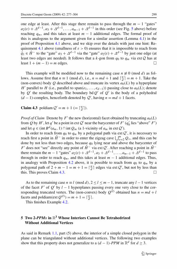
one edge at least. After this stage there remain to pass through the m − 1 “gates”a2(ε) + Δd−1, a3 + Δd−1, . . . , am−1 + Δd−1 in this order (see Fig. 5 above) beforereaching qm, and this takes at least m − 1 additional edges. The formal proof ofthis is analogous to the argument given for a similar assertion (Lemma 4.1) in theproof of Proposition 4.1 above, and we skip over the details with just one hint: Re-quirement 4.1 above (smallness of ε > 0) ensures that it is impossible to reach fromq1 ∈ H− to the “gate” a3 + Δd−1 via the “gate” a2(ε) + Δd−1 by just one edge (atleast two edges are needed). It follows that a k-gon from q0 to qm via ext Q has atleast 1 + (m − 1) = m edges. �

This example will be modified now to the remaining case n �≡ 0 (mod d) as fol-lows. Assume first that n ≡ 1 (mod d), i.e., n = md + 1 and � n

d� = m + 1. Take the

(non-convex) body Q described above and truncate its vertex a0(L) by a hyperplaneH ′ parallel to H (i.e., parallel to span(e1, . . . , ed−1)) passing close to a0(L); denoteby Q′ the resulting body. The boundary bdQ′ of Q′ is the body of a polyhedral(d − 1)-complex, henceforth denoted by Q′, having n = md + 1 facets.

Claim 4.3 poldiam Q′ = m + 1 (= � nd�).

Proof of Claim Denote by F ′ the new (horizontal) facet obtained by truncating a0(L)

from Q by H ′, let q ′ be a point in ext Q′ near the barycenter of F ′ (q ′0 lies “above” F ′)

and let q ∈ (intBd(am,1) ∩ intQm (a 1-vicinity of am in ext Q′).In order to reach from q0 to qm by a polygonal path via ext Q′, it is necessary to

reach first a point in H− in order to enter the zigzag cave⋃m

ν=2 Qν , and this can bedone by not less than two edges, because q0 lying near and above the barycenter ofF ′ does not “see” directly any point of H− via ext Q′. After reaching a point in H−there remain the m − 1 “gates” a2(ε) + Δd−1, a3 + Δd−1, . . . , am−1 + Δd−1 to passthrough in order to reach qm, and this takes at least m − 1 additional edges. Thus,in analogy with Proposition 4.2 above, it is possible to reach from q0 to qm by apolygonal path of 2 + m − 1 = m + 1 = � n

d� edges via ext Q′, but not by less than

this. This proves Claim 4.3. �

As to the remaining case n ≡ l (mod d),2 ≤ l ≤ m− 1, truncate any l − 1 verticesof the facet F ′ of Q′ by l − 1 hyperplanes passing every one very close to the cor-responding truncated vertex. The (non-convex) body Q(l) obtained has n = md + l

facets and poldiam(extQ(l)) = m + 1 = � nd�.

This finishes Example 4.2.

5 Two 2-PPMs in R3 Whose Interiors Cannot Be Tetrahedrized

Without Additional Vertices

As said in Remark 1.1, part (5) above, the interior of a simple closed polygon in theplane can be triangulated without additional vertices. The following two examplesshow that this property does not generalize to a (d − 1)-PPM in R

d for d ≥ 3.


Fig. 6 The six basic rectangularpanels of Example 5.2

Example 5.1 The first example is the famous Schönhardt’s twisted prism over a tri-angle, which is a simplicial 2-manifold C in R

3 with six vertices combinatoriallyequivalent to the boundary complex of the 3-octahedron, first described in [28]. It isobtained from a 3-prism on a triangular basis by a (small), say clockwise, twist of oneof the two bases. The three quadrilateral facets are thus broken at their three mutuallydisjoint diagonals and “bent in” so that the three dihedral angles at these three diag-onals become concave (i.e., >π ). The relative interiors of the other three diagonalsare thus “pushed out” to lie entirely in ext C . Clearly, any tetrahedron whose verticesare in vert C must have as an edge one of these three “outside diagonals”. It followsthat int C ∪ C cannot be tetrahedrized without additional vertices. This example wasrecently generalized in [27] to a twisted prism over any (convex) polygon, and muchearlier it was generalized by [4] in a different, yet very simple direction. In [27], onecan also find further discussion and references on this subject.

Let us present now another example which turns out to be combinatorially equiva-lent to the so called rhombicuboctahedron. Later on we shall see that, although Schön-hardt’s polyhedron is much simpler than our example below, this example is perhapsnot devoid of interest because of another tetrahedrization-obstructing property it hasover Schönhardt’s and its generalizations described above.

Example 5.2 The idea is to put some mutually disjoint 2-dimensional rectangularpanels M1, . . . ,Mk in R

3 such that o ∈ R3 \⋃k

i=1 Mi and every segment [o, v], wherev is a vertex of some panel Mi (1 ≤ i ≤ k), meets another panel Mj (1 ≤ j ≤ k,j �= i), i.e., o does not “see” any vertex of

⋃ki=1 Mi , and then to complete

{M1, . . . ,Mk} to a 2-PPM C by adding facets without additional vertices (i.e.,vert C = ⋃k

i=1 vertMi ) so that o ∈ int C . The interior int C of such a 2-PPM can-not be tetrahedrized without additional vertices since a tetrahedron whose verticesare in vert C and whose edges do not meet any panel Mi misses o. Here we take sixcongruent rectangular panels X1,X2, Y1, Y2,Z1,Z2 of size 1 × 3 in parallel to thecoordinates planes, defined as follows (cf. Fig. 6).

Let ε > 0 be small, define x11 = (1 12 ,− 1

2 , 12 + ε), x12 = (1 1

2 , 12 , 1

2 + ε), x13 =(−1 1

2 , 12 , 1

2 + ε), x14 = (−1 12 ,− 1

2 , 12 + ε), and put X1 =def conv{x1i : 1 ≤ i ≤ 4}.


X1 is a rectangle of size 1 × 3 parallel to the (x, y)-plane at z-distance 12 + ε from

it, whose long (resp., short) edges run in parallel to the x-axis (resp., y-axis). LetX2 be the rectangle whose vertices x2i ,1 ≤ i ≤ 4, are obtained from the verticesx1i ,1 ≤ i ≤ 4, merely by negation of the z-coordinate from 1

2 + ε to − 12 − ε. X2 is

a translate of X1 by −1 − 2ε in direction parallel to the z-axis, hence the z-distancebetween X1 and X2 is 1 + 2ε.

Let Y1 (resp., Y2) be the rectangle obtained from X1 (resp., X2) by the cyclicpermutation of the coordinates (x, y, z) → (y, z, x) (a rotation of 120◦ around theline aff((0,0,0), (1,1,1))), and let Z1 (resp., Z2) be the rectangle obtained fromX1 (resp., X2) by the cyclic permutation of the coordinates (x, y, z) → (z, x, y).We label the vertices of Y1 (resp., Y2) by y1i (resp., y2i ) (1 ≤ i ≤ 4) and those ofZ1 (resp., Z2) by z1i (resp., z2i ) (1 ≤ i ≤ 4), as depicted in Fig. 6. The six rec-tangular panels obtained are mutually disjoint. Clearly, if ε > 0 is small enough(say ε = 1

10 ), then the origin is “hidden” from all their 24 (= 6 × 4) verticesxij , yij , zij (1 ≤ i ≤ 2,1 ≤ j ≤ 4), i.e., every segment between o and one of thesevertices meets some panel in its relative interior. The standard unit (1 × 1 × 1) cubeQ of R

3 centered at o depicted in Fig. 6 by broken lines is situated between everypair of parallel panels, and each facet of Q is at distance ε apart from the closestpanel. Note that Y1 ∪ Y2 ⊂ conv(affX1 ∪ affX2), X1 ∪ X2 ⊂ conv(affZ1 ∪ affZ2),and Z1 ∪ Z2 ⊂ conv(affY1 ∪ affY2). Let M1,M2 ∈ {X1,X2, Y1, Y2,Z1,Z2} be twonon-parallel panels. To every short edge m1 of M1 corresponds the long edge m2of M2 which is closest to it, and vice versa, m1 is the short edge of M1 whichis closest to m2. The lines affm1, affm2 are parallel, hence conv(m1 ∪ m2) is anisosceles trapezoid whose bases are of lengths 1 and 3. While the couple (M1,M2)

ranges over all couples of non-parallel panels and (m1,m2) ranges over all couplesof such (short-long) edges, we obtain 6 · 2 = 12 congruent (spatial) isosceles trape-zoids, such as (cf. Fig. 6) z13z12x11x14, x21x22y11y14, y11y12z21z22, etc. Finally de-fine eight triangles as follows. To each vertex v of the central cube Q correspondthree of the panels Xi,Yi,Zi (1 ≤ i ≤ 2) which are closest to it – each at distanceε from v; on each of these three panels there is a vertex which is closest to v.The convex hull of these three vertices is a triangle Tv that corresponds to v, e.g.,x11z11y13 is such a triangle (Fig. 6). The 26 panels thus defined (6 rectangular, 12trapezoidal and 8 triangular) form the set of facets of a polyhedral 2-pseudomanifoldC in R

3 satisfying f0(C) = 24, f1(C) = 6 · 4 + 3 · 8 = 48, and f2(C) = 26). Note thatf0(C) − f1(C) + f2(C) = 2, hence C is spherical. In fact, C is combinatorially equiv-alent to the face complex of the rhombicuboctahedron (an Archimedean solid) as onecan easily check. Since o ∈ int C and o is “hidden” from every vertex of C (by somerectangular panel) int C cannot be tetrahedrized without additional vertices. End ofExample 5.2.

The 2-PPMs C just described have the following tetrahedrization-obstructingproperty not shared by Schönhardt’s 2-PPM and its generalizations:

Property A There is a point p ∈ int C (in our case p = o) such that p does not seeany vertex of C via int C . In other words, p is “hidden” from every vertex of C bysome facet of C .


Property A implies that every tetrahedron with vertices in vert C misses p or inter-sects ext C , hence int C ∪ C cannot tetrahedrized without additional vertices. Schön-hardt’s 2-PPM (and its generalizations) show that this does not go vice versa: it can-not be tetrahedrized without additional vertices, and yet every point in its interior seessome vertex via the interior (as the reader may easily check). In view of Example 5.2above, the following questions arise:

Question 5.1

(a) Is there a 2-PPM C in R3 having Property A with #(vert C) < 24?

(b) If there is such a 2-PPM, what is the minimal number of its vertices?

6 The Role Played by Jordan’s Separation Theorem for Simple ClosedPolygons in the Proof of the Eulerian Relation v − e + f = 2 for PlanarGraphs

As is well known, a connected planar graph G = 〈V,E〉 embedded in the plane withv =def #V vertices and e =def #E edges, whose complement R

2 \ |E| has f connec-tivity components (“domains”), satisfies the Eulerian relation

v − e + f = 2 . (15)

It seems to be much less known that a (rigorous) proof of (15) demands in an essentialway the full statement of Jordan’s Curve Theorem and its variant: a tree embeddedin the plane does not separate it. In fact, of the many proofs of (15) encounteredin the literature (notably textbooks in discrete mathematics, which are supposed tobe rigorous), usually using induction on e, only a small fraction mentions Jordan’stheorem at all, and even these mostly just pay lips service to the theorem, deliberatelyoverlooking some delicate points. It is therefore desirable to prove (15) first for therelatively simple case where G is embedded piecewise linearly in the plane, becausein this case Jordan’s theorem is particularly simple to prove, as mentioned in theintroduction (“raindrop” proof). As far as we could check, no such treatment appearsin the literature. The main stages for such a treatment may go as follows:

(a) Note first that, when G is a simple closed polygon, (15) reduces to Jordan’s the-orem.

(b) Prove that a tree T (piecewise linearly) embedded in the plane does not separatethe plane. The proof is by induction on the numbers of edges of T . This proves(15) for the case that G is a tree.

(c) Let T be a spanning tree of G. Use (b) as an initial induction step (inductionon e), and then “put back” the edges of G not appearing in T one by one.

(d) Use Jordan’s theorem for simple closed polygons in the plane to prove that ateach stage an edge is added f increases (exactly) by 1, thus keeping (15) inbalance.

We may come to this topic in a subsequent paper [26]. What is the natural generaliza-tion of (15) for polyhedral (d − 1)-complexes (piecewise linearly embedded) in R

d?


Guided by the model given above for the proof of (15) it seems that the Jordan–Brouwer Separation Theorem for (d − 1)-PPMs enunciated in Theorem 1.1 abovewill have some role in proving such a generalization.

References

1. Alexander, J.W.: On the subdivision of 3-space by a polyhedron. Proc. Nat. Acad. Sci. U.S.A. 10, 6–8(1924)

2. Alexander, J.W.: An example of a simply connected surface bounding a region which is not simplyconnected. Proc. Nat. Acad. Sci. U.S.A. 10, 8–10 (1924)

3. Aleksandrov, P.S.: Combinatorial Topology (in three volumes). Translated from the Russian, 1947.Kombinatornaya Topologiya, by Harace Komm, Graylock Press, Rochester (1956). Reproduced byDower Publications, New York (1998)

4. Bagemihl, F.: On indecomposable polyhedra. Am. Math. Mon. 55, 411–413 (1948)5. Balinski, M.: On the graph structure of convex polyhedra in n-space. Pac. J. Math. 11, 431–434

(1961)6. Barnette, D.W.: Coloring polyhedral manifolds. In: Goodman, J., Lutwak, E., Malkevitch, J., Pol-

lack, R. (eds.) Discrete Geometry and Convexity, pp. 192–195. The New York Academy of Sciences,New York (1985)

7. Benson, R.V.: Euclidean Geometry and Convexity. McGraw-Hill, New York (1966)8. Bertoglio, N., Chuaqui, R.: An elementary geometric nonstandard proof of the Jordan curve theorem.

Geom. Dedic. 51, 15–27 (1994)9. Boltyanski, V.G., Efremovic, V.A.: Anschauliche kombinatorische Topologie. Friedrich Vieweg &

Sohn, Braunschweig (1986)10. Courant, R., Robbins, H.: What is Mathematics? 4th edn. Oxford University Press, London (1969)11. Dostál, M., Tindell, R.: The Jordan curve theorem revisited. Jahresber. Dtsch. Math.-Ver. 80, 111–128

(1978)12. Favard, J.: Espace et Dimension. Éditions Albin Michel, Paris (1950)13. Grünbaum, B.: Convex Polytopes, 2nd edn. Springer, New York (2003)14. Guggenheimer, H.: The Jordan curve theorem and an unpublished manuscript by Max Dehn. Arch.

Hist. Exact Sci. 17, 193–200 (1977)15. Hille, E.: Analytic Function Theory, vol. I. Ginn and Company, Boston (1959) (Chelsea, 1973)16. Klee, V.: A d-pseudomanifold with f0 vertices has at least df0 + (d − 1)(d + 2) d-simplices. Houst.

J. Math. 1, 81–86 (1975)17. Kopperman, R., Meyer, P.R., Wilson, R.G.: A Jordan surface theorem for three-dimensional digital

spaces. Discrete Comput. Geom. 6, 155–161 (1991)18. Kupitz, Y.S., Martini, H.: Geometric graphs which are 1-skeletons of unstacked triangulated polygons.

Discrete Math. 308, 5485–5498 (2008)19. Kuratowski, K.: Introduction to Set Theory and Topology, 2nd edn. Pergamon Press and Polish Sci-

entific Publications, Warsaw (1972)20. Lawson, T.: Topology: A Geometric Approach. Oxford Graduate Texts in Mathematics, vol. 9. Oxford

University Press, London (2003)21. Menger, K.: Zur allgemeinen Kurventheorie. Fund. Math. 10, 95–115 (1927)22. Menger, K.: Kurventheorie. Teubner, Leipzig (1932)23. Moise, E.E.: Geometric Topology in Dimension 2 and 3. Springer, New York (1977)24. Munkres, J.R.: Elements of Algebraic Topology. Addison-Wesley, Reading (1984)25. Perles, M.A., Martini, H., Kupitz, Y.S.: On the polygonal diameter of the interior (exterior) of a simple

closed polygon in the plane, in preparation26. Perles, M.A., Martini, H., Kupitz, Y.S.: The role played by Jordan’s theorem for simple closed poly-

gons in the proof of the Eulerian relation v − e + f = 2 in the plane, in preparation27. Rambau, J.: On a generalization of Schönhardt’s polyhedron. In: Combinatorial and Computational

Geometry. MSRI Publications, vol. 52, pp. 501–516. Cambridge University Press, Cambridge (2005)28. Schönhardt, E.: Über die Zerlegung von Dreieckspolyedern in Tetraeder. Math. Ann. 98, 309–312

(1928)29. Schulte, E., Wills, J.M.: A polyhedral realization of Felix Klein’s map (3,7)8 on a Riemann surface

of genus 3. J. Lond. Math. Soc. 32, 539–547 (1985)


30. Skiena, S.: Implementing Discrete Mathematics, Combinatorics and Graph Theory with Mathematica.Addison-Wesley, Reading (1990)

31. Spanier, E.H.: Algebraic Topology. McGraw-Hill, New York (1966). (There is also a corrected reprintby Springer, Berlin, 1995)

32. Thomassen, C.: The Jordan-Schönflies theorem and the classification of surfaces. Am. Math. Mon.99, 116–130 (1992)

33. Weisstein, E.: Menger’s n-Arc Theorem. From MathWorld—A Wolfram Web Resource. http://mathworld.wolfram.com/Mengersn-ArcTheorem.html

34. Whitney, H.: Congruent graphs and the connectivity of graphs. Am. J. Math. 54, 150–168 (1932)

http://mathworld.wolfram.com/Mengersn-ArcTheorem.html

http://mathworld.wolfram.com/Mengersn-ArcTheorem.html

a jordan–brouwer separation theorem for polyhedral pseudomanifolds · pdf filediscrete...

Documents