LETTERdoi:10.1038/nature14481

A kiloparsec-scale internal shock collision in the jetof a nearby radio galaxyEileen T. Meyer1,2, Markos Georganopoulos2,3, William B. Sparks1, Eric Perlman4, Roeland P. van der Marel1, Jay Anderson1,Sangmo Tony Sohn5, John Biretta1, Colin Norman1,5 & Marco Chiaberge1,5,6

Jets of highly energized plasma with relativistic velocities are assoc-iated with black holes ranging in mass from a few times that of theSun to the billion-solar-mass black holes at the centres of galaxies1.A popular but unconfirmed hypothesis to explain how the plasmais energized is the ‘internal shock model’, in which the relativisticflow is unsteady2. Faster components in the jet catch up to andcollide with slower ones, leading to internal shocks that accelerateparticles and generate magnetic fields3. This mechanism canexplain the variable, high-energy emission from a diverse set ofobjects4–7, with the best indirect evidence being the unseen fastrelativistic flow inferred to energize slower components in X-raybinary jets8,9. Mapping of the kinematic profiles in resolved jets hasrevealed precessing and helical patterns in X-ray binaries10,11,apparent superluminal motions12,13, and the ejection of knots(bright components) from standing shocks in the jets of activegalaxies14,15. Observations revealing the structure and evolutionof an internal shock in action have, however, remained elusive,hindering measurement of the physical parameters and ultimateefficiency of the mechanism. Here we report observations of acollision between two knots in the jet of nearby radio galaxy 3C264. A bright knot with an apparent speed of (7.0 6 0.8)c, where c isthe speed of light in a vacuum, is in the incipient stages of a col-lision with a slower-moving knot of speed (1.8 6 0.5)c just down-stream, resulting in brightening of both knots—as seen in the mostrecent epoch of imaging.

We obtained deep V-band imaging of 3C 264, a radio galaxy 91megaparsecs (Mpc) from Earth with the Advanced Camera for Surveys(ACS) on board the Hubble Space Telescope (HST) in May 2014. Thecomparatively deep ACS imaging provides a reference image to com-pare against previous HST imaging for evidence of proper motions ofthe four previously known optical knots within the 20-long jet16–18. Welocalized over a hundred globular clusters in the host galaxy as areference system on which to register previous V-band images takenwith HST’s Wide Field Planetary Camera 2 (WFPC2) in 1994, 1996,and 2002. The systematic error in the registration of the WFPC2images is generally of the order of 5 milliarcseconds (mas) or less.After aligning all images to a common reference frame, the fast propermotion of knot B is clearly visible, as shown in Fig. 1 andSupplementary Videos 1 and 2. Previous radio observations haverevealed that the initially narrowly collimated jet bends by about 10uat the location marked by the yellow cross19, which appears to alignwell with the central axis of the jet in our imaging, and which serves asour reference point for all measured positions.

To measure their apparent speeds, the position of each knot wasmeasured with a centroiding technique. In the case of knots B and C,we also modelled the jet as a constant-density conical jet with super-imposed resolved knots, in order to measure their fluxes and positionsbetter, particularly in the final epoch when they appear to overlap. Weplotted the position of each knot along the direction of the jet axis

versus time, and fitted the data with a least-squares linear model. Aslope significantly larger than zero (P , 0.05) indicates significantproper motions, and we used the conversion factor 1.442c years permilliarcsecond to convert angular apparent speeds mapp to dimension-less apparent speed relative to c, bapp (see Table 1).

We found that knots A and D have an apparent speed bapp consist-ent with zero (Extended Data Figs 1 and 2), while the inner knots B andC have bapp 5 7.0 6 0.8 and 1.8 6 0.5, respectively (Fig. 2). The valuefor knot B exceeds the fastest speeds measured in the jet in the nearbyradio galaxy M87, the only other source for which speeds on kiloparsec(kpc) scales have been measured20,21.The current difference in speedsbetween knots B and C puts them on a collision course, an interaction

1Space Telescope Science Institute, 3700 San Martin Drive, Baltimore, Maryland 21218, USA. 2University of Maryland Baltimore County, 1000 Hilltop Circle, Baltimore, Maryland 21250, USA. 3NASAGoddard Space Flight Center, 8800 Greenbelt Road, Greenbelt, Maryland 20771, USA. 4Florida Institute of Technology, 150 West University Boulevard, Melbourne, Florida 32901, USA. 5Johns HopkinsUniversity, 3400 North Charles Street, Baltimore, Maryland 21218, USA. 6Istituto Nazionale Astrofisica, Istituto di Radio Astronomia, Via Piero Gobetti 101, I-40129 Bologna, Italy.

1994

A

1″

B C D

1996

2002

2014

Figure 1 | A comparison of HST images of the jet in 3C 264 from 1994 to2014. The galaxy and core emission from 3C 264 have been subtracted, with awhite star representing the location of the black hole, and a yellow crossindicating the location of a bend in the jet seen with radio interferometry19. Thecontours show the 30% flux-over-background isophotes around each peak andare overlaid along with vertical guidelines to aid the eye. The first three imageswere taken with WFPC2, and the final epoch is a deep ACS/WFC image takenfor the purposes of measuring proper motions in the jet.

2 8 M A Y 2 0 1 5 | V O L 5 2 1 | N A T U R E | 4 9 5G2015 Macmillan Publishers Limited. All rights reserved

which has already begun in the final epoch from 2014, in which theknots begin to overlap (Fig. 2).

In the internal shock model, the collision of two components resultsin particle acceleration, which will manifest in a significant brighteningof the components as they combine into a single moving component.Our modelling results show that in the final 2014 epoch, both knots Band C brighten at the same time by approximately 40% over the meanflux level of the previous three epochs (Fig. 3). The brightening can alsobe seen in Extended Data Fig. 3, where we show the flux contour alongthe length of the jet (averaged transversely over a distance of 0.10) foreach epoch.

The flux increase is also corroborated by measuring the flux within acircular aperture centred on and enveloping knots B and C in allepochs, which shows a significant total flux change of approximately20%–40% over prior epochs. Under equipartition, the cooling lengthfor the optical-emitting electrons for knots B and C is longer than thedistance they travelled in our observations, consistent with the lack ofany decay in flux levels for these knots over the first three epochs. Thisis not the case for stationary knot A, which can be seen to decay with atimescale of around 70 years. Knot A appears to be analogous to knotHST-1 in the M87 jet; the latter is thought to be a stationary recon-finement shock where the jet pressure drops below that of the externalenvironment22. The event that energized knot A may have been thepassage of fast-moving knot B in about 1971z8

{17, yielding a timescalecomparable to the knot A decay time.

Previous radio observations of the 3C 264 jet show that the locationsof the knots in contemporaneous radio and optical imaging are verysimilar18,23. The earliest radio image of 3C 264 taken in October 1983with the VLA clearly shows three distinct features (see contour com-parison in Extended Data Fig. 4). While knot D appears to be com-pletely stationary over this time-frame, the data suggest the possibility

that knots B and C were moving faster in the past and may havedecelerated (Extended Data Fig. 5).

In the internal shock model, the efficiency g of the conversion of thedissipated kinetic energy Ediss into radiation is generally unknown. Forthe collision in 3C 264 we can estimate it from our observations (fur-ther details are in the Methods): we take the minimum possible value ofthe Lorentz factor CB 5 7.1 for knot B so that the jet is observed at anangle of 8.1u, and for slower knot C we take CC 5 2.8. We assume anequipartition magnetic field and one proton per electron in the plasmato obtain masses of 2.5 3 1030 g and 6.7 3 1030 g for knots B and C.After the collision, the single combined component will move withLorentz factor Cm 5 3.7. The total energy dissipated is taken as thedifference in kinetic energy before and after the collision and is Ediss 52.6 3 1051 erg. If the knot B1C complex stays at the flux level observedin 2014 throughout the duration of the collision (which we take to bethe knot superposition time of 30 years in the observer’s frame, asone would expect if the cooling time of the optically emitting electronsis shorter than the collision time), the efficiency of conversion is onlyg 5 1023, considerably lower than is usually assumed in models.

This, however, is a lower limit for two reasons. First, theoreticalmodelling24 of internal shocks suggests that the flux should steadilyrise to a peak occurring halfway through the collision, which wouldincrease g. Second, it is possible that the cooling time of the opticallyemitting electrons is longer than the collision time, which wouldincrease the duration of the elevated optical–ultraviolet emission,and therefore g. The rate of cooling depends on the magnetic fieldin the shocked plasma. Long-term monitoring of the collision in 3C264 over the coming decades could probe the evolution of the flux andhence constrain two free parameters of the internal shock model: thefraction of Ediss that goes to radiating electrons and the fraction thatgoes to generating the magnetic field in the shocked plasma.

Online Content Methods, along with any additional Extended Data display itemsandSourceData, are available in the online version of the paper; references uniqueto these sections appear only in the online paper.

Received 25 November 2014; accepted 31 March 2015.

1. Livio, M. Astrophysical jets: a phenomenological examination of acceleration andcollimation. Phys. Rep. 311, 225–245 (1999).

2. Rees,M. J. TheM87 jet—internal shocks ina plasmabeam.Mon. Not. R. Astron. Soc.184, 61–65 (1978).

3. Medvedev, M. V. & Loeb, A. Generation of magnetic fields in the relativistic shockof gamma-ray burst sources. Astrophys. J. 526, 697–706 (1999).

4. Paczynski, B. & Xu, G. Neutrino bursts from gamma-ray bursts. Astrophys. J. 427,708–713 (1994).

5. Rees, M. J. & Meszaros, P. Unsteady outflow models for cosmological gamma-raybursts. Astrophys. J. 430, L93–L96 (1994).

Table 1 | Summary of knot positions and speedsDistance along the jet Proper motion

Initial (1994)(mas)

Final (2014)(mas)

mapp

(mas yr21) bapp

Knot A 148 6 5 149 6 1 0.07 6 0.20 0.1 6 0.3Knot B 257 6 5 359 6 2 4.85 6 0.58 7.0 6 0.8Knot C 450 6 6 478 6 2 1.27 6 0.32 1.8 6 0.5Knot D 582 6 5 581 6 1 20.13 6 0.31 20.2 6 0.5

Knots A, D by contour method; Knots B, C from maximum-likelihood model.The distance along the jet is measured from the bend in the radio jet noted in Fig. 1. bapp 5 v/c, where v isvelocity.

Year

Rad

ial d

ista

nce

(pc)

1995 1999 2003 2007 2011 2015 2019 2023

100

120

140

160

180

200

220

240

0.2

0.25

0.3

0.35

0.4

0.45

0.5

0.55

Radial distance (arcsec)

Knot B

Knot C

Figure 2 | Position versus time for knots B and C. The position of the centreof each knot is noted by thick red and blue lines, respectively, with line extentcorresponding to the 3s x2 modelling error plus the systematic error on themean from the image registration. The grey extensions show the best-fit size ofthe resolved knot from the model. As shown, the best-fit linear slope yields aspeed of 7 6 0.8 for knot B and 1.8 6 0.5 for knot C. In the final epoch theknots are directly adjacent and possibly overlapping, within the errors.

Year

Flux

(μJy

)

1995 2000 2005 2010 2015

2

2.5

3

3.5

4

4.5

5

5.5

6

Knot B

Knot C

Figure 3 | Change in optical flux at 6,000 A in the colliding knots B and Cover 20 years. The knots show a simultaneous significant increase in flux in the2014 image. Errors are the 3s x2 modelling error.

4 9 6 | N A T U R E | V O L 5 2 1 | 2 8 M A Y 2 0 1 5

RESEARCH LETTER

G2015 Macmillan Publishers Limited. All rights reserved

6. Fender, R. P., Belloni, T. M. & Gallo, E. Towards a unified model for black hole X-raybinary jets. Mon. Not. R. Astron. Soc. 355, 1105–1118 (2004).

7. Spada, M., Ghisellini, G., Lazzati, D. & Celotti, A. Internal shocks in the jets of radio-loud quasars. Mon. Not. R. Astron. Soc. 325, 1559–1570 (2001).

8. Fomalont, E. B., Geldzahler, B. J. & Bradshaw, C. F. Scorpius X-1: the evolution andnature of the twin compact radio lobes. Astrophys. J. 558, 283–301 (2001).

9. Migliari, S., Fender, R. & Mendez, M. Iron emission lines from extended X-ray jetsin SS 433: reheating of atomic nuclei. Science 297, 1673–1676 (2002).

10. Abell, G. O. & Margon, B. A kinematic model for SS433. Nature 279, 701–703(1979).

11. Hjellming, R. M. & Rupen, M. P. Episodic ejection of relativistic jets by the X-raytransient GRO J1655 2 40. Nature 375, 464–468 (1995).

12. Mirabel, I. F. & Rodrıguez, L. F. A superluminal source in the Galaxy. Nature 371,46–48 (1994).

13. Dhawan, V., Mirabel, I. F. & Rodrıguez, L. F. AU-scale synchrotron jets andsuperluminal ejecta in GRS 19151105. Astrophys. J. 543, 373–385 (2000).

14. Cheung, C. C., Harris, D. E. & Stawarz, Ł. Superluminal radio features in the M87 jetandthe siteof flaringTeVgamma-ray emission.Astrophys. J.663, L65–L68 (2007).

15. Marscher, A. P. et al. Probing the inner jet of the quasar PKS 1510–089 with multi-waveband monitoring during strong gamma-ray activity. Astrophys. J. 710,L126–L131 (2010).

16. Crane, P. et al. Discovery of an optical synchrotron jet in 3C 264. Astrophys. J. 402,L37–L40 (1993).

17. Baum, S. A. et al. HST and Merlin observations of 3C 264—a laboratory for jetphysics and unified schemes. Astrophys. J. 483, 178–193 (1997).

18. Perlman, E. S. et al. A multi-wavelength spectral and polarimetric study of the jet of3C 264. Astrophys. J. 708, 171–187 (2010).

19. Lara, L., Giovannini, G., Cotton, W. D., Feretti, L. & Venturi, T. The inner kiloparsec ofthe jet in 3C 264. Astron. Astrophys. 415, 905–913 (2004).

20. Biretta, J. A., Sparks, W. B. & Macchetto, F.Hubble SpaceTelescopeobservations ofsuperluminal motion in the M87 jet. Astrophys. J. 520, 621–626 (1999).

21. Meyer, E. T. et al. Optical proper motion measurements of the M87 jet: new resultsfrom the Hubble Space Telescope. Astrophys. J. 774, L21 (2013).

22. Stawarz, Ł. et al. Dynamics and high-energy emission of the flaring HST-1 knot inthe M 87 jet. Mon. Not. R. Astron. Soc. 370, 981–992 (2006).

23. Lara, L. et al. The radio-optical jet in NGC 3862 from parsec to subkiloparsecscales. Astrophys. J. 513, 197–206 (1999).

24. Kobayashi, S., Piran, T. & Sari, R. Can internal shocks produce the variability ingamma-ray bursts? Astrophys. J. 490, 92–98 (1997).

Supplementary Information is available in the online version of the paper.

Acknowledgements E.T.M. acknowledges HST grant GO-13327.

Author Contributions E.T.M. performed the HST data analysis and wrote the paper.B.S., J.A., R.P.v.d.M. and S.T.S. were consulted on and contributed to the HST dataanalysis. M.G. contributed to the interpretation and performed the theoreticalcalculations in consultation with E.T.M. E.P. contributed radio data. J.B., C.N. and M.C.provided insight into the design of the observations and interpretation. All authorsdiscussed the results and commented on the manuscript.

Author Information Reprints and permissions information is available atwww.nature.com/reprints. The authors declare no competing financial interests.Readers are welcome to comment on the online version of the paper. Correspondenceand requests for materials should be addressed to E.T.M. (eileen.meyer@gmail.com).

2 8 M A Y 2 0 1 5 | V O L 5 2 1 | N A T U R E | 4 9 7

LETTER RESEARCH

G2015 Macmillan Publishers Limited. All rights reserved

METHODSHST data analysis. These methods are essentially identical to that used in theprevious study of M87, and we refer to ref. 21 for more extensive details beyondthe outline given here. The imaging used for this study consisted of two orbitsof F606W ACS/WFC imaging obtained in 2014 (eight exposures of approximately600 s each, proposal ID 13327), and the following WFPC2 planetary camera(PC) imaging: nine 140-s exposures in the F702W filter in 2002 (proposal ID9069), one 350-s and one 400-s exposure taken in the F791 filter in 1996 (proposalID 5927), and two 140-s exposures in the F702W filter taken in 1994 (proposalID 5476).

To build the reference frame, in each ACS exposure approximately 100common globular clusters were detected and localized using a point spreadfunction (PSF) peak-fitting routine. Taking into account the filter-dependentgeometric distortion, a linear six-parameter transformation solution was foundfor each individual ACS exposure based on these positions into a commonmaster frame. The final systematic error in the registration of the ACS expo-sures is about 0.007 pixels or 0.18 mas. The WFPC2/PC imaging was similarlymatched to the master reference frame, using approximately 10–15 brightglobular clusters per raw image. The final systematic error in the registrationof the WFPC2/PC images is of the order of about 0.14 pixels or 3.5 mas. Weinclude a systematic error of 5 mas for all WFPC2 images and 0.2 mas for theACS image, added in quadrature to the measured positional errors in eachepoch. For each of the four epochs, the transformation solutions were used tostack the exposures into a mean image (25 mas per pixel resolution), correct-ing for exposure time differences (scaled to the longest exposure), and itera-tively sigma-clipping to reject cosmic rays (when more than two images wereused). The final image stacks are referred to below by the year of the observa-tions (1994, 1996, 2002, and 2014 images).

The host galaxy of 3C 264 is elliptical, with a light distribution increasingsmoothly towards the centre up to the inner 0.90, where a dust disk is clearlypresent25 and absorbing some of the galaxy light. The host galaxy light outsidethe dust disk was modelled individually for the 1996, 2002, and 2014 images usingthe IRAF (image reduction and analysis facility) software tasks ellipse and bmodel,and applying a selective mask to avoid the regions of the jet and globular clusters(Extended Data Fig. 6). The 2002 model was also used for the 1994 epoch since theformer is deeper. The dust disk was modelled individually for each epoch, bymeasuring the flux along progressively smaller contour line circles around thecentre of the galaxy. The model flux was taken to be a moving average aroundany individual pixel, interpolating over masked-out areas. The dust disk wasmodelled up to two pixels (50 mas) from the centre of the galaxy. Inside this radiusit is very difficult to reliably separate the core of the jet (a point source) from thegalaxy owing to the irregular dust disk, which prevents fitting of the galaxy with aSersic or exponential model. Since the core flux level is not of primary interest forthis study, we simply take the image values inside this radius as the model, andthen subtract the entire model of galaxy and dust disk from our images for eachepoch. Finally, we scaled all of the images to flux units (in mJy) at a referencefrequency of 6,000 A using the IRAF task calcphot, assuming a power-law form(fn / n21), E(B 2 V) 5 0.02, and making the correction for sensitivity changesbetween decontamination events.Proper motions. For all knots (A–D) and all epochs, we applied the same contourtechnique to measure the locations of each knot as applied in the M87 study21,except that the contour line levels were drawn at 30% flux over background. In thefinal 2014 epoch, knots B and C were inside a single contour. The knots are alsoresolved and cannot be easily modelled as point sources to calculate their flux level.To better measure the fluxes of knots and obtain independent locations for theknots, we modelled the jet as a two-dimensional image, focusing only on the regionof knots A, B and C. The model, described below, has 14 parameters, and ourmaximum-likelihood optimization yields an estimate of the knot flux and locationrelative to the core.Maximum-likelihood modelling of the 3C 264 jet. In all epochs, the modelwas optimized to match the two-dimensional image over a subset of theimage plane centred on knots B and C (Extended Data Fig. 7), covering atotal of 226 reference frame pixels, which we call the ‘image box’. We fixedthe central jet axis at a position angle (North through East) of 40.43u, runningfrom one end of the image box to the other. The ‘background’ jet is modelledas a cone parameterized by radius l1 at the distance from the core coincidingwith the start of the image box and increasing linearly to l2 at the other end ofthe box. The intensity of the jet (in mJy per pixel) is characterized by a singlevalue Ijet. The effective intensity at any given point changes both linearlyalong the jet (in such a way as to mimic an expanding jet with a constantrate of flow) and laterally from the jet axis, to mimic a decreasing line-of-sight depth through the jet. Given any point inside the defined jet area, wehave wjet as the radius of the jet at that distance from the core, and xjet as the

perpendicular distance of the particular point from the axis. The specificintensity is thus

I~Ijet1

wjet

ffiffiffiffiffiffiffiffiffiffiffiffiffiffiffiffiffiffiffiffiffiffiffiffiffiffiffiffiffiffiffiffi(w2

jet{x2jet).

w2jet

rð1Þ

On top of this jet, we model knots A, B, and C as circular disks parame-terized by radii (rA, rB, rC), distances from the core (dA, dB, dC), and fluxdensities in mJy per pixel (IA, IB, IC) which is constant over the disk and zerooutside. Knots B and C were also allowed to move in the transverse directionperpendicular to the jet axis. Knot D is not included because the image boxdoes not include this area. The full jet model thus has 14 free parameters. Thesimulated image is created by adding the contribution of each of the fourcomponents to each individual pixel, before applying the relevant PSF.

To accurately fit the jet model to the image data, the simulated image must beconvolved with an appropriate PSF, which is different for each image epoch. Weused the TinyTim28 software package to create model PSFs for both WFPC2/PCand ACS/WFC using the appropriate filter to match the observations. We chose aroughly central pixel location—(400, 400) for WFPC2/PC or (1,000, 3,000) forACS/WFC—standard focus, and a power-law object spectrum with Fn < n21, thespectral index of 21 being that previously observed for the knots in the jet18. Forthe WFPC2/PC PSFs, the initial PSF was subsampled by a factor of ten beforebeing rebinned into the WFPC2/PC native PC scale, smoothed with the recom-mended 3 3 3 pixel Gaussian, and finally resampled onto the 0.0250 pixel scale ofour stacked images. Optimal values of the 14 free parameters which lead to asimulated image that best fits the data were found by the method of maximumlikelihood. We treated each pixel as an independent Poisson trial with a predictedvalue li and measured value xi, where

li~gpi

ascalezbi ð2Þ

and

xi~gfi

ascalezbi ð3Þ

Here g is the gain (g 5 7 electrons per DN, where DN is data number, for theWFPC2/PC images, g 5 1 for the ACS/WFC images) and pi is the predicted flux inthe simulated image pixel. The constant ascale is the scaling factor, specific to eachepoch, which was originally used to multiplicatively scale the images from units ofDN or electrons to flux in mJy, while bi is the (unscaled) background estimationthat was subtracted from the images before scaling. The same equation is used tocalculate xi except that we use the measured flux in each pixel fi rather than thesimulated prediction.

The maximum-likelihood method requires that we maximize the likelihoodfunction, which is simply the product of the probability density values for eachpixel. Because the number of total counts is large (typically ? 1,000) and in orderto accurately calculate the likelihood contribution for each pixel, we use the normalapproximation to the Poisson probability distribution in calculating the likelihood.We also chose to maximize the log of the likelihood function, which is equivalentto maximizing the likelihood but more practical to implement. Given the abovedefinitions of li and xi for the ith pixel in the image box, the contribution to thelikelihood is simply

pri~1ffiffiffiffiffiffiffiffiffiffiffiffiffiffi

2pli=np e

{(li{xi )

2li=n

2

ð4Þ

where n is the total number of images in the stack. The final log-likelihood functionto be maximized is thus

L~X

i

log (pri)1=f ð5Þ

where f is the correction for the different pixel scales between WFPC2/PC andACS/WFC and our super-sampled reference frame described in the methods, withf 5 3.3856 for WFPC2/PC and f 5 3.9204 for ACS/WFC.

Although a number of approaches are possible for finding the optimal values ofthe 14 free parameters that will maximize L, we chose to use the freely availableSimulated Annealing code26, which is well-suited to multi-parameter optimiza-tions of non-smooth functions that are likely to have many false maxima ‘traps’.All 14 parameters were allowed to roam inside a wide range of reasonable values,and we confirmed that the final optimal value did not show signs of running intoupper or lower bounds.

The final results of the jet modelling are given in Extended Data Table 1. Wehave used the data for knots B and C only in the main part of the paper, as thesubtraction of the background on the inner side of knot A is somewhat unreliabledue to the nearness of the core, leading us to place one edge of the image box overthe inner side of knot A. Knot A was thus included in the model more for

RESEARCH LETTER

G2015 Macmillan Publishers Limited. All rights reserved

improving the fit of the other components than for measurement. In the main text,location values for knots A and D are taken from the contour method, while forknots B and C are taken from the best-fit model (radial positions only). Note thatthe transverse motions are only marginally significant once the systematic regis-tration error is included, except in the final epoch where both knots are slightlydeviated to the North.

Errors for each parameter were calculated by freezing all other parameters totheir best-fit values, and progressively increasing (or decreasing) the value of theparameter of interest. This allowed us to plot the change in the likelihood functionDL versus the parameter value. The shape of this function is roughly parabolicwith a peak at the optimal parameter value. The distribution of 2DL is a x2 variablewith one degree of freedom. Thus an upper and lower error value can be calculatedby finding the parameter value corresponding to a 3s value of 2DL. The errorsreported in Extended Data Table 1 are the 3s errors. Since the errors are two-sided,the criterion used was that 2DL5 10.27288. Fluxes were calculated by multiplyingthe flux density best-fit value bypr2 where r is the best-fit radius, and appropriatelypropagating the errors.

The flux increase implied by the modelling results can be checked using aper-ture photometry. We used a 6.5-pixel circular aperture, centred on knots B and Cso that both are almost entirely contained within the aperture during all fourepochs without moving it. Using the 2014 modelling results, we estimate thatthe smooth-jet contribution to the flux in this aperture is 17.4 mJy. The total fluxesattributed to the jet for the four epochs are 7.9 mJy, 7.8 mJy, 6.7 mJy, and 9.4 mJy,indicating a 20%–40% flux change in the final epoch. The estimated error on thesefluxes is approximately 0.3 mJy, where errors from the Poisson noise (0.2 mJy and0.05 mJy for WFPC2 and ACS respectively), irregularities in the dust disk (0.15mJy), and possible contributions of knot A to the aperture (0.2 mJy) have beenadded in quadrature. Note that these estimates do not correct for the flux whichfalls outside the aperture, and are thus slightly less than the totals for knots B and Ctaken from Extended Data Table 1.The extended baseline with VLA observations. 3C 264 was observed in October1983 at U band (14.9 GHz) in A configuration as part of program AB239. Thequasar 3C 286 was used as the primary flux density calibrator source while QSO11441402 was used for a primary phase calibrator and secondary flux densitycalibrator. The observations used two intermediate frequencies in each band, eachwith a bandwidth of 50 MHz, and the average of the two was used to produce thefinal maps. The reduction of the 1983 U-band data followed closely the recom-mended procedure in chapter 4 of the AIPS Cookbook (http://www.aips.n-rao.edu). Very little flagging was required. Once calibrated, a clean map wasmade with several rounds of self-calibration, and deconvolution using the AIPStasks clean and calib. We used the ‘robust’ or Briggs’ weighting scheme to weightthe visibilities.

The earlier radio image clearly shows three distinct features (see contour com-parison in Extended Data Fig. 4). In the case of knot B, a quadratic fit to the HSTand VLA data suggests that in late 1983 the knot had a speed of 10.2c, slowing by0.16c per year to reach 5.6c at the beginning of 2014. While a quadratic fit is verypoor for the combined data on knot C, a linear fit between the 1983 and 1994epochs similarly suggests a speed of 9.8c. Strong conclusions are prevented by thedisparity in imaging frequencies and the large errors on the radio positions.Theoretical considerations. We assume that the flow consists of an electron–proton plasma, with one proton per electron, in energy equipartition with thecomoving magnetic field. We derive the equipartition magnetic field values atknots B and C using standard expressions including beaming27. We use the2002 flux values at 22.46 GHz of 4.4 mJy and 4.1 mJy, and diameters of 39.6 pcand 48.9 pc, respectively, for knots B and C, as well as the observed radio spectralindex of a 5 0.5. We assume that the knots are spherical, noting that the measureddiameter in the commoving frame for a spherical blob equals that in the observer’sframe. We assume a low-frequency cutoff of 10 MHz in the observer’s frame. We

derive values of 1.2/d mG and 1.0/d mG (where d is the Doppler factor) for knots Band C respectively. These values are nearly identical to the values given in ref. 23once corrected for beaming (they assumed a jet angle to the line of sight h 5 50u,which has now been ruled out by the superluminal motions we observe).

We calculated masses mB 5 2.5 3 1030 g and mC 5 6.7 3 1030 g for knots B andC respectively, through m 5 2UBV/c2, where UB is the energy density of themagnetic field in equipartition and V is the volume of the knot in the comovingframe. Using these masses and the Lorentz factors CB 5 7.1, CC 5 2.8 (as derivedby the relation CB,min 5 (bB,app

2 1 1)1/2, and assuming that CB 5 CB,min, whichsets the jet angle h to the line of sight to arcsin h 5 1/CB 5 8.1u), the Lorentz factorCm of the single component resulting from the collision is27

Cm~mBCBzmCCC

mB=CBzmC=CC

" #1=2

~3:7 ð6Þ

as found by conservation of momentum. The energy that will be dissipated cumu-latively throughout the collision is

Ediss~mB(CB{Cm)zmC(CC{Cm)~2:6|1051erg ð7Þ

Assuming that the collision lasts from the moment the collision commences upto the point where the back end of the fast component has reached the back end ofthe slow component, the duration of the collision in terms of coordinate time inthe galaxy frame is Dt 5 2R9/[CB(bB 2 bC)c] < 340 years, where R9 is thecomoving radius of the fast component, while the duration for the observer isDtobs 5 2R9/(CBCCdC(bB 2 bC)c) < 25 years, in approximate agreement with the30-year time required for the knots to superimpose based on the observed HSTproper motions. The power dissipated in the galaxy frame is then Pdiss 5 Ediss/Dt 52.4 3 1041 erg s21. If the dissipated energy was completely converted to radiation,the solid-angle integrated luminosity in the galaxy frame L4p would be equal toPdiss. We can estimate the current L4p due to the collision by using the flux increasefcoll in knots B and C from 2002 to 2014, to obtain the luminosity increase assum-ing isotropy L 5 1.3 3 1040 erg s21, which corresponds to a solid-angle integratedluminosity L4p 5 LCm

2/dm4 5 1.6 3 1038 erg s21. The efficiency of converting the

available energy to radiation is then g 5 L4p/Pdiss < 1023; as explained in the maintext, this is a lower limit.The cooling length of a knot. Using standard formulae, the comoving framecooling time at an observed frequency n of a knot in equipartition is

t’~6pmecsTB2

eq,0

mec2Beq,0

hBcrv

" #1=2

d2~t0d2 ð8Þ

where Beq,0 is the equipartition magnetic field assuming d 5 1, me is the electronmass, sT is the Thomson cross-section, h is Planck’s constant, Bcr 5 2pme

2c3/(eh) 54.4 3 1013 G is the critical magnetic field and e is the electron charge. This corre-sponds to a propagation length of l~cbCt’~cbCd2t0, which in turn correspondsto a projected cooling length lobs~lsinh~t0cdbapp, where we have used the stand-ard expression bapp~bsinh=(1{b cos h). Using values appropriate for knot B weobtain lobs 5 874 pc and for knot C lobs 5 104 pc, in both cases longer than thepropagation length recorded by our observations (about 43 pc for knot B and about11 pc for knot C).

25. Sparks, W. B., Baum, S. A., Biretta, J., Macchetto, F. D. & Martel, A. R. Face-on dustdisks in galaxies with optical jets. Astrophys. J. 542, 667–672 (2000).

26. Goffe, W. L., Ferrier, G. D. & Rogers, J. Global optimization of statistical functionswith simulated annealing. J. Econ. 60, 65–99 (1994).

27. Harris, D. E. & Krawczynski, H. X-ray emission processes in radio jets. Astrophys. J.565, 244–255 (2002).

28. Krist, J. E., Hook, R. N. & Stoehr, F. 20 years of Hubble Space Telescope opticalmodeling using Tiny Tim, Proc. SPIE 8127 (2001).

LETTER RESEARCH

G2015 Macmillan Publishers Limited. All rights reserved

Extended Data Figure 1 | Position versus year for knot A. Positions are takenfrom the contour analysis method. Errors are 1s from contour-derived positionmeasurement added to the systematic error on the mean position from theimage registration in quadrature.

RESEARCH LETTER

G2015 Macmillan Publishers Limited. All rights reserved

Extended Data Figure 2 | Position versus year for knot D. Positions aretaken from the contour analysis method. Errors are 1s from contour-derivedposition measurement added to the systematic error on the mean position fromthe image registration in quadrature.

LETTER RESEARCH

G2015 Macmillan Publishers Limited. All rights reserved

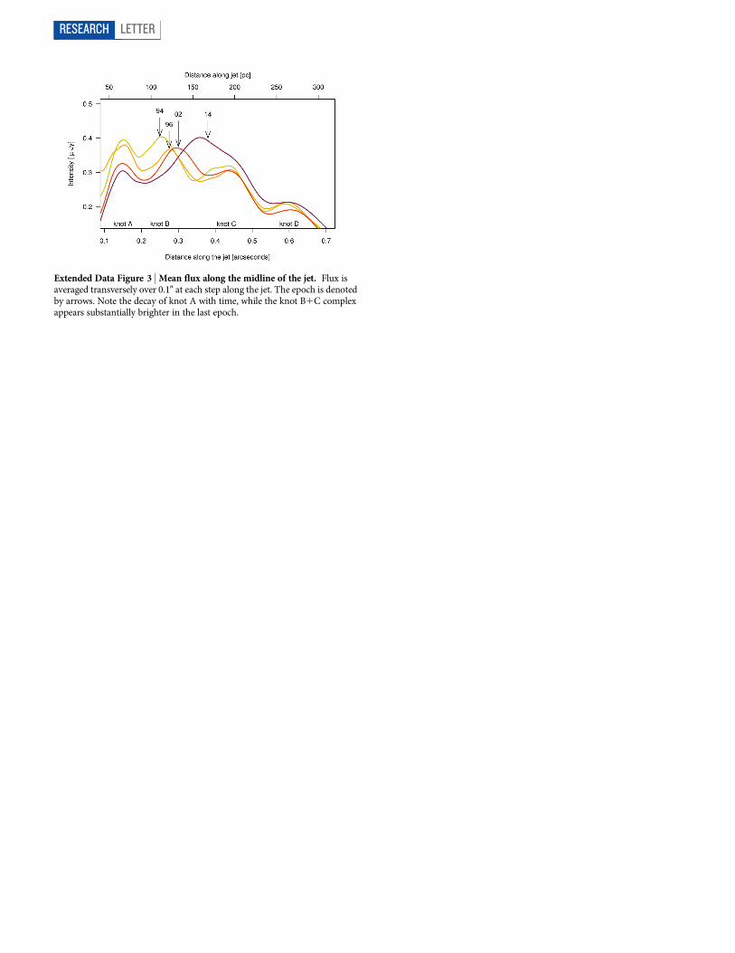
Extended Data Figure 3 | Mean flux along the midline of the jet. Flux isaveraged transversely over 0.10 at each step along the jet. The epoch is denotedby arrows. Note the decay of knot A with time, while the knot B1C complexappears substantially brighter in the last epoch.

RESEARCH LETTER

G2015 Macmillan Publishers Limited. All rights reserved

Extended Data Figure 4 | Comparison of 1983 VLA midline flux to 1994HST midline flux. Flux is averaged transversely over 0.10 at each step along thejet. We fit parabolic forms to the peaks seen in the radio contour to derive roughestimates of knot location, with values depicted with short dashed lines. Dottedlines connecting matched knots are shown to guide the eye.

LETTER RESEARCH

G2015 Macmillan Publishers Limited. All rights reserved

Extended Data Figure 5 | Comparison of 1983 radio positions of knots withHST data. The locations of knots B and C in 1983 are denoted by triangles, andwe include an estimated 15 mas error on the position based on a typicalcentroiding error of 10% of the beam size (0.150). Optical data are identical tothat described in Fig. 2. For knot C, a dashed line gives the fit to epochs 1983 and1994. For knot B, the dashed line is a parabolic fit to all data. The location ofknot A is noted with a dotted line.

RESEARCH LETTER

G2015 Macmillan Publishers Limited. All rights reserved

Extended Data Figure 6 | Depiction of background subtraction method.a, The final 2014 image stack before subtraction. b, The mask used in modellingthe galaxy and dust disk. (White areas were not used in fits.) c, The final 2014

galaxy and dust model. d, The same image as a after c has been subtracted.Physical scaling of all images and flux scaling of a, b and d are identical.

LETTER RESEARCH

G2015 Macmillan Publishers Limited. All rights reserved

Extended Data Figure 7 | Depiction of modelling results. a, The resulting background-subtracted model image for the 2002 epoch. b, The real background-subtracted 2002 image. In both cases the image box is shown by the red outline. Only pixels within this area were used in the fit.

RESEARCH LETTER

G2015 Macmillan Publishers Limited. All rights reserved

Extended Data Table 1 | Maximum-likelihood modelling results

*Systematic error of 3.5 (0.18) mas for WFPC2 (ACS) images has been added to the measurement error from column 3. {Knot A values are included for completeness; see Methods for note on reliability of knot Apositions.

LETTER RESEARCH

G2015 Macmillan Publishers Limited. All rights reserved