UBRARY

NAVAi POSTGRAOUArf SCHCKH MONTEREY CALIFORNIA 93943

Naval Ocean Research and ''Development Activity -

NSTL, Mississippi 39529

NORDA Technical Note 301

A Laser Slope Gauge and a Spar Buoy Wave Gauge: /u>* Mo& Tools for the Validation of Microwave Remote Sensors

Approved for Public Release Distribution Unlimited

P. M. Smith C. S. Lin Ocean Sensing and Prediction Division Ocean Science Directorate

December 1984

ftv-B W^

ABSTRACT

Two devices designed to measure high frequency wave amplitude and slope are described: a spar buoy capacitance wave probe and a laser slope gauge. The spar buoy was equipped with a conventional capacitance wire probe while being tethered to a ship in coastal waters. The buoy demonstrated the capability for measuring wave height spectra at frequencies up to 2.5 Hz. The buoy hull responded weakly to the gravity wave field due to a resonant period of 7 seconds. With proper design modifi- cations this buoy could operate independently of a tether, in deep waters, and with a frequency response up to 20 Hz. The laser slope gauge was designed to operate in water less than 1.3 m in depth. The gauge was equipped with a solid state, UDT X-Y position detector. The detector demonstrated exceptional frequency response (>1 kHz) and high spatial resolution. Wind-wave slope data obtained using this instrument reveal the ubiquitous nature of parasitic capillary waves.

ACKNOWLEDGMENTS

The laser slope gauge work was supported by Program Element 61153N under the sponsorship of Dr. J. E. Andrews of NORDA. The spar buoy wave probe was supported by Program Element 62759N under the sponsorship of CAPT J. Ford of NAVAIRSYSCOM. The technical assistance of Mr. Dan Olive of the Computer Sciences Corporation Electronics Engineering Lab is gratefully acknowledged. Dr. M. Y. Su made available the outdoor wave facility for the testing of the laser probe.

ii

CONTENTS

INTRODUCTION 1

SPAR BUOY-MOUNTED CAPACITANCE WAVE PROBE 1

LASER SLOPE GAUGE 6

THE DETECTOR 10

THEORY 14

SAMPLE TIME SERIES 17

CONCLUSIONS 21

REFERENCES 21

ILLUSTRATIONS

Figure 1. Notation for wave buoy relative to sea surface 2

Figures 2a and 2b. Buoy transfer function 4

Figure 3. Schematic of wave buoy 5

Figure 4. Spectra taken over Nantucket Shoals 7

Figure 5. Uncompensated spectra vs. conpensated spectra 8

Figure 6. Schematic drawing of laser instrument 9

Figure 7. Photograph of laser slope gauge 11

Figure 8. Photograph of laser slope gauge 12

Figure 9. Detector face-scanning pattern 13

14

Figure 11. Schematic drawing of refracted beam at air-water interface 17

Figure 12. Schematic of beam focusing on diffuser 19

Figure 13. Time series of laser output voltages: wind waves 20

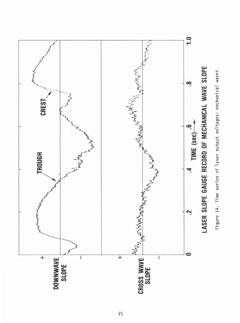
Figure 14. Time series of laser output voltages: mechanical waves 21

TABLE

Table I. Mapping function coefficients 16

Figure 10. 3-D plot of Vx2 + Vy

2 surface vs. X and Y

in

A LASER SLOPE GAUGE AND A SPAR BUOY WAVE GAUGE

INTRODUCTION

We describe two instruments which have proven useful for in situ measurements of surface waves at high frequencies: a spar buoy capacitance gauge for wave eleva- tion and a laser slope gauge for wave slope. The former instrument has been deployed in coastal waters, tethered from a ship, whereas the laser has been employed in a shallow, enclosed, fresh water basin. The spar buoy data was sampled at 5 Hz to provide an upper frequency spectral cutoff of 2.5 Hz. With some design modifications the buoy could be deployed in the deep ocean and the frequency extended to 20 Hz. The buoy, then, would be capable of providing in situ data suitable for the modeling of microwave scattering from the sea surface for L- and C-Band microwave instru- ments. The laser instrument, while not deployable at sea as presently configured, exhibits a very high frequency response (>1 kHz). Slope measurements of 3 to 6 mm waves become possible with this instrument, allowing in situ surface truth for microwave frequencies up to Ka Band. Both of these instruments fill a critical need for in situ measurement techniques for the analysis of short, high frequency waves.

SPAR BUOY-MOUNTED CAPACITANCE WAVE PROBE

The spar buoy has attracted the interest of engineers and scientists for a number of years because of its stability as an instrument platform. Since the response of the spar buoy to waves can be made quite small at typical ocean wave frequencies (f>0.1 Hz), it makes an ideal platform for mounting wave gauges, meteor- ological sensors, and acoustic transponders. The majority of spar buoys in use today are used for basic research. The most famous example is FLIP (Floating Instrument Platform), which was built and operated by the Scripps Institution of Oceanography. FLIP has a resonant period of about 25 seconds (Kerr, 1964), making it relatively insensitive to the spectrum of oceanic gravity waves. A need for fine-scale, high-frequency wave measurements has come with the advent of satellite microwave sensors—coherent radars, scatterometers, and radiometers. Heave buoys and direc- tional wave slope buoys do a good job of estimating the energetic portion (f<0.9 Hz) of the wave spectrum, but centimeter scale wave measurements are needed to explain the areal and temporal variations in the microwave scattering properties of the sea surface. The spar buoy equipped with a capacitance probe (or resistance probe) could answer that need. But first I will review the theory of the motion of a spar buoy. Utilizing the notation of Figure 1, the spar buoy displacement, plus the relative displacement of the sea surface as measured by an attached capacitance probe, gives the true free surface displacement:

x + v = y (1)

From Berteaux (1976), the equation of motion for a spar buoy, forced by a sinusoidal wave of wavenumber, k, is:

ex + bx + mv x = (cy + by + m'y) e'kD (2)

where c = pAg

A = cross-sectional area

b = damping coefficient

DATUM

WATER LINE

Figure 1. Notation for wave buoy relative to sea surface

m (virtual mass of buoy) = m + m' m = mass of the buoy m' = mass of the entrained water D = depth of the buoyant section below the water line

Also,co0 (resonant frequency of the unforced buoy) p Ag mv J

(3)

Upon eliminating x from (2) by substitution from (1) we get:

c (l-e"kD) y + b (l-e"kD) y + (my - m'e"kD) y = en + bi? + myrj (4)

Applying the Fourier Transform operator to Equation (4) and grouping terms gives:

c - co m + i co b Y(co) = JL H(co) (5)

where

S = (1 - e-w2[)/9) - co2(mv - niV"2^) + icobd - e^0^),

and Y and H are the transforms of y(t) and v[t), respectively. The power spectrum of wave elevation, as measured by the buoy, can then be corrected for the buoy motion by multiplying the spectrum by the modulus of the transfer function squared:

Y(co)2 = T(w)2 * H(w)2 (6)

Figures 2a and 2b show T(co) for the NORDA spar buoy.

A schematic of the wave gauge buoy is shown in Figure 3. The resonant frequency of the buoy as measured in a test tank is about 7 seconds, and the virtual mass of the buoy is approximately 45 kgm. Since the actual mass of the buoy was measured to be only 6 kgm, the damper plate is responsible for an additional 39 kgm of entrained water. The buoy was designed to be tethered from a ship with the data being digit- ized and logged on board. The buoy hull is a 4 cm diameter by 3.3 meters long fiber- glass tube with a water-tight compartment occupying the upper 1.4 meters. The damper plate is 0.5 meter in diameter. The buoy is fitted with a vane to keep the capaci- tance probe into the wind. The capacitance probe electronics (McGoldrick, 1971) are housed in the water-tight, upper compartment of the buoy, and a grounding wire is led out to a ground plate to form the ground side of the capacitor. The probe itself is 0.4 mm varnished magnet wire and is attached to the lower stand-off by a tension- ing spring. A resistance wire of like diameter has been shown to have a frequency response of up to 20 Hz (Liu & Lin, 1982). Since the buoy is light and easy to handle it is well suited to the task of obtaining high-frequency wave spectra for short intervals of time at many stations.

The buoy was deployed from an 85-foot vessel at several stations over the Nantucket Shoals in support of simultaneous airborne microwave measurements. Two examples of power spectra taken on different days, under different wind conditions,

SPAR BUOY TRANSFER FUNCTION

(a)

(b)

T(»)

-1

-2

-3

^ *R L

-zs- | i i ,

— __— ,

T.

10

.5 .7 1.0 2.0 FREQUENCY (CYCLES/SEC) •

5.0

2 1 — PERIOD (SEC)

MODULUS SQUARED OF BUOY TRANSFER FUNCTION

.2 .3 .5 .7 1.0

FREQUENCY (CYCLES/SEC)-

10 -i r

2 1 — T (SEC)

—r~ .5

Figures 2a and 2b. Buoy transfer function

ELECTRONICS

PLEXIGLASS VANE

GROUND PLATE

POLYURETHANE FOAM

DAMPER PLATE^

INSULATED WIRE

WATERTIGHT COMPARTMENT

-TO SHIP SIGNAL CARLE

LEAD WEIGHTS

U OVERALL LENGTH - 3.1 METERS

WEIGHT - 6 KGM

WIRE LENGTH - 1.2 METERS

Figure 3. Schematic of wave buoy

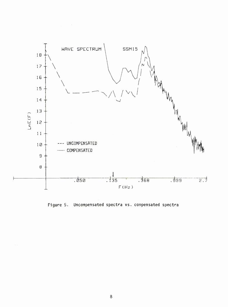
are shown in Figures 4a and 4b. Both spectra exhibit the Phillips equilibrium spec- tral roll-off of f"5'(Phillips, 1982). The spectrum of Figure 4a was obtained under relatively light wind conditions and exhibits a spectral peak somewhat displaced downward in frequency from the equilibrium wind-wave field. The second spectrum was obtained under stronger wind conditions and is dominated by wind waves. The records were 10 minutes long, sampled at 5 Hz, and were band averaged to achieve 30 degrees of freedom. The confidence limits shown by the brackets are at 95%. Figure 5 demon- strates the effect of compensation for the buoy motion on one of the measured wave spectra. The error due to buoy motion does not appear to be appreciable above about 0.9 Hz. Since these data were obtained over shoals where the wave field loses its energy to breaking, the spectral peak was at a relatively high frequency and buoy motion did not unduly distort the measured spectrum. In the deep ocean under the influence of swell, however, the buoy should be designed to have a longer resonant period. Calculations based on drag formulae, published in Berteaux (1976), indicate that merely doubling the size of the damper to 1 meter in diameter should increase the resonant period to 12 seconds.

LASER SLOPE GAUGE

The laser slope gauge is a device primarily intended to measure the slopes of high-frequency (f>l Hz) surface gravity and capillary waves. Early small-wave measurements used incoherent light as a probe (Cox, 1958) and resulted in the first estimation of the capillary wave spectrum. The introduction of the laser and suitable laser detectors encouraged more investigators to probe the response of the centimeter-scale waves to wind and mechanical waves in laboratory tanks (Long and Huang, 1976; Bobb et al., 1979; Liu and Lin, 1982). Field deployments of laser slope gauges are relatively rare. Tang and Shemdin (1983) deployed a tower-mounted laser "Wave-Follower" during the MARSEN experiment in 1979. Hughes and Gower (1983) and Hughes (1978) deployed a laser slope gauge from the bowsprit of a moving vessel for the analysis of internal wave modulations. The advantages of the laser slope gauge wave probe are: 1) the instrument does not interfere with the phenomena being measured, 2) the frequency response of the detectors is high enough to span the entire capillary spectrum, and 3) the small (typically 1 mm) beam spot size makes high spatial resolution measurements possible.

The slope gauge reported here was designed to rest on the bottom of a shallow, fresh water basin. The laser section is submerged and the refracted beam is col- lected and sensed by an optics assembly installed above the water. A schematic of the instrument is shown in Figure 6. The optics design follows that described by Tober et al . (1973). The laser, a 10 mW He-Ne Hughes Model 3235H-PC, is encased in a watertight enclosure at the bottom. The enclosure window is a double convex lens having a focal length of 30 cm. This lens focuses the laser beam to a 1 mm spot size at the air-water interface. The beam is deflected vertically by a front-surface mirror and is deflected away from the local normal on passing through the air-water interface. The beam is then focused on to the diffuser plate by the collimating lens. This lens is a 145 mm diameter plano-convex lens having a focal length of 450 mm. The collimating lens is the heart of the optics system, mapping the refracted beam angle to a displacement on the diffuser plate. Thus, any beam leaving the air-water interface at a given angle will map to the same point on the diffuser regardless of the vertical displacement of the interface. The diffuser is a 1/4 inch glass plate with a finely ground upper surface. A detector lens is located above the diffuser and focuses the diffuser image onto the face of the detector. This lens is a 60 mm diameter, 100 mm focal length plano-convex lens.

-12

WAVE SPECTRUM RUN 13; STATION 12; 6:

1 .05

20

.14 .37 f(Hz)

—i 1— 7.4 2.7

T(sec)

1.0

-1— 1.0

2.5

—I 0.4

-2

-4

ui - 6 -

10

-12 .05

20

WAVE SPECTRUM RUN 16; 55 M16; 22.5;

.14

• (Hz)

.37 1.0 2.5

7.4

T(sec)

I 2.7

I 1.0

1 fl.4

Figure 4. Spectra taken over Nantucket Shoals

\ WRVE SPECTRUM 18 -

"\

1? - \

1G -

15 -

\

\

14 -

Ld C

13 -

12 -

1 1 -

10- — UNCOMPENSATED

COMPENSATED 9 -

i

8 -

i 1 .050 "I" 3 5 7^ G8 199 2 . r'

FCHz)

Figure 5. Uncompensated spectra vs. conpensated spectra

X - Y POSITION DETECTOR

COLLECTING OPTICS

GLASS DIFFUSER

VslATERsc^ COLLIMATING LENS

APERTURE

WATER-TIGHT ENCLOSURE „

LASER ft

Normal to Surface

^MIRROR

u

Figure 6. Schematic drawing of laser instrument

The slope dynamic range of the instrument is determined by the size of the col- limating lens and the proximity of this lens to the mean water surface. For example, if the 15 cm lens is located 15 cm from the water surface the dynamic range will be +45 degrees. The range is inversely related to the lens-interface distance. Doubling that distance will halve the dynamic range. Wave crests will exhibit a larger dynamic range than the troughs because they are closer to the collimating lens. An ocean deployment of this type of instrument requires some kind of wave follower (Tang and Shemdin, 1983) in order to retain the dynamic range and to keep the instrument from swamping. Figures 7 and 8 are photographs of the instrument.

THE DETECTOR

The detector is a United Detector Technology Model SC-50 X-Y position detector having an active area of approximately 4 cm by 4 cm. The detector, together with its associated signal analyzer/amplifier (UDT Model 331), senses the X and Y position of the laser spot on the diffuser and produces two analog voltages that are proportion- al to the two components of displacement. The detector material is composed of two layers of planar diffused Schottky Barrier type PIN diodes. The advertized frequency response is 5 kHz. We operated it at 1 kHz with satisfactory results.

Another type of detector used for this purpose is that of Hughes and Gower (1983). Their detector is a scanned array of discrete diodes (EG&G Reticon Model RA100). The array is scanned at 400 Hz with a spatial resolution of 100 elements. This type of device does not have the spatial resolution or the frequency response of the UDT device but the discrete diode array exhibits a higher sensitivity to light and retrieval of position data is much easier.

The UDT detector position information is sensitive to fluctuations in light intensity. The effects of short term intensity fluctuations are automatically removed in the amplifier electronics. Longer term lighting changes are compensated for by manually changing the amplifier gain and bias.

Ideally, the X displacement of the laser spot on the UDT detector surface should be proportional to V„ and the Y displacement proportional to VY, where Vy and

Vy are the two output voltages present at the amplifier output terminals. The

response, however, is not perfectly linear, and there is some cross-coupling between axes. The mapping of the set, JX, Yf to the the set, |Vw, Vy[, must then be deter- mined. In order to determine the mapping functions:

and

X = f(Vx, Vy) (7)

Y = g(Vx, Vy) (8)

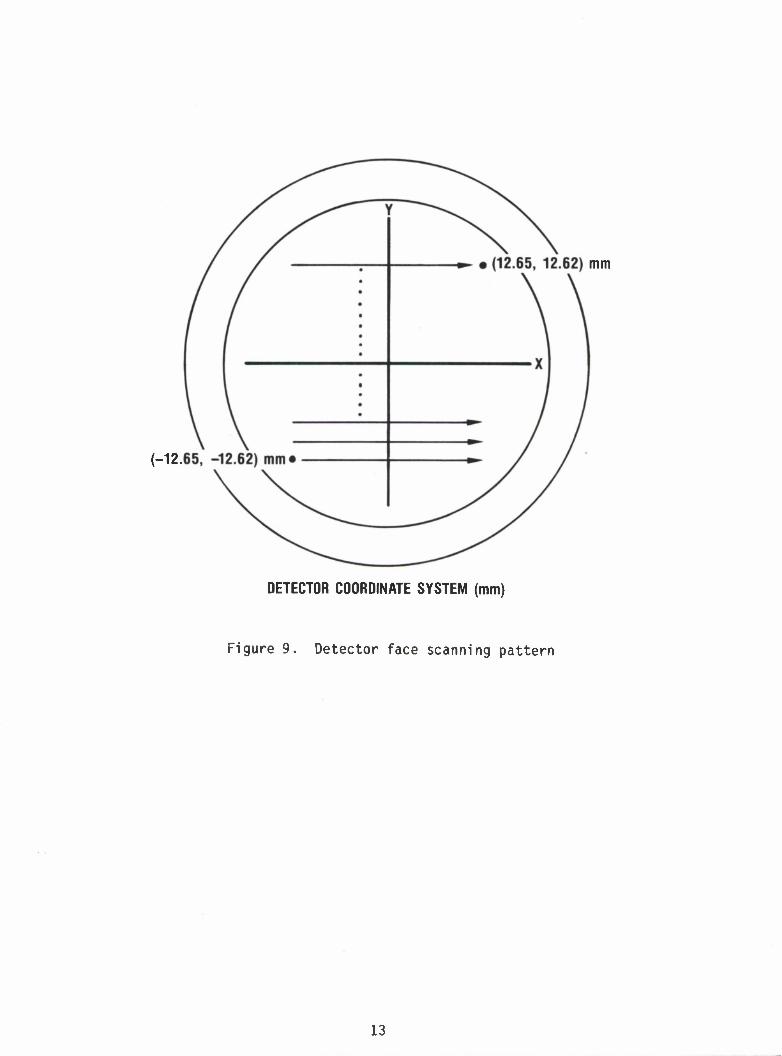
for the UDT detector and amplifier, stepping motors were installed near the top of the instrument to control the detector stage. The laser beam was held fixed and the

detector stage was scanned across the beam in discrete steps. Vx and vy were meas"

ured at each step, defining a 41 X 41 array (see Fig. 9). The surface defined by the 7 ?

function, Vw + Vy, obtained from one such scan, is shown plotted against X and Y in

Figure 10. If Vy and VY are linear functions of X and Y, respectively, the surface

10

Figure 7. Photograph of a laser slope gauge (a). The same photograph enlarged and with the background removed (b).

11

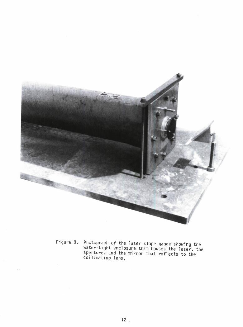
Figure 8. Photograph of the laser slope gauge showing the water-tight enclosure that houses the laser, the aperture, and the mirror that reflects to the collimating lens.

12

(-12.

mm

DETECTOR COORDINATE SYSTEM (mm)

Figure 9. Detector face scanning pattern

13

-o c <0

>

O <o 4- S-

CM >-

CM

O

Q I

CO

CD

14

6 • L

i=0

6-1

j=o

6

1=0

6-1 £ j-o

should describe a cone. Figure 10 reveals that linearity is good except near the edges where the surface begins to roll over. In order to obtain expressions for equations (7) and (8) the data was fit to sixth order bivariate polynomials in the least squares sense. The polynomial equations can be written thus:

A1j vx vy <9'

B,j VJ VJ (10)

Table I lists the resulting coefficients. V„ and Vy are in millivolts and X and Y

are in arbitrary array coordinates. Since A.Q >> AQ. and BQ. >> B,Q, the detectors

operate approximately as advertised. However, A.., B,., and most higher order

coefficients taken to the appropriate root each represent about 10% of the coefficient of the linear term. Hence, a linear mapping is not sufficient for the retrieval of X and Y. Tests to recover the original positions from Equations (9) and (10) show a retrieval accuracy of about 0.3%.

As mentioned above, the ambient lighting conditions together with the varia- tions in the intensity of the laser light (which is affected by water clarity) can affect the offset and gain of the detector amplifier. The long term solution to this problem is to lead out the four preamp outputs for data logging and perform the removal of the intensity effects in the computer. In this way gain and offset changes can be tracked and calibration can be maintained.

THEORY

The laser beam is refracted away from the local normal and toward the vertical as it passes through the air-water interface. The angle of the beam relative to the local normal, 0., obeys Snell's Law:

n1 Sin01 = n2 Sin92- (11)

9j = Sin" [n2/n1 SinOg]

= Sin"1 [1.332 Sin02]

for fresh water, where n refers to the index of refraction and the angles are defined as in Figure 11. 0, the angle between the beam and the vertical can now be obtained in terms of the slope angle, 92:

0 = 91 - 92

= Sin-1 [1.332 Sin92] - 92- (12)

For 9 < 10°, 9 = Sin9 +0(0.001). For 0 < 20°, 9 = SinO +0(0.007).

so that, for 92 < 20°, 0 = 0.33292-

15

TABLE 1. MAPPING FUNCTION COEFFICIENTS

Term Au B..

1J

vovo VY -2.9 -1.5

VX 3.7 X 10"2 -0.32 X 10'2

VY 0.03 X 10"2 -3.4 X 10"2

V2 0.5 X 10"5 -2.0 X 10"5

V V yXVY 0.11 X 10'5 -1.2 X 10"5

V2 VY 0.52 X 10"5 1.0 X 10'5

V3 VX 0.17 X 10"9 -3.4 X 10"9

2 V V VXVY 7.4 X 10"9 21 X 10"9

V V VXVY -9.8 X 10'9 19 X 10"9

V3 8.6 X 10"9 -25 X 10"9

V4 VX -6.2 X 10"11 22 X 10"11

vx\ -5.0 X 10"11 -3.7 X 10"11

v2v2 VXVY -2.7 X 10"11 5.3 X 10"11

V V VY 2.4 X 10"11 5.0 X 10"11

Term *u B.. 1J

v4 VY -1.8 X 10"11 -4.1 X 10"11

V5 vx 13 X 10"14 3.0 X 10"14

V4VY -2.7 X 10"14 2.0 X 10"14

3 2 V V VY -7.7 X 10"14 0.95 X 10"14

VXVY -6.0 X 10"14 8.1 X 10"14

4 VXVY 0.68 X 10'14 -5.1 X 10"14

v5 VY -6.6 X 10"14 -6.2 X 10"14

V6 0.04 X 10"16 -9.5 X 10"16

5 V V VXVY 0.72 X 10"16 -5.8 X 10"16

4 2 V V VXVY 3.3 X 10'16 0.33 X 10"16

3 3 VXVY -2.4 X 10"16 2.2 X 10~16

V2V4 VXVY 0.59 X 10"16 0.99 X 10"16

5 V? 1.1 X 10"16 0.84 X 10"16

v6 VY 2.1 X 10"16 1.3 X 10"16

16

REGION 1

REGION 2

Figure 11. Schematic drawing of refracted beam at air-water interface

17

In accordance with Figure 12, the displacement, d, of the beam on the diffuser is linearly related to Tan0:

d(mm) = 450 Tan0.

After substitution from Equation (12),

d(mm) = 450 Tan [Sin-1 (1.33202) - 02]. (13)

For 02 < 20°,

d(mm) a 14992

where 92 is approximately equal to the slope (Tan 02). The recorded values of Vx and

Vw should, then, be approximately linearly proportional to the slope components, L

and lw, for slope angles less than 20°, if we ignore nonlinearities introduced by

the detector and use the small angle approximation.

SAMPLE TIME SERIES

Slope data for wind waves and mechanical waves were collected at an outdoor basin measuring 30 cm deep by 100 m by 300 m. The facility is described in Su (1982). Due to biological activity in the water, severe attenuation of the laser beam was experienced under zero wind speed conditions. The resulting low levels of light intensity required that data be collected at night since the detector could not discriminate between the laser image and the ambient light fluctuations. The insertion of a band-pass filter did not alleviate the problem. However, when the wind speed increased to about 5 m/sec the activities of the organisms ceased and water clarity improved markedly. Under these conditions there was a marked increase in signal from the detector. We did not attempt to make daytime measurements under these conditions and, hence, we cannot comment on the operation of the UDT detector under daylight conditions when the water column is clear.

The wind fetch during the collection of wind wave data was approximately 300 m and the wind speed was estimated to be about 5 m/sec. Figure 13 shows a sample time series from this data set. Cross-wind and down-wind voltages, Vw and VY, are

shown as functions of time. Since the wave crests are characterized by small radii of curvature relative to the troughs, the crests display rapidly rising signatures while the troughs exhibit a gradually dropping signature. Note the well-defined capillary wave trains preceding some of the crests. These waves were first noticed by Cox (1958) and were later explained by Longuet-Higgins (1963). These waves are postulated to be stationary relative to a reference frame moving with the phase speed of the primary gravity wave. The frequency of the first wave train (marked "A" in the figure) is observed to be approximately 100 Hz whereas the frequency of the second wave train (marked "B" in the figure) is approximately 200 Hz. The phase speed of the larger gravity wave was estimated to be 60 cm/sec which would imply that the wavelengths of the capillaries were 6 mm and 3mm, respectively.

Figure 14 shows a time series of slopes derived from a mechanically generated wave propogating in the same wave basin under near-zero velocity wind conditions. The slope gauge is positioned about 10 meters from the wave generator. While the large scale mechanical wave dominates the slope time series, a small amplitude, fine

18

d H

Figure 12. Schematic of beam focusing on diffuser

19

to

>

C3

CO LU Q_ o -o

c

00 •r— 5

UJ > to ^£ a>

£ a o .^ > -f £ 4->

1 u_ Q.

o C3 13 CD o 00 £^

*""* oc s-

UJ o <1J to

^ o m UJ r—

I— cc t|-

UJ O

rr CD to

< s- C9 a;

to

CO

0)

CO

00 a> CM <

en " —1 •r— u_

+ +

CO CO

CO I*:

20

to CD >

*3

o

to <D cn n3 4->

o >

ex 4->

0) to

to

1° eo3

21

structure of capillaries rides on the surface. Also an anomalous bump in the slope record rides on the forward slope of each wave. This bump is the precurser of a Benjamin-Feir sideband instability which becomes more fully developed down-wave (Su, 1982).

CONCLUSIONS

The laser slope gauge is a powerful tool for the diagnosis of the shorter gravity-capillary and capillary waves since, unlike the elevation spectrum which

_5 drops off rapidly as f , the slope spectrum drops off at the much slower rate of

f" . The capillary waves, however, do not dominate the slope spectrum, and so the slopes of the larger waves are still evident in the time series. The UDT detector, while lacking in sensitivity, demonstrated its usefulness in recording the very high frequency (f>100 Hz) waves. These small waves must be adequately sampled if their curvature properties are to be determined.

REFERENCES

Berteaux, H. 0. (1976). Buoy Engineering. John Wiley & Sons, 314 pp.

Bobb, L. C, G. Ferguson, and M. Raukin (1979). Capillary Wave Measurements. Applied Optics, v. 18, pp. 1167-1171.

Chang, J. H., W. N. Wagner, and H. C. Yuen (1978). Measurement of High Frequency Capillary Waves on Steep Gravity Waves. Journal of Fluid Mechanics, v. 86, pp. 401-413.

Cox, C. S. (1958). Measurements of Slopes of High Frequency Wind Waves. Journal of Marine Research, v. 16, pp. 199-225.

Hughes, B. A. (1978). The Effect of Internal Waves on Surface Wind Waves. 1. Experimental Measurements. Journal of Geophysical Research, v. 83, pp. 455-465.

Hughes, B. A. and J. F. R. Gower (1983). SAR Imagery and Surface Truth Comparisons of Internal Waves in Georgia Strait, British Columbia, Canada. Journal of Geophysical Research v. 88, pp. 1809-1824.

Kerr, K. P. (1964). Stability Characteristics of Various Buoy Configurations. Transactions of the 1964 Buoy Technology Symposium, pp. 1-16.

Liu, H. and J. Lin (1982). On the Spectra of High Frequency Wind Waves. Journal of Fluid Mechanics, v. 123, pp. 165-185.

Long, S. R. and N. E. Huang (????). Observations of Wind-Generated Waves on Variable Current. Journal of Physical Oceanography, v. 6, pp. 962-968.

Longuet-Higgins, M. S. (1963). The Generation of Capillary Waves by Steep Gravity Waves. Journal of Fluid Mechanics, v. 16, pp. 138-159.

McGoldrick, L. F. (1971). A Sensitive Linear Capacitance-to-Voltage Converter, with Applications to Surface Wave Measurements. Review of Scientific Instruments, v. 42, pp. 359-361.

22

Phillips, 0. M. (1982). The Dynamics of the Upper Ocean. 2nd ed., Cambridge University Press, New York.

Su, M. (1982). Three-Dimensional Deep-Water Waves. Part 1 Experimental Measurement of Skew and Symmetric Wave Patterns. Journal of Fluid Mechanics, v. 124, pp. 73-108.

Tang, S. and 0. H. Shemdin (1983). Measurement of High-Frequency Waves Using a Wave Follower. Journal of Geophysical Research, v. 99, pp. 9832-9840.

Tober, G., R. C. Anderson, and 0. H. Shemdin (1973). Laser Instrument for Detecting Water Ripple Slopes. Applied Optics, v. 12, pp. 788-794.

23

UNCLASSIFIED SECURITY CLASSIFICATION OF THIS PAGE

REPORT DOCUMENTATION PAGE

1a REPORT SECURITY CLASSIFICATION

Unclassified 1b RESTRICTIVE MARKINGS

None 2a SECURITY CLASSIFICATION AUTHORITY 3 DISTRIBUTION AVAILABILITY OF REPORT

2b DECLASSIFICATION DOWNGRADING SCHEDULE Approved for public release; distribution is unlimited.

4 PERFORMING ORGANIZATION REPORT NUMBER(S)

NORDA Technical Note 301

5 MONITORING ORGANIZATION REPORT NUMBER(S)

NORDA Technical Note 301

6 NAME OF PERFORMING ORGANIZATION

Naval Ocean Research and Development Activity

7a NAME OF MONITORING ORGANIZATION

Naval Ocean Research and Development Activity

6c ADDRESS (City. Stale, and ZIP Code)

Ocean Science Directorate NSTL, Mississippi 39529

7b ADDRESS (City. State, and ZIP Code)

Ocean Science Directorate NSTL, Mississippi 39529

8a NAME OF FUNDING SPONSORING ORGANIZATION

Naval Ocean Research and Development Activity

8b OFFICE SYMBOL (It applicable)

9 PROCUREMENT INSTRUMENT IDENTIFICATION NUMBER

8c ADDRESS (City. State, and ZIP Code)

Ocean Science Directorate NSTL, MS 39529

10 SOURCE OF FUNDING NOS

PROGRAM ELEMENT NO

61153N

PROJECT NO

TASK NO

WORK UNIT NO

1 1 TITLE (Include Security Classification)

A Laser Slope Gauge and a Spar Buoy Wave Gauge: Tools for the Validation of Microwave Remote Sensors 12 PERSONAL AUTHOR(S)

P. M. Smith and C. S. Lin 13a TYPE OF REPORT

Final 13b. TIME COVERED

From To

14 DATE OF REPORT (Yr , Mo . Day)

December 1984 15 PAGE COUNT

24 16 SUPPLEMENTARY NOTATION

COSATI CODES 18 SUBJECT TERMS (Continue on reverese if necessary and identify by block number)

Wave amplitude, wave slope, spar buoy, slope gauge

19 ABSTRACT (Continue on reverse if necessary and identify by block number)

Two devices designed to measure high frequency wave amplitude and slope are described: a spar buoy capacitance wave probe and a laser slope gauge. The spar buoy was equipped with a conventional capacitance wire probe while being tethered to a ship in coastal waters. The buoy demonstrated the capabili- ty for measuring wave height spectra at frequencies up to 2.5 Hz. The buoy hull responded weakly to the gravity wave field due to a resonant period of 7 seconds. With proper design modifications this buoy could operate independently of a tether, in deep waters, and with a frequency response up to 20 Hz. The laser slope gauge was designed to operate in water less than 1.3 m in depth. The gauge was equipped with a solid state, UDT X-Y position detector. The detector demonstrated exceptional frequency response (> 1 kHz) and high spatial resolution. Wind-wave slope data obtained using this instrument reveal the ubi- quitous nature of parasitic capillary waves.

20 DISTRIBUTION AVAILABILITY OF ABSTRACT

UNCLASSIFIED, UNLIMITED D SAME AS RPT. DTIC USERS I J

21 ABSTRACT SECURITY CLASSIFICATION

Unclassified 22a NAME OF RESPONSIBLE INDIVIDUAL

P. M. Smith

22b. TELEPHONE NUMBER (Include Area Code)

(601) 688-5267

22c OFFICE SYMBOL

Code 321

DD FORM 1473, 83 APR EDITION OF 1 JAN 73 IS OBSOLETE UNCLASSIFIED SECURITY CLASSIFICATION OF THIS PAGE