a leg proprioception based 6 dof odometry for statically...

Autonomous Robots Journal manuscript No.(will be inserted by the editor)

A Leg Proprioception Based 6 DOF Odometry for StaticallyStable Walking Robotshttp://link.springer.com/article/10.1007/s10514-013-9326-3

Martin Gorner · Annett Stelzer

Received: date / Accepted: date

Abstract This article presents a 3D odometry algo-rithm for statically stable walking robots that only usesproprioceptive data delivered by joint angle and joint

torque sensors embedded within the legs. The algorithmintrinsically handles each kind of emerging staticallystable gait and is independent of predefined gait pat-

terns. Additionally, the algorithm can be equally ap-plied to stiff robots as well as to robots with compli-ant joints. Based on the proprioceptive information a 6

degrees of freedom (DOF) pose estimate is calculatedin three steps. First, point clouds, represented by thefoot positions with respect to the body frame at two

consecutive time steps, are matched and provide a 6DOF estimate for the relative body motion. The ob-tained relative motion estimates are summed up over

time giving a 6 DOF pose estimate with respect to thestart frame. Second, joint torque measurement basedpitch and roll angle estimates are determined. Finally

in a third step, these estimates are used to stabilize theorientation angles calculated in the first step by datafusion employing an error state Kalman filter. The algo-

rithm is implemented and tested on the DLR Crawler,an actively compliant six-legged walking robot. For thisspecific robot, experimental data is provided and the

performance is evaluated in flat terrain and on gravel, atdifferent joint stiffness settings and for various emerginggaits. Based on this data, problems associated with theodometry of statically stable walking robots are iden-

tified and discussed. Further, some results for crossingslopes and edges in a complete 3D scenario are pre-sented.

Martin Gorner · Annett StelzerRobotics and Mechatronics Center, German Aerospace Cen-ter (DLR e.V.), 82234 Wessling, GermanyE-mail: [email protected]

1 Introduction

As the technology progresses, heterogeneous groups ofmobile robots operating at different levels of autonomywill be deployed in future terrestrial search and res-

cue missions as well as extra-terrestrial planetary ex-ploration scenarios. Within these groups, legged robotswith their high mobility and intrinsic manipulation ca-

pability are very well suited to serve as the rough ter-rain specialists for short range tasks. Their areas of op-eration involve environments such as debris cluttered

urban terrain, natural and artificial caves, craters andcanyons. To fulfill their tasks, the robots must be able tonavigate autonomously. Usually, for the anticipated sce-

narios, no or incomplete a priori information, like mapsor known landmarks, is available. Further, absolute ref-erence as provided by GPS or an external magnetic

field might be unavailable or extremely noisy. Thus, therobots cannot rely on these and must be able to acquireall necessary information about their state and their en-

vironment by themselves. For this purpose the robotsmust use all available data provided by their onboardsensors to the maximum extent. Since a robust pose

estimate is crucial for autonomous navigation withoutreliable external reference, the robots need to optimallycombine different means of ego-motion estimation. Of-

ten, inertial measurement unit (IMU) data and visualodometry are fused to provide these motion estimates.Using dead reckoning, i.e. the summation of motion in-

crements over time, the robots keep track of their 6degrees of freedom (DOF) poses with respect to a localframe. Usually, IMU position estimates are subject to

strong drift and visual odometry is strongly dependenton the visual conditions. Thus, a 6 DOF leg odome-try is a very useful additional source of information to

enhance the robustness of the overall pose estimate.

In this article, we present such a leg odometry algo-

rithm for statically stable walking robots, which in mostcases are four-, six- or eight-legged. The algorithm pro-vides a complete 6 DOF pose estimate which is solely

based on proprioceptive joint angle and joint torquesensors embedded within the legs. This pose estimateis calculated by a three stage algorithm in order to ex-

ploit all the information delivered by the joint sensors.Herein, the first stage provides a 6 DOF relative motionestimate of the robot based on the kinematic configu-

rations of its feet at two consecutive time steps. Sum-ming up the relative motion increments results in a 6DOF pose estimate with respect to a local start frame.

Since this estimate is subject to a drift of the orien-tation angles, the second stage of the algorithm deter-mines absolute pitch and roll angle estimates based on

joint torque measurements. These absolute angle esti-mates are fused in the third stage with the pitch androll angles of the first stage using an error state Kalmanfilter. Thus, only using the proprioceptive sensors em-

bedded within the legs, a complete 6 DOF “pose sen-sor” is obtained that is independent of any IMU or ex-teroceptive sensor. The use of joint torque based pitch

and roll angle estimates is usually not the first choicesince most walking robots provide IMU based orienta-tion data. Nevertheless, our intention is to present and

analyze an alternative method that is based on leg sen-sors only and thus provides redundancy and robustnesswith respect to possible IMU failure. The presented al-

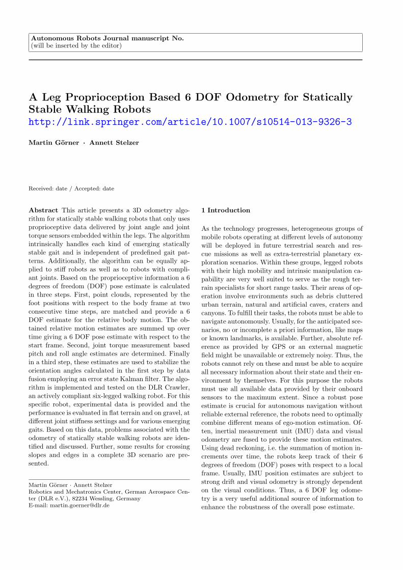
gorithm is implemented and tested on a specific plat-form, the actively compliant, six-legged DLR Crawlershown in Fig. 1. As is true for all methods based on

relative measurements, each leg odometry remains sub-ject to some drift and thus is only useful within certaintemporal and spatial bounds. Nevertheless, as robust

pose estimation in real world navigation scenarios re-quires multiple means of pose measurement, leg odome-try constitutes one possible source. As shown in [1] and

[2], the leg odometry presented in this article is part ofthe visual navigation framework of the DLR Crawler.Herein, leg odometry as well as visual odometry are

aiding sensors in an IMU based fusion scheme for ro-bust pose estimation. The self-contained leg odometryprovides redundancy and strongly enhances the robust-

ness of the navigation in unknown terrain with respectto severe visual disturbances.

The article proceeds as follows. In section 2 we give abrief overview of the related literature. Section 3 intro-

duces the method and presents the three stages of ouralgorithm. In section 4 experimental results are givenfor the DLR Crawler and the effects of different sub-

strates, walking velocities and joint stiffness settings are

Fig. 1 The DLR Crawler within the gravel testbed

evaluated for this specific platform. Finally, we conclude

our work in section 5.

2 Related Literature

In wheeled robotics it is common practice to calcu-

late an odometry based on wheel encoder readings andsteering angles. Usually, wheel odometry returns a pla-nar position as well as the heading angle of the vehicle.

Only very few wheeled robots allow the calculation ofan additional vertical motion estimate based on theirkinematics. One example is the Shrimp robot developed

at EPFL [3]. On this robot an advanced bogie conceptprovides the necessary information for the vertical mo-tion estimate. Nevertheless, the pitch and roll angles,

like on other wheeled robots, have to be estimated byuse of an IMU.

In contrast to their wheeled counterparts, leggedrobots usually provide enough proprioceptive data from

sensors embedded within their legs to calculate a com-plete 6 DOF pose estimate. However, due to the me-chanical complexity, the high number of degrees of free-

dom and the high variety and variability of gaits, theproblem is much harder. Only very few tested leg odom-etry examples returning a full 6 DOF pose are known

to us. Each of those does rely on additional IMU datato either stabilize the results or to compensate for amissing degree of freedom of the pose due to kinematic

constraints. The detailed work on the robot RHex [4,5] is one of the few examples presented in literature.The robot consists of six equal, passively compliant,

single degree of freedom legs and uses its hip joint en-coder readings and leg deformation measurements toestimate its pose. Due to its kinematic configuration

no yaw angle can be calculated by the basic odometryand the data needs to be fused with IMU readings toreturn a full 6 DOF pose estimate. One great advantage

of this approach is that it also covers the flight phases

2

occurring during dynamic running. Another example of

a leg odometry is an algorithm that was developed forthe hexapod Ambler [6] and that was also implementedon the hexapod Lauron [7,8]. In this approach, the sup-

porting legs are used to determine a rigid body trans-formation for the robot with respect to the world frame.The algorithm assumes an ideal no slip ground contact

and finds a minimum error transformation mapping thepositions of the supporting feet at the current time stepwith respect to the body frame onto the stored positions

of the supporting feet with respect to the world frame.After the minimizing transformation is found, the po-sitions of the supporting feet in world coordinates are

recalculated and updated if they changed. This is thecase after a step but should not happen for legs in sup-port according to the ideal no slip condition. In order

to reduce the disturbing effect of slipping legs, individ-ual leg weights are introduced for the transformationcalculation. For Lauron these are obtained by a fuzzyreasoning based contact evaluation. The used leg odom-

etry approach has problems with drifting pitch angleand height estimates. To improve the results the Am-bler odometry discards the tilt angles and replaces them

by inclinometer readings. To achieve improved resultsfor Lauron, its odometry estimates are fused with IMUand magnetic compass based orientation data. As there

is some performance data available for Ambler walkingforward, unfortunately there is no detailed data pub-lished for Lauron. Two recent examples for the use of

leg odometry with dynamic quadrupeds are presentedby [9] and [10]. In the first article Reinstein et al. ob-tain a full pose estimate by fusing a velocity estimate

based on leg odometry with data of an inertial naviga-tion system using an Extended Kalman Filter. In thesecond article, Ma et al. published an approach to im-

prove the navigation robustness of the robot BigDogand its successor project LS3 by multi-sensor data fu-sion using leg odometry [10].

Considering the computation of the relative bodymotion based on the location of the feet, our algorithm

shows similarities to the approaches used for the robotsAmbler and Lauron. The main difference is that ouralgorithm only employs proprioceptive sensors embed-

ded within the legs to obtain a complete 6 DOF poseestimate that incorporates absolute pitch and roll infor-mation. This is achieved by stabilizing the joint angle

based orientation estimates with joint torque measure-ment based absolute pitch and roll angles using an er-ror state Kalman filter. Further, it is important that

our method can be applied to stiff and compliant stat-ically stable walking robots and is able to handle anystatically stable emerging gait. Additionally, we iden-

tify error sources and introduce tuning parameters to

attenuate their effects. Compared to most of the previ-

ous work, the algorithm has been extensively tested andits performance is documented for the DLR Crawlerwalking on different ground substrates, at different joint

stiffness settings as well as at different walking veloci-ties and thus various emerging gait configurations.

3 Method

The basic idea of the presented 6 DOF leg odometryborrows from computer vision. It tries to estimate thechange of the robot pose by finding a minimizing trans-formation between two point clouds which are repre-

sented by the positions of the supporting feet at twoconsecutive time steps. The algorithm requires at leastthree feet in contact and the assumption of rigid point

clouds implies a no slip condition. To reduce errorscaused by drifting orientation angles, absolute pitchand roll angles derived from joint torque measurements

are fused with the joint angle based orientation esti-mates using an error state Kalman filter. Single slippinglegs are detected and in case of a high sampling rate,

the related measurements are discarded without stronginfluence on the pose estimate. Further, the methodcan handle any statically stable emerging gait and can

be adapted to different ground substrates and differ-ent joint stiffness settings by some tuning parametersas documented for the DLR Crawler in section 4. The

use of joint torque sensors for pose estimation seemsto be an additional hardware effort that needs to bejustified. The main reason for using such sensors in

walking robots stems from a control perspective. Jointtorque sensors allow the use of advanced active com-pliance control algorithms with underlying joint torque

control loops and thus support a smooth and robustlocomotion in rough terrain. Several recent examples ofwalking robots exist that employ joint torque sensors

in addition to commonly used joint encoders [11], [12].

3.1 First Stage: Joint Angle Based 6 DOF Pose

Estimate

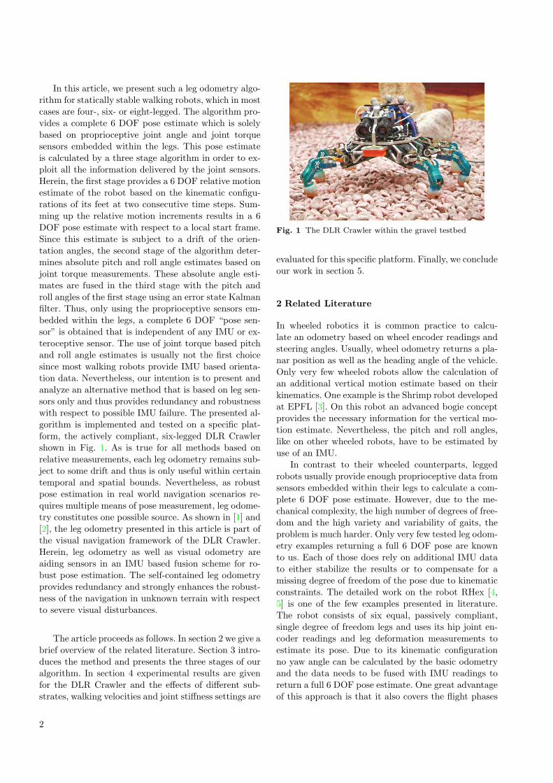
For a statically stable walking robot, as for examplethe DLR Crawler, a change of position and orientationis calculated using two consecutive stance feet config-

urations with respect to the body frame. The result-ing relative motions of the robot body are summedup over time, yielding the pose of the robot with re-

spect to the world frame. Herein, the world frame isbased on the robot body frame at the start positionthat was aligned with the gravity vector along the z-

axis. The body frame is defined as follows. The pos-

3

Fig. 2 Foot contacts and their centroids for two consecutivetime steps with respect to the body frame

itive x-direction points from the back to the front of

the robot and the positive z-direction points upwardsfrom its bottom to its top. The positive y-direction com-pletes a right hand system and the origin is placed at

the center of the robot body. All rotations follow thexyz convention with yaw angle α defined about the z-axis, pitch angle β about the y-axis and roll angle γ

about the x-axis.

In case of the DLR Crawler all calculations are per-formed at the high rate of 1 kHz, which allows discard-

ing single relative motions in case of the detection of ex-cessive slip. For statically stable walking robots, threeor more legs will be in ground contact. Having more

than three feet in stance results in an over-constraintproblem and the odometry needs to account for this.Due to small errors in the kinematics and the rolling

ground contacts of the feet, it is unlikely that the pointclouds perfectly match. Thus, a rigid body transforma-tion with the rotation matrix Rodo and the transla-

tion vector btodo has to be found that minimizes thematching error. The detailed approach to solve thisproblem including the complete derivation was initially

presented in a computer vision paper by Haralick [13].Following, only the necessary equations are given forthe purpose of completeness. The algorithm aims to

minimize ϵ, which is the sum of squared errors of therigid body transformation augmented by constraintsf(λ,Rodo) that enforce an orthogonal rotation matrix,

RodoRTodo = I.

ϵ =n∑

i=1

wi(∥bpi,t −Rodo · bpi,t−1 − btodo∥2)2 + f(λ,R)

(1)

Herein, the vectors bpi,t−1 and bpi,t are the positions

of a foot at two consecutive time steps with respect tothe body frame b. These foot positions are calculatedfrom joint angle measurements using forward kinemat-

ics. The parameter n is the number of legs of the robot,which is usually 4, 6 or 8. The parameters wi are weightsthat are 1 if a foot is in a valid contact state or 0 oth-

erwise. A valid contact state means that the foot hascontact at both time steps and does not slip severely.The vector λ consists of Lagrange multipliers for the

six constraints.Taking the partial derivative of ϵ with respect to

the translation vector btodo and setting it equal to zero

results into the following equation.

btodo = bpt −Rodobpt−1

=

n∑i=1

wibpi,t

n∑i=1

wi

−Rodo

n∑i=1

wibpi,t−1

n∑i=1

wi

(2)

The terms bpt and bpt−1 can be considered as thecentroids of the contact point clouds at two consecu-tive time steps as depicted in Fig. 2. Inserting btodointo (1) leaves ϵ as a function of the elements of therotation matrix and the Lagrange multipliers λ. Tak-ing now the partial derivative of ϵ with respect to each

element of the rotation matrix, setting it equal to zero,[ ∂ϵ∂rodo,(m,n)

]3×3 = 03×3, and rearranging terms results

into the following equation.

ARTodo +RT

odoΛ = B (3)

Herein, Λ is a symmetric matrix consisting of the

six Lagrange multipliers and A as well as B are definedas follows.

A =n∑

i=1

wi(bpt−1 − bpi,t−1)(

bpt−1 − bpi,t−1)T (4)

B = [bx by bz ]3x3 (5)

bx =n∑

i=1

wi(bpx,t − bpi,x,t)(

bpt−1 − bpi,t−1) (6)

by =n∑

i=1

wi(bpy,t − bpi,y,t)(

bpt−1 − bpi,t−1) (7)

bz =

n∑i=1

wi(bpz,t − bpi,z,t)(

bpt−1 − bpi,t−1) (8)

Multiplying (3) with Rodo from the left leaves an

equation with symmetric left and right hand sides sinceA and Λ are symmetric matrices.

RodoB = RodoARTodo +Λ

= (RodoB)T(9)

4

Thus, a singular value decomposition of B into the

orthogonal matrices U and V and the diagonal matrixD allows the calculation of Rodo, which can be verifiedby inserting (10) and (11) into (9).

B = UDVT (10)

Rodo = VUT (11)

One important property of the solution for Rodo isthat the rotation matrix is only valid if its determi-nant is positive. If this is not true, the last column of

the matrix V has to be multiplied by -1 to deliver avalid result. Inserting Rodo into (2) gives the relativetranslation of the robot. By propagating the relative

rotation and translation the pose of the robot can bedetermined with respect to the world frame, i.e. relativeto the gravity aligned frame at the start point of the

robot.

In order to reduce errors accumulated over time leg

slip should be detected and, if possible, the slipping legshould be discarded from the calculations. To assessthe severity of the point cloud deformation due to slip,

the quadratic error of the rigid body transformation fortwo consecutive time steps is calculated. If this error ishigher than an acceptable threshold, the algorithm will

try to identify the leg causing the strongest distortion.For this purpose, the relative distance of each leg incontact to each other stance leg is calculated and com-

pared to the distances of the previous time step. If morethan three legs are in contact, the leg with the largestchange of distance to all other legs in contact is removed

from the calculation by setting its weight equal to zero.In most cases this approach reduces the squared errorof the transformation below the accepted threshold. If

it does not suffice or only three legs are in contact, theremaining error will be compared to a second thresholdand the rotation and translation during this time inter-

val are either neglected or accepted. If many odometrycalculations are neglected the odometry is invalidated.Nevertheless, slippage of the complete robot on a slope

or on icy ground cannot be detected by this approachand remains a problem to be solved.

3.2 Second Stage: Joint Torque Measurement Based

Pitch and Roll Angle Estimates

Due to the relatively slow velocity of statically sta-ble walking robots (which is for the DLR Crawler onaverage below 10 cm/s), the main load measured by

the joint torque sensors is assumed to originate fromthe gravitational force acting on the respective robot.Following the assumption of quasi-static behavior, the

ground contact forces fi are calculated for each leg,

i = 1 . . . n, based on the joint torques τ i and the leg

Jacobian Ji using the well known static relation.

τ i = JTi fi (12)

fi = (JTi )

−1τ i (13)

Summing up the leg contact forces fi yields the totalground contact force on the robot, f , that is assumedto be mainly caused by gravity. Thus, the force vector

given with respect to the body frame allows the calcu-lation of the pitch angle βabs and the roll angle γabs ofthe robot.

γabs = atan2(fy, fz) (14)

βabs = atan2(−fx, fy sin(γabs) + fz cos(γabs)) (15)

3.3 Third Stage: Error State Kalman Filter BasedData Fusion

To improve the overall pose estimate, the joint anglebased pitch and roll angle estimates of the first stage are

fused with the joint torque measurement based pitchand roll angle estimates of the second stage using anerror state Kalman filter in a feedback configuration as

shown in Fig. 3. The fusion process realizes that thefast components of the joint angle based pitch and rollangle estimates are combined with the slow components

of the joint torque based pitch and roll angle estimates.Thus, it removes the angle drift induced in the firststage of the algorithm and the ground impact related

peaks of its second stage. It needs to be mentionedthat the result is not anymore optimal in the sense ofKalman filter theory since in both stages the joint an-

gle measurements are part of the calculations. Thus,the measurements are not anymore independent. Nev-ertheless, the drift error of the first stage results from

the calculation of the transformation rather than fromthe joint angles themselves while the errors in the sec-ond stage originate in ground impacts measured by the

joint torque sensors. For this reason the correlation oferrors is expected to be small. Thus, the filter is a goodmethod to combine both sources of information and to

extract absolute pitch and roll angles using leg sensorsonly. The advantage of the error state formulation ofthe Kalman filter is that it does not require a complex

motion model of the robot since it only estimates the er-ror of the states but not the states themselves. Further,due to the feedback formulation the error is corrected at

each step and the assumption of a perfect correction al-lows to simplify the prediction stage of the filter. In thefollowing, the general equations for a Kalman filter as

given in [14] are reduced to the error state formulation.

5

Forward

Kinematics

LegsJoint

Angle

Based

Pose

Change

Contact

Detection

Error

State

Kalman

Filter

Based

Fusion

x

Unit

Delay

x+

Calculate

Euler

Angles

Orientation Data

Fusion

Pose Update

(World Frame)

Relative Pose Change

(Body Frame)

j, 18x1

j, 18x1

p18x1

contact6x1

Rodo

todo, 3x1

wbR

-t

wbRt

pCrawler,3x1

Crawler

Crawler

Crawler

Unit

Delay

Joint

Torque

Based

Pitch and

Roll Angles

abs, abs

Absolute Pitch and Roll Angle Estimates

Fig. 3 Signal flow diagram for the complete joint torqueaided 6 DOF odometry implemented on the DLR Crawler

The first part of the filter is the prediction or timeupdate step. Herein, ∆xt = [∆βcor,∆γcor]

T represents

the rotation angle error estimates and∆zt = [∆β,∆γ]T

the rotation angle error measurements, which are de-rived later in this section following the Kalman filter

description.

∆x−t = At∆xt−1 = 0 (16)

P−t = AtPt−1A

Tt +Qp (17)

In this first stage of the filter, equation (16) presents

an error propagation model, where the terms ∆x−t and

∆xt−1 are the predicted error estimate at time t andthe corrected error estimate at time t − 1 respectively.

Due to the feedback formulation of the filter the errorestimate is predicted to be zero. The process matrixAt is set to be a 2 by 2 identity matrix, At = I2×2.

Equation (17) gives the predicted estimate of the errorcovariance matrix P−

t based on the previous estimate ofthe error covariance matrix Pt−1 and the process noise

covariance matrix Qp.The second part of the filter is the correction or

measurement update step. Here the Kalman gain ma-

trix Kt is calculated based on the predicted estimateof the process error covariance matrix P−

t , the matrixH = I2×2 relating the measured errors ∆zt and the

error state estimates ∆xt as well as the measurementnoise covariance matrix Qm. Depending on the covari-ance matrices, the Kalman gain matrix adjusts the in-

fluence on the corrected error estimate either towardsthe predicted error estimate or towards the measure-ment. The last part of the correction step is the update

of the estimated error covariance matrix Pt.

Kt = P−t H

T (HP−t H

T +Qm)−1 (18)

∆xt = Kt∆zt (19)

Pt = (I−KtH)P−t (20)

For the odometry all calculations involving rotation

matrices and Euler angles follow the xyz convention andall rotation matrices are calculated as shown below withyaw angle α, pitch angle β, roll angle γ, c representing

a cosine and s representing a sine.

R = Rα ·Rβγ

=

cα −sα 0sα cα 00 0 1

·

cβ sβsγ sβcγ0 cγ −sγ

−sβ cβsγ cβcγ

=

cαcβ cαsβsγ − sαcγ cαsβcγ + sαsγsαcβ sαsβsγ + cαcγ sαsβcγ − cαsγ

−sβ cβsγ cβcγ

(21)

In order to fuse the orientation angles provided bythe odometry and the pitch and roll angles based on the

joint torque measurements an orientation angle errorvector is calculated based on the predicted rotation ma-trix w

b R−t and the measured rotation matrix Rβγmeas,t.

Here, the matrix wb R

−t is based on the corrected ro-

tation matrix wb Rt−1 of the previous time step relat-

ing the body frame b and the world frame w and the

matrix Rodo,t representing the incremental rotation in-

between the last two consecutive time steps calculatedby the first stage of the odometry algorithm.

wb R

−t = w

b Rt−1Rodo,t (22)

Since the joint torque measurements allow no yawangle estimate, Rβγmeas,t only consists of pitch and roll

terms. The predicted rotation matrix wb R

−t is separated

into a rotation matrix R−α,t representing the yaw com-

ponent and a rotation matrix R−βγ,t representing the

pitch and roll components. Only R−βγ,t is used in the

fusion process and is related to Rβγmeas,t by the follow-

ing equation.

R∆ = R−βγ,t ·R

Tβγmeas,t (23)

Herein, R∆ = [r∆,(i,j)]3×3 is a matrix that repre-

sents the pitch and roll rotation error measurement and∆zt = [∆β,∆γ]T can be calculated as follows.

∆β = arcsin(−r∆,(3,1)) (24)

∆γ = atan2(r∆,(2,1), r∆,(1,1)) (25)

Applying both steps of the Kalman filter and using

∆xt = [∆βcor,∆γcor]T to calculate a corrected rotation

error matrix R∆,cor, the corrected rotation matrix ofthe current time step w

b Rt can be calculated.

wb Rt = R−

α,t ·RT∆,cor ·R−

βγ,t (26)

Using the above matrix, the position of the walkingrobot (the DLR Crawler in our case) with respect to

the world frame wpCrawler,t can be updated based on

6

the relative position change btodo computed by the first

stage of our algorithm.

wpCrawler,t =wpCrawler,t−1 +

wb Rt · btodo (27)

The measurement noise covariance matrix Qm is

significantly larger than the process noise covariancematrix Qp. The final settings have to be found by man-ual filter tuning and are further discussed in the follow-

ing section.

4 Experiments

In this section we present test results for the complete

6 DOF leg odometry algorithm using the six-leggedDLR Crawler as experimental platform. The test runswere performed on flat lab floor as well as in our gravel

testbed, a 2m× 2m box filled with gravel 10 to 15 cmhigh. First for completeness, we briefly describe theDLR Crawler. Next, we give an example of the perfor-

mance of each single stage of the odometry algorithm toillustrate the necessity of data fusion. Then we discussfurther sources of errors and present three parameters

that are used to attenuate those effects and to adjustthe odometry algorithm for different conditions. Follow-ing, we evaluate the performance for forward walking

and turning on two different substrates, at two differentjoint stiffness settings and two different desired walkingvelocities. Further, we present some results for walking

along rectangular paths and for walking uphill. Dur-ing all of the test runs the robot was steered manuallyand ground truth measurements were recorded using

an A.R.T. tracking system. Here, a target body was at-tached to the DLR Crawler that was tracked with fourinfrared cameras to obtain ground truth data of the 6

DOF pose with an average accuracy of 0.5mm for thetranslational degrees of freedom and 0.12 ◦ for the ori-entation angles.

4.1 The DLR Crawler

As mentioned above and shown in Fig. 1, our experi-mental platform is the DLR Crawler [15], a six-legged,

actively compliant walking robot that is based on thefingers of DLR Hand II [16]. It was built to serve as alaboratory testbed for the development of control, gait

and navigation algorithms. In a common configuration,the Crawler stands 90mm high and its feet span an areaof 350mm×380mm. Each of the legs has four joints, of

which the distal two are coupled resulting in three ac-tive degrees of freedom. Further, each leg hosts a largeset of proprioceptive sensors that enable active compli-

ance control as well as the odometry calculations. These

sensors are motor side Hall sensors for commutation

and relative joint position measurement, link side po-tentiometers for absolute joint position reference, linkside joint torque sensors and a 6 DOF force-torque sen-

sor within the foot. The implemented active joint com-pliance control emulates a virtual spring-damper sys-tem within each joint, which is enforced by an under-

lying torque control loop. This allows active stiffeningor softening of the legs by control and thus to increasethe robustness with respect to the terrain. In addition

to the proprioceptive sensors within the legs, the robotis equipped with a stereo camera head for visual odom-etry, obstacle avoidance and terrain assessment, and an

inertial measurement unit. Since the robot is designedas a testbed it uses an external power supply and exter-nal computing to avoid resource restrictions. The main

gait algorithm [17] of the DLR Crawler is biologicallyinspired and employs results from research on stick in-sects [18]. Due to leg coordination mechanisms acting

in-between neighboring legs, the gait emerges accord-ing to the robot state, the desired walking speed andthe desired direction instead of following a fixed pat-tern. This gait coordination is combined with reflexes

that each leg is able to activate. One of the reflexes isan elevator reflex that is triggered by collisions duringthe swing phase of a leg. It results in retracting and

raising the leg in order to overcome the encounteredobstacle. Another reflex is the stretch reflex that en-forces ground contact by extending the leg if it does

not find ground contact at the end of the swing phaseor looses ground contact during the stance phase. Theflexible gait coordination in combination with those re-

flexes allows the robot to overcome obstacles within thewalking height reactively without planning. Neverthe-less, due to its flexibility and its temporal variations the

gait algorithm requires the leg odometry to account forpermanently changing contact situations with at least3 and up to 6 legs in ground contact.

4.2 Individual Behavior of the First and Second Stage

of the Odometry Algorithm; Drift and Error Sources

To give an example of the performance of the first stage

of the leg odometry algorithm, Fig. 4 shows the pathof the robot estimated by this stage in comparison tothe data obtained by the ground truth measurement

system (GTMS). As can be seen the path of the robotestimated by this first, purely kinematics based stage isstrongly bent. This behavior is mainly attributed to the

interaction of the odometry calculation and the activecompliance resulting in an angular drift that is shownin the “forward walking” marked region of Fig. 5. This

drift of the pitch or roll angle depends on the direction

7

0 0.5 1 1.5

−0.6

−0.4

−0.2

0

0.2

0.4

x in m

Position estimates for a rectangular path on flat ground − xy−plane

y in m

0 0.5 1 1.5

−1

−0.8

−0.6

−0.4

−0.2

0

x in m

Position estimates for a rectangular path on flat ground − xz−plane

z in m

Tracking (GTMS)

Joint angle based estimates (1. stage)

Crawler odometry (fusion)

Fig. 4 Walking a rectangular path on flat ground - compar-ison of position estimates provided by the first stage of theodometry algorithm, the data fusion and the ground truthmeasurement system; top: projection on the xy-plane; bot-tom: projection on the xz-plane

of motion and strongly affects the absolute pose esti-mate. For forward or backward walking the pitch angle

is affected while sideways walking leads to a drift of theroll angle. For pure turning this disturbing behaviorwas not observed. To explain the behavior, the case offorward walking is considered. Here, after touch down

a front leg moves towards the center of gravity (COG)of the robot. During this motion the loading of the legincreases and causes its height to decrease due to the

active compliance. Opposite to this behavior the load-ing of a hind leg decreases over the course of its stancemotion since it moves away from the robot COG. Thus,

the leg extends depending on the stiffness setting. Toeach calculation of the incremental pose change thisbehavior appears to be a tilting motion that increases

the pitch angle, summing up to the strong angular driftapparent in Fig. 5. Having built up a large pitch angleeach turning motion, i.e. increase or decrease of the yaw

angle, transfers the pitch to a roll angle which can alsobe seen in the plots.

Another error is caused by the initial contact phaseof the legs, especially during the execution of the stretchreflex while walking on uneven ground. The source of

this error is that the algorithm considers larger parts

0 20 40 60 80 100 120 140 160−100

−50

0

50

100Pitch angle estimates along a rectangular path on flat ground

time in s

β in d

eg

0 20 40 60 80 100 120 140 160−80

−60

−40

−20

0

20

time in s

γ in

deg

Roll angle estimates along a rectangular path on flat ground

Joint torque based estimates (2. stage)

Tracking (GTMS)

Joint angle based estimates(1. stage)


rightturning

forwardwalking

Fig. 5 Walking a rectangular path on flat ground - compar-ison of pitch and roll angle estimates provided by the firstand second stage of the odometry algorithm, the data fusionand the ground truth measurement system; top: pitch angleestimates; bottom: roll angle estimates

of the downward motion at the beginning of the stancephase than of the upward motion at the end of thestance phase, where the leg quickly looses contact. The

downward motion of a leg caused by the stretch reflexhas an effect on the translation estimation and appearsto the algorithm as upward motion of the robot body.

In order to attenuate this behavior, the ground contacthas to be detected properly. For this purpose contactthresholds are introduced that can be adjusted and in-

fluence the pose estimate depending on walking speedand terrain, which is discussed in further detail in thefollowing subsection on parameter tuning.

The error caused by the stretch reflexes appears ran-domly depending on the distribution of height differ-

ences of the ground. The error due to the complianceis somehow systematic, but depends on many param-eters like joint stiffness, walking velocity and ground

properties. For this reason an error prediction and cor-rection without further sources of information is infea-sible. Thus, an absolute source for the pitch and roll

angles is needed to correct the odometry data. As in-troduced in section 3.2, the joint torque measurementsprovide enough data to estimate the gravity vector with

respect to the body frame.

8

0 5 10 15 20 25 30 35 40 45

−30

−20

−10

0

10

20

30

40

50

time in s

β in d

eg

Pitch angle estimates − walking on a 15° slope

0 5 10 15 20 25 30 35 40−20

−15

−10

−5

0

5

time in s

β in d

eg

Pitch angle estimates − standing on a tilting board


Tracking (GTMS)



Fig. 6 Comparison of pitch angle estimates; top: standingon a tilting platform; bottom: walking along a 15 ◦ slope

To give an example for the performance of the sec-ond stage of the odometry algorithm, Fig. 6 shows joint

torque measurement based pitch angle estimates for theDLR Crawler. The upper figure refers to the Crawlerstanding on a slowly tilting board. It shows that the

pitch angle estimate has an offset and does not closelytrack the pitch angle. The lower figure shows the pitchangle of the Crawler estimated for walking uphill on

a slope. It clearly shows that the ground impacts dur-ing walking cause force peaks that are translated tolarge false peaks within the pitch angle estimates. It also

shows that for walking uphill the pitch angle estimateof the first stage of the algorithm as presented in sec-tion 3.1 is dominated by the compliance induced drift.

Nevertheless, standing on the tilting board or walkinguphill, the data contains information about the inclina-tion of the robot. Thus, the joint torque sensors emu-

late an inclination sensor even though it is not a veryaccurate one. Since the joint torque based pitch androll angle estimates are very noisy but free of drift and

the joint angle based estimates include little noise butstrong drift components, they are very well suited to befused by a Kalman filter as presented in the previous

section. The improvements gained by this fusion pro-

cess with respect to each single stage become apparent

in Fig. 4, Fig. 5 and Fig. 6. As can be seen, the largeposition errors caused by the compliance induced pitchangle drift are completely removed by fusion with the

joint torque based absolute pitch and roll angles. Theremaining position error mainly originates in a smallyaw angle drift during forward walking and slight un-

derestimation of the yaw angle during turning. Due toa missing absolute reference for the yaw angle this errorcannot be removed.

4.3 Tuning Parameters

The algorithm provides three parameters that are ad-justed in order to increase the accuracy and to ac-

count for different conditions. These parameters aretwo torque thresholds used for contact detection in thefirst stage of the algorithm and the process noise co-

variance matrix of the error state Kalman filter in thethird stage.

The first torque threshold is active during the swingphase of the leg and detects the initial contact thatmarks the onset of the stance phase. The second thresh-

old becomes active once the stance is established. It isused to monitor if the leg looses contact during stanceand to detect the onset of the next swing phase once

the leg lifts. In all cases the first threshold is higherthan the second and helps to discard the error-prone ini-tial contact and loading phase of a leg that has strong

influence on errors of the z-coordinate and especiallythe yaw angle. Thus, the first threshold is used to re-duce the error of the yaw estimate while the second is

mainly used to reduce the error of the estimate of thez-coordinate. During the experiments we found two dis-tinct values for the first threshold that are independent

of terrain or stiffness setting and are only influenced bythe walking speed. Here, the first constant value wasused for slow walking dominated by emerging pentapod

or tetrapod gaits. The threshold had to be increased tothe second constant value for fast walking with domi-nating tripod gaits. This is actually obvious since the

leg load is higher during the tripod. We found that thesecond torque threshold is independent of the stiffnessbut needs to be adjusted for each terrain and once the

gait changes from tetrapod to tripod.

The last tuning parameter, the process noise co-variance matrix, is used to remove the remaining z-coordinate drift. The measurement noise covariance ma-

trix is kept equal for all settings and the process noisecovariance matrix is assumed to change depending onthe gait, the stiffness setting and the terrain. We found

that for walking on gravel the values were smaller than

9

for walking on the lab floor. Considering the fixed mea-

surement noise covariance matrix, this means that forwalking on gravel the joint torque based pitch and rollestimates are less trusted. Further, the process noise

covariance values are smaller for slow walking on gravelthan for fast walking on gravel and did not change whenthe stiffness changed. For walking on lab floor the values

had to be increased once the gait changed from tetra-pod to tripod and also had to be increased once thestiffness was increased. Altogether, there is no single

set of parameters that is valid for all combinations ofgait, terrain and joint stiffness. Nevertheless, differentparameter sets can be identified and stored depending

on the combination of the dominating gait, the stiffnesssetting and the terrain. This identification is currentlydone manually but in future will be done automatically

by calibrating the leg odometry on a new terrain typewith respect to the IMU and visual odometry derivedpose estimates. Each time a change of dominating gaitor stiffness is initiated or a change of terrain is detected

by visual cues or a change of reflex activation behavior,the filter can be automatically adapted by loading theappropriate parameter set.

4.4 Forward Walking

This set of experiments was conducted to evaluate theperformance of the complete odometry and its associ-

ated errors under varying conditions. For this purposewe commanded the robot to walk forward at a certainvelocity and measured the absolute translation and ori-

entation errors when the ground truth measurementsystem (GTMS) indicated 0.5m, 1m and 1.5m travelin the x-direction of the local start frame that has been

defined in section 3.1. We commanded the robot to walkforward at two different desired velocities, at which dif-ferent gaits emerge, 3 cm/s to enforce mainly a tetrapod

gait and 6 cm/s to generate mainly a tripod gait. Foreach velocity setting runs at two different stiffness val-ues were recorded - a medium joint stiffness setting and

a stiff configuration with doubled joint stiffness values.Further, each velocity-stiffness configuration was testedon laboratory floor as well as in the gravel testbed re-

sulting in 8 different test conditions. For each of these8 conditions 10 separate runs were recorded and ana-lyzed.

Fig. 7 displays the pose estimates for good exem-plary runs at 3 cm/s on lab floor and at 6 cm/s ongravel. As can be seen in the graphs the actual walk-

ing velocity is in both cases lower than the commandedwhich is attributed to the medium joint stiffness set-ting and the resulting reduced joint trajectory tracking

accuracy. After walking a comparable distance of 1.5m

in the x-direction of the local start frame measured by

the GTMS, the absolute Cartesian position errors are1.74 cm for the run at 3 cm/s on lab floor and 3.21 cm forthe run at 6 cm/s on gravel. The absolute Cartesian po-

sition errors at this distance with respect to the Carte-sian path length are 0.82% and 1.39% respectively. Inboth cases the dominant source of the Cartesian posi-

tion errors is a drift of the yaw angle estimate. Addition-ally, the baselines of the z-coordinate estimates showdeviations from the baselines of the GTMS data. Nev-

ertheless, the oscillations around the baselines closelyrepresent the observed z-coordinate variations that re-sult from the change of stance configurations. The base-

line deviations are caused by a combination of smallremaining influences from the stretch reflex and thecompliance induced z-coordinate drift as well as inac-

curacies in the pitch angle estimate. It can be seen thatthe pitch and roll angle estimates show offsets, whichappear due to horizontal propulsion forces, that havebeen assumed to be negligible at low speeds.

Table 1 displays the means and standard deviationsof the errors observed during the forward walking ex-

periments. The computed errors for each single run arethe Cartesian position errors in the x, y and z-directionwith respect to the start frame, the absolute Carte-

sian position error with respect to the traveled pathlength and the root mean square (rms) errors of theyaw, pitch and roll angles all measured after 0.5m, 1m

and 1.5m travel in the x-direction of the start frame.As can be seen, the odometry algorithm underestimatesthe distance traveled in the x-direction for all trials on

lab floor. On the contrary, it overestimates the traveleddistance on gravel due to increased leg slip that is par-tially mistaken for forward body motion. In almost all

cases the lateral motion in the y-direction is overesti-mated which is strongest on gravel and mainly causedby larger yaw angle errors. In all cases the yaw angle

rms error increases with distance indicating a yaw angledrift. Pitch and roll angle rms errors show in most casesconstant values independent of the traveled distance.

Only on lab floor the pitch angle shows a slight driftbut with errors being smaller than the ones for gravel.The z-coordinate estimates show the largest errors for

slow walks on gravel. Considering the absolute Carte-sian position error with respect to the path length, ∆p,the smallest error on gravel is obtained with a tripod

gait and medium joint stiffness settings, while on labfloor a tetrapod gait and medium joint stiffness is best.Nevertheless, with the right torque thresholds and pro-

cess covariance matrices all configurations show com-parable results. As expected the estimation errors aresmaller on lab floor where ∆p is within 1% to 3% while

on gravel it mainly lies in a range of 2% to 6%.

10

0 10 20 30 40 50 60 70 80 90 1000

0.5

1

1.5

2

time in s

x in m

Odometry on lab floor − XYZ − ( vx,des

= 3 cm/s, medium stiffness, run 3 )

0 10 20 30 40 50 60 70 80 90 100−0.2

−0.15

−0.1

−0.05

0

0.05

time in s

y in m

0 10 20 30 40 50 60 70 80 90 100−0.04

−0.02

0

time in s

z in m

98 99 1002

2.05

2.1

Tracking (GTMS)

Joint angle based estimates (1.stage)


(a)

0 10 20 30 40 50 60 70 80 90 100

−20

−10

0

time in s

α in d

eg

Odometry on lab floor − Euler angles − ( vx,des


0 10 20 30 40 50 60 70 80 90 100−10

−5

0

5

10

time in s

β in d

eg

0 10 20 30 40 50 60 70 80 90 100−10

−5

0

5

10

time in s

γ in

deg


Tracking (GTMS)



(b)

0 5 10 15 20 25 30 35 40 45

0

0.5

1

1.5

time in s

x in m

Odometry on gravel − XYZ − ( vx,des


0 5 10 15 20 25 30 35 40 45

−0.2

−0.1

0

time in s

y in m

0 5 10 15 20 25 30 35 40 45−0.08

−0.06

−0.04

−0.02

0

0.02

time in s

z in m

42 44 46

1.5

1.55

1.6

1.65

Tracking (GTMS)



(c)

0 5 10 15 20 25 30 35 40 45−20

−15

−10

−5

0

5

time in s

α in d

eg

Odometry on gravel − Euler angles − ( vx,des


0 5 10 15 20 25 30 35 40 45

−10

0

10

time in s

β in d

eg

0 5 10 15 20 25 30 35 40 45

−10

0

10

time in s

γ in

deg


Tracking (GTMS)



(d)

Fig. 7 Exemplary Crawler odometry pose estimates for forward walking on different substrates and at different velocities: a)x,y,z and b) Euler angles for vdes = 3 cm/s, medium joint stiffness, lab floor; c) x,y,z and d) Euler angles for vdes = 6 cm/s,medium joint stiffness, gravel

11

Table 1 Error behavior of the complete Crawler odometry (with fusion of first and second stage) for forward walking: Aver-age Cartesian position errors (∆x,∆y,∆z) and average orientation rms errors (∆αrms,∆βrms,∆γrms) at different combinationsof ground substrate, desired forward velocity and joint stiffness at 50 cm, 100 cm and 150 cm distance to the start point withrespect to the x-direction of the start frame (10 experimental runs for each combination); ∆p is the absolute Cartesianposition error with respect to the traveled Cartesian path length

xtracking = 50 cm

vdes Stiffness ∆x in cm ∆y in cm ∆z in cm ∆p in % ∆αrms in ◦ ∆βrms in ◦ ∆γrms in ◦

mean (std) mean (std) mean (std) mean (std) mean (std) mean (std) mean (std)Lab floor

3 cm/s medium -1.15 (0.38) 0.06 (0.30) -0.18 (0.49) 1.91 (0.44) 0.55 (0.21) 0.33 (0.83) 2.28 (0.24)3 cm/s stiff -1.49 (0.20) 0.61 (0.33) -0.13 (0.34) 2.48 (0.29) 0.46 (0.26) 1.40 (0.30) 0.99 (0.40)6 cm/s medium -0.78 (0.45) 0.03 (0.52) -0.14 (0.15) 1.6 (0.33) 0.34 (0.18) 1.27 (0.1) 2.37 (0.17)6 cm/s stiff -0.48 (0.21) 0.14 (0.15) -0.29 (0.26) 1.03 (0.31) 0.31 (0.04) 1.30 (0.19) 2.46 (0.15)

Gravel3 cm/s medium 0.80 (2.28) 0.15 (2.48) 2.47 (0.89) 4.82 (2.28) 1.79 (1.39) 1.79 (0.67) 1.26 (0.39)3 cm/s stiff 0.83 (1.70) 0.99 (1.65) 3.09 (1.82) 4.70 (2.18) 2.44 (1.02) 2.54 (0.80) 1.76 (0.81)6 cm/s medium 0.87 (1.37) 1.84 (1.96) 0.04 (1.04) 3.86 (1.87) 2.12 (1.23) 2.45 (0.58) 2.02 (0.85)6 cm/s stiff 0.07 (1.62) 1.00 (1.83) 0.29 (1.50) 3.59 (1.53) 2.01 (1.14) 2.16 (0.51) 2.60 (1.63)

xtracking = 100 cm



3 cm/s medium -1.64 (0.59) 0.01 (0.55) -0.36 (1.08) 1.47 (0.48) 0.59 (0.22) 1.16 (0.31) 2.05 (0.18)3 cm/s stiff -2.13 (0.49) 1.12 (1.15) 0.07 (0.74) 2.00 (0.41) 0.76 (0.23) 1.23 (0.29) 0.83 (0.31)6 cm/s medium -1.77 (0.59) -0.08 (0.92) -0.08 (0.46) 1.63 (0.23) 0.38 (0.24) 1.38 (0.2) 2.32 (0.08)6 cm/s stiff -1.34 (0.40) 0.69 (0.40) -0.46 (0.39) 1.31 (0.33) 0.39 (0.11) 1.50 (0.15) 2.16 (0.10)

Gravel3 cm/s medium 2.33 (2.90) 1.97 (5.17) 2.15 (1.79) 3.79 (2.29) 2.47 (1.27) 2.31 (0.44) 1.68 (0.32)3 cm/s stiff 0.44 (2.22) 0.47 (2.89) 4.16 (3.10) 3.37 (1.71) 2.55 (1.42) 2.38 (0.28) 1.82 (0.54)6 cm/s medium 0.71 (1.98) 2.26 (2.40) -0.25 (1.77) 2.47 (1.25) 2.29 (1.14) 2.63 (0.84) 2.27 (0.92)6 cm/s stiff -0.58 (2.24) 3.39 (4.04) -0.17 (1.52) 3.37 (2.00) 2.82 (1.24) 2.33 (0.50) 2.80 (1.04)

xtracking = 150 cm



3 cm/s medium -1.74 (0.85) 0.86 (1.22) -0.31 (1.73) 1.30 (0.52) 0.83 (0.36) 1.95 (0.58) 1.93 (0.20)3 cm/s stiff -2.77 (0.89) 2.97 (2.18) 0.35 (1.24) 2.24 (0.46) 1.34 (0.54) 1.27 (0.32) 0.76 (0.23)6 cm/s medium -2.69 (0.64) -0.3 (1.47) 0.32 (0.68) 1.63 (0.24) 0.5 (0.2) 1.63 (0.17) 2.31 (0.06)6 cm/s stiff -2.17 (0.45) 1.13 (0.86) -0.55 (0.41) 1.37 (0.27) 0.43 (0.17) 1.71 (0.09) 1.97 (0.07)

Gravel3 cm/s medium 3.88 (3.55) 1.08 (7.98) 2.57 (2.17) 3.71 (1.79) 3.13 (1.32) 2.42 (0.51) 1.88 (0.39)3 cm/s stiff 1.32 (3.43) 1.83 (5.57) 4.44 (4.46) 3.26 (1.60) 2.95 (1.52) 2.36 (0.43) 1.98 (0.41)6 cm/s medium 2.81 (2.4) 2.53 (5.05) -0.57 (2.51) 2.54 (1.69) 2.51 (1.48) 2.59 (0.70) 2.30 (0.79)6 cm/s stiff 0.56 (2.79) 5.93 (6.20) -0.57 (2.15) 3.58 (1.90) 3.22 (1.23) 2.21 (0.43) 2.94 (0.73)

4.5 Turning

As for forward walking, a set of experiments was con-ducted to evaluate the performance of pure turning. Tovisualize an average result, Fig. 8 shows an exemplary

yaw angle plot for a 90 ◦ right-left turn on gravel. Thetuning parameters were identified for gravel as well asfor lab floor and showed only very small dependence on

joint stiffness setting and turning velocity. Thus, they

are only adjusted for a change of substrate. Since the

algorithm appears to be independent of velocity andstiffness setting for turning, Table 2 only displays theresults for five trials of turning to the right on each sub-

strate at 10 ◦/s and medium joint stiffness. The datashows that the yaw angle estimate on lab floor experi-ences a drift which amounts to 2 ◦ to 5 ◦ per 90 ◦ turn.

For gravel the error is smaller and shows no drift. TheCartesian position errors are very small for turning and

12

Table 2 Error behavior of the complete Crawler odometry (with fusion of first and second stage) for turning to the right:Average translation rms errors (∆xrms,∆yrms,∆zrms), average absolute yaw angle errors (∆α) and average orientationrms errors (∆αrms,∆βrms,∆γrms) on lab floor and gravel at −30 ◦, −60 ◦ and −90 ◦ (5 experimental runs for each groundsubstrate);

αtracking in ◦ ∆xrms in cm ∆yrms in cm ∆zrms in cm ∆α in ◦ ∆αrms in ◦ ∆βrms in ◦ ∆γrms in ◦


-30 0.22 (0.03) 0.10 (0.03) 0.14 (0.07) 1.29 (0.37) 0.92 (0.35) 1.05 (0.21) 1.47 (0.53)-60 0.34 (0.04) 0.16 (0.04) 0.23 (0.10) 2.48 (0.46) 1.53 (0.31) 0.93 (0.11) 1.27 (0.37)-90 0.37 (0.03) 0.31 (0.08) 0.31 (0.10) 3.75 (0.51) 2.22 (0.33) 0.97 (0.08) 1.22 (0.32)

Gravel-30 0.37 (0.25) 0.44 (0.27) 0.34 (0.26) 0.73 (1.91) 1.15 (0.86) 1.50 (0.36) 1.92 (0.43)-60 0.48 (0.25) 0.65 (0.26) 0.52 (0.27) 1.00 (2.15) 1.33 (0.80) 1.31 (0.21) 2.07 (1.02)-90 0.65 (0.36) 0.90 (0.35) 0.72 (0.39) 0.90 (1.88) 1.47 (0.92) 1.29 (0.18) 1.94 (0.90)

0 5 10 15 20 25 30 35 40−100

−80

−60

−40

−20

0

20Odometry for turning on gravel − yaw angle

time in s

α in d

eg

21 22 23 24 25

−98

−93

−88

36 38 40−5

0

5

Tracking (GTMS)

Joint angle based estimate (1.stage)


Fig. 8 Yaw angle estimates for turning on gravel: yaw rate= 10 ◦/s, medium joint stiffness

the pitch and roll angle estimates show constant but

smaller errors than for forward walking. Turning to theleft shows similar error behavior and the performanceevaluation is omitted at this place.

4.6 Combined Motions

Next, we will give a few examples of combined motions.Fig. 9 shows an average result for walking a rectangularpath on gravel. As can be seen, the absolute Cartesian

position error on gravel is larger than on lab floor asshown in Fig. 4 above. In both cases the absolute Carte-sian position error is mainly caused by errors of the yaw

angle estimate. On lab floor the estimated path opensslightly outwards, which is a result of underestimatingthe yaw angle during the turning motions while it is es-

timated quite accurately for the forward walking parts.

0 0.5 1 1.5−1.6

−1.4

−1.2

−1

−0.8

−0.6

−0.4

−0.2

0

0.2

0.4

x in m

Odometry on gravel − xy−plane (vx,des

= 6 cm/s, medium stiffness)

y in m

0 0.5 1 1.5

−0.8

−0.6

−0.4

−0.2

0

0.2

x in m

Odometry on gravel − xz−plane (vx,des

= 6 cm/s, medium stiffness)

z in m

Tracking (GTMS)



Fig. 9 Walking a rectangular path on gravel - comparison ofposition estimates provided by the first stage of the odometryalgorithm, the data fusion and the ground truth measurementsystem; vdes = 6 cm/s, medium joint stiffness; top: projectionon the xy-plane; bottom: projection on the xz-plane

13

(a)

0

0.5

1

−0.1

0.4

0.9

1.4

−1.2

−1

−0.8

−0.6

−0.4

−0.2

0

0.2

y in m

Odometry for walking uphill (vx,des

= 6 cm/s, stiff)

x in m

z in m

Tracking (GTMS)



Start

5 cm edge

(b)

Fig. 10 Crawler odometry position estimates for walking up-hill (vdes = 6 cm/s, high joint stiffness) - a) DLR Crawler inthe test area; b) estimated and measured trajectories in xyz

The opposite happens on gravel where the rectangularpath is bent inwards. Here the yaw estimates for the

turning motions are quite accurate while the yaw an-gle estimate experiences a drift for the forward walkingsegments. In both cases the behavior is consistent with

the performance results obtained for forward walkingand turning. Even with the high number of steps therobot takes walking a distance of several meters, the z-

coordinate estimate remains close to the GTMS value.

Finally, we show an average result for a path thatcombines forward, upward and turning motions and in-cludes a step as an additional challenge. In this case

the robot walks up a short 15 ◦ slope, moves sidewaysand turns 90 ◦ on a plateau, crosses a 5 cm edge andwalks up a second 15 ◦ slope onto a second plateau as

depicted in Fig 10. Along its path the odometry algo-rithm uses the torque thresholds and the process noisecovariance matrix identified for walking with a tripod

gait on lab floor and switches to the parameter set for

0 20 40 60 80 1000

0.5

1

1.5

time in s

x in m

Odometry for walking uphill − XYZ

0 20 40 60 80 100

0

0.5

1

1.5

time in s

y in m

0 20 40 60 80 100−0.2

−0.1

0

0.1

0.2

time in s

z in m

Tracking (GTMS)



turning edge slope 2slope 1

(a)

0 20 40 60 80 100−50

0

50

100

150

time in s

α in d

eg

Odometry for walking uphill − Euler angles

0 20 40 60 80 100

−20

0

20

time in s

β in d

eg

0 20 40 60 80 100

−20

−10

0

10

20

time in s

γ in

deg


Tracking (GTMS)



slope 1 turning edge slope 2

(b)

Fig. 11 Crawler odometry pose estimates for walking up-hill (vdes = 6 cm/s, high joint stiffness): a) x,y,z and b) Eulerangles

14

walking with a tripod gait on gravel while crossing the

edge. This switch is initiated automatically by strongerreflex activations and height differences within the legsand improves the estimate during crossing the edge.

Again, the main source of the Cartesian position er-ror is the yaw angle estimate that experiences a drift,especially while walking along the slopes. The overall z-

coordinate estimate, Fig. 11, is quite good even thoughit misses the onset of the upward motion and slightlyoverestimates it in the following due to slip along the

slope. The pitch angle estimate detects the slopes andclosely represents the shaky motion during crossing theedge. Apart from the edge, the pitch and roll angle es-

timates overestimate the shakiness of the motion alongthe slopes and the plateaus. Nevertheless, in our opinionthe odometry results are very encouraging considering

that only leg proprioception is employed.

5 Conclusions and Future Work

In this paper we have presented a 6 DOF leg odome-

try algorithm for statically stable walking robots. Thestrength of the algorithm is that it solely uses proprio-ceptive sensors embedded within the legs and provides

absolute pitch and roll angle estimates based on jointtorque measurements. The algorithm is applicable tostiff and compliant robots and does not rely on specific

gait patterns. Being generally applicable to four-, six-or eight-legged robots, we implemented and successfullytested the leg odometry on the six-legged DLR Crawler

as experimental platform. We performed numerous testruns and presented performance measures for walkingat different joint stiffness settings, on different ground

substrates as well as with different emerging gaits in-voked by the walking velocity command. Further, weidentified error sources and where possible removed or

attenuated their influence on the pose estimate usingheuristics. Herein, especially the torque thresholds forground contact detection show a strong influence on the

z-coordinate drift and yaw angle accuracy. Neverthe-less, a remaining yaw angle drift is the main source ofendpoint errors. The algorithm further allows the iden-

tification of single slipping legs and the reduction oftheir influence on the calculation. On the contrary, sit-uations where the complete robot slips cannot be iden-

tified using leg sensors only. Additionally, we presentedan exemplary result for the successful use of the legodometry for motion estimation in full 3D scenarios.

Being subject to spatial and temporal bounds, our al-gorithm is a very useful source of 6 DOF pose estimateswithin a local environment. As part of a visual navi-

gation framework it is of great value since it provides

redundancy, complements the visual odometry and en-

hances the overall robustness of pose estimation.In future work, we want to test our complete local

stereo vision based navigation framework including the

leg odometry in an outdoor environment with stronglyvarying substrates, lighting situations and a crater withvarious slopes ranging from 10◦ to 35◦. Further, the per-

formance of the leg odometry will be evaluated for thecase of replacing the joint torque sensor based absolutepitch and roll angle estimates in the second stage of the

algorithm by foot force sensor based ones.

6 ACKNOWLEDGMENTS

We are very thankful to Heiko Hirschmuller for pro-viding us with valuable computer vision literature andfruitful discussions. Further, we want to thank the re-

viewers for their detailed and constructive comments.

References

1. A. Chilian, H. Hirschmuller and M. Gorner, MultisensorData Fusion for Robust Pose Estimation of a Six-LeggedWalking Robot, Proceedings of the 2011 IEEE/RSJ In-ternational Conference on Intelligent Robots and Sys-tems, San Francisco, CA, USA, 2011, pp 2497-2504

2. A. Stelzer, H. Hirschmuller and M. Gorner, Stereo Vi-sion Based Navigation of a Six-Legged Walking Robot inUnknown Rough Terrain, The International Journal ofRobotics Research - Special Issue on Robot Vision, 2012,Vol. 31, No. 4, pp 381-402

3. P. Lamon and R. Siegwart, Inertial and 3D-odometry fu-sion in rough terrain - Towards real 3D navigation, Pro-ceedings of the 2004 IEEE/RSJ International Confer-ence on Intelligent Robots and Systems, Sendai, Japan,2004, pp 1716-1721

4. P.-C. Lin, H. Komsuoglu and D.E. Koditschek, A LegConfiguration Measurement System for Full-Body PoseEstimates in a Hexapod Robot, IEEE Transactions onRobotics, 2005, Vol.21, No.3, pp 411-422

5. P.-C. Lin, H. Komsuoglu and D.E. Koditschek, SensorData Fusion for Body State Estimation in a HexapodRobot With Dynamical Gaits, IEEE Transactions onRobotics, 2006, Vol.22, No.5, pp 932-943

6. G.P. Roston and E.P. Krotkov, Dead Reckoning Nav-igation for Walking Robots, Proceedings of the 1992IEEE/RSJ International Conference on IntelligentRobots and Systems, Raleigh, USA, 1992, pp 607-612

7. B. Gassmann, J.M. Zollner and R. Dillmann, Navigationof Walking Robots: Localisation by Odometry, Proceed-ings of the 7th International Conference on Climbing andWalking Robots, Madrid, Spain, 2004, pp 953-960

8. B. Gassmann, F. Zacharias, J.M. Zollner and R. Dill-mann, Localization of Walking Robots, Proceedings ofthe 2005 International Conference on Robotics and Au-tomation, Barcelona, Spain, 2005, pp 1483-1488

9. M. Reinstein and M. Hoffmann, Dead reckoning in adynamic quadruped robot: Inertial navigation systemaided by a legged odometer, Proceedings of the 2011IEEE Conference on Robotics and Automation, Shang-hai, China, 2011, pp 617-624

15

10. J. Ma, S. Susca, M. Bajracharya, L. Matthies,M. Malchano and D. Wooden, Robust Multi-Sensor,Day/Night 6-DOF Pose Estimation for a DynamicLegged Vehicle in GPS-denied Environments, Proceed-ings of the 2012 IEEE Conference on Robotics and Au-tomation, Saint Paul, USA, 2012, pp 619-626

11. Ch. Ott, M.A. Roa and G.Hirzinger, Posture and BalanceControl for Biped Robots based on Contact Force Opti-mization, Proceedings of the 2011 IEEE-RAS Interna-tional Conference on Humanoid Robots, Bled, Slovenia,2011, pp 26-33

12. T. Boaventura, C. Semini, J. Buchli, M. Frigerio, M. Foc-chi and D.G. Caldwell, Dynamic Torque Control of a Hy-draulic Quadruped Robot, Proceedings of the 2012 IEEEConference on Robotics and Automation, Saint Paul,USA, 2012

13. R.M. Haralick, H. Joo, C.-N. Lee, X. Zhuang, V.G.Vaidyaand M.B. Kim, Pose Estimation from CorrespondingPoint Data, IEEE Transactions on Systems, Man andCybernetics, 1989, Vol.19, No.6, pp 1426-1446

14. G. Welch and G.Bishop, An Introduction to the KalmanFilter, Technical Report - TR 95-041 - Department ofComputer Science, University of North Carolina, ChapelHill, USA, 2006

15. M.Gorner, Th. Wimbock, A. Baumann, M. Fuchs, T.Bahls, M. Grebenstein, Ch. Borst, J. Butterfass andG. Hirzinger, The DLR-Crawler, A Testbed for Ac-tively Compliant Walking Based on the Fingers of DLR-Hand II, Proceedings of the 2008 IEEE/RSJ Interna-tional Conference on Intelligent Robots and Systems,Nice, France, 2008, pp 1525-1531

16. J. Butterfass, M. Grebenstein, H. Liu and G. Hirzinger,DLR-Hand II: Next Generation of a Dextrous RobotHand, Proceedings of the 2001 IEEE Conference onRobotics and Automation, Seoul, Korea, 2001, pp 109-114

17. M. Gorner, Th. Wimbock and G. Hirzinger, The DLRCrawler: evaluation of gaits and control of an activelycompliant six-legged walking robot, Industrial Robot: AnInternational Journal, 2009, Vol.36, No. 4, pp 344-351

18. H. Cruse, What Mechanisms Coordinate Leg Movementin Walking Arthropods, Trends in Neuroscience, 1990,Vol. 13, pp 15-21

16

a leg proprioception based 6 dof odometry for statically...

Documents