a life expectancy study based on the deterioration - cmsim.net

_____________________________

Paper Version: October 13, 2011,

October 01, 2011 version at: http://arxiv.org/abs/1110.0130

A Life Expectancy Study based on the Deterioration

Function and an Application to Halley’s Breslau Data

Christos H Skiadas

Technical University of Crete, Data analysis and forecasting laboratory,

Chania, Crete, Greece.

E-mail: [email protected]

Abstract: Further to the proposal and application of a stochastic methodology and the

resulting first exit time distribution function to life table data we introduce a

theoretical framework for the estimation of the maximum deterioration age and to

explore on how “vitality,” according to Halley and Strehler and Mildvan, changes

during the human lifetime. The mortality deceleration or mortality leveling-off is also

explored. The effect of the deterioration over time is estimated as the expectation that

an individual will survive from the deterioration caused in his organism by the

deterioration mechanism. A method is proposed and the appropriate software was

developed for the estimation of life expectancy. Several applications follow.

The method was applied to the Halley life table data of Breslau. Extrapolations are

done showing a gradual improvement of vitality mechanisms during last centuries.

Keywords: Life expectancy, Life expectancy at birth, Deterioration function, Late-

Life Mortality Deceleration, Mortality Leveling-off, Mortality Plateaus Vitality,

Halley Breslau data.

Introduction

The methods and techniques related to life expectancy started to grow from

the proposal of Life Tables’ system by Edmond Halley (1693) in his study on

Breslau birth and death data. The related methods include mathematical

models starting from the famous Gompertz (1825) model. The Gompertzian

influence on using the mortality data to construct life tables was more strong

than expected. He had proposed a model and a method to cope with the data.

The model was relatively simple but quite effective because he could, by

applying his model, to account for the main part of the data set. The method

he proposed and applied was based on a data transformation by adding,

dividing and finally taking logarithms of the raw data in an approach leading

to a linearization of the original distribution. This was very important during

Gompertz days when the calculations where very laborious. Furthermore, this

method of data linearization made possible the wide dissemination, approval

and use by the actuarial people of the Gompertz model and the later proposed

Gompertz–Makeham (Makeham, 1860) variation. However, the use of the

logarithmic transformation of the data points until nowadays turned to be a

strong drawback in the improvement of the related fields. By taking

logarithms of a transformed form of the data it turns to have very high

absolute values for the data points at the beginning and at the end of the time

C. H. Skiadas 2

interval, the later resulting in serious errors due to the appearance of very

high values at high ages. To overcome these problems resulting from the use

of logarithmic transformations several methods and techniques have being

proposed and applied to the data thus making more complicated the use of

the transformed data. The approaches to find the best model to fit to the

transformed data leaded to more and more complicated models with the

Heligman-Pollard (1980) 8-Component Model and similar models to be in

use today. The task was mainly to find models to fit to data well, instead to

search for models with a good explanatory ability. Technically the used

methodology is directed to the actuarial science and practice and to

applications in finance and insurance (see the method proposed by Lee and

Carter, 1992).

Another quite annoying thing by applying logarithms is that the region

around the maximum point of the raw data death distribution including this

inflection point along with the left and right inflection points are all on the

almost straight line part of the logarithmic curve.

From the modelling point of view it is quite difficult to find from the

transformed data the characteristics of the original data distribution. Even

more when constructing the life tables the techniques developed require the

calculation of the probabilities and then the construction of a “model

population” usually of 100000 people. The reconstruction of the original data

distribution from the “model population” provides a distribution which is not

so-close to the original one.

Here we propose a method to use models, methods and techniques on

analysing data without transforming the data by taking logarithms. While this

methodology has obvious advantages it faces the problem of introducing it in

a huge worldwide system based on the traditional use of methods, models

and techniques arising from the Gompertzian legacy. To cope with the well

established life table data analyses we present our work as to test the existing

results, to give tools for simpler applications and more important to make

reliable predictions and forecasts. We give much attention to the estimation

and analysis of the life expectancy and the life expectancy at birth as are the

most important indicators for policy makers, practitioners and of course

researchers from various scientific fields.

The Deterioration Function: Further analysis

The Deterioration Function for the model cbtltH )()( −= or for the model

cbttH )()( = is expressed by the following formula (Skiadas, 2011). This

formula provides the value of the curvature at every point (H(t), t).

2/32222

2

)1(

|)1(|)(

−

−

+

−=

cc

cc

tbc

tbcctK

Life Expectancy, Deterioration Function and Halley’s Breslau Data 3

This is a bell-shaped distribution presented in Figure 1. The first exit time

IM-model (Skiadas, 2007, 2010a, 2010b, 2011 and Janssen and Skiadas,

1995) is applied to the female mortality data of Italy for the year 1950.

t

btlcc

et

btclktg 2

))((

3

2

)))(1(()(

−−−+

=

A simpler 3 parameter version of this model arises when the infant mortality

is limited thus turning the parameter l to be: l=0 and the last formula takes

the simpler form:

t

btcc

et

btcktg 2

)(

3

2

))(1()(

−−=

The data, the fitting and the deterioration curves are illustrated in Figure 1.

The deterioration function starts from very low values at the first stages of

the lifetime and is growing until a high level and then gradually decreases. As

the main human characteristics remain relatively unchanged during last

centuries it is expected that the deterioration function and especially the

maximum point should remain relatively stable in previous time periods

except of course of the last decades when the changes of the way of living

and the progress of biology and medicine tend to shift the maximum

deterioration point to the older age periods.

The Deterioration Function

0

0,01

0,02

0,03

0,04

0 20 40 60 80 100

Deterioration function Italy 1950 Females Fit Italy 1950 Females

Fig. 1. Deterioration function, raw and estimated data for Italy.

C. H. Skiadas 4

We can also explore the Greenwood and Irwin (1939) argument for a late-life

mortality deceleration or the appearance of mortality plateaus at higher ages

by observing the shape of the deterioration function. As we can see in Figures

1 and 2 the deterioration tends to decrease in higher ages and especially after

reaching the maximum value, leading to asymptotically low levels thus

explaining what we call as Mortality Leveling-off. The deterioration of the

organism tends to zero at higher ages. Economos (1979, 1980) observed a

mortality leveling-off in animals and manufactured items.

The characteristic non-symmetric bell-shaped form of the deterioration

function is illustrated in Figure 2 for females in France and for various

periods from 1820 to 2007. The IM-model is applied to the data provided by

the human mortality database for France in groups of 10 years. The form of

the deterioration function is getting sharper as we approach resent years. The

improvement of the way of living is reflected in the left part of the

deterioration function. The graph for 1820-1829 presents the deterioration

starting from very early ages. Instead the graph for the period 1900-1909

shows an improvement in the early deterioration period. The improvement

continues for 1950-1959 and 2000-2007 periods.

Deterioration Function (France females)

0,000

0,005

0,010

0,015

0,020

0,025

0,030

0,035

0 20 40 60 80 100

1820-29 1900-09 1950-59 2000-07

Fig. 2. Deterioration function for females in France

However, the maximum point of these curves is achieved at almost the same

year of age from 1820-1829 until the 1950-1959 period. This is an

unexpected result as it was supposed that the general improvement of the way

of living would result in a delay in the deterioration mechanisms. To clarify

this observation we will further analyze the deterioration function.


A main characteristic of the deterioration function is its maximum point

achieved at:

22

1

22)12(

)2( −

−

−=

c

cDeterbcc

cT

We will apply this formula to mortality data of several countries and for

various time periods. The task is to explore our argument for the stability of

the maximum deterioration point around certain age limits and of a shift of

this point to higher ages.

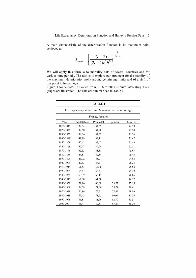
Figure 3 for females in France from 1816 to 2007 is quite interesting. Four

graphs are illustrated. The data are summarized in Table I.

TABLE I

Life expectancy at birth and Maximum deterioration age

France, females

Year HM-database IM-model 3p-model Max Det

1816-1819 39,54 34,69 74,79

1820-1829 39,58 34,98 75,20

1830-1839 39,66 37,39 75,36

1840-1849 41,19 39,15 75,67

1850-1859 40,43 39,67 75,43

1860-1869 42,27 39,74 75,11

1870-1879 42,33 41,51 75,63

1880-1889 44,81 42,54 75,45

1890-1899 46,72 45,77 74,98

1900-1909 49,83 48,87 75,23

1910-1919 51,53 54,06 75,53

1920-1929 56,41 55,41 75,79

1930-1939 60,89 60,13 76,06

1940-1949 62,00 61,50 76,37

1950-1959 71,16 66,68 73,72 77,15

1960-1969 74,59 71,60 75,78 78,61

1970-1979 76,89 75,25 77,54 79,86

1980-1989 79,45 78,75 80,04 81,24

1990-1999 81,81 81,96 82,70 83,51

2000-2007 83,47 82,87 83,27 85,26

C. H. Skiadas 6

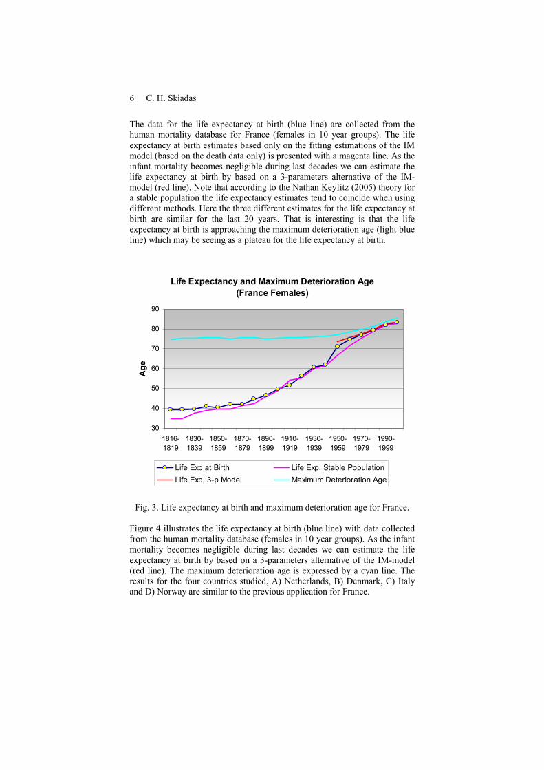
The data for the life expectancy at birth (blue line) are collected from the

human mortality database for France (females in 10 year groups). The life

expectancy at birth estimates based only on the fitting estimations of the IM

model (based on the death data only) is presented with a magenta line. As the

infant mortality becomes negligible during last decades we can estimate the

life expectancy at birth by based on a 3-parameters alternative of the IM-

model (red line). Note that according to the Nathan Keyfitz (2005) theory for

a stable population the life expectancy estimates tend to coincide when using

different methods. Here the three different estimates for the life expectancy at

birth are similar for the last 20 years. That is interesting is that the life

expectancy at birth is approaching the maximum deterioration age (light blue

line) which may be seeing as a plateau for the life expectancy at birth.

Life Expectancy and Maximum Deterioration Age

(France Females)

30

40

50

60

70

80

90

1816-

1819

1830-

1839

1850-

1859

1870-

1879

1890-

1899

1910-

1919

1930-

1939

1950-

1959

1970-

1979

1990-

1999

Age

Life Exp at Birth Life Exp, Stable Population

Life Exp, 3-p Model Maximum Deterioration Age

Fig. 3. Life expectancy at birth and maximum deterioration age for France.

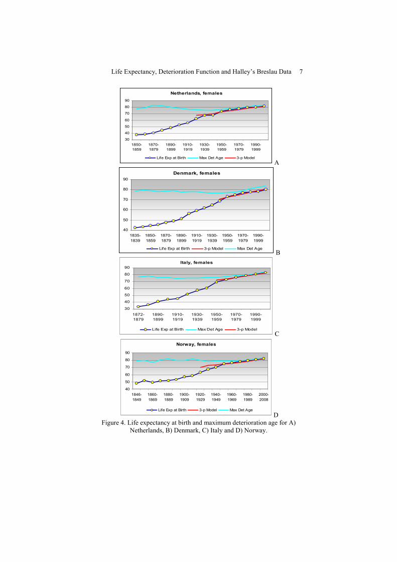
Figure 4 illustrates the life expectancy at birth (blue line) with data collected

from the human mortality database (females in 10 year groups). As the infant

mortality becomes negligible during last decades we can estimate the life

expectancy at birth by based on a 3-parameters alternative of the IM-model

(red line). The maximum deterioration age is expressed by a cyan line. The

results for the four countries studied, A) Netherlands, B) Denmark, C) Italy

and D) Norway are similar to the previous application for France.


Netherlands, females

30

40

50

60

70

80

90

1850-

1859

1870-

1879

1890-

1899

1910-

1919

1930-

1939

1950-

1959

1970-

1979

1990-

1999

Life Exp at Birth Max Det Age 3-p Model

A

Denmark, females

40

50

60

70

80

90

1835-

1839

1850-

1859

1870-

1879

1890-

1899

1910-

1919

1930-

1939

1950-

1959

1970-

1979

1990-

1999

Life Exp at Birth 3-p Model Max Det Age

B

Italy, females

30

40

50

60

70

80

90

1872-

1879

1890-

1899

1910-

1919

1930-

1939

1950-

1959

1970-

1979

1990-

1999

Life Exp at Birth Max Det Age 3-p Model

C

Norway, females

40

50

60

70

80

90

1846-

1849

1860-

1869

1880-

1889

1900-

1909

1920-

1929

1940-

1949

1960-

1969

1980-

1989

2000-

2008

Life Exp at Birth 3-p Model Max Det Age

D

Figure 4. Life expectancy at birth and maximum deterioration age for A)

Netherlands, B) Denmark, C) Italy and D) Norway.

C. H. Skiadas 8

Maximum Deterioration Age (Females)

72,00

74,00

76,00

78,00

80,00

82,00

84,00

86,00

1830-

1839

1850-

1859

1870-

1879

1890-

1899

1910-

1919

1930-

1939

1950-

1959

1970-

1979

1990-

1999

Australia

Belgium

Canada

Denmark

Finland

France

Italy

Japan

Netherlands

Norway

Spain

Sweden

Switzerland

UK

USA

Mean

Fig. 5. Maximum deterioration age for 15 countries and mean value.

The age year where the maximum value for the deterioration function is

achieved for females in various countries and for several time periods is

illustrated in Figure 5. The data for females from various countries for 10

year periods from the human mortality data base are used and the Infant

Mortality First Exit Density Model (IM-model) is applied. The maximum

deterioration age for females was between 72 – 84 years from 1830 to 1950

for the countries studied (Table II). For all the cases a continuous growth

appears for the maximum deterioration age after 1950 until now. That is

more important is that the mean value of the maximum deterioration age was

between 76 and 78 years for 140 years (1830-1970) irrespective of the

fluctuations in the life expectancy supporting the argument for an aging

mechanism in the human genes. However, the scientific and medical

developments after 1950 gave rise in a gradual increase of the level of the

maximum deterioration age from 77 to 84 years in the last 60 years (1950-

2010).

C. H. Skiadas 10

Stability of the Deterioration Function Characteristics

The derivation of the deterioration function of a population allows us to make

early estimates for the life expectancy. The main assumption is based on

accepting a theory for an internal deterioration mechanism driven by a code

which governs the life expectancy. If this assumption holds the deterioration

function should include information for the future life expectancy even when

using data from periods when the mean life duration was relatively small. In

the previous chapter we have found that the maximum value of the

deterioration function in many countries was set at high levels even when

dealing with mortality data coming from various countries and from the last

two centuries.

The next very important point is to estimate the total effect of the

deterioration to a population in the course of the life time termed as DTR.

This is expressed by the following summation formula:

∑∫ ≈=tt

ttKdtttKDTR0

0)()(

Where t is the age and K(t) is the deterioration function.

The last formula expresses the expectation that an individual will survive

from the deterioration caused in his organism by the deterioration

mechanism. The result is given in years of age in a Table like the classical

life tables. The deterioration function is estimated from 0 to 117 years a limit

set according to the existing death data sets. The estimated life expectancy

levels are not the specific levels at the dates of the calculation but refer to

future dates when the external influences, illnesses and societal causes will be

reduced to a minimum following the advancement of our population status.

The life expectancy levels seem to be reached in the recent years in some

countries and in the forthcoming decades for others.

DTR will be a strong indicator for the level of life expectancy of a specific

population mainly caused by the DNA and genes. Due to its characteristics

DTR can also be estimated from only mortality data (number of deaths per

age or death distribution) thus making simpler the handling of this indicator

even when population data are missing or are not well estimated. Another

important point of the last formula is that we can find an estimator of the life

expectancy in various age periods and to construct a life table. As it is

expected the existence of a deterioration law will result in a population

distribution over time thus making possible the construction of life tables by

using the population distribution resulting from the deterioration law.

As the introduction of the deterioration function and the DTR indicator are

quite new terms introduced when using the stochastic modeling techniques

and the first exit time or hitting time theory we have applied the DTR and

other forms resulting from the deterioration function to the mortality data for

countries included in the Human Mortality Database (HMD). A main


advantage by using these data sets is that are systematically collected and

developed as to be able to make applications and comparisons between

countries. The death data for 10-year periods are preferred as to avoid local

fluctuations. However, the results are also strong when using and the other

data sets from HMD for 5-year of 1-year periods.

DTR for 15 Countries (females)

78

79

80

81

82

83

84

85

86

87

1830-

1839

1850-

1859

1870-

1879

1890-

1899

1910-

1919

1930-

1939

1950-

1959

1970-

1979

1990-

1999

France

Finland

Denmark

Belgium

Norway

Italy

Netherlands

Spain

Sweden

Switzerland

UK

USA

Australia

Canada

Japan

Mean

Fig. 6. DTR for 15 countries and mean value.

The DTR is estimated for 15 countries for large time periods. As it is

presented in Figure 6 the DTR for 150 years from 1830 to 1980 was between

78 and 84 years of age with the mean value to be from 79.80 to 81.98 years

(see Table III). The lowest value 79.80 years was achieved the period 1950-

1959. The main conclusion is that the DTR can be used as a measure of the

future life expectancy levels. An example is based on the estimates for

Sweden from 1751. The same method can be applied for other countries.

C. H. Skiadas 12


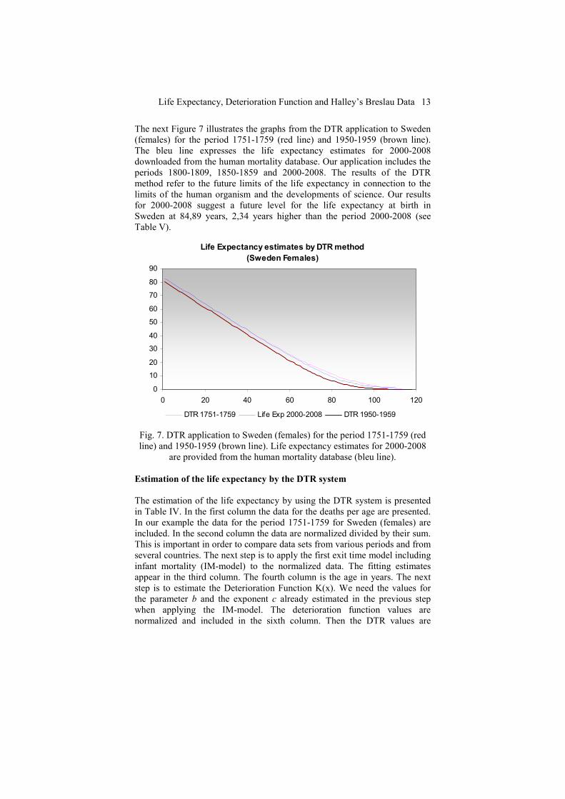
The next Figure 7 illustrates the graphs from the DTR application to Sweden

(females) for the period 1751-1759 (red line) and 1950-1959 (brown line).

The bleu line expresses the life expectancy estimates for 2000-2008

downloaded from the human mortality database. Our application includes the

periods 1800-1809, 1850-1859 and 2000-2008. The results of the DTR

method refer to the future limits of the life expectancy in connection to the

limits of the human organism and the developments of science. Our results

for 2000-2008 suggest a future level for the life expectancy at birth in

Sweden at 84,89 years, 2,34 years higher than the period 2000-2008 (see

Table V).

Life Expectancy estimates by DTR method

(Sweden Females)

0

10

20

30

40

50

60

70

80

90

0 20 40 60 80 100 120

DTR 1751-1759 Life Exp 2000-2008 DTR 1950-1959

Fig. 7. DTR application to Sweden (females) for the period 1751-1759 (red

line) and 1950-1959 (brown line). Life expectancy estimates for 2000-2008

are provided from the human mortality database (bleu line).

Estimation of the life expectancy by the DTR system

The estimation of the life expectancy by using the DTR system is presented

in Table IV. In the first column the data for the deaths per age are presented.

In our example the data for the period 1751-1759 for Sweden (females) are

included. In the second column the data are normalized divided by their sum.

This is important in order to compare data sets from various periods and from

several countries. The next step is to apply the first exit time model including

infant mortality (IM-model) to the normalized data. The fitting estimates

appear in the third column. The fourth column is the age in years. The next

step is to estimate the Deterioration Function K(x). We need the values for

the parameter b and the exponent c already estimated in the previous step

when applying the IM-model. The deterioration function values are

normalized and included in the sixth column. Then the DTR values are

C. H. Skiadas 14

estimated in the seventh column. These values are computed as a

multiplication: xK(x) and then are normalized and stored in the eight column.

Then the DTR survival curve is estimated and included in column nine. We

apply the following formula for the survival curve (SC):

∑−

−=1

0

)(1x

x xxKSC .

The final step is the formulation of the tenth column including the DTR life

expectancy list according to age from the survival curve. The life expectancy

ex at age x is calculated by: ∑ ∑−=n x

xxx SCSCe0 0

, where n was selected

the age 117 as a level according to our experience. However, the selection of

a different age level will change the estimates for the life expectancy. The

best approach will be the selection of a level age which is in accordance to

reality.

The results of the application of the DTR method for various time periods in Sweden

for females are summarized in Table V. The estimated life expectancy values are very

close to that achieved in recent years as is also illustrated in Figure 8 thus supporting

our argument for using the DTR method to forecasts the future trends of life

expectancy. Even from the period 1751-1759 we can estimate a life expectancy at

birth at the level of 82.92 years for Sweden, females. This value is very close to that

of the period 2000-2008 (82.55 years).


1 7 5 1 -

1 7 5 9

D a ta

D a ta

N o rm a lis

e d

IM M o d e l

E s t im a te s

Y e a r

xK (x )

K (x )

N o rm a lis e dxK (x)

xK (x)

N o rm a lis e d

S u rv iv a l

c u rv e

L ife

E xp e c t

a n c y

5 7 4 2 5 0 ,2 47 3 0 ,2 3 1 7 0 4 ,5 6E -0 5 6 ,0 0 4E -0 5 0 0 1 8 2 ,9 2

1 4 4 3 8 0 ,0 62 2 0 ,0 8 7 3 1 0 ,0 0 0 1 1 2 0 ,0 0 0 14 7 8 0 ,0 0 0 1 4 8 2 ,0 4 4E -0 6 1 8 1 ,9 2

9 4 6 7 0 ,0 40 8 0 ,0 4 8 6 2 0 ,0 0 0 1 9 0 ,0 0 0 25 0 5 0 ,0 0 0 5 0 1 6 ,9 2 6E -0 6 1 8 0 ,9 2

6 7 3 9 0 ,0 29 0 0 ,0 3 1 9 3 0 ,0 0 0 2 7 6 0 ,0 0 0 3 6 4 0 ,0 0 1 0 9 2 1 ,5 1E -0 5 0 ,99 9 9 9 7 9 ,9 2

4 9 1 8 0 ,0 21 2 0 ,0 2 3 1 4 0 ,0 0 0 3 6 9 0 ,0 0 0 48 6 6 0 ,0 0 1 9 4 6 2 ,6 9 1E -0 5 0 ,99 9 9 8 7 8 ,9 2

3 6 1 9 0 ,0 15 6 0 ,0 1 7 7 5 0 ,0 0 0 4 6 8 0 ,0 0 0 61 6 7 0 ,0 0 3 0 8 3 4 ,2 6 4E -0 5 0 ,99 9 9 5 7 7 ,9 2

2 6 2 3 0 ,0 11 3 0 ,0 1 4 2 6 0 ,0 0 0 5 7 2 0 ,0 0 0 75 3 5 0 ,0 0 4 5 2 1 6 ,2 5 2E -0 5 0 ,99 9 9 1 7 6 ,9 2

1 8 7 5 0 ,0 08 1 0 ,0 1 1 7 7 0 ,0 0 0 6 8 0 ,0 0 0 89 6 4 0 ,0 0 6 2 7 5 8 ,6 7 6E -0 5 0 ,99 9 8 4 7 5 ,9 2

1 3 7 5 0 ,0 05 9 0 ,0 1 0 0 8 0 ,0 0 0 7 9 3 0 ,0 0 1 04 4 7 0 ,0 0 8 3 5 7 0 ,0 0 0 11 5 6 0 ,99 9 7 6 7 4 ,9 2

1 1 2 4 0 ,0 04 8 0 ,0 0 8 7 9 0 ,0 0 0 9 0 9 0 ,0 0 1 1 9 8 0 ,0 1 0 7 8 2 0 ,0 0 0 14 9 1 0 ,99 9 6 4 7 3 ,9 2

1 0 7 8 0 ,0 04 6 0 ,0 0 7 7 1 0 0 ,0 0 1 0 2 9 0 ,0 0 1 3 5 6 0 ,0 13 5 6 0 ,0 0 0 18 7 5 0 ,99 9 4 9 7 2 ,9 2

1 0 6 5 0 ,0 04 6 0 ,0 0 6 9 1 1 0 ,0 0 1 1 5 2 0 ,0 0 1 51 8 4 0 ,0 1 6 7 0 2 0 ,0 0 0 2 3 1 0 ,9 9 9 3 7 1 ,9 2

1 0 4 4 0 ,0 04 5 0 ,0 0 6 3 1 2 0 ,0 0 1 2 7 9 0 ,0 0 1 68 4 9 0 ,0 2 0 2 1 8 0 ,0 0 0 27 9 6 0 ,9 9 9 0 7 7 0 ,9 2

1 0 1 3 0 ,0 04 4 0 ,0 0 5 8 1 3 0 ,0 0 1 4 0 8 0 ,0 0 1 85 5 2 0 ,0 2 4 1 1 7 0 ,0 0 0 33 3 5 0 ,9 9 8 7 9 6 9 ,9 2

9 7 3 0 ,0 04 2 0 ,0 0 5 4 1 4 0 ,0 0 1 5 4 0 ,0 0 2 02 9 2 0 ,0 2 8 4 0 9 0 ,0 0 0 39 2 8 0 ,99 8 4 6 6 8 ,9 2

9 2 9 0 ,0 04 0 0 ,0 0 5 1 1 5 0 ,0 0 1 6 7 5 0 ,0 0 2 20 6 7 0 ,0 3 3 1 0 ,0 0 0 45 7 7 0 ,99 8 0 7 6 7 ,9 3

8 9 9 0 ,0 03 9 0 ,0 0 4 9 1 6 0 ,0 0 1 8 1 2 0 ,0 0 2 38 7 5 0 ,0 3 8 1 9 9 0 ,0 0 0 52 8 2 0 ,9 9 7 6 1 6 6 ,9 3

8 8 8 0 ,0 03 8 0 ,0 0 4 7 1 7 0 ,0 0 1 9 5 2 0 ,0 0 2 57 1 4 0 ,0 4 3 7 1 4 0 ,0 0 0 60 4 5 0 ,9 9 7 0 8 6 5 ,9 3

8 9 7 0 ,0 03 9 0 ,0 0 4 6 1 8 0 ,0 0 2 0 9 3 0 ,0 0 2 75 8 4 0 ,0 4 9 6 5 1 0 ,0 0 0 68 6 5 0 ,9 9 6 4 8 6 4 ,9 3

9 2 6 0 ,0 04 0 0 ,0 0 4 5 1 9 0 ,0 0 2 2 3 7 0 ,0 0 2 94 8 2 0 ,0 5 6 0 1 6 0 ,0 0 0 77 4 6 0 ,9 9 5 7 9 6 3 ,9 4

9 6 9 0 ,0 04 2 0 ,0 0 4 4 2 0 0 ,0 0 2 3 8 4 0 ,0 0 3 14 0 8 0 ,0 6 2 8 1 7 0 ,0 0 0 86 8 6 0 ,9 9 5 0 2 6 2 ,9 4

1 0 1 1 0 ,0 04 4 0 ,0 0 4 4 2 1 0 ,0 0 2 5 3 2 0 ,0 0 3 33 6 1 0 ,0 7 0 0 5 8 0 ,0 0 0 96 8 7 0 ,9 9 4 1 5 6 1 ,9 5

1 0 4 6 0 ,0 04 5 0 ,0 0 4 4 2 2 0 ,0 0 2 6 8 2 0 ,0 0 3 53 3 8 0 ,0 7 7 7 4 4 0 ,0 0 1 0 7 5 0 ,99 3 1 8 6 0 ,9 5

1 0 7 6 0 ,0 04 6 0 ,0 0 4 4 2 3 0 ,0 0 2 8 3 4 0 ,0 0 3 7 3 4 0 ,0 8 5 8 8 2 0 ,0 0 1 18 7 5 0 ,9 9 2 1 5 9 ,9 6

1 1 0 0 0 ,0 04 7 0 ,0 0 4 5 2 4 0 ,0 0 2 9 8 7 0 ,0 0 3 93 6 4 0 ,0 9 4 4 7 4 0 ,0 0 1 30 6 3 0 ,9 9 0 9 2 5 8 ,9 7

1 1 2 2 0 ,0 04 8 0 ,0 0 4 5 2 5 0 ,0 0 3 1 4 3 0 ,0 0 4 14 1 1 0 ,1 0 3 5 2 6 0 ,0 0 1 43 1 5 0 ,9 8 9 6 1 5 7 ,9 7

1 1 5 8 0 ,0 05 0 0 ,0 0 4 6 2 6 0 ,0 0 3 3 0 ,0 0 4 34 7 7 0 ,1 1 3 0 4 1 0 ,0 0 1 56 3 1 0 ,98 8 1 8 5 6 ,9 9

1 2 1 4 0 ,0 05 2 0 ,0 0 4 7 2 7 0 ,0 0 3 4 5 8 0 ,0 0 4 55 6 3 0 ,1 2 3 0 2 1 0 ,0 0 1 70 1 1 0 ,9 8 6 6 2 5 6 ,0 0

1 2 8 8 0 ,0 05 5 0 ,0 0 4 8 2 8 0 ,0 0 3 6 1 8 0 ,0 0 4 76 6 8 0 ,1 33 4 7 0 ,0 0 1 84 5 6 0 ,98 4 9 1 5 5 ,0 1

1 3 8 2 0 ,0 06 0 0 ,0 0 4 9 2 9 0 ,0 0 3 7 7 9 0 ,0 0 4 97 8 9 0 ,1 4 4 3 8 9 0 ,0 0 1 99 6 5 0 ,9 8 3 0 7 5 4 ,0 3

1 4 8 2 0 ,0 06 4 0 ,0 0 5 0 3 0 0 ,0 0 3 9 4 1 0 ,0 0 5 19 2 7 0 ,1 55 7 8 0 ,0 0 2 1 5 4 0 ,98 1 0 7 5 3 ,0 4

1 5 3 7 0 ,0 06 6 0 ,0 0 5 1 3 1 0 ,0 0 4 1 0 4 0 ,0 0 5 40 7 8 0 ,1 6 7 6 4 3 0 ,0 0 2 31 8 1 0 ,9 7 8 9 2 5 2 ,0 6

1 5 3 5 0 ,0 06 6 0 ,0 0 5 3 3 2 0 ,0 0 4 2 6 8 0 ,0 0 5 62 4 3 0 ,1 7 9 9 7 9 0 ,0 0 2 48 8 7 0 ,9 7 6 6 5 1 ,0 8

1 4 7 6 0 ,0 06 4 0 ,0 0 5 4 3 3 0 ,0 0 4 4 3 4 0 ,0 0 5 8 4 2 0 ,1 9 2 7 8 7 0 ,0 0 2 66 5 8 0 ,97 4 1 1 5 0 ,1 1

1 3 5 9 0 ,0 05 9 0 ,0 0 5 6 3 4 0 ,0 0 4 6 0 ,0 0 6 06 0 8 0 ,2 0 6 0 6 6 0 ,0 0 2 84 9 4 0 ,97 1 4 5 4 9 ,1 3

1 2 0 7 0 ,0 05 2 0 ,0 0 5 8 3 5 0 ,0 0 4 7 6 6 0 ,0 0 6 28 0 4 0 ,2 1 9 8 1 3 0 ,0 0 3 03 9 5 0 ,9 6 8 6 4 8 ,1 6

1 1 0 3 0 ,0 04 7 0 ,0 0 5 9 3 6 0 ,0 0 4 9 3 4 0 ,0 0 6 50 0 7 0 ,2 3 4 0 2 7 0 ,0 0 3 2 3 6 0 ,96 5 5 6 4 7 ,1 9

1 0 6 8 0 ,0 04 6 0 ,0 0 6 1 3 7 0 ,0 0 5 1 0 1 0 ,0 0 6 72 1 7 0 ,2 4 8 7 0 2 0 ,0 0 3 43 8 9 0 ,9 6 2 3 2 4 6 ,2 3

1 1 0 4 0 ,0 04 8 0 ,0 0 6 3 3 8 0 ,0 0 5 2 6 9 0 ,0 0 6 9 4 3 0 ,2 6 3 8 3 4 0 ,0 0 3 64 8 2 0 ,95 8 8 8 4 5 ,2 6

1 2 0 9 0 ,0 05 2 0 ,0 0 6 5 3 9 0 ,0 0 5 4 3 7 0 ,0 0 7 16 4 5 0 ,2 7 9 4 1 7 0 ,0 0 3 86 3 6 0 ,9 5 5 2 3 4 4 ,3 1

1 3 6 2 0 ,0 05 9 0 ,0 0 6 7 4 0 0 ,0 0 5 6 0 5 0 ,0 0 7 38 6 1 0 ,2 9 5 4 4 4 0 ,0 0 4 08 5 3 0 ,9 5 1 3 7 4 3 ,3 5

1 4 6 9 0 ,0 06 3 0 ,0 0 6 9 4 1 0 ,0 0 5 7 7 4 0 ,0 0 7 60 7 5 0 ,3 1 1 9 0 8 0 ,0 0 4 31 2 9 0 ,9 4 7 2 9 4 2 ,4 0

1 5 0 9 0 ,0 06 5 0 ,0 0 7 1 4 2 0 ,0 0 5 9 4 1 0 ,0 0 7 82 8 6 0 ,3 2 8 7 9 9 0 ,0 0 4 54 6 5 0 ,9 4 2 9 7 4 1 ,4 5

1 4 8 1 0 ,0 06 4 0 ,0 0 7 3 4 3 0 ,0 0 6 1 0 9 0 ,0 0 8 0 4 9 0 ,3 4 6 1 0 7 0 ,0 0 4 78 5 8 0 ,93 8 4 3 4 0 ,5 1

1 3 8 6 0 ,0 06 0 0 ,0 0 7 6 4 4 0 ,0 0 6 2 7 5 0 ,0 0 8 26 8 6 0 ,3 63 8 2 0 ,0 0 5 03 0 7 0 ,93 3 6 4 3 9 ,5 7

1 2 4 5 0 ,0 05 4 0 ,0 0 7 8 4 5 0 ,0 0 6 4 4 1 0 ,0 0 8 48 7 2 0 ,3 8 1 9 2 5 0 ,0 0 5 28 1 1 0 ,9 2 8 6 1 3 8 ,6 4

1 1 4 4 0 ,0 04 9 0 ,0 0 8 0 4 6 0 ,0 0 6 6 0 6 0 ,0 0 8 70 4 5 0 ,4 0 0 4 0 8 0 ,0 0 5 53 6 7 0 ,9 2 3 3 3 3 7 ,7 1

1 1 0 6 0 ,0 04 8 0 ,0 0 8 2 4 7 0 ,0 0 6 7 7 0 ,0 0 8 92 0 3 0 ,4 1 9 2 5 3 0 ,0 0 5 79 7 2 0 ,91 7 7 9 3 6 ,7 8

1 1 2 9 0 ,0 04 9 0 ,0 0 8 4 4 8 0 ,0 0 6 9 3 2 0 ,0 0 9 13 4 2 0 ,4 3 8 4 4 3 0 ,0 0 6 06 2 6 0 ,9 1 1 9 9 3 5 ,8 7

1 2 1 5 0 ,0 05 2 0 ,0 0 8 7 4 9 0 ,0 0 7 0 9 3 0 ,0 0 9 34 6 1 0 ,4 5 7 9 5 9 0 ,0 0 6 33 2 4 0 ,9 0 5 9 3 3 4 ,9 5

1 3 4 6 0 ,0 05 8 0 ,0 0 8 9 5 0 0 ,0 0 7 2 5 2 0 ,0 0 9 55 5 6 0 ,4 77 7 8 0 ,0 0 6 60 6 5 0 ,8 9 9 6 3 4 ,0 5

1 4 5 0 0 ,0 06 2 0 ,0 0 9 1 5 1 0 ,0 0 7 4 0 9 0 ,0 0 9 76 2 5 0 ,4 9 7 8 8 6 0 ,0 0 6 88 4 5 0 ,8 9 2 9 9 3 3 ,1 5

1 5 0 9 0 ,0 06 5 0 ,0 0 9 3 5 2 0 ,0 0 7 5 6 4 0 ,0 0 9 96 6 4 0 ,5 1 8 2 5 3 0 ,0 0 7 16 6 2 0 ,8 8 6 1 1 3 2 ,2 6

1 5 2 4 0 ,0 06 6 0 ,0 0 9 5 5 3 0 ,0 0 7 7 1 6 0 ,0 1 0 16 7 1 0 ,5 3 8 8 5 5 0 ,0 0 7 4 5 1 0 ,87 8 9 4 3 1 ,3 7

1 4 9 4 0 ,0 06 4 0 ,0 0 9 7 5 4 0 ,0 0 7 8 6 6 0 ,0 1 0 36 4 2 0 ,5 5 9 6 6 7 0 ,0 0 7 73 8 8 0 ,8 7 1 4 9 3 0 ,4 9

1 4 3 8 0 ,0 06 2 0 ,0 0 9 9 5 5 0 ,0 0 8 0 1 2 0 ,0 1 0 55 7 5 0 ,5 80 6 6 0 ,0 0 8 02 9 1 0 ,86 3 7 5 2 9 ,6 2

1 4 3 1 0 ,0 06 2 0 ,0 1 0 1 5 6 0 ,0 0 8 1 5 6 0 ,0 1 0 74 6 5 0 ,6 0 1 8 0 5 0 ,0 0 8 32 1 5 0 ,8 5 5 7 2 2 8 ,7 6

1 4 9 1 0 ,0 06 4 0 ,0 1 0 2 5 7 0 ,0 0 8 2 9 6 0 ,0 1 0 9 3 1 0 ,6 23 0 7 0 ,0 0 8 61 5 5 0 ,8 4 7 4 2 7 ,9 0

1 6 1 9 0 ,0 07 0 0 ,0 1 0 4 5 8 0 ,0 0 8 4 3 2 0 ,0 1 1 11 0 7 0 ,6 4 4 4 2 3 0 ,0 0 8 91 0 8 0 ,8 3 8 7 9 2 7 ,0 5

1 8 1 4 0 ,0 07 8 0 ,0 1 0 6 5 9 0 ,0 0 8 5 6 5 0 ,0 1 1 28 5 2 0 ,6 65 8 3 0 ,0 0 9 20 6 8 0 ,82 9 8 8 2 6 ,2 1

2 0 5 3 0 ,0 08 8 0 ,0 1 0 7 6 0 0 ,0 0 8 6 9 3 0 ,0 1 1 45 4 3 0 ,6 8 7 2 5 5 0 ,0 0 9 5 0 3 0 ,82 0 6 7 2 5 ,3 8

TAB LE IV

D TR S ys tem (S w e d e n , F em a le s )

C. H. Skiadas 16

2246 0,0097 0,0108 61 0,008817 0,0116174 0,708662 0,0097991 0,81117 24,56

2371 0,0102 0,0109 62 0,008936 0,0117744 0,730013 0,0100943 0,80137 23,75

2428 0,0105 0,0110 63 0,00905 0,0119249 0,751269 0,0103882 0,79127 22,95

2416 0,0104 0,0111 64 0,009159 0,0120686 0,77239 0,0106803 0,78088 22,16

2357 0,0102 0,0111 65 0,009263 0,0122052 0,793336 0,0109699 0,7702 21,38

2343 0,0101 0,0112 66 0,009361 0,0123343 0,814064 0,0112565 0,75923 20,61

2395 0,0103 0,0112 67 0,009453 0,0124557 0,834534 0,0115395 0,74798 19,85

2512 0,0108 0,0111 68 0,009539 0,0125692 0,854702 0,0118184 0,73644 19,10

2696 0,0116 0,0111 69 0,009619 0,0126743 0,874527 0,0120926 0,72462 18,36

2918 0,0126 0,0110 70 0,009692 0,0127709 0,893965 0,0123613 0,71253 17,64

3060 0,0132 0,0109 71 0,009759 0,0128588 0,912975 0,0126242 0,70017 16,93

3096 0,0133 0,0108 72 0,009819 0,0129377 0,931515 0,0128806 0,68754 16,23

3025 0,0130 0,0107 73 0,009872 0,0130074 0,949543 0,0131298 0,67466 15,54

2846 0,0123 0,0105 74 0,009917 0,0130678 0,967019 0,0133715 0,66153 14,87

2588 0,0111 0,0103 75 0,009956 0,0131187 0,983905 0,013605 0,64816 14,20

2358 0,0102 0,0101 76 0,009987 0,01316 1,000161 0,0138298 0,63455 13,56

2184 0,0094 0,0098 77 0,010011 0,0131916 1,015751 0,0140453 0,62072 12,92

2065 0,0089 0,0096 78 0,010028 0,0132133 1,030641 0,0142512 0,60668 12,30

2003 0,0086 0,0093 79 0,010037 0,0132253 1,044797 0,014447 0,59243 11,69

1979 0,0085 0,0089 80 0,010039 0,0132273 1,058188 0,0146321 0,57798 11,10

1927 0,0083 0,0086 81 0,010033 0,0132196 1,070785 0,0148063 0,56335 10,52

1828 0,0079 0,0082 82 0,010019 0,013202 1,082563 0,0149692 0,54854 9,96

1683 0,0072 0,0079 83 0,009999 0,0131747 1,093498 0,0151204 0,53357 9,41

1492 0,0064 0,0075 84 0,009971 0,0131377 1,103567 0,0152596 0,51845 8,88

1267 0,0055 0,0071 85 0,009935 0,0130912 1,112754 0,0153866 0,50319 8,36

1061 0,0046 0,0067 86 0,009893 0,0130354 1,121042 0,0155013 0,48781 7,86

887 0,0038 0,0062 87 0,009844 0,0129703 1,12842 0,0156033 0,47231 7,37

743 0,0032 0,0058 88 0,009787 0,0128963 1,134876 0,0156925 0,4567 6,90

631 0,0027 0,0054 89 0,009725 0,0128136 1,140407 0,015769 0,44101 6,44

586 0,0025 0,0050 90 0,009655 0,0127223 1,145007 0,0158326 0,42524 6,00

484 0,0021 0,0046 91 0,00958 0,0126228 1,148676 0,0158834 0,40941 5,57

395 0,0017 0,0042 92 0,009498 0,0125154 1,151418 0,0159213 0,39352 5,16

318 0,0014 0,0038 93 0,009411 0,0124004 1,153238 0,0159464 0,3776 4,77

252 0,0011 0,0034 94 0,009318 0,0122781 1,154144 0,015959 0,36166 4,39

197 0,0008 0,0031 95 0,00922 0,0121489 1,154147 0,015959 0,3457 4,03

151 0,0007 0,0028 96 0,009117 0,0120131 1,153262 0,0159468 0,32974 3,68

115 0,0005 0,0024 97 0,009009 0,0118712 1,151505 0,0159225 0,31379 3,36

86 0,0004 0,0021 98 0,008897 0,0117234 1,148894 0,0158864 0,29787 3,04

63 0,0003 0,0019 99 0,008781 0,0115702 1,145451 0,0158388 0,28198 2,74

45 0,0002 0,0016 100 0,008661 0,011412 1,141199 0,01578 0,26614 2,46

32 0,0001 0,0014 101 0,008537 0,0112491 1,136163 0,0157103 0,25036 2,20

23 0,0001 0,0012 102 0,00841 0,0110821 1,13037 0,0156302 0,23465 1,95

15 0,0001 0,0010 103 0,008281 0,0109111 1,123847 0,01554 0,21902 1,71

10 0,0000 0,0008 104 0,008148 0,0107368 1,116625 0,0154402 0,20348 1,49

6 0,0000 0,0007 105 0,008014 0,0105594 1,108734 0,0153311 0,18804 1,29

3 0,0000 0,0006 106 0,007877 0,0103793 1,100205 0,0152131 0,17271 1,10

1 0,0000 0,0005 107 0,007739 0,0101969 1,091072 0,0150868 0,1575 0,93

0 0,0000 0,0004 108 0,007599 0,0100127 1,081367 0,0149526 0,14241 0,77

0 0,0000 0,0003 109 0,007458 0,0098268 1,071124 0,014811 0,12746 0,63

0 0,0000 0,0002 110 0,007316 0,0096398 1,060376 0,0146624 0,11265 0,50

0,0000 0,0002 111 0,007173 0,0094519 1,049157 0,0145073 0,09799 0,39

0,0000 0,0001 112 0,00703 0,0092634 1,037502 0,0143461 0,08348 0,29

0,0000 0,0001 113 0,006887 0,0090747 1,025442 0,0141793 0,06913 0,21

0,0000 0,0001 114 0,006744 0,0088861 1,013012 0,0140075 0,05495 0,14

0,0000 0,0001 115 0,006601 0,0086978 1,000245 0,0138309 0,04095 0,08

0,0000 0,0000 116 0,006459 0,0085101 0,987171 0,0136501 0,02712 0,04

0,0000 0,0000 117 0,006317 0,0083233 0,973824 0,0134656 0,01347 0,01


Y e a r

x

1 7 5 1 -

1 7 5 9

1 8 0 0 -

1 8 0 9

1 8 5 0 -

1 8 5 9

1 9 0 0 -

1 9 0 91 9 5 0 -1 9 5 9

2 0 0 0 -

2 0 0 8

L i fe E x p

2 0 0 0 -2 0 0 8

0 8 2 ,9 2 8 1 ,2 1 8 0 ,7 6 8 0 ,4 2 8 0 ,0 6 8 4 ,8 9 8 2 ,5 5

1 8 1 ,9 2 8 0 ,2 1 7 9 ,7 6 7 9 ,4 2 7 9 ,0 6 8 3 ,8 9 8 1 ,7 7

2 8 0 ,9 2 7 9 ,2 1 7 8 ,7 6 7 8 ,4 2 7 8 ,0 6 8 2 ,8 9 8 0 ,7 9

3 7 9 ,9 2 7 8 ,2 1 7 7 ,7 6 7 7 ,4 2 7 7 ,0 6 8 1 ,8 9 7 9 ,8

4 7 8 ,9 2 7 7 ,2 1 7 6 ,7 6 7 6 ,4 2 7 6 ,0 6 8 0 ,8 9 7 8 ,8 1

5 7 7 ,9 2 7 6 ,2 1 7 5 ,7 6 7 5 ,4 2 7 5 ,0 6 7 9 ,8 9 7 7 ,8 2

6 7 6 ,9 2 7 5 ,2 1 7 4 ,7 6 7 4 ,4 2 7 4 ,0 6 7 8 ,8 9 7 6 ,8 3

7 7 5 ,9 2 7 4 ,2 1 7 3 ,7 6 7 3 ,4 2 7 3 ,0 6 7 7 ,8 9 7 5 ,8 4

8 7 4 ,9 2 7 3 ,2 1 7 2 ,7 6 7 2 ,4 2 7 2 ,0 6 7 6 ,8 9 7 4 ,8 4

9 7 3 ,9 2 7 2 ,2 1 7 1 ,7 6 7 1 ,4 2 7 1 ,0 6 7 5 ,8 9 7 3 ,8 5

1 0 7 2 ,9 2 7 1 ,2 1 7 0 ,7 6 7 0 ,4 2 7 0 ,0 6 7 4 ,8 9 7 2 ,8 5

1 1 7 1 ,9 2 7 0 ,2 1 6 9 ,7 6 6 9 ,4 2 6 9 ,0 6 7 3 ,8 9 7 1 ,8 6

1 2 7 0 ,9 2 6 9 ,2 1 6 8 ,7 6 6 8 ,4 2 6 8 ,0 6 7 2 ,8 9 7 0 ,8 6

1 3 6 9 ,9 2 6 8 ,2 1 6 7 ,7 6 6 7 ,4 2 6 7 ,0 6 7 1 ,8 9 6 9 ,8 7

1 4 6 8 ,9 2 6 7 ,2 2 6 6 ,7 6 6 6 ,4 2 6 6 ,0 6 7 0 ,8 9 6 8 ,8 8

1 5 6 7 ,9 3 6 6 ,2 2 6 5 ,7 6 6 5 ,4 2 6 5 ,0 6 6 9 ,8 9 6 7 ,8 8

1 6 6 6 ,9 3 6 5 ,2 2 6 4 ,7 6 6 4 ,4 2 6 4 ,0 6 6 8 ,8 9 6 6 ,9

1 7 6 5 ,9 3 6 4 ,2 2 6 3 ,7 7 6 3 ,4 2 6 3 ,0 6 6 7 ,8 9 6 5 ,9 1

1 8 6 4 ,9 3 6 3 ,2 2 6 2 ,7 7 6 2 ,4 2 6 2 ,0 6 6 6 ,8 9 6 4 ,9 2

1 9 6 3 ,9 4 6 2 ,2 2 6 1 ,7 7 6 1 ,4 2 6 1 ,0 6 6 5 ,8 9 6 3 ,9 4

2 0 6 2 ,9 4 6 1 ,2 3 6 0 ,7 7 6 0 ,4 2 6 0 ,0 6 6 4 ,8 9 6 2 ,9 6

2 1 6 1 ,9 5 6 0 ,2 3 5 9 ,7 7 5 9 ,4 2 5 9 ,0 6 6 3 ,8 9 6 1 ,9 7

2 2 6 0 ,9 5 5 9 ,2 4 5 8 ,7 8 5 8 ,4 2 5 8 ,0 7 6 2 ,8 9 6 0 ,9 9

2 3 5 9 ,9 6 5 8 ,2 4 5 7 ,7 8 5 7 ,4 2 5 7 ,0 7 6 1 ,8 9 6 0

2 4 5 8 ,9 7 5 7 ,2 5 5 6 ,7 9 5 6 ,4 2 5 6 ,0 7 6 0 ,8 9 5 9 ,0 2

2 5 5 7 ,9 7 5 6 ,2 5 5 5 ,7 9 5 5 ,4 2 5 5 ,0 7 5 9 ,8 9 5 8 ,0 3

2 6 5 6 ,9 9 5 5 ,2 6 5 4 ,8 0 5 4 ,4 2 5 4 ,0 7 5 8 ,8 9 5 7 ,0 5

2 7 5 6 ,0 0 5 4 ,2 7 5 3 ,8 1 5 3 ,4 3 5 3 ,0 7 5 7 ,8 9 5 6 ,0 6

2 8 5 5 ,0 1 5 3 ,2 8 5 2 ,8 2 5 2 ,4 3 5 2 ,0 7 5 6 ,8 9 5 5 ,0 8

2 9 5 4 ,0 3 5 2 ,3 0 5 1 ,8 3 5 1 ,4 3 5 1 ,0 7 5 5 ,8 9 5 4 ,0 9

3 0 5 3 ,0 4 5 1 ,3 1 5 0 ,8 4 5 0 ,4 3 5 0 ,0 7 5 4 ,8 9 5 3 ,1 1

3 1 5 2 ,0 6 5 0 ,3 3 4 9 ,8 6 4 9 ,4 3 4 9 ,0 7 5 3 ,8 9 5 2 ,1 2

3 2 5 1 ,0 8 4 9 ,3 5 4 8 ,8 7 4 8 ,4 4 4 8 ,0 7 5 2 ,8 9 5 1 ,1 4

3 3 5 0 ,1 1 4 8 ,3 7 4 7 ,8 9 4 7 ,4 4 4 7 ,0 7 5 1 ,8 9 5 0 ,1 6

3 4 4 9 ,1 3 4 7 ,3 9 4 6 ,9 1 4 6 ,4 4 4 6 ,0 7 5 0 ,8 9 4 9 ,1 7

3 5 4 8 ,1 6 4 6 ,4 1 4 5 ,9 3 4 5 ,4 5 4 5 ,0 8 4 9 ,8 9 4 8 ,1 9

3 6 4 7 ,1 9 4 5 ,4 4 4 4 ,9 6 4 4 ,4 6 4 4 ,0 8 4 8 ,8 9 4 7 ,2 1

3 7 4 6 ,2 3 4 4 ,4 7 4 3 ,9 8 4 3 ,4 6 4 3 ,0 8 4 7 ,8 9 4 6 ,2 4

3 8 4 5 ,2 6 4 3 ,5 1 4 3 ,0 2 4 2 ,4 7 4 2 ,0 9 4 6 ,8 9 4 5 ,2 6

3 9 4 4 ,3 1 4 2 ,5 5 4 2 ,0 5 4 1 ,4 8 4 1 ,0 9 4 5 ,8 9 4 4 ,2 9

4 0 4 3 ,3 5 4 1 ,5 9 4 1 ,0 9 4 0 ,4 9 4 0 ,1 0 4 4 ,8 9 4 3 ,3 1

4 1 4 2 ,4 0 4 0 ,6 3 4 0 ,1 3 3 9 ,5 1 3 9 ,1 1 4 3 ,8 9 4 2 ,3 4

4 2 4 1 ,4 5 3 9 ,6 8 3 9 ,1 7 3 8 ,5 2 3 8 ,1 1 4 2 ,8 9 4 1 ,3 7

4 3 4 0 ,5 1 3 8 ,7 4 3 8 ,2 2 3 7 ,5 4 3 7 ,1 2 4 1 ,8 9 4 0 ,4 1

4 4 3 9 ,5 7 3 7 ,7 9 3 7 ,2 8 3 6 ,5 6 3 6 ,1 3 4 0 ,8 9 3 9 ,4 5

4 5 3 8 ,6 4 3 6 ,8 6 3 6 ,3 4 3 5 ,5 8 3 5 ,1 5 3 9 ,8 9 3 8 ,4 9

4 6 3 7 ,7 1 3 5 ,9 3 3 5 ,4 0 3 4 ,6 0 3 4 ,1 6 3 8 ,8 9 3 7 ,5 3

4 7 3 6 ,7 8 3 5 ,0 0 3 4 ,4 7 3 3 ,6 3 3 3 ,1 8 3 7 ,9 0 3 6 ,5 8

4 8 3 5 ,8 7 3 4 ,0 8 3 3 ,5 5 3 2 ,6 6 3 2 ,2 0 3 6 ,9 0 3 5 ,6 4

4 9 3 4 ,9 5 3 3 ,1 7 3 2 ,6 3 3 1 ,7 0 3 1 ,2 2 3 5 ,9 0 3 4 ,7

5 0 3 4 ,0 5 3 2 ,2 6 3 1 ,7 2 3 0 ,7 4 3 0 ,2 5 3 4 ,9 1 3 3 ,7 6

5 1 3 3 ,1 5 3 1 ,3 6 3 0 ,8 1 2 9 ,7 8 2 9 ,2 8 3 3 ,9 1 3 2 ,8 3

5 2 3 2 ,2 6 3 0 ,4 7 2 9 ,9 1 2 8 ,8 3 2 8 ,3 1 3 2 ,9 2 3 1 ,9 1

5 3 3 1 ,3 7 2 9 ,5 8 2 9 ,0 2 2 7 ,8 9 2 7 ,3 5 3 1 ,9 2 3 0 ,9 8

5 4 3 0 ,4 9 2 8 ,7 1 2 8 ,1 4 2 6 ,9 5 2 6 ,3 9 3 0 ,9 3 3 0 ,0 7

5 5 2 9 ,6 2 2 7 ,8 4 2 7 ,2 7 2 6 ,0 2 2 5 ,4 4 2 9 ,9 4 2 9 ,1 5

5 6 2 8 ,7 6 2 6 ,9 8 2 6 ,4 0 2 5 ,1 0 2 4 ,5 0 2 8 ,9 5 2 8 ,2 4

5 7 2 7 ,9 0 2 6 ,1 2 2 5 ,5 5 2 4 ,1 8 2 3 ,5 6 2 7 ,9 7 2 7 ,3 5

5 8 2 7 ,0 5 2 5 ,2 8 2 4 ,7 0 2 3 ,2 7 2 2 ,6 3 2 6 ,9 8 2 6 ,4 6

5 9 2 6 ,2 1 2 4 ,4 5 2 3 ,8 6 2 2 ,3 7 2 1 ,7 1 2 6 ,0 0 2 5 ,5 7

6 0 2 5 ,3 8 2 3 ,6 2 2 3 ,0 4 2 1 ,4 8 2 0 ,7 9 2 5 ,0 2 2 4 ,7

R e s u l t s f r o m t h e D T R S y s t em f o r t h e F u tu r e L i f e E x p e c ta n c y i n S w e d e n ( F em a le s )

T A B L E V

C. H. Skiadas 18

61 24 ,56 22 ,81 22 ,22 20 ,61 19 ,89 24 ,05 23 ,82

62 23 ,75 22 ,01 21 ,42 19 ,74 19 ,00 23 ,07 22 ,96

63 22 ,95 21 ,22 20 ,63 18 ,88 18 ,11 22 ,11 22 ,1

64 22 ,16 20 ,44 19 ,85 18 ,04 17 ,25 21 ,15 21 ,24

65 21 ,38 19 ,67 19 ,08 17 ,21 16 ,39 20 ,19 20 ,4

66 20 ,61 18 ,91 18 ,32 16 ,40 15 ,55 19 ,24 19 ,57

67 19 ,85 18 ,17 17 ,58 15 ,60 14 ,73 18 ,30 18 ,74

68 19 ,10 17 ,44 16 ,85 14 ,82 13 ,92 17 ,37 17 ,92

69 18 ,36 16 ,72 16 ,13 14 ,06 13 ,13 16 ,45 17 ,11

70 17 ,64 16 ,02 15 ,43 13 ,31 12 ,36 15 ,54 16 ,32

71 16 ,93 15 ,33 14 ,74 12 ,58 11 ,61 14 ,65 15 ,53

72 16 ,23 14 ,65 14 ,07 11 ,87 10 ,88 13 ,76 14 ,76

73 15 ,54 13 ,99 13 ,41 11 ,18 10 ,18 12 ,89 14

74 14 ,87 13 ,34 12 ,77 10 ,52 9 ,50 12 ,04 13 ,24

75 14 ,20 12 ,70 12 ,15 9 ,87 8 ,84 11 ,21 12 ,51

76 13 ,56 12 ,09 11 ,53 9 ,25 8 ,21 10 ,40 11 ,78

77 12 ,92 11 ,48 10 ,94 8 ,65 7 ,61 9 ,62 11 ,08

78 12 ,30 10 ,89 10 ,36 8 ,07 7 ,03 8 ,86 10 ,4

79 11 ,69 10 ,32 9 ,80 7 ,52 6 ,48 8 ,12 9 ,73

80 11 ,10 9 ,77 9 ,25 6 ,99 5 ,96 7 ,42 9 ,1

81 10 ,52 9 ,22 8 ,72 6 ,48 5 ,47 6 ,75 8 ,48

82 9 ,96 8 ,70 8 ,21 6 ,00 5 ,00 6 ,11 7 ,89

83 9 ,41 8 ,19 7 ,72 5 ,54 4 ,56 5 ,50 7 ,33

84 8 ,88 7 ,70 7 ,24 5 ,11 4 ,15 4 ,94 6 ,79

85 8 ,36 7 ,22 6 ,78 4 ,70 3 ,77 4 ,41 6 ,28

86 7 ,86 6 ,76 6 ,33 4 ,31 3 ,42 3 ,92 5 ,8

87 7 ,37 6 ,32 5 ,90 3 ,94 3 ,09 3 ,47 5 ,36

88 6 ,90 5 ,89 5 ,49 3 ,60 2 ,78 3 ,05 4 ,94

89 6 ,44 5 ,48 5 ,10 3 ,28 2 ,50 2 ,67 4 ,55

90 6 ,00 5 ,08 4 ,72 2 ,98 2 ,24 2 ,33 4 ,2

91 5 ,57 4 ,70 4 ,36 2 ,70 2 ,00 2 ,03 3 ,87

92 5 ,16 4 ,34 4 ,01 2 ,43 1 ,78 1 ,76 3 ,58

93 4 ,77 3 ,99 3 ,68 2 ,19 1 ,59 1 ,51 3 ,3

94 4 ,39 3 ,66 3 ,37 1 ,97 1 ,40 1 ,30 3 ,04

95 4 ,03 3 ,35 3 ,07 1 ,76 1 ,24 1 ,11 2 ,81

96 3 ,68 3 ,05 2 ,79 1 ,57 1 ,09 0 ,95 2 ,6

97 3 ,36 2 ,76 2 ,53 1 ,39 0 ,96 0 ,81 2 ,41

98 3 ,04 2 ,49 2 ,28 1 ,23 0 ,84 0 ,68 2 ,25

99 2 ,74 2 ,24 2 ,04 1 ,08 0 ,73 0 ,57 2 ,09

100 2 ,46 2 ,00 1 ,82 0 ,95 0 ,63 0 ,48 1 ,96

101 2 ,20 1 ,78 1 ,61 0 ,82 0 ,54 0 ,40 1 ,84

102 1 ,95 1 ,57 1 ,42 0 ,71 0 ,46 0 ,33 1 ,74

103 1 ,71 1 ,37 1 ,24 0 ,61 0 ,39 0 ,28 1 ,64

104 1 ,49 1 ,19 1 ,07 0 ,52 0 ,33 0 ,23 1 ,56

105 1 ,29 1 ,03 0 ,92 0 ,44 0 ,28 0 ,18 1 ,49

106 1 ,10 0 ,87 0 ,78 0 ,37 0 ,23 0 ,15 1 ,43

107 0 ,93 0 ,73 0 ,66 0 ,30 0 ,19 0 ,12 1 ,37

108 0 ,77 0 ,61 0 ,54 0 ,24 0 ,15 0 ,09 1 ,33

109 0 ,63 0 ,49 0 ,44 0 ,19 0 ,12 0 ,07 1 ,29

110 0 ,50 0 ,39 0 ,35 0 ,15 0 ,09 0 ,05 1 ,27

111 0 ,39 0 ,30 0 ,27 0 ,11 0 ,07 0 ,04

112 0 ,29 0 ,22 0 ,20 0 ,08 0 ,05 0 ,03

113 0 ,21 0 ,16 0 ,14 0 ,06 0 ,03 0 ,02

114 0 ,14 0 ,10 0 ,09 0 ,04 0 ,02 0 ,01

115 0 ,08 0 ,06 0 ,05 0 ,02 0 ,01 0 ,01

116 0 ,04 0 ,03 0 ,03 0 ,01 0 ,01 0 ,00

117 0 ,01 0 ,01 0 ,01 0 ,00 0 ,00 0 ,00


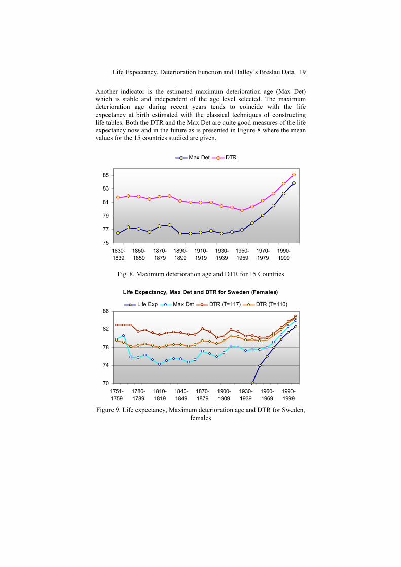
Another indicator is the estimated maximum deterioration age (Max Det)

which is stable and independent of the age level selected. The maximum

deterioration age during recent years tends to coincide with the life

expectancy at birth estimated with the classical techniques of constructing

life tables. Both the DTR and the Max Det are quite good measures of the life

expectancy now and in the future as is presented in Figure 8 where the mean

values for the 15 countries studied are given.

75

77

79

81

83

85

1830-

1839

1850-

1859

1870-

1879

1890-

1899

1910-

1919

1930-

1939

1950-

1959

1970-

1979

1990-

1999

Max Det DTR

Fig. 8. Maximum deterioration age and DTR for 15 Countries

Life Expectancy, Max Det and DTR for Sweden (Females)

70

74

78

82

86

1751-

1759

1780-

1789

1810-

1819

1840-

1849

1870-

1879

1900-

1909

1930-

1939

1960-

1969

1990-

1999

Life Exp Max Det DTR (T=117) DTR (T=110)

Figure 9. Life expectancy, Maximum deterioration age and DTR for Sweden,

females

C. H. Skiadas 20

The influence of the life level T for the estimation of life expectancy by the

DTR system in Sweden (females) is illustrated in Figure 9. Two scenarios are

selected for the estimation of the future life expectancy at birth. In the first a

T=117 year level is accepted (dark brawn line) and in the second T=110. As

it was expected the higher level for T suggests a higher level for the life

expectancy at birth via the DTR method. However, both scenarios tend to

coincide in recent years something that it is quite useful in estimating the

future trends for the life expectancy development (see Table VI). That it is

important with the DTR system is that we can construct life tables for future

dates thus doing forecasts. Instead with the Max Det we can have only an

estimate for the future levels of life expectancy at birth but not for the life

expectancy in other ages. The standard life expectancy at birth is presented

(blue line) and the Max Deterioration points are also presented (light bleu

line).

TABLE VI

Year Max Det DTR

1830-1839 76,47 81,67

1840-1849 77,26 81,98

1850-1859 77,10 81,89

1860-1869 76,65 81,51

1870-1879 77,49 81,83

1880-1889 77,59 81,96

1890-1899 76,38 81,17

1900-1909 76,39 81,03

1910-1919 76,52 80,93

1920-1929 76,76 80,98

1930-1939 76,36 80,42

1940-1949 76,57 80,26

1950-1959 76,87 79,80

1960-1969 77,90 80,39

1970-1979 79,02 81,24

1980-1989 80,50 82,31

1990-1999 82,32 83,73

2000-2007 83,81 85,03


The Halley Life Table

Edmund Halley published his famous paper in 1693. It was a pioneering

study indicating of how a scientist of a high calibre could cope to a precisely

selected data sets. Halley realized that to construct a life table from only

mortality data was fusible only on the basis of a stationary population

(Keyfitz and Caswell, 1977) by means of a population where births and

deaths are almost equal and the incoming and outgoing people are limited.

This was the case of the Breslau city in Silesia (now Wroclaw). The birth and

death data sent to Halley gave him the opportunity to construct a life table

and present his results in the paper on “An Estimate of the Degrees of the

Mortality of Mankind, drawn from curious Tables of the Births and Funerals

at the City of Breslau; with an Attempt to ascertain the Price of Annuities

upon Lives”. The same time period was also proposed a method for handling

life tables by Graunt (1662). For more information on the history and the

development of actuarial science see the related history by Haberman and

Sibbett (1995).

The purpose of this chapter is first to use the Halley’s life table data in order

to construct a mortality curve by applying a stochastic model resulting from

the first exit time theory. After applying the model and constructing the

mortality curve we find the deterioration function for the specific population

of Breslau at the years studied by Halley and thus making possible to find the

maximum deterioration age and constructing a graph for the “vitality” of the

population, a term proposed by Halley and used many years later by Strehler

and Mildvan (1960) who also suggest the term “vitality” of a person in a

stochastic modeling of the human life.

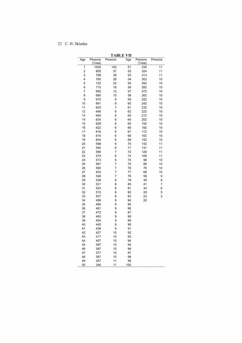
In Table VII the first two columns include the Breslau life table data from the

Halley paper whereas in the third column we have constructed the deaths per

age as the difference between two consecutive rows of the second column.

The data from the third column are inserted into our Excel program of the fist

exit time distribution function and the results are presented in Figure 10.

C. H. Skiadas 22

TABLE VII Age Persons

(Total) Persons Age Persons

(Total) Persons

1 1000 145 51 335 11

2 855 57 52 324 11

3 798 38 53 313 11

4 760 28 54 302 10

5 732 22 55 292 10

6 710 18 56 282 10

7 692 12 57 272 10

8 680 10 58 262 10

9 670 9 59 252 10

10 661 8 60 242 10

11 653 7 61 232 10

12 646 6 62 222 10

13 640 6 63 212 10

14 634 6 64 202 10

15 628 6 65 192 10

16 622 6 66 182 10

17 616 6 67 172 10

18 610 6 68 162 10

19 604 6 69 152 10

20 598 6 70 142 11

21 592 6 71 131 11

22 586 7 72 120 11

23 579 6 73 109 11

24 573 6 74 98 10

25 567 7 75 88 10

26 560 7 76 78 10

27 553 7 77 68 10

28 546 7 78 58 9

29 539 8 79 49 8

30 531 8 80 41 7

31 523 8 81 34 6

32 515 8 82 28 5

33 507 8 83 23 3

34 499 9 84 20

35 490 9 85

36 481 9 86

37 472 9 87

38 463 9 88

39 454 9 89

40 445 9 90

41 436 9 91

42 427 10 92

43 417 10 93

44 407 10 94

45 397 10 95

46 387 10 96

47 377 10 97

48 367 10 98

49 357 11 99

50 346 11 100


0,000

0,003

0,005

0,008

0,010

0,013

0,015

0,018

0,020

0 10 20 30 40 50 60 70 80 90 100 110

Data Maximum g(t)

Left Inf lection Point Right Inf lection Point Minimum

Max Deterioration Age Deterioration Function

Fig. 10. Fit curve, data plot and deterioration curve for Halley data

The estimated best fit is presented with a blue line. The parameter estimates

and the values for the characteristic points are given in the next Table VIII:

TABLE VIII

Characteristic Points of

Graph Year g(t) g'(t) Parameter

Maximum 53,3 0,011457 0 c = 2,72

Left Inflection Point 30,9 0,008182 0,0001081 b = 0,03425

Right Inflection Point 76,2 0,006412 -0,000470 l = 0,25907

Minimum 14,6 0,005679 0 k = 0,61215

Maximum Deterioration

Age 67,4

From the previous Figure and Table the estimated maximum death rate is at

the age of 53,3 years, the right inflection point is at 76,2 years, the left

inflection point is at 30,9 years and the minimum at 14,6 years. A very

important characteristic of the health state of the population is given by

C. H. Skiadas 24

estimating the age where the maximum deterioration takes place. This is

estimated at the age of 67,39 years and it is the maximum of the deterioration

function presented by a green curve in the graph.

TABLE IX

1687-1691

Data

Data

Normalised

IM Model

Estimates

Year

xK(x)

K(x)

NormalisedxK(x)

xK(x)

Normalised

Survival

curve

Life

Expectancy

145 0,1480 0,1535 0 0,0004834 0,00067177 0 0 1 79,07

57 0,0582 0,0554 1 0,0007963 0,00110653 0,0007963 1,705E-05 1 78,07

38 0,0388 0,0306 2 0,0010662 0,00148166 0,0021325 4,566E-05 0,99998295 77,07

28 0,0286 0,0202 3 0,0013116 0,00182264 0,0039348 8,4251E-05 0,99993729 76,07

22 0,0224 0,0149 4 0,0015402 0,00214027 0,0061607 0,00013191 0,99985304 75,07

18 0,0184 0,0117 5 0,0017562 0,00244044 0,0087809 0,00018802 0,99972113 74,07

12 0,0122 0,0097 6 0,0019623 0,0027268 0,0117735 0,00025209 0,99953311 73,07

10 0,0102 0,0084 7 0,0021602 0,00300181 0,0151211 0,00032377 0,99928102 72,07

9 0,0092 0,0074 8 0,0023512 0,00326723 0,0188093 0,00040274 0,99895725 71,07

8 0,0082 0,0068 9 0,0025362 0,00352437 0,0228259 0,00048874 0,99855451 70,07

7 0,0071 0,0064 10 0,002716 0,00377424 0,0271602 0,00058155 0,99806577 69,07

6 0,0061 0,0061 11 0,0028912 0,00401762 0,0318027 0,00068095 0,99748422 68,08

6 0,0061 0,0059 12 0,0030621 0,00425514 0,0367449 0,00078677 0,99680327 67,08

6 0,0061 0,0057 13 0,0032291 0,0044873 0,0419789 0,00089884 0,99601649 66,08

6 0,0061 0,0057 14 0,0033927 0,00471452 0,0474973 0,001017 0,99511765 65,09

6 0,0061 0,0057 15 0,0035529 0,00493715 0,0532931 0,0011411 0,99410065 64,09

6 0,0061 0,0057 16 0,00371 0,00515547 0,0593596 0,00127099 0,99295955 63,10

6 0,0061 0,0058 17 0,0038641 0,0053697 0,0656904 0,00140655 0,99168856 62,10

6 0,0061 0,0059 18 0,0040155 0,00558005 0,0722792 0,00154763 0,99028201 61,11

6 0,0061 0,0060 19 0,0041642 0,00578667 0,0791198 0,00169409 0,98873439 60,12

6 0,0061 0,0061 20 0,0043103 0,0059897 0,086206 0,00184582 0,98704029 59,13

7 0,0071 0,0063 21 0,0044539 0,00618923 0,0935316 0,00200268 0,98519447 58,15

6 0,0061 0,0064 22 0,004595 0,00638535 0,1010905 0,00216452 0,98319179 57,16

6 0,0061 0,0066 23 0,0047337 0,00657812 0,1088761 0,00233123 0,98102727 56,18

7 0,0071 0,0068 24 0,0048701 0,0067676 0,1168823 0,00250266 0,97869604 55,20

7 0,0071 0,0070 25 0,0050041 0,00695381 0,1251023 0,00267866 0,97619338 54,22

7 0,0071 0,0072 26 0,0051357 0,00713676 0,1335295 0,0028591 0,97351472 53,24

7 0,0071 0,0074 27 0,0052651 0,00731647 0,1421569 0,00304383 0,97065562 52,27

8 0,0082 0,0076 28 0,0053921 0,00749292 0,1509774 0,00323269 0,96761179 51,30

8 0,0082 0,0078 29 0,0055167 0,00766611 0,1599837 0,00342553 0,96437909 50,33

8 0,0082 0,0080 30 0,0056389 0,007836 0,1691681 0,00362219 0,96095356 49,37

8 0,0082 0,0082 31 0,0057588 0,00800257 0,1785229 0,00382249 0,95733137 48,40

8 0,0082 0,0084 32 0,0058762 0,00816577 0,1880398 0,00402626 0,95350888 47,45

9 0,0092 0,0086 33 0,0059912 0,00832555 0,1977106 0,00423333 0,94948262 46,49

9 0,0092 0,0088 34 0,0061037 0,00848187 0,2075264 0,00444351 0,94524929 45,54

9 0,0092 0,0091 35 0,0062137 0,00863466 0,2174784 0,0046566 0,94080578 44,60

9 0,0092 0,0093 36 0,006321 0,00878386 0,2275573 0,0048724 0,93614918 43,66

9 0,0092 0,0095 37 0,0064258 0,00892941 0,2377536 0,00509072 0,93127678 42,72

9 0,0092 0,0097 38 0,0065278 0,00907122 0,2480573 0,00531134 0,92618605 41,79

9 0,0092 0,0099 39 0,0066271 0,00920923 0,2584584 0,00553405 0,92087471 40,86

9 0,0092 0,0101 40 0,0067237 0,00934336 0,2689465 0,00575862 0,91534066 39,94

10 0,0102 0,0102 41 0,0068173 0,00947353 0,2795107 0,00598482 0,90958204 39,03

10 0,0102 0,0104 42 0,0069081 0,00959966 0,2901403 0,00621242 0,90359722 38,12

10 0,0102 0,0106 43 0,0069959 0,00972167 0,3008238 0,00644117 0,89738481 37,22

10 0,0102 0,0107 44 0,0070807 0,00983948 0,3115499 0,00667083 0,89094364 36,32

10 0,0102 0,0109 45 0,0071624 0,009953 0,3223068 0,00690116 0,88427281 35,43

10 0,0102 0,0110 46 0,0072409 0,01006216 0,3330826 0,00713189 0,87737165 34,54

10 0,0102 0,0111 47 0,0073163 0,01016688 0,3438651 0,00736276 0,87023976 33,67

11 0,0112 0,0112 48 0,0073884 0,01026706 0,3546421 0,00759351 0,862877 32,79

11 0,0112 0,0113 49 0,0074572 0,01036265 0,3654011 0,00782388 0,85528349 31,93

11 0,0112 0,0114 50 0,0075226 0,01045357 0,3761295 0,0080536 0,84745961 31,08

DTR System (Halley, Breslaw Data)


11 0,0112 0,0114 51 0,0075846 0,01053974 0,3868146 0,00828238 0,83940601 30,23

11 0,0112 0,0114 52 0,0076431 0,0106211 0,3974436 0,00850997 0,83112363 29,39

10 0,0102 0,0115 53 0,0076982 0,01069758 0,4080037 0,00873608 0,82261366 28,56

10 0,0102 0,0115 54 0,0077497 0,01076912 0,4184821 0,00896044 0,81387758 27,74

10 0,0102 0,0114 55 0,0077976 0,01083568 0,4288659 0,00918278 0,80491714 26,92

10 0,0102 0,0114 56 0,0078418 0,01089719 0,4391425 0,00940282 0,79573437 26,12

10 0,0102 0,0113 57 0,0078824 0,01095362 0,449299 0,00962028 0,78633155 25,32

10 0,0102 0,0112 58 0,0079194 0,01100493 0,459323 0,00983491 0,77671127 24,54

10 0,0102 0,0111 59 0,0079526 0,01105109 0,4692019 0,01004644 0,76687635 23,76

10 0,0102 0,0110 60 0,0079821 0,01109206 0,4789236 0,0102546 0,75682991 22,99

10 0,0102 0,0108 61 0,0080078 0,01112783 0,4884759 0,01045913 0,74657531 22,23

10 0,0102 0,0107 62 0,0080298 0,01115839 0,4978472 0,01065979 0,73611618 21,49

10 0,0102 0,0105 63 0,008048 0,01118373 0,5070259 0,01085632 0,7254564 20,75

10 0,0102 0,0103 64 0,0080625 0,01120386 0,5160009 0,01104849 0,71460008 20,03

10 0,0102 0,0100 65 0,0080733 0,01121878 0,5247614 0,01123607 0,70355158 19,31

10 0,0102 0,0098 66 0,0080803 0,01122851 0,5332968 0,01141883 0,69231552 18,61

10 0,0102 0,0095 67 0,0080835 0,01123308 0,5415973 0,01159655 0,68089669 17,92

10 0,0102 0,0092 68 0,0080831 0,01123251 0,5496531 0,01176904 0,66930014 17,24

11 0,0112 0,0089 69 0,0080791 0,01122686 0,5574552 0,0119361 0,6575311 16,57

11 0,0112 0,0086 70 0,0080714 0,01121615 0,5649951 0,01209754 0,645595 15,91

11 0,0112 0,0083 71 0,0080601 0,01120046 0,5722645 0,01225319 0,63349746 15,26

11 0,0112 0,0079 72 0,0080452 0,01117983 0,579256 0,01240289 0,62124426 14,63

10 0,0102 0,0076 73 0,0080269 0,01115435 0,5859626 0,01254649 0,60884137 14,01

10 0,0102 0,0072 74 0,0080051 0,01112408 0,5923778 0,01268385 0,59629488 13,40

10 0,0102 0,0069 75 0,0079799 0,01108912 0,5984959 0,01281485 0,58361102 12,80

10 0,0102 0,0065 76 0,0079515 0,01104955 0,6043116 0,01293938 0,57079617 12,22

9 0,0092 0,0061 77 0,0079197 0,01100547 0,6098205 0,01305733 0,55785679 11,65

8 0,0082 0,0057 78 0,0078849 0,01095698 0,6150184 0,01316863 0,54479946 11,09

7 0,0071 0,0054 79 0,0078469 0,01090418 0,619902 0,0132732 0,53163083 10,55

6 0,0061 0,0050 80 0,0078059 0,01084721 0,6244688 0,01337098 0,51835763 10,01

5 0,0051 0,0047 81 0,0077619 0,01078616 0,6287165 0,01346193 0,50498666 9,50

3 0,0031 0,0043 82 0,0077152 0,01072118 0,6326437 0,01354602 0,49152473 8,99

0 0,0000 0,0040 83 0,0076657 0,01065238 0,6362496 0,01362323 0,47797871 8,50

0 0,0000 0,0037 84 0,0076135 0,0105799 0,6395341 0,01369355 0,46435548 8,02

0 0,0000 0,0033 85 0,0075588 0,01050388 0,6424973 0,013757 0,45066193 7,56

0 0,0000 0,0030 86 0,0075016 0,01042445 0,6451404 0,01381359 0,43690493 7,11

0 0,0000 0,0028 87 0,0074421 0,01034175 0,6474649 0,01386337 0,42309133 6,67

0 0,0000 0,0025 88 0,0073804 0,01025594 0,6494729 0,01390636 0,40922797 6,25

0 0,0000 0,0022 89 0,0073165 0,01016716 0,651167 0,01394263 0,39532161 5,84

0 0,0000 0,0020 90 0,0072506 0,01007555 0,6525504 0,01397226 0,38137897 5,44

0 0,0000 0,0018 91 0,0071827 0,00998127 0,6536268 0,0139953 0,36740672 5,06

0 0,0000 0,0016 92 0,007113 0,00988446 0,6544002 0,01401186 0,35341142 4,69

0 0,0000 0,0014 93 0,0070417 0,00978527 0,6548754 0,01402204 0,33939955 4,34

0 0,0000 0,0012 94 0,0069687 0,00968386 0,6550573 0,01402593 0,32537751 4,00

0 0,0000 0,0010 95 0,0068942 0,00958038 0,6549513 0,01402366 0,31135158 3,68

0 0,0000 0,0009 96 0,0068184 0,00947496 0,6545632 0,01401535 0,29732792 3,36

0 0,0000 0,0008 97 0,0067412 0,00936777 0,6538991 0,01400113 0,28331257 3,07

0 0,0000 0,0007 98 0,0066629 0,00925894 0,6529656 0,01398114 0,26931143 2,78

0 0,0000 0,0006 99 0,0065835 0,00914863 0,6517693 0,01395553 0,25533029 2,51

0 0,0000 0,0005 100 0,0065032 0,00903696 0,6503172 0,01392444 0,24137476 2,26

0 0,0000 0,0004 101 0,0064219 0,00892409 0,6486166 0,01388802 0,22745032 2,02

0 0,0000 0,0003 102 0,0063399 0,00881014 0,6466749 0,01384645 0,2135623 1,79

0 0,0000 0,0003 103 0,0062573 0,00869526 0,6444997 0,01379988 0,19971585 1,58

0 0,0000 0,0002 104 0,006174 0,00857958 0,6420989 0,01374847 0,18591597 1,38

0 0,0000 0,0002 105 0,0060903 0,00846321 0,6394804 0,0136924 0,1721675 1,19

0 0,0000 0,0001 106 0,0060062 0,00834629 0,636652 0,01363184 0,1584751 1,02

0 0,0000 0,0001 107 0,0059217 0,00822894 0,6336221 0,01356697 0,14484325 0,86

0 0,0000 0,0001 108 0,005837 0,00811127 0,6303986 0,01349795 0,13127629 0,71

0 0,0000 0,0001 109 0,0057522 0,00799339 0,6269897 0,01342496 0,11777834 0,58

0 0,0000 0,0001 110 0,0056673 0,00787542 0,6234038 0,01334817 0,10435338 0,47

0 0,0000 0,0000 111 0,0055824 0,00775747 0,6196488 0,01326777 0,09100521 0,36

0 0,0000 0,0000 112 0,0054976 0,00763962 0,615733 0,01318393 0,07773744 0,27

0 0,0000 0,0000 113 0,005413 0,00752198 0,6116645 0,01309682 0,06455351 0,19

0 0,0000 0,0000 114 0,0053285 0,00740464 0,6074512 0,0130066 0,05145669 0,13

0 0,0000 0,0000 115 0,0052444 0,00728769 0,6031012 0,01291346 0,03845009 0,08

0 0,0000 0,0000 116 0,0051605 0,00717121 0,5986224 0,01281756 0,02553663 0,04

0 0,0000 0,0000 117 0,0050771 0,00705528 0,5940223 0,01271907 0,01271907 0,01

1,0000 0,7196193 1 46,70 1 79,07

C. H. Skiadas 26

The DTR system as presented earlier provides the last Life Table IX from

which we can find a future life expectancy based on the deterioration

function. The surprising result is that the estimated life expectancy is quite

close to the values for Germany from 2000-2008 and higher than the related

values for Poland (2005-2009) as provided by the Human Mortality

Database. The estimates are presented in the next Figure 11 along with the

estimates for the life expectancy estimated by the Breslau data (see the green

line in the graph).

Life Expectancy

0

10

20

30

40

50

60

70

80

90

0 20 40 60 80 100 120

Halley Data Det_Method Poland 2005-2009

Haley Data Life_Exp Germany 2000-2008

Fig. 11. Life expectancy curves for Breslau data

Illustration of the development of the maximum deterioration age from the

Halley days until today is given in Figure 12. The maximum deterioration

age for the Breslau data (1687-1691) was 67,39 years and continued to

increase by 4,75 years per century.


Maximum Deterioration Age

65

70

75

80

85

90

1687-

1691

1710-

1719

1740-

1749

1770-

1779

1800-

1809

1830-

1839

1860-

1869

1890-

1899

1920-

1929

1950-

1959

1980-

1989

Males Females Both-Mean Projection

Fig. 12. Maximum Deterioration Age for various time periods

The Program

A computer program (IM-model-DTR-Life_Tables) was developed to be able

to make the necessary computations related to this paper. Furthermore the

program estimates the life expectancy tables by based on the mortality and

population data. The life expectancy is also estimated by based on the fitting

curve thus making more accurate the related estimations. The program and

the related theory can be found in the website: http://www.cmsim.net. The

program is developed in Excel 2003 and it is very easy to use without any

special tool.

Conclusions

We have developed and applied a new theoretical framework for analyzing

mortality data. The work starting several years ago was based on the

stochastic theory and the derivation of a first exit time distribution function

suitable for expressing the human mortality. Furthermore we have explored

on how we could model the so-called “vitality” of a person or the opposite

term the deterioration of an organism and to provide a function, the

deterioration function, which could be useful for sociologists, police makers

and the insurance people in making their estimates and plan the future.

Acknowledgments

The data used can be downloaded from the Human Mortality Database at:

http://www.mortality.org or from the statistical year-books of the countries

studied.

C. H. Skiadas 28

References

A. Economos, A non-Gompertzian paradigm for mortality kinetics of

metazoan animals and failure kinetics of manufactured products. Age,

vol.2, 74-76 (1979).

A. Economos, Kinetics of metazoan mortality. J. Social Biol. Struct., 3, 317-

329 (1980).

B. Gompertz, On the nature of the function expressive of the law of human

mortality, and on the mode of determining the value of life contingencies,

Philosophical Transactions of the Royal Society of London A 115, 513-

585 (1825).

J. Graunt, Natural and Political Observations Made upon the Bills of

Mortality, First Edition, 1662; Fifth Edition (1676).

M. Greenwood and J. O. Irwin, The biostatistics of senility, Human Biology,

vol.11, 1-23 (1939).

S. Haberman and T. A. Sibbett, History of Actuarial Science, London, UK:

William Pickering, (1995).

E. Halley, An Estimate of the Degrees of Mortality of Mankind, Drawn from

the Curious Tables of the Births and Funerals at the City of Breslau, with

an Attempt to Ascertain the Price of Annuities upon Lives, Philosophical

Transactions, Volume 17, pp. 596-610 (1693).

L. M. A. Heligman and J. H. Pollard, The Age Pattern of mortality, Journal

of the Institute of Actuaries 107, part 1, 49-82 (1980).

J. Janssen and C. H. Skiadas, Dynamic modelling of life-table data, Applied

Stochastic Models and Data Analysis, 11, 1, 35-49 (1995).

N. Keyfitz and H. Caswell, Applied Mathematical Demography, 3rd ed.,

Springer (2005).

R. D. Lee and L. R. Carter, Modelling and forecasting U.S. mortality. J.

Amer. Statist. Assoc. 87 (14), 659–675 (1992).

W. M. Makeham, On the Law of Mortality and the Construction of Annuity

Tables, J. Inst. Act. and Assur. Mag. 8, 301-310, (1860).

C. H. Skiadas and C. Skiadas, A modeling approach to life table data, in

Recent Advances in Stochastic Modeling and Data Analysis, C. H.

Skiadas, Ed. (World Scientific, Singapore), 350–359 (2007).

C. H. Skiadas, C. Skiadas, Comparing the Gompertz Type Models with a

First Passage Time Density Model, in Advances in Data Analysis, C. H.

Skiadas Ed. (Springer/Birkhauser, Boston), 203-209 (2010).

C. Skiadas and C. H. Skiadas, Development, Simulation and Application of

First Exit Time Densities to Life Table Data, Communications in

Statistics 39, 444-451 (2010).

C. H. Skiadas and C. Skiadas, Exploring life expectancy limits: First exit

time modelling, parameter analysis and forecasts, in Chaos Theory:

Modeling, Simulation and Applications, C. H. Skiadas, I. Dimotikalis and

C. Skiadas, Eds. (World Scientific, Singapore), 357–368 (2011).

B. L. Strehler and A.S. Mildvan, General theory of mortality and aging,

Science 132, 14-21 (1960).

a life expectancy study based on the deterioration - cmsim.net

Documents