A linear energy stable scheme for a thin film modelwithout slope selection

Wenbin ChenSchool of Mathematics, Fudan University

Shanghai, China 200433and

Sidafa CondeDepartment of Mathematics, U. Massachusetts, Dartmouth

North Dartmouth, MA 02747-2300and

Cheng Wang∗

Department of Mathematics, U. Massachusetts, DartmouthNorth Dartmouth, MA 02747-2300

andXiaoming Wang

Department of Mathematics, Florida State U.Tallahassee, FL 32306-4510

andSteven M. Wise

Department of Mathematics, U. of TennesseeKnoxville, TN 37996-1300

November 29, 2010

Abstract

We present a linear numerical scheme for a model of epitaxial thin film growth with-out slope selection. The PDE, which is a nonlinear, fourth-order parabolic equation, isthe L2 gradient flow of the energy

∫Ω

(−1

2 ln(1 + |∇φ|2

)+ ε2

2 |∆φ(x)|2)

dx. The ideaof convex-concave decomposition of the energy functional is applied, which results ina non-increasing energy property at the numerical level. The particular decompositionused here places the nonlinear term in the concave part of the energy, in contrast to aprevious convexity splitting scheme. As a result, the numerical scheme is fully linear

∗Corresponding author, cwang1@umassd.edu

1

at each time step and unconditionally solvable. Collocation Fourier spectral differen-tiation is used in the spatial discretization, and the unconditional energy stability isestablished in the fully discrete setting using a detailed energy estimate. We presentthe numerical simulation results of the physical model with a sequence of ε values rang-ing from 0.01 to 0.1. In particular, the long time simulations show the −log(t) decaylaw for the energy and the t1/2 growth law for the surface roughness, in agreement withtheoretical analysis and experimental/numerical observations in earlier works.

1 Introduction

In this article we consider an efficient numerical scheme for a continuum (2+1)-dimensionalheight-function model of epitaxial thin film growth. (See the review [8] for the recent historyof such models of thin film growth.) The equation is the gradient flow associated with thefollowing energy functional

E(φ) :=

∫Ω

(−1

2ln(1 + |∇φ|2

)+ε2

2|∆φ|2

)dx , (1)

where Ω = [0, Lx]× [0, Ly], φ : Ω→ R is a periodic height function, and ε is a constant. Wenote that the first term, a nonlinear term, represents the Ehrlich-Schwoebel effect, accordingto which adatoms (absorbed atoms) must overcome a higher energy barrier to stick to astep from an upper rather than from a lower terrace [6, 16, 19]. This results in an uphillatom current and the steepening of mounds in the film. The second term, the linear term,represents the isotropic (i.e., random) surface diffusion effect [16, 18]. To clearly distinguishthe nonlinear Ehrlich-Schwoebel term from the linear surface diffusion term, we write

EES(φ) :=

∫Ω

FES (∇φ) dx , FES(y) := −1

2ln(1 + |y|2

), (2)

where y ∈ R2 and |y| =√y2

1 + y22. Hence, E(φ) = EES(φ) + ε2

2‖∆φ‖2 where ‖ · ‖ denotes

the L2 norm (rms).The use of the nonlinear Ehrlich-Schwoebel term of the form (2) appears to have orig-

inated in the work [12]. Note that FES : R2 → R is bounded above by 0 and unboundedbelow. In fact FES → −∞ as |y| → ∞. Furthermore, FES has no relative minima, whichimplies that there are no energetically favored values for |∇φ|. Physically this means thatthere is no slope selection mechanism, at least from an energetic point of view, that couldset a preferred slope of the height function φ. See the relevant discussions in [13, 14, 16, 17].

The chemical potential is defined to be the variational derivative of the energy (1), i.e.,

µ := δφE = ∇ ·(

∇φ1 + |∇φ|2

)+ ε2∆2φ . (3)

Here we consider the gradient flow of the form

∂tφ = −µ = −∇ ·(

∇φ1 + |∇φ|2

)− ε2∆2φ , (4)

2

where the boundary conditions for the height function φ are taken to be periodic in bothspatial directions. This equation may be rewritten in the form

∂tφ = ∇ ·(|∇φ|2

1 + |∇φ|2∇φ)−∆φ− ε2∆2φ . (5)

In the small-slope regime, where |∇φ|2 1, (5) may be replaced by

∂tφ = ∇ ·(|∇φ|2∇φ

)−∆φ− ε2∆2φ , (6)

which we refer to as the slope-selection equation [13, 14, 16]. Solutions to Eq. (6), unlikethose of Eq. (4), exhibit pyramidal structures, where the faces of the pyramids have slopes|∇φ| ≈ 1. Solutions to the no-slope-selection equation (4), on the other hand, exhibit mound-like structures, the slopes of which (on an infinite domain) may grow unbounded [16, 23].Note that solutions of (6) and (4) have up-down symmetry, in an average sense. In otherwords, there is no way to distinguish a hill from a valley.

Typically one is interested in the how certain quantities associated with the solutions to(4) and (6) scale with time, where ε is assumed small. The physically interesting quantitiesthat may be obtained from the solutions of these equations are the surface roughness, definedas

w(t) =

√1

|Ω|

∫Ω

∣∣∣φ(x, t)− φ(t)∣∣∣2dx , (7)

the characteristic pyramid/mound size, denoted λ(t), and the energy. For the slope-selectionequation (6) numerical simulations and rigorous (as well as non-rigorous) scaling argumentshave demonstrated that w ∼ O

(t1/3), λ(t) ∼ O

(t1/3), and E ∼ O

(t−1/3

). Likewise,

for the no-slope-selection equation (4), one obtains w ∼ O(t1/2), λ(t) ∼ O

(t1/4), and

E ∼ O (− ln(t)). Observe that for the no-slope-selection equation (4), the average moundheight (measured by the roughness) grows faster then the mound width (measured by λ),which is expected because there is no preferred slope of the height function φ. Also, note thatin the rigorous setting, for example [13, 14, 17], one can only (at best) obtain lower boundsfor the energy dissipation and, conversely, upper bounds for the roughness growth. However,the rates quoted as the upper or lower bounds are typically observed in some average sensein the numerical computations and are therefore taken as the values of the average ratesthemselves.

Practically speaking, predicting these scaling laws numerically is quite challenging, sincethey require very long simulation times. Moreover, these laws are expected to break downthe closer one gets to the saturation time, which for the no-slope-selection equation (4)scales like O (ε2). (See Figs. 2, 4, and 5 and the related discussion in Sec. 4. Also, seeFig. 1 of [17].) But the solution behavior is ill-understood, computationally and rigorously,near the saturation time. To adequately capture the full range of coarsening behaviors,numerical simulations for the coarsening process — which for small ε involve small spatialresolution — require short-, intermediate-, and long-time accuracy and stability. In thispaper, we build on our previous work [23] by introducing an efficient linear, unconditionallystable, unconditionally solvable scheme for approximating solutions to the no-slope-selectionequation (4). The scheme is based on a convexity splitting of the energy (1) into a purelyconvex part and a purely concave part.

3

The introduction of convexity splitting schemes is generally attributed to Eyre [9]. Tonumerically solve the Cahn-Hilliard and Allen-Cahn equations, Eyre proposed to decomposethe Cahn-Hilliard energy, ECH(φ) = 1

4‖φ‖4

L4 − 12‖φ‖2

L2 + ε2

2‖∇φ‖2

L2 , into a convex part anda concave part. In the convexity splitting scheme, one treats the terms of the variationalderivative implicitly or explicitly according to whether the terms correspond to the convexor concave parts of the energy, respectively. For the canonical decomposition of the Cahn-Hilliard energy above, one obtains the convexity splitting approximation

µk+1 =(φk+1

)3 − φk − ε2∆φk+1 , (8)

where µ = δφECH is the chemical potential relative to the energy. Eyre’s convex-splitting

scheme is first-order accurate in time, unconditionally uniquely solvable, and unconditionallyenergy stable in the sense that the energy is monotonically non-increasing in (discrete) time,regardless of the time step size. Such unconditionally stable schemes are highly desirablewith regard to long time numerical simulation, especially for coarsening processes that requireincreasingly larger time step sizes for efficient computation.

We extended Eyre’s convexity splitting idea in [23] to deal with terms in the chemicalpotential that are nonlinear in the gradients of φ. In particular, we applied the convexitysplitting methodology to develop schemes for both the slope-selection (6) and no-slope-selection (4) equations. In [23], our scheme for the latter equation was

φn+11 − φn1k

= −µk+1 = ∇ ·

(∇φn+1

1

∣∣∇φn+11

∣∣21 +

∣∣∇φn+11

∣∣2)−∆φn1 − ε2∆2φn+1

1 . (9)

This is based on the energy splitting

E(φ) =

∫Ω

(1

2

(|∇φ|2 − ln

(1 + |∇φ|2

))+ε2

2|∆φ(x)|2

)dx−

∫Ω

1

2|∇φ|2 dx , (10)

where it may be observed that the part associated with the first integral is convex, and thepart associated with the second is concave. The primary drawback of the method (9) is thatit is nonlinear. However, it may be observed that solving this scheme is equivalent to solvinga strictly convex, coercive optimization problem. This is a general feature of convexitysplitting schemes [22, 23]. In [23] we used an efficient nonlinear conjugate gradient methodto solve (9). This was a natural choice because of the convex nature of the problem at theimplicit time level.

Other schemes have been developed for the no-slope-selection equation (4). For instanceLi and Liu developed a spectral method in [16]. See also the computational results in [12].However, besides our own work in [23], to our knowledge no one has analyzed any schemesfor the no-slope-selection equation (4).

The main contribution of this manuscript is an alternate convex-concave decompositionof the energy (1) associated with the epitaxy thin film model without slope selection. It isobserved that the nonlinear term ln

(1 + |∇φ|2

)is bounded by |∇φ|2 in functional norms.

Thus, instead of placing the nonlinear term in the convex part, we may — by appropriatelyadding and subtracting the term 1

2‖∇φ‖2 in the energy — place the nonlinear part in the

concave portion of the energy. As a result, the nonlinear term is treated explicitly in theconvex splitting scheme; the scheme then becomes purely linear! More importantly, the

4

linear operator involved in the scheme, which is positive and has constant coefficients, canbe efficiently inverted by FFT or other existing fast linear solvers. This gives rise to a schemethat is vastly more efficient than the nonlinear counterpart (9) developed in [23]. In addition,this purely linear scheme also preserves the unconditional energy stability that was enjoyedby the nonlinear scheme, due to its convex splitting nature.

We will show that this energy dissipation property is valid for both the semi-discretescheme (time discrete, space continuous) and the fully discrete scheme. In this paper, weuse collocation Fourier spectral differentiation (in both the first, second and fourth orderderivatives) to effect spatial discretization. Another observation of the energy stability isthat it can be derived by using an energy estimate other than the general convexity analysiswe provided in [23]. Therefore, we could apply integration by parts in the collocation Fourierspectral differentiation and carry out the energy estimate at the discrete level. That in turnleads to unconditional stability with respect to the discrete energy.

The rest of the manuscript is organized as follows. In Sec. 2 we recall the energy stabilityresult for general convex splitting schemes, present the alternate convex-concave decompo-sition of the energy (1), and formulate the corresponding purely linear numerical scheme.We show that the unconditional energy stability of the scheme may be derived by usingeither the general analysis from [23], or more directly using an energy estimate. In Sec. 3 wepresent the fully discrete scheme, where Fourier spectral differentiation is utilized in space.The energy stability will be established at the fully discrete level, based on integration byparts in Fourier space. In Sec. 4 we present some numerical simulation results. We offer ourconcluding remarks in Sec. 5.

2 The Numerical Scheme

2.1 Energy Stability of Convex Splitting Schemes

The natural function space for our problem is the subspace of H2(Ω) whose functions areperiodic and have zero average, which we denote by H2

per(Ω). To begin, we consider a generalenergy functional of the form

E(φ) = EES(φ) +ε2

2‖∆φ‖2 , (11)

for all φ ∈ H2per(Ω), where

EES(φ) =

∫Ω

FES (∇φ) dx , (12)

and FES : R2 → R is twice differentiable. We suppose that this FES can be decomposed(non-uniquely) into convex and concave terms — respectively, contractive and expansiveterms in the language of Eyre [9] — in the sense that

FES (y) = FESc (y)− FES

e (y) , (13)

where D2yF

ESc , D2

yFESe ≥ 0. Subordinate to this decomposition of the energy density F we

define the Ehrlich-Schwoebel-type energies

EESc (φ) :=

∫Ω

FESc (∇xφ) dx , EES

e (φ) :=

∫Ω

FESe (∇xφ) dx , (14)

5

so that EES(φ) = EESc (φ)− EES

e (φ). The associated gradient flow is given by

∂tφ = −δφEESc + δφE

ESe − ε2∆2φ , (15)

where δφ is the variational derivative with respect to φ. The corresponding convex splittingnumerical scheme for the gradient flow (15) with time step size k > 0 can be written as

φn+1 − φn

k= −δφEES

c

(φn+1

)+ δφE

ESe (φn)− ε2∆2φn+1

= ∇x · ∇yFESc

(∇xφ

n+1)−∇x · ∇yF

ESe (∇xφ

n)− ε2∆2φn+1 . (16)

Notice that this scheme in not uniquely defined, since the convex-concave splitting is notunique in general. This subtle fact will lead to the key observation of this article.

The following result guarantees the unconditional energy stability and convergence forthe convex splitting scheme (16). Related results can also be found in [22].

Theorem 1 (Thm. 1 [23]). Assume that the energy functional (11) is twice functional dif-ferentiable on H2

per(Ω), and FES (y), ∇yFES (y) grow at most polynomially in y. Then the

scheme given by (16) for the gradient system (15) satisfying the convexity splitting (13) iswell-posed, with the solution given by the unique minimizer of the following modified energyfunctional:

Escheme(φ) :=ε2

2‖∆φ‖2 + EES

c (φ) +1

2k‖φ‖2 −

∫Ω

(δφE

ESe (φn) +

1

kφn)φ dx . (17)

Moreover, the energy is a non-increasing function of time, i.e., we have

Escheme(φn+1) ≤ Escheme(φ

n)− 1

k

∥∥φn+1 − φn∥∥2 − ε2

2

∥∥∆(φn+1 − φn

)∥∥2, ∀ k > 0 . (18)

And, the solution to the scheme (16) converges to the solution of the thin film epitaxy model(15) at vanishing time step size (k → 0) on any finite time interval.

As we have already mentioned, for the thin film model (4), we previously [23] proposeda convexity splitting of the form EES(φ) = EES

c (φ)− EESe (φ), where

EESc (φ) =

∫Ω

1

2

|∇φ|2 − ln

(1 + |∇φ|2

)dx , EES

e (φ) =

∫Ω

1

2|∇φ|2 dx . (19)

The convex splitting scheme for the no-slope-selection equation (4) subordinate to this split-ting is then given in (9). The energy stability of (9) is a corollary of Theorem 1. See(18).

2.2 A Linear Convex Splitting Scheme

The main contribution of this article is an alternate convexity splitting of the Ehrlich-Schwoebel energy EES for the thin film model without slope selection. Specifically, considerthe splitting EES(φ) = EES

c (φ)− EESe (φ), where

EESc (φ) =

∫Ω

1

2|∇φ|2 dx , EES

e (φ) =

∫Ω

1

2

|∇φ|2 + ln

(1 + |∇φ|2

)dx . (20)

6

The convexity of EESc is obvious, and the convexity of EES

e comes from the convexity of thefollowing function

G(y) =1

2

|y|2 + ln

(1 + |y|2

). (21)

The corresponding convex splitting numerical scheme is given by

φn+1 − φn

k= ∆φn+1 −∇ ·

(∇φn

1 + |∇φn|2

)−∆φn − ε2∆2φn+1 . (22)

Of course, the proposed scheme (22) is purely linear due to the explicit treatment of thenonlinear term. It can be reformulated as(

1

kI −∆ + ε2∆2

)φn+1 = fn :=

φn

k−∇ ·

(∇φn

1 + |∇φn|2

)−∆φn. (23)

Even without Thm 1, it may observed that the scheme is unconditionally uniquely solvable.In fact, a simple calculation reveals that all the eigenvalues of the operator on the left handside of (23) are positive. The main advantage of (22), over any other nonlinear scheme, isthat spectral and fast elliptic solvers are directly applicable. This fact shows the importanceof the alternate energy decomposition (20), where the nonlinear part of the energy can betransferred to the concave (expansive) part of the energy. And, according to the analysisin [22, 23], the concave part of the energy should always be treated explicitly in the numericalscheme.

2.3 Energy Stability via a Direct Proof

Because our linear scheme (22) is derived from a convexity splitting, namely, (20), theunconditional energy stability (18) and finite time convergence are guaranteed by Thm. 1.However, in the following we show the energy stability directly, without appealing to thegeneral result in Thm. 1.

Lemma 1. Numerical solutions of (22) satisfy the energy dissipation inequality (18). Inother words, (22) is an energy stable scheme.

Proof. Taking L2 inner product of (22) with φn+1 − φn yields

−1

k

∥∥φn+1 − φn∥∥2

=

(φn+1 − φn,∇ ·

(∇φn

1 + |∇φn|2

))+(φn+1 − φn,∆φn

)−(φn+1 − φn,∆φn+1

)+ ε2

(φn+1 − φn,∆2φn+1

). (24)

For the linear terms, integration by parts can be applied and the following equalities arestandard:(

φn+1 − φn,∆φn −∆φn+1)

=∥∥∇ (φn+1 − φn

)∥∥2, (25)(

φn+1 − φn,∆2φn+1)

=1

2

(∥∥∆φn+1∥∥2 − ‖∆φn‖2

)+

1

2

∥∥∆(φn+1 − φn

)∥∥2. (26)

For the nonlinear term, we also start with an integration by parts:

I :=

(φn+1 − φn,∇ ·

(∇φn

1 + |∇φn|2

))= −

(∇φn+1 −∇φn, ∇φn

1 + |∇φn|2

). (27)

7

A careful calculation shows that

− ln(1 + |∇φn+1|2

)+ ln

(1 + |∇φn|2

)= ln

(1 + |∇φn|2

1 + |∇φn+1|2

)= ln

(1 +|∇φn|2 − |∇φn+1|2

1 + |∇φn+1|2

)≤ |∇φn|2 − |∇φn+1|2

1 + |∇φn+1|2, (28)

where the last step follows from the inequality

ln(1 + r) ≤ r , ∀ r > −1 . (29)

Note that inequality (28) is a point-wise estimate, and it implies that

EES(φn+1)− EES(φn) =

∫Ω

(−1

2ln(1 + |∇φn+1|2

)+

1

2ln(1 + |∇φn|2

))dx

≤ 1

2

∫Ω

|∇φn|2 − |∇φn+1|2

1 + |∇φn+1|2dx

=

∫Ω

−12

(∇φn+1 +∇φn) · (∇φn+1 −∇φn)

1 + |∇φn+1|2dx . (30)

The combination of (27) and (30) indicates that

I −[EES

(φn+1

)− EES (φn)

]≥∫

Ω

(− (∇φn+1 −∇φn) · ∇φn

1 + |∇φn|2+

12

(∇φn+1 +∇φn) · (∇φn+1 −∇φn)

1 + |∇φn+1|2

)dx . (31)

Meanwhile, a careful calculation reveals the following point-wise estimate:

− (∇φn+1 −∇φn) · ∇φn

1 + |∇φn|2+

12

(∇φn+1 +∇φn) · (∇φn+1 −∇φn)

1 + |∇φn+1|2≥ −

∣∣∇φn+1 −∇φn∣∣2 . (32)

Its substitution into (31) gives

I −[ENS

(φn+1

)− EES (φn)

]≥ −

∥∥∇ (φn+1 − φn)∥∥2

. (33)

Finally, combining (24) – (26) and (33) results in

EES(φn+1

)− EES (φn) +

ε2

2

(‖∆φn+1‖2 − ‖∆φn‖2

)≤ −ε

2

2‖∆(φn+1 − φn

)‖2

−1

k‖φn+1 − φn‖2 , (34)

which is equivalent to (18) since E(φ) = EES(φ) + ε2

2‖∆φ‖2.

8

3 Fully Discrete Linear Scheme

3.1 Definition and Unique Solvability

Since the boundary conditions are periodic and the differential operator in (23) is linearwith constant coefficients, we use collocation Fourier spectral differentiation to effect spatialdiscretization. Assume that Lx = Nx ·hx and Ly = Ny ·hy, for some mesh sizes hx, hy > 0 andsome positive integers Nx and Ny. For simplicity of presentation, we use a square domain,i.e., Lx = Ly = L, and a uniform mesh size hx = hy = h, Nx = Ny = N is taken. Allthe variables are evaluated at the regular numerical grid (xi, yj), with xi = ih, yj = jh,0 ≤ i, j ≤ N .

For a periodic function f over the given 2D numerical grid, assume its discrete Fourierexpansion is given by

fi,j =

N/2∑k,l=−N/2+1

fk,l exp

(2kπixiL

)exp

(2lπiyjL

). (35)

Then the Fourier spectral approximations to the first and second order partial derivativesare given by

(DNxf)i,j =

N/2∑k,l=−N/2+1

(2kπi

L

)fk,l exp

(2kπixiL

)exp

(2lπiyjL

), (36)

(DNyf)i,j =

N/2∑k,l=−N/2+1

(2lπi

L

)fk,l exp

(2lπixiL

)exp

(2lπiyjL

), (37)

(D2Nxf

)i,j

=

N/2∑k,l=−N/2+1

(−4π2k2

L2

)fk,l exp

(2kπixiL

)exp

(2lπiyjL

), (38)

(D2Nyf

)i,j

=

N/2∑k,l=−N/2+1

(−4π2l2

L2

)fk,l exp

(2kπixiL

)exp

(2lπiyjL

). (39)

The discrete Laplacian, gradient and divergence operators become

∆Nf = D2Nxf +D2

Nyf , ∇Nf =

(DNxfDNyf

), ∇N ·

(f1

f2

)= DNxf1 +DNyf2 , (40)

at the point-wise level. The fully discrete scheme is formulated as

φn+1 − φn

k= −∇N ·

(∇Nφ

n

1 + |∇Nφn|2

)−∆Nφ

n + ∆Nφn+1 − ε2∆2

Nφn+1 . (41)

It is straightforward to show that the fully discrete scheme (41) is unconditionally uniquelysolvable. To see this consider a reformulation of (41) similar to (23):(

1

kI −∆N + ε2∆2

N

)φn+1 = fn :=

φn

k−∇N ·

(∇Nφ

n

1 + |∇Nφn|2

)−∆Nφ

n . (42)

9

Now, for each eigenfunction exp(

2kπixi

L

)exp

(2lπiyj

L

), −N

2+ 1 ≤ k, l ≤ N

2, the corresponding

eigenvalue for the operator on the left hand side of (42) is precisely

λk,l :=1

k− (λk + λl) + ε2 (λk + λl)

2 , (43)

where

λk = −4π2k2

L2x

, λl = −4π2l2

L2y

. (44)

Consequently, λk,l > 0, which implies the unique unconditional solvability of the fully discretescheme (41). Naturally, the FFT can be very efficiently utilized to obtain numerical solutions.

Remark 1. In this work, we use a collocation Fourier spectral differentiation other thanthe Galerkin spectral method. It is well-known that the discrete Fourier expansion (35) maycontain aliasing errors, while the spectral accuracy is preserved as long as the exact solutionis smooth enough. Also note that in the fully discrete scheme (41), the gradient is computedin Fourier space by using formulas (36)-(39), and the division of ∇Nφ and 1 + |∇Nφ|2 inthe nonlinear gradient term is then performed in point-wise physical space. That greatlysimplifies the computational efforts in the numerical simulations.

This is very different from the Galerkin approach, in which the nonlinear gradient termhas to be expanded in all wave length. There is no simple formula to compute these coeffi-cients, even if it is treated explicitly.

Meanwhile, in spite of aliasing errors appearing in the collocation spectral method, we areable to establish its unconditional energy stability at the fully discrete level, as presented inthe next subsection.

3.2 Fully Discrete Energy Stability

Here we will define a fully discrete analogue of the energy (1) and will subsequently provethat a discrete version of the energy dissipation inequality (18) holds, regardless of the timestep size k and independent of the spatial resolution N . To begin, given any periodic gridfunctions f and g (over the 2D numerical grid described above), the discrete approximationsto the L2 norm and inner product are given as

‖f‖2 =√〈f, f〉 , with 〈f, g〉 = h2

N−1∑i=0

N−1∑j=0

fi,jgi,j . (45)

The discrete L2 inner product can also be viewed in Fourier space with the help of a discreteversion of Parseval’s equality. In particular,

〈f, g〉 = L2

N/2∑k,l=−N/2+1

fk,lgk,l = L2

N/2∑k,l=−N/2+1

gk,lfk,l , (46)

where fk,l, gk,l are the Fourier coefficients of the grid functions f and g in expansions such asis given in (35). Detailed calculations show that the following discrete integration by parts

10

formulae are valid: ⟨f,∇N ·

(g1

g2

)⟩= −

⟨∇Nf,

(g1

g2

)⟩, (47)

〈f,∆Ng〉 = −〈∇Nf,∇Ng〉 ,⟨f,∆2

Ng⟩

= 〈∆Nf,∆Ng〉 . (48)

We now define the fully discrete energy via

EN(φ) = EESN (φ) +

ε2

2‖∆Nφ‖2

2 , EESN (φ) = h2

N−1∑i=0

N−1∑j=0

(−1

2ln(1 + |∇Nφ|2

)i,j

). (49)

The following proposition is the main theoretical result for the fully discrete scheme (41).

Proposition 1. Numerical solutions of the scheme (41) satisfy

EN(φn+1) ≤ EN(φn)− 1

k

∥∥φn+1 − φn∥∥2

2− ε2

2

∥∥∆N

(φn+1 − φn

)∥∥2

2, ∀ k > 0 . (50)

In other words, (41) is a discrete-energy stable scheme.

Proof. All of the calculations and estimates in (24) – (34) can be extended for the fullydiscrete scheme (41), with the discrete operators defined in (40) replacing their continuouscounter parts, and the formulae in (47) and (48) replacing integration by parts. In particular,note that the point-wise estimates (28) and (32) remain valid in the fully discrete case. Asa result, one obtains

EESN

(φn+1

)− EES

N (φn) +ε2

2

(∥∥∆Nφn+1∥∥2

2− ‖∆Nφ

n‖22

)≤ −ε

2

2

∥∥∆N

(φn+1 − φn

)∥∥2

2

−1

k

∥∥φn+1 − φn∥∥2

2, (51)

which is equivalent to (50).

Remark 2. We remark that the unconditional energy stability of the fully discrete schemecan also be verified using a convexity argument, just as in the space-continuous case. For thepure Galerkin approximation, the only major modification needed is to view the “energy” asdefined on the finite dimensional Galerkin space, compute the variational derivatives withinthe same Galerkin projected space, and view the fully discrete scheme as time discretizationof a gradient flow on the finite dimensional Galerkin projected space. For collocation spectralapproximation as presented in (40, 41), the convexity argument still works with the discretederivatives and norms defined as above, and the integral is replaced by finite sum just as inthe definition of the discrete inner product in the physical space.

4 Numerical Simulation Results

Now we show some numerical simulation results using the proposed linear splitting scheme(41) for the model without slope selection (4), with a sequence of physical parameters ε =0.1 : −0.01 : 0.02. The geometric domain is taken to be Lx = Ly = 12.8 and h = Lx/N ,

11

t = 400t = 300000

t = 400 t = 6000 t = 20000

t = 80000t = 40000

Figure 1: (Color online.) Snapshots of the computed height function φ at the indicatedtimes for the parameters L = 12.8, ε = 0.02. Note that the color scale changes with time.The hills (red) at early times are not as high as time at later times, and similarly with thevalley (blue). To see how the average height/depth changes with time, see Fig. 3.

where h is the uniform spatial step size. Our numerical experiments have shown that theresolution N = 384 for ε = 0.1 : −0.01 : 0.05 and N = 512 for ε = 0.04 : −0.01 : 0.02 isadequate to resolve the small structures in the solution. For the temporal step size k, we usek = 0.001 on the time interval [0, 400], k = 0.01 on the time interval [400, 6000], k = 0.04on the time interval [6000, 105]) and k = 0.08 for t > 105 if needed. Figure 1 presents timesnapshots of the film height φ with ε = 0.02. Significant coarsening in the system is evident.At early times many small hills (red) and valleys (blue) are present. At the final time,t = 300000, a one-hill-one-valley structure emerges, and further coarsening is not possible.

The long time dynamics of the model, especially the energy decay rate (in time) andthe evolution law for other physically interesting quantities, such as the standard deviationof the height function, the so called roughness, are of interest to physicists and engineers.Recall that, at the at the space-discrete level, the energy is defined via (49 ). The space-continuous surface roughness is defined in (7), and an analogous fully discrete version is alsoavailable. At the PDE level, the lower bound for the energy decay rate is of the order of− ln(t), and the upper bound for the standard deviation growth rate is of the order of t1/2, asestablished for the no-slope-selection equation (4) in Li and Liu’s work [17]. Our numericalsimulation results support these bounds. Figures 2 and 3 present the semi-log plots for theenergy versus time and log-log plots for the roughness versus time, with the chosen sequenceof physical parameters ε = 0.02 : 0.01 : 0.1, respectively. The detailed scaling laws obtainedusing least squares fits of the computed data up to time t = 400 are provided in Tab. 1.

12

100 101 102 103 104 105-450

-400

-350

-300

-250

-200

-150

-100

-50

0

! = 0.09

100 101 102 103 104 105

-450

-400

-350

-300

-250

-200

-150

-100

-50

! = 0.08

100 101 102 103 104 105-500

-450

-400

-350

-300

-250

-200

-150

-100

-50

! = 0.07

100 101 102 103 104 105-500

-450

-400

-350

-300

-250

-200

-150

-100

-50

! = 0.06

100 101 102 103 104 105-550

-500

-450

-400

-350

-300

-250

-200

-150

-100

-50

! = 0.05

100 101 102 103 104 105-450

-400

-350

-300

-250

-200

-150

-100

-50

0

! = 0.10

100 101 102 103 104 105 106

-550

-500

-450

-400

-350

-300

-250

-200

-150

-100

! = 0.04

100 101 102 103 104 105 106-650

-600

-550

-500

-450

-400

-350

-300

-250

-200

-150

-100

! = 0.03

100 101 102 103 104 105 106-700

-600

-500

-400

-300

-200

-100

! = 0.02

ener

gyen

ergy

ener

gy

time time time

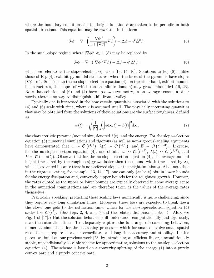
Figure 2: Semi-log plots of the temporal evolution the energy, for a sequence of ε values.The energy decreases like logt until saturation. The dotted lines correspond to the minimumenergy reached by the numerical simulation. The red lines represent the energy plot obtainedby the simulations, while the straight lines are obtained by least squares approximations tothe energy data. Parameters for the fitted lines, which have the form me ln(t) + be, can befound in Tab. 1.

A clear observation of − ln(t) and t1/2 scaling laws can be made, with different coefficientsdependent upon ε.

We have also performed the numerical experiments of the sensitivity in terms of initialrandom data and the numerical resolution. For instance, at ε = 0.02, a simulation with ahigher spatial resolution N = 768 and a smaller time step k = 0.000625 was undertaken, upto t = 400. A numerical comparison between the two resolutions gives almost exact timeevolution history for the energy and standard deviation.

Meanwhile, note that a lower bound for the energy (1) (with a simplified assumptionΩ = (0, L) × (0, L)) has been derived in the earlier article [23]. Based on the followingestimate

F (y) = −1

2ln(1 + |y|2

)≥ −1

2

(α |y|2 − ln(α) + α− 1

), ∀ α ≤ 1 , (52)

13

ε 0.02 0.03 0.04 0.05 0.06 0.07 0.08 0.09 0.10

me -39.62 -38.84 -39.39 -38.21 -38.02 -38.67 -38.66 -39.80 -37.37be -154.24 -125.17 -98.50 -83.66 -74.27 -58.72 -47.06 -37.70 -36.67mr 0.52 0.52 0.51 0.52 0.55 0.55 0.55 0.57 0.56br 0.38 0.38 0.37 0.36 0.34 0.34 0.33 0.32 0.31

Table 1: Fitting parameters for the least squares lines in Figs. 2 and 3. Specifically, theenergy decay lines in Fig. 2 have the form me ln(t) + be, and the roughness lines in Fig. 3have the form brt

mr .

100 101 102 103 104 10510-1

100

101

102

! = 0.09

100 101 102 103 104 10510-1

100

101

102

! = 0.08

100 101 102 103 104 10510-1

100

101

102

! = 0.07

100 101 102 103 104 10510-1

100

101

102

! = 0.06

100 101 102 103 104 10510-1

100

101

102

! = 0.05

100 101 102 103 104 10510-1

100

101

102

! = 0.04

100 101 102 103 104 10510-1

100

101

102

! = 0.03

100 101 102 103 104 10510-1

100

101

102

! = 0.02

100 101 102 103 104 10510-1

100

101

102

! = 0.10

time timetime

roug

hnes

sro

ughn

ess

roug

hnes

s

Figure 3: The log-log plot of the standard deviation (or roughness) of φ, denoted w(t), fora sequence of ε values. For the no slope selection model, w(t) grows like t1/2. The redlines represent the plot obtained by the numerical simulations, while the straight lines areapproximations to the t1/2 growth. In particular, the parameters for the (blue) fitting lines,which have the form brt

mr , can be found in Tab. 1.

14

min

imum

ene

rgy

10!1!700

!650

!600

!550

!500

!450

!400

0.02 0.04

!

Figure 4: (Color online.) Minimum energy versus ε. The star points represent the calculatedminimum energy at saturation. The circles indicate values of the energy lower bound fromEq. (54).

and the elliptic regularity estimate in 2-D

‖∆φ‖2 ≥ 4π2

L2‖∇φ‖2 , ∀ φ ∈ H2

per(Ω) , (53)

with the choice of α = 4ε2π2

L2 , we obtain a lower bound for the energy of the form

E(φ) ≥ L2

2

(ln

(4ε2π2

L2

)− 4ε2π2

L2+ 1

)=: γ . (54)

As can be seen from the results of the numerical simulations, although such a boundis not sharp, the calculated minimum energies for different ε match those predicted by theformula to within 3% accuracy.

Another interesting issue is the saturation time scale and its dependence on the physicalparameter ε. A formal argument shows an intuitive O(ε−2) law for the saturation time scale.

This time scale is also explored in our numerical simulation rersults. For each ε, thecorresponding energy plot (vs time) indicates an approximate −log(t) law, with appropriatecoefficients given by Figure 2. We define the saturation time as the intersection value (fortime) of such an approximate line with the horizontal line with the final actually reachedsteady energy (obtained by the numerical simulation other than formula (54)).

Figure 5 gives the plot of the saturation time vs ε. The star lines represent the valuesobtained by the numerical simulations, while the circle lines give the least square approxi-mation to these numerical data. Moreover, this approximation gives a slope of −2.04, whichis almost a perfect match with the O(ε−2) scaling law.

15

satu

ratio

n tim

e

10!1104

105

106

0.02 0.04

!

Figure 5: Log-log plot of saturation time versus ε. The star points represent the valuesobtained by the numerical simulation, and the line with circles represent the least squaresapproximation to these data. The slope of the fitting line is -2.04.

5 Summary

We have presented an unconditionally stable convergent liner scheme for a model for thinfilm epitaxy without slope selection. The unconditional stability and convergence followsdirectly from our general result on convex splitting approach to models of thin film epitaxialgrowth [23]. The current scheme is fully linear in the sense that a linear symmetric (bi-harmonic type) problem only is solved at each time step. The unconditional stability of thefully discrete scheme under collocation Fourier spectral approximation is also verified. Thenew scheme is then implemented utilizing FFT. Various physical scaling laws of the modelin terms of energy decay, system roughness and saturation time are recovered and verifiednumerically.

The work here also demonstrates a subtlety involved in terms of the (non-unique) convexsplitting method with some of the schemes (like the one that we proposed here) possiblymuch more efficient than others (such as those proposed in our previous work [23]) althoughall of them enjoy unconditional stability.

Acknowledgment

This work was initiated while Xiaoming Wang was visiting Wenbin Chen at Fudan Universityin 2008. The work is supported in part by the National Science Foundation (DMS0606671,DMS1008852, DMS1002618), the Modern Applied Mathematics 111 Project at Fudan Uni-versity, and ...

16

References

[1] Bertozzi, A.L., Esedoglu, S. and Gillette A.; Inpainting of binary images using theCahn-Hiliard equation, IEEE trans. Image Proc., 16 (2007) 285-291.

[2] Cheng, M., and Warren, J.A., An efficient algorithm for solving the phase field crystalmodel, J. Comput. Phys., 227 (2008) 6241-6248.

[3] Du, Q., Nicolaides, R., Numerical analysis of a continuum model of a phase transition,SIAM J. Num. Anal., 28, (1991), pp. 1310-1322.

[4] Ekeland, I. and Temam, R.; Convex analysis and variational problems, SIAM, Philadel-phia, PA, 1999.

[5] Elliott, C.M., The Cahn-Hilliard model for the kinetics of phase separation, in Mathe-matical Models for Phase Change Problems, J.F. Rodrigues, ed., BirkhauserVerlag, Basel, (1989) 35-73.

[6] Ehrlich, G. and Hudda, F.G., Atomic view of surface diffusion: Tungsten on tungsten,J. Chem. Phys., 44, (1966) 1036-1099.

[7] Evans, L.C.; Partial Differential Equations, AMS, Providence, RI, 1998.

[8] Evans, J.W., Thiel, P.A., and Bartelt, M.C.; Morphological evolution during epitaxialthin film growth: Formation of 2D islands and 3D mounds, Surface Science Re-ports 61 (2006) 1128.

[9] Eyre, D.J.; Unconditionally gradient stable time marching the Cahn-Hilliard equation,in Computational and Mathematical Models of Microstructural Evolu-tion, J. W. Bullard, R. Kalia, M. Stoneham, and L.Q. Chen, eds., Materials ResearchSociety, Warrendale, PA, 53 (1998) 1686-1712.

[10] Giaquinta, M.; Multiple Integrals in the Calculus of Variations and Nonlinear EllipticSystems, Princeton University Press, Princeton, NJ, 1983.

[11] Hu, Z., Wise, S.M., Wang, C. and Lowengrub, J.S.; Stable and efficient finite-differencenonlinear-multigrid schemes for the Phase Field Crystal equation, J. Comput. Phys.,228 (2009) 5323-5339.

[12] Johnson, M.D., Orme, C., Hunt, A.W., Graff, D., Sudijono, J., Sander, L.M., and Orr,B.G.; Stable and unstable growth in molecular beam epitaxy, Phys. Rev. Lett., 72(1994) 116119.

[13] Kohn, R.V.; Energy-driven pattern formation, in Proceedings of the Interna-tional Congress of Mathematicians, M. Sanz-Sole, J. Soria, J.L. Varona, andJ. Verdera, eds., European Mathematical Society Publishing House, Madrid, 1 (2006)359-383.

[14] Kohn, R.V. and Yan, X.; Upper bound on the coarsening rate for an epitaxial growthmodel, Comm. Pure Appl. Math., 56 (2003) 1549-1564.

17

[15] Kohn, R.V. and Yan, X.; Coarsening rates for models of multicomponent phase separa-tion, Interfaces and Free Boundaries, 6 (2004) 135-149.

[16] Li, B. and Liu, J.-G.; Thin film epitaxy with or without slope selection, Euro. J. Appl.Math., 14 (2003) 713-743.

[17] Li, B. and Liu, J.-G.; Epitaxial growth without slope selection: energetics, coarsening,and dynamic scaling, J. Nonlinear Sci., 14 (2004) 429-451.

[18] Moldovan, D. and Golubovic L.; Interfacial coarsening dynamics in epitaxial growthwith slope selection, Phys. Rev. E, 61 (2000) 6190-6214.

[19] Schwoebel, R.L.; Step motion on crystal surfaces: II, J. Appl. Phys., 40 (1969) 614-618.

[20] Temam, R.; Navier-stokes equations and nonlinear functional analysis, SIAM, Philadel-phia, PA, 1995.

[21] Vollmayr-Lee, B. P. and Rutenberg, A.D.; Fast and accurate coarsening simulation withan unconditionally stable time step, Phys. Rev. E, 68 (2003) 066703.

[22] Wise, S.M., Wang, C. and Lowengrub, J.; An energy stable and convergent finite-difference scheme for the Phase Field Crystal equation, SIAM J. Numer. Anal.,47, (2009) 2269-2288.

[23] Wang, C., Wang, X. and Wise, S.M.; Unconditionally stable schemes for equations ofthin film epitaxy, Discrete and Continuous Dynamical Systems-Series A, 28,(2010) 405-423.

[24] Xu, C and Tang, T.; Stability analysis of large time-stepping methods for epitaxial growthmodels, SIAM J. Numer. Anal., 44, (2006) 1759-1779.

18