a linear time-invariant consensus dynamics with homogeneous delays: analytical study and synthesis...

Copyright © by SIAM. Unauthorized reproduction of this article is prohibited.

SIAM J. CONTROL OPTIM. c© 2013 Society for Industrial and Applied MathematicsVol. 51, No. 5, pp. 3971–3992

A LINEAR TIME-INVARIANT CONSENSUS DYNAMICS WITHHOMOGENEOUS DELAYS: ANALYTICAL STUDY AND

SYNTHESIS OF RIGHTMOST EIGENVALUES∗

WEI QIAO† AND RIFAT SIPAHI‡

Abstract. This paper investigates the rightmost eigenvalue behavior of a class of single-delaylarge-scale consensus dynamics where information shared among the agents is delayed. We presentan analytical approach that links stabilizing effects of delays to the finite number of graph Laplacianeigenvalues associated with the network and to the coupling strengths between the agents. In par-ticular, we extend our previously developed concept called Responsible Eigenvalue (RE), which isconcerned with the delay margin of the dynamics, to the analysis of how the infinitely many eigen-values of the dynamics are configured on the complex plane. We show that, under certain conditionsof the graph Laplacian eigenvalues, the rightmost eigenvalue can be placed farther from the imagi-nary axis of the complex plane for larger delays. This information leads to rules by which couplingstrengths of the agents can be designed to reduce the settling time of the system, rendering theconsensus dynamics delay tolerant. Numerical examples are provided to demonstrate the stabilizingeffects of delays, including uncertainties in delays, and simulation results are presented to show theimprovements in transient response of the consensus dynamics.

Key words. LTI consensus system, heterogeneous agents, homogeneous delays, rightmost roots

AMS subject classifications. 93A15, 93B52, 93C15, 34A35

DOI. 10.1137/110832574

1. Introduction. Many dynamical systems found in economics, biology, physics,and control theory can be modeled with delay-differential equations [13, 25, 30, 54, 60].In these fields, stability analysis of coupled agents with time delay has become an at-tractive topic within the past decade [2, 10, 18, 20, 21, 34, 37, 48, 49, 50]. In such sys-tems, network connectivity ensures the coupling of the agents, but the communicationdelay between the connected agents affects the coupled-system functionality. That is,topology and time delay together play an important role in the stability of the entiresystem. Analyzing stability at the interplay between topology and time delay is, how-ever, complicated since the information one agent receives from another at an instantdepends on both the network connectivity and delay τ [43, 44, 45, 46, 48, 49, 57, 58].Applications in this context are found in consensus dynamics, vehicular traffic flownetworks, coupled oscillators, supply chains, synchronization problems, and neuralnetworks [16, 17, 24, 41, 42, 47, 50, 59].

For coupled time-delay systems, the existing literature is mainly concernedwith designing stabilizing controllers, analyzing stability with respect to the delayparameter, finding conditions for stability, and detecting the delay margin of thesystem at hand, where delay margin τ∗ is known as the maximum amount of thedelay less than which a system remains stable [6, 8, 27, 32, 38]. Many results existalong these lines, including data networks [1], multiagent consensus and rendezvous

∗Received by the editors May 2, 2011; accepted for publication (in revised form) July 5, 2013;published electronically October 16, 2013. This work was supported in part by National ScienceFoundation award ECCS 0901442.

http://www.siam.org/journals/sicon/51-5/83257.html†Department of Mechanical and Industrial Engineering, Northeastern University, Boston, MA

02115 ([email protected]).‡Corresponding author. Department of Mechanical and Industrial Engineering, Northeastern

University, Boston, MA 02115 ([email protected]).

3971

Dow

nloa

ded

11/2

0/13

to 1

34.9

9.12

8.41

. Red

istr

ibut

ion

subj

ect t

o SI

AM

lice

nse

or c

opyr

ight

; see

http

://w

ww

.sia

m.o

rg/jo

urna

ls/o

jsa.

php


3972 WEI QIAO AND RIFAT SIPAHI

problems [11, 37], teleoperation [19], manufacturing, stabilization, observer design[54], traffic flow [25, 30, 40, 50], complexity issues [61], and stability analysis tech-niques [14, 15, 22, 23, 49, 51, 52, 55, 56, 60].

This paper focuses on a broadly studied linear time-invariant (LTI) consensus dy-namics [11, 18, 20, 36, 37, 47] with a corresponding graph Laplacian L, and where asingle constant delay τ exists in all interagent communication channels. For thisdynamics, our previously developed concept, called Responsible Eigenvalue (RE)[44, 45, 46, 57, 58], reveals the delay margin τ∗ in connection with the finite numberof eigenvalues of L. This result in one sense establishes a direct link between τ∗ andgraph Laplacian eigenvalues despite the fact that stability analysis is concerned withinfinitely many eigenvalues. We take this result one step further here by studyinganalytically the behavior of all these infinitely many eigenvalues on the complex planewith respect to the delay parameter and the eigenvalues of L. Specifically, we showthat settling time of the consensus dynamics can be reduced as approximated by therightmost eigenvalues for some τ �= 0 if and only if all the eigenvalues of the negativegraph Laplacian (−L) are stable and all have in magnitude larger real parts thanimaginary parts. Although stabilizing effects of delays are known [33, 39, 60], this an-alytical result is practical, as it ties stability characteristics of the consensus dynamicswith the graph Laplacian eigenvalues. These conditions show that some particulartopologies and graph Laplacian eigenvalue configurations affect the behavior of theinfinitely many eigenvalues of the dynamics at hand in a way that favors the dynamicsto become more tolerant to delays. Although this result is based on a single-delaymodel, it demonstrates opportunities for designing the graphs and topologies of time-delay systems so that delays, even if they are inevitable, can actually be used toimprove dynamic behavior as measured by rightmost eigenvalues.

The paper is organized as follows. In section 2, an example is given for motivation,and in section 3, some definitions related to graphs, stability, and delay margin arecovered, and the consensus dynamics is presented. The main results follow in section 4,and the numerical examples, including robustness analysis against delay uncertainties,are presented in section 5. Conclusions and future research directions end the paperin section 6.

In this paper, C+ and C− denote, respectively, the set of complex numbers withpositive and negative real parts. The relative complement of a set B in another setA is denoted by {A\B}. We use s ∈ C for the Laplace variable on the complexplane, �(s) for the real and �(s) for the imaginary parts of s, and R+ for positiveand R− for negative real numbers. To distinguish Laplace transformation and graphLaplacians, we cite, respectively, [35] and [7]. τ ≥ 0 is the delay. Eigenvalues ofa square matrix A ∈ Rn×n are denoted by λ1(A), . . . , λk(A), . . . , λn(A). In themultivariable function f (a1; a2, . . . , ap), a1 denotes the variable of the function, whilea2, . . . , ap are the parameters, and the roots of f (a1; a2, . . . , ap) are associated witha1 = a1(a2, . . . , ap). We omit the arguments when no confusion occurs.

2. Motivation. In this section, we present an example of how the rightmosteigenvalues can move farther to the left of the imaginary axis of the complex plane asthe delay parameter increases. This example motivates the remainder of the paper.

In Figure 2.1, rightmost eigenvalue trajectories are depicted on the complex plane,using TRACE-DDE [5], as time delay is increased from zero, in a representative LTIsystem. In this example, we see that the rightmost eigenvalues move away fromthe imaginary axis as the delay increases and then turn around to approach theimaginary axis as the delay becomes much larger. As we show and prove in section 4

Dow

nloa

ded

11/2

0/13

to 1

34.9

9.12

8.41

. Red

istr

ibut

ion

subj

ect t

o SI

AM

lice

nse

or c

opyr

ight

; see

http

://w

ww

.sia

m.o

rg/jo

urna

ls/o

jsa.

php


ANALYSIS AND SYNTHESIS OF RIGHTMOST EIGENVALUES 3973

Fig. 2.1. Rightmost eigenvalue trajectories on the complex plane for a representative LTIsystem. Green arrows show the direction of increasing time delay. Root locations are computed byTRACE-DDE [5].

for the type of LTI systems studied here, when the graph Laplacian eigenvalues satisfycertain conditions, the rightmost eigenvalues of the system indeed move away from theimaginary axis for certain delays. These conditions can be useful, as they can lead tothe rules by which the system at hand can be designed to be delay tolerant for nonzerodelays, by reducing its settling time approximated by the rightmost eigenvalues, aswas also shown in several studies in the literature; see, e.g., [29, 31].

3. Preliminaries.

3.1. Basic algebraic graph theory. An nth order digraph (directed graph) Gis an ordered double [V(G), E(G)] consisting of a set of vertices V(G) = {ν1, ν2, . . . , νn}and a set of edges E(G) with edges denoted by eik = (νi, νk) ∈ E(G). Each vertexof a graph G is indicated by a point, and each edge is indicated by a directed linefrom one vertex to another. We extend this definition by considering that an agentwith a dynamics resides at each vertex (node) and couples with the other dynamicsat the other vertices through the edges. The coupling strength, aik, on the edge eikdefines how strongly the dynamics at νi couples with the one at νk. Furthermore,the coupling facilitates information sharing among the agents, but the informationarriving at the agents at time t is the information released from other agents at timet − τ . Moreover, the adjacency matrix D = [dik] of a weighted digraph is defined asdii = 0, and dik > 0 if (νi, νk) ∈ E(G), where i �= k. The graph Laplacian of thisweighted digraph is defined as L = [lik], where lii =

∑nk=1,k �=i dik and lik = −dik for

i �= k [28].

3.2. Agent dynamics and system description. We start with a broadlystudied LTI consensus dynamics, which can also be found in similar forms in [26, 34,44, 45, 46, 50, 53, 57],

xi(t) = ui(t),

ui(t) =

n∑k=1,k �=i

aik [xk(t− τ) − xi(t− τ)] , i = 1, . . . , n,(3.1)

where xi(t) is the state of the ith agent, constant coupling strength is nonnegative,aik ≥ 0, and agent i receives the state information of agent k whenever aik �= 0. In(3.1), τ is the nonnegative constant delay, which influences the controller ui(t) appliedon agent i. Equation (3.1) can also be seen as a network of integrator dynamics

Dow

nloa

ded

11/2

0/13

to 1

34.9

9.12

8.41

. Red

istr

ibut

ion

subj

ect t

o SI

AM

lice

nse

or c

opyr

ight

; see

http

://w

ww

.sia

m.o

rg/jo

urna

ls/o

jsa.

php



[11, 33, 37, 47] that attempt to synchronize their states with respect to each otherusing the controller ui(t).

We can express (3.1) in vector form as

(3.2) x(t) = Ax(t− τ),

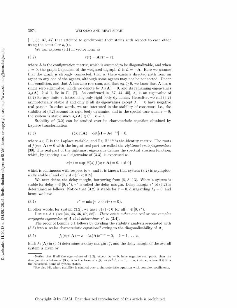
where A is the configuration matrix, which is assumed to be diagonalizable, and whenτ = 0, the graph Laplacian of the weighted digraph L is L = −A. Here we assumethat the graph is strongly connected; that is, there exists a directed path from anagent to any one of the agents, although some agents may not be connected. Underthis condition, and that A has zero row sum, and that aik ≥ 0, we know that A has asingle zero eigenvalue, which we denote by λ1(A) = 0, and its remaining eigenvaluesλk(A), k �= 1, lie in C− [7]. As confirmed in [57, 44, 45], λ1 is an eigenvalue of(3.2) for any finite τ , introducing only rigid body dynamics. Hereafter, we call (3.2)asymptotically stable if and only if all its eigenvalues except λ1 = 0 have negativereal parts.1 In other words, we are interested in the stability of consensus, i.e., thestability of (3.2) around its rigid body dynamics, and in the special case when τ = 0;the system is stable since λk(A) ∈ C−, k �= 1.

Stability of (3.2) can be studied over its characteristic equation obtained byLaplace transformation,

(3.3) f (s; τ,A) = det[sI−Ae−τs] = 0,

where s ∈ C is the Laplace variable, and I ∈ Rn×n is the identity matrix. The rootsof f (s; τ,A) = 0 with the largest real part are called the rightmost roots/eigenvalues[30]. The real part of the rightmost eigenvalue defines the spectral abscissa function,which, by ignoring s = 0 eigenvalue of (3.3), is expressed as

σ(τ) = sup{�(s)|f (s; τ,A) = 0, s �= 0},which is continuous with respect to τ , and it is known that system (3.2) is asymptot-ically stable if and only if σ(τ) < 0 [9].

We next define the delay margin, borrowing from [6, 8, 13]. When a system isstable for delay τ ∈ [0, τ∗), τ∗ is called the delay margin. Delay margin τ∗ of (3.2) isdetermined as follows. Notice that (3.2) is stable for τ = 0, disregarding λ1 = 0, andhence we have

(3.4) τ∗ = min{τ > 0|σ(τ) = 0}.In other words, for system (3.2), we have σ(τ) < 0 for all τ ∈ [0, τ∗).

Lemma 3.1 (see [44, 45, 46, 57, 58]). There exists either one real or one complexconjugate eigenvalue of A that determines τ∗ in (3.4).

The proof of Lemma 3.1 follows by dividing the stability analysis associated with(3.3) into n scalar characteristic equations2 owing to the diagonalizability of A,

(3.5) fk(s; τ,A) = s− λk(A)e−τs = 0, k = 1, . . . , n.

Each λk(A) in (3.5) determines a delay margin τ∗k , and the delay margin of the overallsystem is given by

1Notice that if all the eigenvalues of (3.2), except λ1 = 0, have negative real parts, then thesteady-state solution of (3.2) is in the form of xi(t) → βeλ1t, i = 1, . . . , n, t → ∞, where β ∈ R isthe consensus point of system states.

2See also [4], where stability is studied over a characteristic equation with complex coefficients.

Dow

nloa

ded

11/2

0/13

to 1

34.9

9.12

8.41

. Red

istr

ibut

ion

subj

ect t

o SI

AM

lice

nse

or c

opyr

ight

; see

http

://w

ww

.sia

m.o

rg/jo

urna

ls/o

jsa.

php



(3.6) τ∗ = mink=2,...,n

(τ∗k ).

In our recent work [44, 45, 46, 57], the eigenvalue λk that minimizes τ∗k in (3.6) iscalled the Responsible Eigenvalue (RE). The RE is directly linked to τ∗, which is usefulfor analyzing τ∗ as a parameter of λk. However, the RE concept does not explain howthe infinitely many eigenvalues of (3.2) move on the complex plane. The knowledgeof how these eigenvalues move on C could provide richer information, especially fromthe viewpoints of settling time and damping characteristics of (3.2) as approximatedby the rightmost eigenvalues. This is what we focus on in section 4.

4. Main results. Under the assumptions mentioned in the previous section, weknow that system (3.2) is asymptotically stable around its rigid body dynamics, forall τ ∈ [0, τ∗), where τ∗ is defined as in (3.6). To address a more general result, theproblem is extended here to the study of eigenvalue behavior of (3.2) on C as thedelay parameter τ varies from zero to τ∗.

When τ is perturbed from zero to 0+, following from [3, 9], one knows that oneof the eigenvalues of (3.2) remains on the origin,3 denoted here by s1 = λ1 = 0; n− 1number of them, sk, emanate from λk(A), k = 2 . . . n; and the remaining infinitelymany of them, sk,r arise at −∞ on C . The trajectories Lk and Lk,r formed on C,respectively, by sk(τ) and sk,r(τ), k = 2, . . . , n, r = 1 . . . ,∞, create a complicatedoutlook as τ : 0 → τ∗, which is difficult to analyze. To systematically approach this,we first focus on studying the problem for a fixed k, k �= 1.

We start by substituting4 s = σk+jωk into (3.5), where σk < 0 as per the problemat hand, and we let λk(A) = ρke

jθk , where ρk > 0 and θk ∈ (π/2, 3π/2), which yields

(4.1) fk(σk + jωk; τ,A) := σk + jωk − ρkejθke−τ(σk+jωk) = 0,

which, with some manipulations, becomes

(4.2)

{σk(ωk) = ωk cot(θk − τωk) : σ − curve,

ωk(σk) = ±√ρ2ke

−2τσk − σ2k : ω − curve.

Notice that, given λk and τ , by sweeping ωk in the first equation and σk inthe second equation of (4.2), we can obtain sufficiently many points with which thesimultaneous solutions of (4.2), and consequently the rightmost eigenvalue, can bereliably approximated. However, this is not the main objective here, as efficientnumerical rightmost-root solvers exist in the literature [5, 62, 63, 64, 65]. We arerather interested in analytically studying how the real part σk of the eigenvalueschanges with respect to the delay parameter τ .

Definition 4.1. Let αk(τ) :=∣∣∣ωk(τ)σk(τ)

∣∣∣ > 0, where τ ≥ 0, and s = σk + jωk

satisfies (4.1).Lemma 4.2. When (4.1) holds for a root s = σk + jωk ∈ C− with ωk > 0, the

following conditions are simultaneously satisfied:(a) dωk

dτ

∣∣τ=0

> 0;

(b) dωk

dτ

∣∣τ=τk

= 0 with τk = − 2σk(α2

k+1);

(c) d2ωk

dτ2

∣∣∣τ=τk

< 0.

3s = 0 is a solution of (3.5) for any finite τ ≥ 0 since λ1(A) = 0.4Notice here that s(τ) = {⋃n

k=2 sk(τ)}⋃{⋃n

k=2

⋃∞r=1 sk,r(τ)}

⋃{0}, τ ≥ 0.

Dow

nloa

ded

11/2

0/13

to 1

34.9

9.12

8.41

. Red

istr

ibut

ion

subj

ect t

o SI

AM

lice

nse

or c

opyr

ight

; see

http

://w

ww

.sia

m.o

rg/jo

urna

ls/o

jsa.

php



Proof. The proof is divided into three parts.(a) The following derivative is calculated using (4.1):

(4.3)dωk

dτ= −�

[∂fk/∂τ

∂fk/∂ωk

]:=

N(τ)

D(τ)= −ωk((σ

2k + ω2

k)τ + 2σk)

(τωk)2 + (1 + τσk)2.

From (4.3), it is easy to see that sk → λk(A), k �= 1, as τ → 0+, and thus σk =�(λk(A)) < 0.

(b) Setting (4.3) to zero and solving for τ gives τk = − 2σk(α2

k+1), which always

exists since σk < 0.(c) From (4.3), we have

(4.4)d2ωk

dτ2=D(τ)∂N(τ)/∂τ −N(τ)∂D(τ)/∂τ

D2(τ).

Since N(τk) = 0 and D(τ) > 0 for any τ ≥ 0, from (4.4), we have

d2ωk

dτ2

∣∣∣∣τ=τk

=1

D(τ)

∂N(τ)

∂τ

∣∣∣∣τ=τk

= − ωk(σ2k + ω2

k)

(τkωk)2 + (1 + τkσk)2< 0,

from which we conclude that condition (c) holds for ωk > 0, indicating that ωk > 0makes a maximum in C− at τ = τk.

Lemma 4.3. The following conditions hold for a root s = σk+jωk ∈ C− satisfying(4.1):

(a) dσk

dτ

∣∣τ=0

< 0 if and only if αk(0) < 1;

(b) dσk

dτ

∣∣τ=τ∗∗

k

= 0 whenever τ = τ∗∗k :=α2

k−1

σk(α2k+1)

> 0;

(c) d2σk

dτ2

∣∣∣τ=τ∗∗

k

> 0 if condition (b) holds;

(d) τk > τ∗∗k > 0.Proof. The proof is divided into four parts.

(a) Using fk = 0 in (4.1) to simplify the expression dσk

dτ = −�[ ∂fk/∂τ∂fk/∂σk

] found

again from (4.1), one obtains

(4.5)dσkdτ

= −σ2k(1 + τσk − α2

k(1− σkτ))

(τωk)2 + (1 + τσk)2,

from which condition (a) follows. Since this condition is for τ → 0, it holds for one ofthe eigenvalues sk → λk(A), k = 2, . . . , n.

(b) Set (4.5) to zero and solve for τ > 0, which leads to condition (b). This alsoimplies that αk(τ

∗∗k ) < 1 holds when condition (b) holds.

(c) Note that

(4.6)d2σkdτ2

∣∣∣∣τ=τ∗∗

k

= − σk(1 + α2k)

(τ∗∗k ωk)2 + (1 + τ∗∗k σk)2> 0,

so long as τ∗∗k > 0 exists. This condition, together with condition (b), indicates thatthere exists an eigenvalue s(τ), real part σk of which makes a minimum at τ = τ∗∗k .

(d) By comparing τk and τ∗∗k , it is easy to see that condition (d) holds, since σk < 0and αk(τ) < 1 are automatically satisfied when these delay values are positive. Underthis setting, one has that, for an eigenvalue s(τ), σk reaches its minimum at a smallerdelay τ = τ∗∗k than ωk > 0 reaching its maximum at delay τ = τk.

Dow

nloa

ded

11/2

0/13

to 1

34.9

9.12

8.41

. Red

istr

ibut

ion

subj

ect t

o SI

AM

lice

nse

or c

opyr

ight

; see

http

://w

ww

.sia

m.o

rg/jo

urna

ls/o

jsa.

php



Fig. 4.1. Trajectories (representative drawing) of the eigenvalues sk and sk,1, . . . , sk,∞ as thedelay τ increases from zero, k �= 1. The straight line shows the condition αk(0) = 1 on the thirdquadrant of C, which is |�(λk(A))| = |�(λk(A))|.

In Figure 4.1, a pictorial example5 is given regarding how the eigenvalues mightmove on the complex plane as delay τ changes, where the bold straight line showsthe condition αk(0) = 1 on the third quadrant of C, and the dashed curves show theeigenvalue locations as delay τ increases. When τ = 0, the eigenvalue sk(τ = 0) =λk(A) is below the line equation |�(λk(A))| = |�(λk(A))|, satisfying the requirementαk(0) < 1 in Lemma 4.3. Hence, as τ changes from 0 to 0+, the eigenvalue sk, whichdeparts from λk at τ = 0, moves to the left and away from the real axis. However, it isinconclusive at this point whether or not the remaining properties in Lemma 4.2–4.3hold for sk as well, and hence Figure 4.1 should be considered with this precaution.6

We know, however, that at least one eigenvalue satisfies these properties. The realpart σk reaches its smallest value when τ = τ∗∗k at the point P1 marked with a star.For τ = τk, which is greater than τ∗∗k as per Lemma 4.3, the imaginary part ωk > 0reaches its maximum at point Q1.

We note that points P1 and Q1 on C are different for each counter k. Also, asτ increases, infinitely many eigenvalues sk,1, . . . , sk,∞ merge along the loci Lk,r. Inthe presence of all these eigenvalues, it is not easy to identify which eigenvalue(s) areresponsible for generating the rightmost eigenvalue(s) for different τ values, and itis not yet possible to claim that what is proven in Lemma 4.2–4.3 is valid for therightmost eigenvalues. These issues are addressed in what follows.

In order to tackle the aforementioned problems, one could study the behaviorof the roots of (4.1), which can be analyzed by investigating the intersection pointsbetween the two curves defined in (4.2), as we demonstrate in what follows. Theω-curve is a semicircle C1 with radius ρk when τ = 0 (see Figure 4.2), where thedashed part is omitted since σk < 0. When τ increases from 0 to 0+, anothercurve C2 generated at σk → −∞ emanates, while the semicircle C1 distorts, movingtoward C2.

5Notice that these trajectories do not necessarily correspond to a realistic mathematical model,but they are provided to explain the subsequent discussions.

6In the sequel, proofs are presented to show that indeed the eigenvalue movement is qualitativelyas depicted in Figure 4.1.

Dow

nloa

ded

11/2

0/13

to 1

34.9

9.12

8.41

. Red

istr

ibut

ion

subj

ect t

o SI

AM

lice

nse

or c

opyr

ight

; see

http

://w

ww

.sia

m.o

rg/jo

urna

ls/o

jsa.

php



Fig. 4.2. Representative ω-curve. Arrows show the direction of increasing τ , the dashed partof the circle is neglected since the ω-curve is studied under the condition σk < 0, and, in this plot,we have ρk = 15.

When the two separate segments C1 and C2 of the ω-curve merge into each other,singularity points arise for critical delay values τ

′k. Singularities can be studied by

first rewriting the ω-curve in (4.2) as

F(σk, ωk) := ω2k + σ2

k − ρ2ke−2τkσk = 0.

The singular points (σ′k, ω

′k) can be computed [12] from the simultaneous solutions of

F = 0, ∂F/∂σk = 0, ∂F/∂ωk = 0.

We find that this happens only on σk axis at σ′k = −ρke with ω

′k = 0, and only for

one delay value,

(4.7) τ′k = − 1

σ′k

=1

ρke,

which is a function of only ρk = |λk(A)|, where e is the base of the natural logarithm.In Figure 4.3, the ω-curve is depicted for τ = τ

′k and τ = τ

′k + ε, |ε| 1.

The σ-curve is a line when τ = 0 and becomes a transcendental function forτ > 0; see Figure 4.4. The frequency τωk of the cotangent in the σ-curve increasesas τ increases. The curve intersects with the ω-axis at ω1 = 0 and whenever cot(θk −τωk) = 0, which indicates that the rest of the intersection points are at ωl =

θk−π2 ∓πl

τ ,l = 2, . . . .

Fig. 4.3. Representative ω-curve for τ = τ′k and τ = τ

′k + ε, |ε| 1, where ρk = 15.

Dow

nloa

ded

11/2

0/13

to 1

34.9

9.12

8.41

. Red

istr

ibut

ion

subj

ect t

o SI

AM

lice

nse

or c

opyr

ight

; see

http

://w

ww

.sia

m.o

rg/jo

urna

ls/o

jsa.

php



Fig. 4.4. σ-curve in (4.2) for θk = 13π18

.

Definition 4.4 (k is fixed, k �= 1). Let σk(τ) be the real part of the rightmost ofthe infinitely many eigenvalues on the loci Lk,1, . . . , Lk,∞, and let σ∗

k be the real partof the single eigenvalue on the locus Lk.

We next study the singularity points of the σ-curve in (4.2) by first rewritingit as

G(σk, ωk) = σk − ωk cot(θk − τkωk) = 0.

One finds that the derivative ∂G/∂σk = 1 is nonzero, indicating that the σ-curve is anonsingular curve [12] and thus cannot fold onto itself. When τ → 0+, the σ-curveintersects with the C2 segment of the ω-curve at σk → −∞. However, for τ → 0+, wehave ωl → ±∞, l = 2, . . ., and therefore the σ-curve intersects with the C1 segment ofthe ω-curve only in finite σk domain when τ → 0+. Hence, as τ increases from zeroto 0+, the roots with real part at −∞ on the loci Lk,1, . . . , Lk,∞ are found from theintersection points between C2 and the σ-curve, only at σk → −∞. Therefore for afixed k, k �= 1, all σk at these intersection points have smaller negative values thanthe σk values on C1; that is, |σ∗

k(τ)| < |σk(τ)| holds for τ : 0 → 0+, and hence theeigenvalue sk,r is located to the left of the eigenvalue sk, r = 1, . . . ,∞.

Lemma 4.5 (λk(A) ∈ {C−\R−} case). The condition |σ∗k(τ)| < |σk(τ)| holds

for 0 ≤ τ < τ∗k .Proof. Let sk(τ) = σ∗

k + jΩk and sk,r(τ) = σk,r + jΩk,r be two roots of (4.1)on, respectively, the locus Lk and Lk,r. The proof can be established by showingthat the root sk,r always remains to the left of the sk root. Since sk,r(τ = 0+) ison the left of sk(τ = 0+) as discussed above, it suffices to show in the following that�(sk) �= �(sk,r) holds for all delay values less than the delay margin τ∗k :

(a) There does not exist a τ value such that σ∗k = σk,r and Ωk = Ωk,r simulta-

neously hold, since we have shown above that the σ-curve is a nonsingularcurve, and the only singular point of the ω-curve exists on the σk axis, whichcannot be a feasible solution since λk ∈ {C−\R−}.

(b) There does not exist a τ value such that σ∗k = σk,r and Ωk �= Ωk,r hold for

a given λk ∈ {C−\R−}. This property can be proved by substituting thereal and imaginary parts of sk(τ) and sk,r(τ) into the ω-curve in (4.2), whichleads to Ωk = −Ωk,r. For Ωk = −Ωk,r, the σ-curve in (4.2) is then solved,which gives only one feasible solution,

(4.8) θk = π,

Dow

nloa

ded

11/2

0/13

to 1

34.9

9.12

8.41

. Red

istr

ibut

ion

subj

ect t

o SI

AM

lice

nse

or c

opyr

ight

; see

http

://w

ww

.sia

m.o

rg/jo

urna

ls/o

jsa.

php



since θk ∈ (π2 ,3π2 ) must hold. However, θk = π is ruled out since θk �= π when

λk ∈ {C−\R−}.Lemma 4.6 (λk(A) ∈ R− case). The following conditions hold:

(i) |σ∗k(τ)| < |σk(τ)| for 0 ≤ τ < τ

′k;

(ii) σ∗k(τ) = σk(τ) for τ

′k ≤ τ < τ∗k .

Proof. When λk ∈ R−, the σ-curve vanishes since ωk = 0, not requiring simul-taneous solutions of the equations in (4.2). Also, at τ = 0, the ω-curve reduces to apoint at σk = −ρk, which indicates αk = 0. Consequently, using this information, thedelay value at the turning point simplifies as τ∗∗k = − 1

σ∗k, where σ∗

k = −ρke, whichis the exact same expression as τ

′k in (4.7). Thus, for 0 ≤ τ < τ

′k, segments C1 and

C2 of the ω-curve are disjoint (see also Figure 4.2–4.3), and hence one concludes that|σ∗

k(τ)| < |σk(τ)| holds, proving (i). By increasing τ from zero, the eigenvalue thatlies on the real axis moves to the left and merges, on the real axis, into its counter-part emanating from −∞ when the condition τ = τ

′k = τ∗∗k holds. This is exactly

where the singularity occurs when the C1 and C2 segments of the σ-curve in Figure4.2 touch each other on the σk axis for τ = τ

′k. When the delay is infinitesimally

increased to τ = τ′k + ε, 0 < ε 1 (see also Figure 4.3), the two eigenvalues become

complex conjugate, as shown in (4.8) for the condition θk = π, i.e., λk ∈ R−. Sincethere exists no other singularity points on the real axis on the ω-curve, we know thatthese eigenvalues remain in complex conjugate form, which ultimately indicates thatσ∗k(τ) = σk(τ) for all τ

′k ≤ τ < τ∗k proving (ii).

Corollary 4.7. The following conditions simultaneously hold for a fixedk, k �= 1:

(a) dσk

dτ

∣∣τ=0

< 0;

(b) dσk

dτ

∣∣τ=τ∗∗

k

= 0;

(c) d2σk

dτ2

∣∣∣τ=τ∗∗

k

> 0;

(d) τk > τ∗∗kif and only if αk(0) =

∣∣∣ωk(0)σk(0)

∣∣∣ = ∣∣∣�(λk(A))�(λk(A))

∣∣∣ < 1.

Proof. From Lemmas 4.5 and 4.6, we know that the eigenvalue sk on the locus Lk

moves farther from the imaginary axis as the rightmost eigenvalue for τ ∈ [0, τ∗∗k ), andhence we focus on this particular eigenvalue in the rest of the proof. Recall that thisis based on conditions (a)–(c) as τ → 0+. That is, condition (a) is necessary, which issatisfied if and only if αk(0) < 1. When αk(0) < 1, the locus can turn either clockwiseor counter clockwise as τ increases from zero to τ∗∗k . As per Lemma 4.2, however,we know that positive ωk increases when τ increases from zero to τ∗∗k (condition (d)of Lemma 4.3). Hence, the only possibility is that the locus makes a clockwise turnwhile σk decreases as per (a). On the contrary, if αk(0) > 1, then condition (a) doesnot hold, but we have dσk

dτ |τ=0 > 0, and in this case, for σk to make a minimum asper only conditions (b)–(c), it is necessary that the continuous locus Lk makes a localmaximum for some τ = τo < τ∗∗k and makes a global minimum at τ = τ∗∗k . For a local

maximum to exist, it is necessary and sufficient that dσk

dτ in (4.5) is zero and d2σk

dτ2 in(4.6) is negative for τ = τo. Even if the former could hold for some τ = τo, the latteris always positive, which contradicts the assumption αk(0) > 1.

In light of Lemma 4.5, Lemma 4.6, and Corollary 4.7, one can now concludethat the eigenvalue s = σk + jωk that exhibits the properties in Lemmas 4.2 and 4.3is actually one of the sk eigenvalues, k fixed, k �= 1, which reinforces the pictorialexplanation in Figure 4.1.

Dow

nloa

ded

11/2

0/13

to 1

34.9

9.12

8.41

. Red

istr

ibut

ion

subj

ect t

o SI

AM

lice

nse

or c

opyr

ight

; see

http

://w

ww

.sia

m.o

rg/jo

urna

ls/o

jsa.

php



To summarize the above developments, we state that, for a fixed k, k �= 1,(i) each eigenvalue sk moves farther from the imaginary axis for delays in the

range of [0, τ∗∗k ) as long as the eigenvalues of the negative graph Laplacian−L satisfy

|�(λk(A))| > |�(λk(A))| and �(λk(A)) < 0,

where τ∗∗k is the delay value for which sk is the farthest from the imaginaryaxis.

(ii) the eigenvalue sk dictates the rightmost eigenvalue for τ ∈ [0, τ∗k ), not theeigenvalues sk,r arriving from −∞, where τ∗k is the delay margin associatedwith λk(A).

The information in (i)–(ii) is important for two reasons. First, it reveals that un-der certain conditions, the control system is tolerant to delay, indicated by rightmosteigenvalues moving farther from the imaginary axis. Second, it correlates the eigen-value behaviors on the complex plane as well as the rightmost eigenvalues, with λk(A)of the negative graph Laplacian −L = A, allowing the design of the finite number ofeigenvalues of A in order to render specific dynamic behavior from the infinitely manyeigenvalues of the consensus system. In a case study in the following section, we usethis idea to design the graph Laplacian eigenvalues by tuning the agent couplings sothat the rightmost eigenvalues move farther from the imaginary axis for some nonzerodelay.

Now that the rightmost eigenvalue identification is established, we study the iso-τ∗∗k contours that arise from the particular locations of the turning points P1 of therightmost eigenvalues sk, k �= 1, defined in Figure 4.1. These contours, which are

depicted in Figure 4.5, are calculated via the expression τ∗∗k =α2

k−1

σk(α2k+1)

and under

the condition |ωk| < |σk| as per Corollary 4.7, using the mesh command in MATLAB.The points on a contour represent the turning points (similar to P1 in Figure 4.1) ofan eigenvalue sk, depicting how far the turning point can be from the imaginary axisfor the τ = τ∗∗k contour value. We call this contour map “turning point contour map”(TPCM) and elaborate further on it with some lemmas and a corollary.

Lemma 4.8. An eigenvalue s on TPCM at the turning point s = p+ qj with thecontour value τ∗∗k on TPCM is created by a unique λk(A), k �= 1.

Fig. 4.5. Iso-τ∗∗k contours, with contour locations indicating the turning points of the rightmosteigenvalues sk. τ

∗∗k monotonically decreases as σk < 0 decreases for a given αk = tan(ψk).

Dow

nloa

ded

11/2

0/13

to 1

34.9

9.12

8.41

. Red

istr

ibut

ion

subj

ect t

o SI

AM

lice

nse

or c

opyr

ight

; see

http

://w

ww

.sia

m.o

rg/jo

urna

ls/o

jsa.

php



Proof. For a point given on TPCM as P (p+qj) with a contour value τ∗∗k = h > 0,one sets σk+ jωk = p+ qj and τ = h in (4.1) to obtain ρke

jθk = (σk+ jωk)eτ(σk+jωk),

from which the unique λk(A) can be calculated.Lemma 4.9. τ∗∗k is monotonically decreasing, as σk < 0 of the turning point

decreases for a given αk.

Proof. Given τ∗∗k =α2

k−1

σk(α2k+1)

, we have αk = | tan(ψk)|, where fixed ψk =

arctan(αk) is shown in Figure 4.5. This simplifies τ∗∗k as

τ∗∗k =cos(2ψk)

|σk| ,

which is inversely proportional to |σk| for a fixed αk.Corollary 4.10. For a given σk at a turning point, delay τ∗∗k is monotonically

decreasing as ψk increases.The proof is similar to the proof of Lemma 4.9 and thus omitted. See also

Figure 4.5.Lemma 4.9 and Corollary 4.10 conclude that shorter settling time as approxi-

mated by the rightmost eigenvalue is possible with smaller values of τ∗∗k while keepingthe damping ratio related to ψk fixed. On the other hand, if we wish to have a certainsettling time related to a given σk while increasing τ∗∗k , then the damping ratio in-creases. Reducing the settling time and increasing the damping ratio is also possibleby relaxing τ∗∗k as a design parameter, or via redesign of agent couplings that canmove the eigenvalues λk(A) of the nondelayed system to an appropriate location onC such that the eigenvalues s can be placed farther from the imaginary axis for τ �= 0.This knowledge can help appropriately design the eigenvalue locations λk(A) of thenegative graph Laplacian for τ = 0 such that the system with τ → τ∗∗k has improvedtransient behavior, as we demonstrate in the next section.

Lemma 4.11. Any eigenvalue sk, k �= 1, on the TPCM in Figure 4.5 with τ∗∗kindicated by the contour label always has smaller negative real part compared to thereal part of the eigenvalue for zero time delay, obtained as sk = λk(A) based on themapping in Lemma 4.8.

Lemma 4.11, which follows from Lemma 4.3, suggests that under the conditionαk(τ

∗∗k ) < 1, a certain amount of delay in the control system always creates shorter

settling time determined by the rightmost eigenvalue, sk(τ = τ∗∗), k �= 1.So far we revealed how the eigenvalue sk behaves on C for a fixed counter k. This

information can be extended for all k = 2, . . . , n as follows.Definition 4.12. Let σ(τ) = supk=2,...,n(σk(τ)) and ¯σ(τ) = supk=2,...,n(σ

∗k(τ)),

which denote, respectively, the real part of the rightmost eigenvalue on all the loci Lk,r

and Lk, k = 2, . . . , n, r = 1, . . . ,∞.Recall from Lemmas 4.5 and 4.6 that, for a fixed k, the eigenvalue sk is always

closer to the imaginary axis than sk,r, r = 1, . . . ,∞, when 0 ≤ τ < τ∗k . However,it may not be straightforward to study the case when the rightmost eigenvalue reachesits farthest configuration with respect to the imaginary axis, since, for all k =2, . . . , p, . . . , n, some of these eigenvalues, e.g., sp, may be farther from the imagi-nary axis compared to some of the infinitely many eigenvalues sk,r, k �= p, k �= 1,r = 1, . . . ,∞. This issue, on the other hand, does not change the fact that forτ ∈ [0, τ∗∗), where τ∗∗ = minnk=1(τ

∗∗k ) < τ∗, at least one of sk, k = 2, . . . , n, but

not necessarily the one corresponding to τ∗∗, is the closest to the imaginary axis,which is therefore the rightmost eigenvalue, and ultimately |¯σ(τ)| < |σ(τ)| holdsfor all τ ∈ [0, τ∗∗). Therefore, the results obtained above can be used to perform

Dow

nloa

ded

11/2

0/13

to 1

34.9

9.12

8.41

. Red

istr

ibut

ion

subj

ect t

o SI

AM

lice

nse

or c

opyr

ight

; see

http

://w

ww

.sia

m.o

rg/jo

urna

ls/o

jsa.

php



agent-coupling design and graph design by appropriately selecting the eigenvaluesλk(A), with the objective of reducing the settling time of the general consensus dy-namics in (3.2) for some τ , 0 < τ < τ∗∗.

Finally, notice in Figure 4.5 that, on a given iso-τ∗∗k contour, σk reaches its veryminimum when the turning point lies on the real axis. According to Lemma 4.6, thiscould occur when λk(A) ∈ R−. If A in (3.2) is symmetric, then A has only realeigenvalues, and if λk(A) ∈ R−, k = 2, . . . , n, then (3.2) has the shortest settling timepossible for a fixed τ∗∗k as the system’s eigenvalues sk move along the −σk axis upto the turning point, which is the farthest possible point from the imaginary axis.On the other hand, there may be some lack of robustness in the system, especiallywith negative real eigenvalues, since the movement of such eigenvalues is extremelysensitive to the delay parameter, as these eigenvalues reach a point much farther fromthe imaginary axis, at their turning point corresponding to a particular turning pointcontour; see TPCM in Figure 4.5.

Remark 1. In the case when (3.5) is in the special form of fk(s; τ,A) = (s −λk(A)e−τs)c = 0, where c stands for the number of repeated roots of fk = 0, thediscussions above hold for all the c number of repeated roots since fk = 0 should holdfor all the repeated roots, and thus all such roots must remain repeated with respectto τ , indicating that the loci of the repeated roots are all on top of each other on C.Consequently, Lemmas 4.2 and 4.3 hold for such roots.

5. Numerical examples.

5.1. Rightmost eigenvalue behavior. In this section, numerical and simula-tion results for the consensus dynamics in (3.2) are presented.

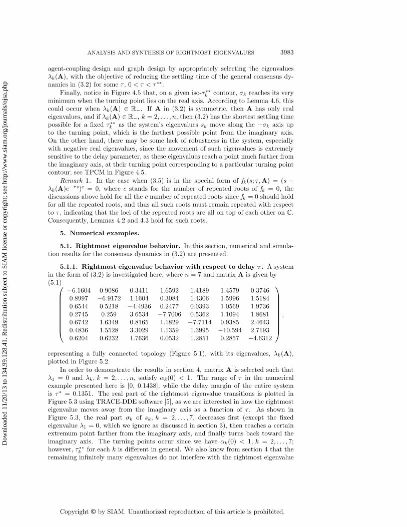
5.1.1. Rightmost eigenvalue behavior with respect to delay τ . A systemin the form of (3.2) is investigated here, where n = 7 and matrix A is given by(5.1)⎛

⎜⎜⎜⎜⎜⎜⎜⎜⎝

−6.1604 0.9086 0.3411 1.6592 1.4189 1.4579 0.37460.8997 −6.9172 1.1604 0.3084 1.4306 1.5996 1.51840.6544 0.5218 −4.4936 0.2477 0.0393 1.0569 1.97360.2745 0.259 3.6534 −7.7006 0.5362 1.1094 1.86810.6742 1.6349 0.8165 1.1829 −7.7114 0.9385 2.46430.4836 1.5528 3.3029 1.1359 1.3995 −10.594 2.71930.6204 0.6232 1.7636 0.0532 1.2851 0.2857 −4.6312

⎞⎟⎟⎟⎟⎟⎟⎟⎟⎠,

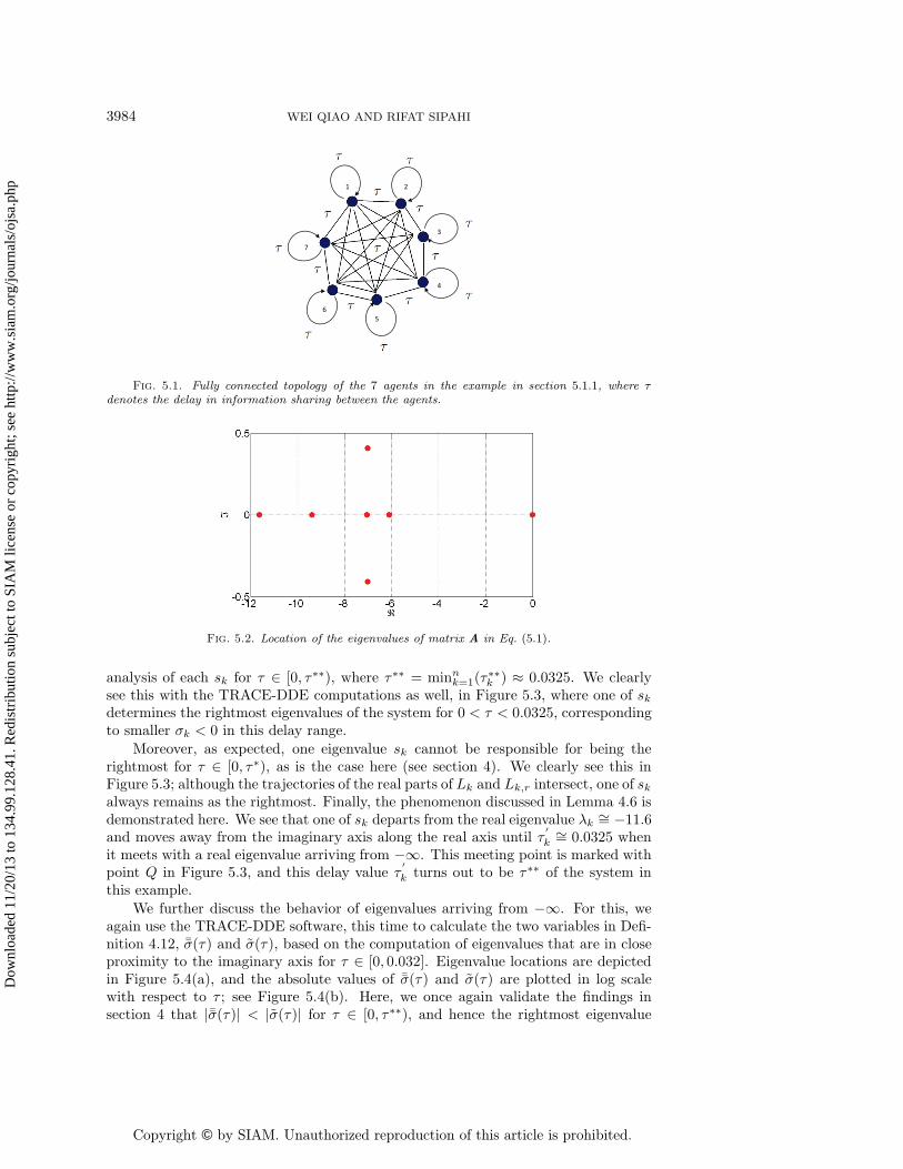
representing a fully connected topology (Figure 5.1), with its eigenvalues, λk(A),plotted in Figure 5.2.

In order to demonstrate the results in section 4, matrix A is selected such thatλ1 = 0 and λk, k = 2, . . . , n, satisfy αk(0) < 1. The range of τ in the numericalexample presented here is [0, 0.1438], while the delay margin of the entire systemis τ∗ = 0.1351. The real part of the rightmost eigenvalue transitions is plotted inFigure 5.3 using TRACE-DDE software [5], as we are interested in how the rightmosteigenvalue moves away from the imaginary axis as a function of τ . As shown inFigure 5.3, the real part σk of sk, k = 2, . . . , 7, decreases first (except the fixedeigenvalue λ1 = 0, which we ignore as discussed in section 3), then reaches a certainextremum point farther from the imaginary axis, and finally turns back toward theimaginary axis. The turning points occur since we have αk(0) < 1, k = 2, . . . , 7;however, τ∗∗k for each k is different in general. We also know from section 4 that theremaining infinitely many eigenvalues do not interfere with the rightmost eigenvalue

Dow

nloa

ded

11/2

0/13

to 1

34.9

9.12

8.41

. Red

istr

ibut

ion

subj

ect t

o SI

AM

lice

nse

or c

opyr

ight

; see

http

://w

ww

.sia

m.o

rg/jo

urna

ls/o

jsa.

php



1 2

7

6 5

4

3

Fig. 5.1. Fully connected topology of the 7 agents in the example in section 5.1.1, where τdenotes the delay in information sharing between the agents.

Fig. 5.2. Location of the eigenvalues of matrix A in Eq. (5.1).

analysis of each sk for τ ∈ [0, τ∗∗), where τ∗∗ = minnk=1(τ

∗∗k ) ≈ 0.0325. We clearly

see this with the TRACE-DDE computations as well, in Figure 5.3, where one of skdetermines the rightmost eigenvalues of the system for 0 < τ < 0.0325, correspondingto smaller σk < 0 in this delay range.

Moreover, as expected, one eigenvalue sk cannot be responsible for being therightmost for τ ∈ [0, τ∗), as is the case here (see section 4). We clearly see this inFigure 5.3; although the trajectories of the real parts of Lk and Lk,r intersect, one of skalways remains as the rightmost. Finally, the phenomenon discussed in Lemma 4.6 isdemonstrated here. We see that one of sk departs from the real eigenvalue λk ∼= −11.6and moves away from the imaginary axis along the real axis until τ

′k∼= 0.0325 when

it meets with a real eigenvalue arriving from −∞. This meeting point is marked withpoint Q in Figure 5.3, and this delay value τ

′k turns out to be τ∗∗ of the system in

this example.

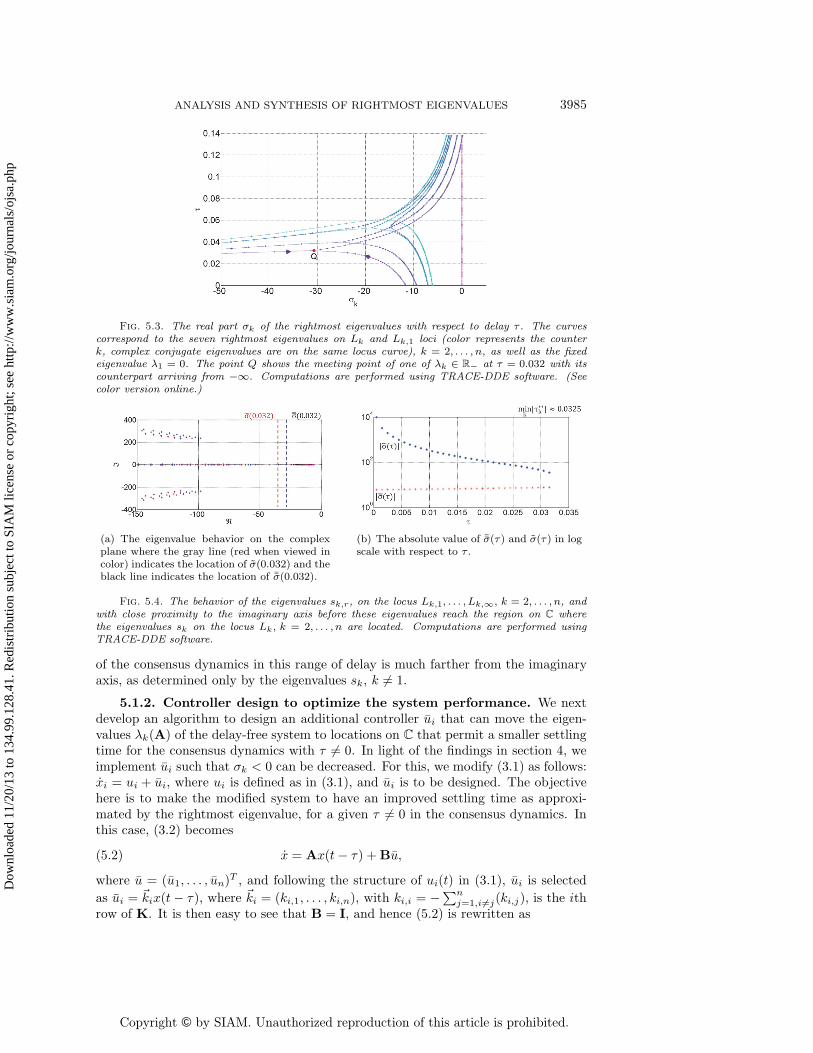
We further discuss the behavior of eigenvalues arriving from −∞. For this, weagain use the TRACE-DDE software, this time to calculate the two variables in Defi-nition 4.12, ¯σ(τ) and σ(τ), based on the computation of eigenvalues that are in closeproximity to the imaginary axis for τ ∈ [0, 0.032]. Eigenvalue locations are depictedin Figure 5.4(a), and the absolute values of ¯σ(τ) and σ(τ) are plotted in log scalewith respect to τ ; see Figure 5.4(b). Here, we once again validate the findings insection 4 that |¯σ(τ)| < |σ(τ)| for τ ∈ [0, τ∗∗), and hence the rightmost eigenvalue

Dow

nloa

ded

11/2

0/13

to 1

34.9

9.12

8.41

. Red

istr

ibut

ion

subj

ect t

o SI

AM

lice

nse

or c

opyr

ight

; see

http

://w

ww

.sia

m.o

rg/jo

urna

ls/o

jsa.

php



Fig. 5.3. The real part σk of the rightmost eigenvalues with respect to delay τ . The curvescorrespond to the seven rightmost eigenvalues on Lk and Lk,1 loci (color represents the counterk, complex conjugate eigenvalues are on the same locus curve), k = 2, . . . , n, as well as the fixedeigenvalue λ1 = 0. The point Q shows the meeting point of one of λk ∈ R− at τ = 0.032 with itscounterpart arriving from −∞. Computations are performed using TRACE-DDE software. (Seecolor version online.)

(a) The eigenvalue behavior on the complexplane where the gray line (red when viewed incolor) indicates the location of σ(0.032) and theblack line indicates the location of ¯σ(0.032).

(b) The absolute value of ¯σ(τ) and σ(τ) in logscale with respect to τ .

Fig. 5.4. The behavior of the eigenvalues sk,r, on the locus Lk,1, . . . , Lk,∞, k = 2, . . . , n, andwith close proximity to the imaginary axis before these eigenvalues reach the region on C wherethe eigenvalues sk on the locus Lk , k = 2, . . . , n are located. Computations are performed usingTRACE-DDE software.

of the consensus dynamics in this range of delay is much farther from the imaginaryaxis, as determined only by the eigenvalues sk, k �= 1.

5.1.2. Controller design to optimize the system performance. We nextdevelop an algorithm to design an additional controller ui that can move the eigen-values λk(A) of the delay-free system to locations on C that permit a smaller settlingtime for the consensus dynamics with τ �= 0. In light of the findings in section 4, weimplement ui such that σk < 0 can be decreased. For this, we modify (3.1) as follows:xi = ui + ui, where ui is defined as in (3.1), and ui is to be designed. The objectivehere is to make the modified system to have an improved settling time as approxi-mated by the rightmost eigenvalue, for a given τ �= 0 in the consensus dynamics. Inthis case, (3.2) becomes

(5.2) x = Ax(t− τ) +Bu,

where u = (u1, . . . , un)T , and following the structure of ui(t) in (3.1), ui is selected

as ui = �kix(t− τ), where �ki = (ki,1, . . . , ki,n), with ki,i = −∑nj=1,i�=j(ki,j), is the ith

row of K. It is then easy to see that B = I, and hence (5.2) is rewritten as

Dow

nloa

ded

11/2

0/13

to 1

34.9

9.12

8.41

. Red

istr

ibut

ion

subj

ect t

o SI

AM

lice

nse

or c

opyr

ight

; see

http

://w

ww

.sia

m.o

rg/jo

urna

ls/o

jsa.

php



(5.3) x = (A+K)x(t− τ),

which recovers the same type of system as in (3.2).Based on the discussions above, a controller design procedure can be developed

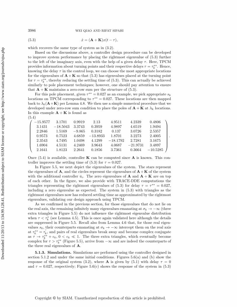
to improve system performance by placing the rightmost eigenvalue of (5.3) furtherto the left of the imaginary axis, even with the help of a given delay τ . Here, TPCMprovides information about turning points and their respective delays τ = τ∗∗k . Hence,knowing the delay τ in the control loop, we can choose the most appropriate locationsfor the eigenvalues of A+K so that (5.3) has eigenvalues placed at the turning pointfor τ = τ∗∗k , thereby reducing the settling time of (5.3). This can actually be achievedsimilarly to pole placement techniques; however, one should pay attention to ensurethat A+K maintains a zero-row sum per the structure of (5.3).

For this pole placement, given τ∗∗ = 0.027 as an example, we pick appropriate sklocations on TPCM corresponding to τ∗∗ = 0.027. These locations are then mappedback to λk(A+K) per Lemma 4.8. We then use a simple numerical procedure that wedeveloped under zero-row sum condition to place the poles of A+K at λk locations.In this example A+K is found as(5.4)⎛⎜⎜⎜⎜⎜⎜⎜⎜⎝

−15.9577 3.1701 0.9919 2.13 4.9511 4.2339 0.48063.1431 −18.5043 3.3743 0.3959 4.9897 4.6519 1.94942.2846 1.5169 −9.865 0.3182 0.137 3.0726 2.53570.9573 0.7523 4.6859 −13.8933 1.8701 3.2273 2.40052.3543 4.7495 1.0498 4.1299 −18.1792 2.7281 3.16751.6904 4.5131 4.2469 3.9643 4.0687 −21.9731 3.48972.1641 1.8123 2.2641 0.1856 3.7361 0.3664 −10.5285

⎞⎟⎟⎟⎟⎟⎟⎟⎟⎠.

Once (5.4) is available, controller K can be computed since A is known. This con-troller improves the settling time of (5.3) for τ = 0.027.

In Figure 5.5, we next depict the eigenvalues of the system. The stars representthe eigenvalues of A, and the circles represent the eigenvalues of A+K of the systemwith the additional controller ui. The zero eigenvalues of A and A + K are on topof each other. In the figure, we also provide with TRACE-DDE computations thetriangles representing the rightmost eigenvalues of (5.3) for delay τ = τ∗∗ = 0.027,including a zero eigenvalue as expected. The system in (5.3) with triangles as therightmost eigenvalues now has reduced settling time as approximated by the rightmosteigenvalues, validating our design approach using TPCM.

As we confirmed in the previous section, for those eigenvalues that do not lie onthe real axis, the remaining infinitely many eigenvalues emanating at σk → −∞ (threeextra triangles in Figure 5.5) do not influence the rightmost eigenvalue distributionwhen τ < τ∗k (see Lemma 4.5). This is once again validated here although the detailsare suppressed in Figure 5.5. Recall also from Lemma 4.6 that, for those real eigen-values sk, their counterparts emanating at σk → −∞ intercept them on the real axisat τ∗∗k = τ

′k, and pairs of real eigenvalues break away and become complex conjugate

as τ → τ∗∗k + εk, 0 < εk 1. The three extra triangles, which eventually becomecomplex for τ > τ∗∗k (Figure 5.5), arrive from −∞ and are indeed the counterparts ofthe three real eigenvalues of A.

5.1.3. Simulations. Simulations are performed using the controller designed insection 5.1.2 and under the same initial conditions. Figures 5.6(a) and (b) show theresponse of the original system (3.2), where A is given by (5.1) with delay τ = 0and τ = 0.027, respectively; Figure 5.6(c) shows the response of the system in (5.3)

Dow

nloa

ded

11/2

0/13

to 1

34.9

9.12

8.41

. Red

istr

ibut

ion

subj

ect t

o SI

AM

lice

nse

or c

opyr

ight

; see

http

://w

ww

.sia

m.o

rg/jo

urna

ls/o

jsa.

php



Fig. 5.5. Stars represent the eigenvalue of A (i.e., sk(τ = 0) = λk(A)), circles represent theeigenvalues of A + K (i.e., sk(τ = 0) = λk(A + K)), and the triangles represent the eigenvalueswith delay τ = τ∗∗k = 0.027 in (5.3) (i.e., sk and sk,r at τ = τ∗∗k ) computed by TRACE-DDE. Threeextra triangles arrive from σk → −∞ for τ → 0+ and are the counterparts of three real eigenvaluessk arriving from λk ∈ R− for τ → 0+. On the origin, we have a circle, a triangle, and a star symbolrepresenting λ1 = 0 eigenvalue in all three scenarios.

(a) Simulation result of the system (3.2) whereA is given by (5.1) with delay τ = 0.

(b) Simulation result of the system (3.2) whereA is given by (5.1) with delay τ = 0.027.

(c) Simulation result of system (5.3) where A+K is given by (5.4) with delay τ = 0.

(d) Simulation result of the system in (5.3)where A + K is given by (5.4) with delayτ = 0.027.

Fig. 5.6. Simulation results of the system with/without controller and time delay. Initial condi-tions are randomly generated in [0, 1] using MATLAB, and are kept the same in all the simulations.

with delay τ = 0, and finally, Figure 5.6(d) shows the behavior of (5.3) with delayτ = 0.027, where A+K is given by (5.4). Clearly, the simulation results are consistentwith those predicted in the analytical and numerical results, and the settling time isreduced from 0.6 sec in Figure 5.6(a) to 0.22 sec in Figure 5.6(d), even if the responseof the latter starts only after τ = 0.027 sec elapses.

Dow

nloa

ded

11/2

0/13

to 1

34.9

9.12

8.41

. Red

istr

ibut

ion

subj

ect t

o SI

AM

lice

nse

or c

opyr

ight

; see

http

://w

ww

.sia

m.o

rg/jo

urna

ls/o

jsa.

php



(a) Mean and standard deviation of |σmax(τ =τ∗∗)| for 50 trials for each Γ = τ2 − τ1.

(b) Mean and standard deviation of |σmax(τ =τ∗∗)| for 50 trials for each τ2/τ1.

Fig. 5.7. Mean and standard deviation of |σmax(τ = τ∗∗)| for 50 trials. In each trial, τ∗∗represents a different combination of τ1 and τ2 at the turning point, and the turning points atτ = τ∗∗ are in general different at each trial.

5.2. Rightmost eigenvalue behavior with two nonidentical delays. In thecase when the delays between the agents are not identical, an analytically tractableanalysis of rightmost eigenvalues is not possible. To investigate such problems, oneneeds to refer to numerical analysis tools. In this section, we consider examples inwhich two different delays τ1 and τ2 exist in the dynamics. We investigate the arisingproblems with the help of the TRACE-DDE tool [5].

For the system with two nonidentical delays, (3.2) modifies to

(5.5) x(t) = A1x(t− τ1) +A2x(t − τ2),

where A1 + A2 has zero row sum, and the agents are fully connected. In this sub-section, all the nondiagonal entries of either A1 or A2 are randomized between 0 and1 selected from a uniform distribution, and A1 and A2 are complementary. In otherwords, for all A1[i, k] �= 0, i, k = 1, . . . , n, we have A2[i, k] = 0, i, k = 1, . . . , n, andvice versa. The probability of A1[i, k] �= 0 is equal to 60%, while the probability ofA2[i, k] �= 0 is equal to 40%.

We take a 5 × 5 system and calculate, using TRACE-DDE, the real part of therightmost eigenvalues, σmax when a turning point is registered at some τ = τ∗∗,while using the difference Γ = τ2 − τ1 as a parameter. For each Γ, we randomizeA1 and A2 50 times, ensuring zero row sum, and then compute σmax at the turningpoint (where τ∗∗ = 0 if turning point does not exist), which can be different in eachtrial. As Γ varies from 0 to 1 sec, we also show the mean and standard deviation of|σmax(τ = τ∗∗)| with respect to Γ; see Figure 5.7(a). Similar analysis is repeated alsofor τ2/τ1 ranging from 1 to 2.5; see Figure 5.7(b).

The above results indicate that the mean of the real part of the rightmost eigen-value at the turning point is approaching the imaginary axis as the differences betweenτ1 and τ2 increase. In other words, nonhomogeneous delays add negative effect onthe system performance in terms of the rightmost eigenvalue location at the turn-ing point. However, this cannot be generalized for all delay differences due to thevariance in the results. For instance, as shown in Figures 5.8(a) and (b) for a singletrial, the rightmost eigenvalue at the turning point can shift away from the imaginaryaxis, depending on fixed but randomized matrices A1 and A2, and as delay differenceincreases within a certain range, indicating reduced settling time. Finally, note that|σmax(τ = τ∗∗)| = 1.85 for (τ2 − τ1) ∈ [0.65, 1] shown in Figure 5.8(a) stands for thecase where the rightmost eigenvalue goes directly toward the imaginary axis as τ1

Dow

nloa

ded

11/2

0/13

to 1

34.9

9.12

8.41

. Red

istr

ibut

ion

subj

ect t

o SI

AM

lice

nse

or c

opyr

ight

; see

http

://w

ww

.sia

m.o

rg/jo

urna

ls/o

jsa.

php



(a) The rightmost eigenvalue at turning pointwith respect to Γ = τ2 − τ1 for one trial.

(b) The rightmost eigenvalue at turning pointwith respect to τ2/τ1 for one trial.

Fig. 5.8. The rightmost eigenvalue at turning point for one trial as delay difference in dynamics(5.5) increases. Note that |σmax(τ = τ∗∗)| = 1.85 for (τ2 − τ1) ∈ [0.65, 1] shown in (a) stands forthe case where the rightmost eigenvalue goes directly toward the imaginary axis as τ1 changes from0 to 0+, and hence τ∗∗ = 0 and in this case |σmax(τ∗∗)| = mink=2,...,n |�(λk)|.

changes from 0 to 0+. In such cases, we set τ∗∗ = 0, and the rightmost root is locatedwhere λk(A) is located.

6. Conclusions and future research. Rightmost eigenvalue behavior of a classof LTI consensus dynamics with a fixed graph Laplacian is investigated where a singledelay exists in all communication channels between coupled agents. We develop ananalytical approach to investigate this behavior, which is associated with an infinite-dimensional eigenvalue problem, to ultimately reveal the correlation between the finitenumber of graph Laplacian eigenvalues and the stabilizing effects of delays. Specifi-cally, we show here analytically that the rightmost eigenvalue can be placed fartherfrom the imaginary axis of the complex plane for larger delays, under certain condi-tions of the graph Laplacian eigenvalues. This indicates that with proper controllerdesign and topology design, the rightmost eigenvalues of the infinite-dimensionalconsensus dynamics can be shifted to a region on the complex plane, favoring re-duced settling time for a nonzero delay. Numerical examples and simulation resultsconfirm and demonstrate the stabilization effects of delays where the consensus dy-namics with nonzero time delay has improved transient response compared to thedelay-free case. Since analytical study of rightmost eigenvalues for the multiple/nonidentical delay case is not feasible, numerical analysis is also utilized, specificallyon examples with two delays to explore the effects of delay difference/mismatch inthe dynamics. Some possible directions for future research could include further ex-tensions to nonidentical delay cases, mathematical developments for control designto manipulate the graph Laplacian eigenvalues as well as the graphs themselves, andconsideration of distributed delays in the controller.

REFERENCES

[1] C. T. Abdallah, N. Alluri, J. D. Birdwell, J. Chiasson, V. Chupryna, Z. Tang, and

T. Wang, Linear time delay model for studying load balancing instabilities in parallelcomputations, Internat. J. Systems Sci., 34 (2003), pp. 563–573.

[2] F. M. Atay ed., Complex Time-Delay Systems, Springer-Verlag, Berlin, 2010.[3] R. Bellman and K. L. Cooke, Differential-Difference Equations, Academic Press, New York,

US, 1963.[4] D. Breda, On characteristic roots and stability charts of delay differential equations, Internat.

J. Robust Nonlinear Control, 22 (2012), pp. 892–917.

Dow

nloa

ded

11/2

0/13

to 1

34.9

9.12

8.41

. Red

istr

ibut

ion

subj

ect t

o SI

AM

lice

nse

or c

opyr

ight

; see

http

://w

ww

.sia

m.o

rg/jo

urna

ls/o

jsa.

php



[5] D. Breda, S. Maset, and R. Vermiglio, TRACE-DDE: A tool for robust analysis and char-acteristic equations for delay differential equations, in Topics in Time Delay Systems,J. Loiseau, W. Michiels, S.-I. Niculescu, and R. Sipahi, eds., Lecture Notes in Control andInform. Sci. 388, Springer, Berlin, Heidelberg, 2009, pp. 145–155.

[6] J. Chen, G. Gu, and C. N. Nett, A new method for computing delay margins for stability oflinear delay systems, Systems Control Lett., 26 (1995), pp. 107–117.

[7] F. Chung, Spectral Graph Theory, Amer. Math. Soc., Providence, RI, 1997.[8] K. L. Cooke and P. van den Driessche, On zeros of some transcendental equations, Funkcial.

Ekvac., 29 (1986), pp. 77–90.[9] R. Datko, A procedure for determination of the exponential stability of certain differential-

difference equations, Quart. Appl. Math., 36 (1978), pp. 279–292.[10] M. Dhamala, V. K. Jirsa, and M. Ding, Enhancement of neural synchrony by time delay,

Phys. Rev. Lett., 92 (2004), 074104.[11] J. A. Fax and R. M. Murray, Information flow and cooperative control of vehicle formations,

IEEE Trans. Automat. Control, 49 (2004), pp. 1465–1476.[12] W. Fulton, Algebraic Curves: An Introduction to Algebraic Geometry, Addison-Wesley

Publishing Company, Advanced Book Program, Redwood City, CA, 1989.[13] K. Gu, V. L. Kharitonov, and J. Chen, Stability of Time-Delay Systems, Birkhauser, Boston,

2003.[14] K. Gu, S.-I. Niculescu, and J. Chen, On stability crossing curves for general systems with

two delays, J. Math. Anal. Appl., 311 (2005), pp. 231–253.[15] J. K. Hale and W. Huang, Global geometry of the stable regions for two delay differential

equations, J. Math. Anal. Appl., 178 (1993), pp. 344–362.[16] D. Helbing, Traffic and related self-driven many-particle systems, Rev. Modern Phys., 73

(2001), pp. 1067–141.[17] D. Helbing, S. Lammer, T. Seidel, P. Seba, and T. P�latkowski, Physics, stability and

dynamics of supply networks, Phys. Rev. E, 70 (2004), 066116.[18] S. Hod, Analytic treatment of the network synchronization problem with time delays, Phys.

Rev. Lett., 105 (2010), 208701.[19] P. F. Hokayem and M. W. Spong, Bilateral teleoperation: An historical survey, Automatica,

42 (2006), pp. 2035–2057.[20] D. Hunt, G. Korniss, and B. K. Szymanski, Network synchronization in a noisy environment

with time delays: Fundamental limits and trade-offs, Phys. Rev. Lett., 105 (2010), 068701.[21] D. Hunt, G. Korniss, and B. K. Szymanski, The impact of competing time delays in coupled

stochastic systems, Phys. Lett. A, 375 (2011), pp. 880–885.[22] E. Jarlebring, Computing the stability region in delay-space of a TDS using polynomial eigen-

problems, in Proceedings of the 6th IFAC Workshop on Time-Delay Systems, L’Aquila,Italy, 2006, pp. 296–301.

[23] E. Jarlebring, Critical delays and polynomial eigenvalue problems, J. Comput. Appl. Math.,224 (2009), pp. 296–306.

[24] B. Kelleher, C. Bonatto, P. Skoda, S. P. Hegarty, and G. Huyet, Excitation regenerationin delay-coupled oscillators, Phys. Rev. E, 81 (2010), 036204.

[25] J. J. Loiseau, W. Michiels, S.-I. Niculescu, and R. Sipahi, eds., Topics in Time DelaySystems Analysis, Algorithms and Control, Springer-Verlag, Berlin, 2009.

[26] J. Lu, D. W. C. Ho, and J. Kurths, Consensus over directed static networks with arbitraryfinite communication delays, Phys. Rev. E, 80 (2009), 066121.

[27] J. E. Marshall, H. Gorecki, K. Walton, and A. Korytowski, Time-Delay Systems: Sta-bility and Performance Criteria with Applications, Ellis Horwood, New York, 1992.

[28] R. Merris, Laplacian matrices of graphs: A survey, Linear Algebra Appl., 197/198 (1994),pp. 143–176.

[29] W. Michiels, K. Engelborghs, P. Vansevenant, and D. Roose, Continuous pole placementmethod for delay equations, Automatica, 38 (2002), pp. 747–761.

[30] W. Michiels and S.-I. Niculescu, Stability and Stabilization of Time-Delay Systems: AnEigenvalue-Based Approach, Adv. Des. Control 12, SIAM, Philadelphia, 2007.

[31] W. Michiels, T. Vyhlidal, and P. Zıtek, Control design for time-delay systems based onquasi-direct pole placement, J. Process Control, 20 (2010), pp. 337–343.

[32] S.-I. Niculescu, Delay Effects on Stability: A Robust Control Approach, Lecture Notes inControl and Inform. Sci. 269, Springer-Verlag, Berlin, 2001.

[33] S.-I. Niculescu and W. Michiels, Stabilizing a chain of integrators using multiple delays,IEEE Trans. Automat. Control, 49 (2004), pp. 802–807.

[34] S. Nosrati, M. Shafiee, and M. B. Menhaj, Synthesis and analysis of robust dynamic lin-ear protocols for dynamic average consensus estimators, Control Theory Appl., 3 (2009),pp. 1499–1516.

Dow

nloa

ded

11/2

0/13

to 1

34.9

9.12

8.41

. Red

istr

ibut

ion

subj

ect t

o SI

AM

lice

nse

or c

opyr

ight

; see

http

://w

ww

.sia

m.o

rg/jo

urna

ls/o

jsa.

php



[35] K. Ogata, Morden Control Engineering, Prentice Hall, Upper Saddle River, NJ, 2002.[36] R. Olfati-Saber, Ultrafast consensus in small-world networks, in Proceedings of the American

Control Conference, Portland, OR, 2005, pp. 2371–2378.[37] R. Olfati-Saber and R. M. Murray, Consensus problems in networks of agents with switch-

ing topology and time-delays, IEEE Trans. Automat. Control, 49 (2004), pp. 1520–1533.[38] N. Olgac and R. Sipahi, An exact method for the stability analysis of time delayed LTI

systems, IEEE Trans. Automat. Control, 47 (2002), pp. 793–797.[39] N. Olgac, R. Sipahi, and A. F. Ergenc, ‘Delay scheduling’, an unconventional use of time

delay for trajectory tracking, Mechatronics, 17 (2007), pp. 199–206.[40] G. Orosz, R. Wilson, and G. Stepan, Traffic jams: Dynamics and control, Philos. Trans.

R. Soc. Lon. Ser. A Math. Phys. Eng., 368 (2010), pp. 4455–4479.[41] M. Porfiri and F. Fiorilli, Global pulse synchronization of chaotic oscillators through fast-

switching: Theory and experiments, Chaos Solitons Fractals, 41 (2009), pp. 245–262.[42] M. Porfiri, D. G. Roberson, and D. J. Stilwell, Tracking and formation control of

multiple autonomous agents: A two-level consensus approach, Automatica, 43 (2007),pp. 1318–1328.

[43] W. Qiao and R. Sipahi, Dependence of delay margin on network topology: Single delay case, inProceedings of the 9th IFAC Workshop on Time Delay Systems, Prague, Czech Republic,2010, pp. 93–98.

[44] W. Qiao and R. Sipahi, Responsible eigenvalue approach for stability analysis and con-trol design of a single-delay large-scale system with random coupling strengths, in Pro-ceedings of the ASME 3rd Dynamic Systems and Control Conference, Cambridge, MA,2010, pp. 531–537.

[45] W. Qiao and R. Sipahi, Responsible eigenvalue control for creating autonomy in coupled sys-tems with delays, in Proceedings of the ASME Dynamic Systems and Control Conference,Arlington, VA, 2011.

[46] W. Qiao and R. Sipahi, Rules and limitations of building delay-tolerant topologies for coupledsystems, Phys. Rev. E, 85 (2012), 016104.

[47] W. Ren, R. W. Beard, and E. M. Atkins, A survey of consensus problems in multi-agentcoordination, in Proceedings of the American Control Conference, Portland, OR, 2005.

[48] A. Schollig, U. Munz, and F. Allgower, Topology-dependent stability of a network ofdynamical systems with communication delays, in Proceedings of the European ControlConference, Kos, Greece, 2007, pp. 1197–1202.

[49] R. Sipahi and A. Acar, Stability analysis of three-agent consensus dynamics with fixed topologyand three non-identical delays, in Proceedings of the ASME Dynamic Systems and ControlConference, Ann Arbor, MI, 2008.

[50] R. Sipahi, F. M. Atay, and S.-I. Niculescu, Stability of traffic flow behavior with distributeddelays modeling the memory effects of the drivers, SIAM J. Appl. Math., 68 (2007),pp. 738–759.

[51] R. Sipahi and I. I. Delice, Extraction of 3D stability switching hypersurfaces of a time delaysystem with multiple fixed delays, Automatica, 45 (2009), pp. 1449–1454.

[52] R. Sipahi and I. I. Delice, Advanced clustering with frequency sweeping methodology for thestability analysis of multiple time-delay systems, IEEE Trans. Automat. Control, 56 (2011),pp. 467–472.

[53] R. Sipahi and S.-I. Niculescu, Deterministic time-delayed traffic flow models: A Survey, inComplex Time-Delay Systems, Springer-Verlag, Berlin, 2010, pp. 297–322.

[54] R. Sipahi, S.-I. Niculescu, C. T. Abdallah, W. Michiels, and K. Gu, Stability and stabi-lization of systems with time delay, limitations and opportunities, IEEE Control SystemsMagazine, 31 (2011), pp. 38–65.

[55] R. Sipahi and N. Olgac, Complete stability robustness of third-order LTI multiple time-delaysystems, Automatica, 41 (2005), pp. 1413–1422.

[56] R. Sipahi and N. Olgac, Stability robustness of retarded LTI systems with single delay andexhaustive determination of their imaginary spectra, SIAM J. Control Optim., 45 (2006),pp. 1680–1696.

[57] R. Sipahi and W. Qiao, Responsible eigenvalue concept for the stability of a class of single-delay consensus dynamics with fixed topology, Control Theory Appl., 5 (2011), pp. 622–629.

[58] R. Sipahi and W. Qiao, Erratum for ‘responsible eigenvalue concept for the stability of a classof single-delay consensus dynamics with fixed topology’, Control Theory Appl., 6 (2012),p. 1154.

[59] F. K. Skinner, H. Bazzazi, and S. A. Campbell, Two-cell to n-cell heterogeneous, inhibitorynetworks: Precise linking of multistable and coherent properties, J. Comput. Neurosci., 18(2005), pp. 343–352.

Dow

nloa

ded

11/2

0/13

to 1

34.9

9.12

8.41

. Red

istr

ibut

ion

subj

ect t

o SI

AM

lice

nse

or c

opyr

ight

; see

http

://w

ww

.sia

m.o

rg/jo

urna

ls/o

jsa.

php



[60] G. Stepan, Retarded Dynamical Systems: Stability and Characteristic Functions, Pitman Res.Notes Math. Ser. 210, Longman Scientific & Technical, John Wiley & Sons, Inc., New York,1989.

[61] O. Toker and H. Ozbay, Complexity issues in robust stability of linear delay-differentialsystems, Math. Control Signals Systems, 9 (1996), pp. 386–400.

[62] K. Verheyden, T. Luzyanina, and D. Roose, Efficient computation of characteristic rootsof delay differential equations using LMS methods, J. Comput. Appl. Math., 214 (2008),pp. 209–226.

[63] T. Vyhlidal and P. Zıtek, Mapping based algorithm for large-scale computation of quasi-polynomial zeros, IEEE Trans. Automat. Control, 54 (2009), pp. 171–177.

[64] Z. H. Wang and H. Y. Hu, Calculation of the rightmost characteristic root of retarded time-delay systems via Lambert W function, J. Sound Vibration, 318 (2008), pp. 757–767.

[65] S. Yi, S. Duan, P. Nelson, and A. Ulsoy, The Lambert W function approach to time delaysystems and the LambertW-DDE toolbox, in Proceedings of the 10th IFAC Workshop onTime Delay Systems, Boston, MA, 2012, pp. 114–119.

Dow

nloa

ded

11/2

0/13

to 1

34.9

9.12

8.41

. Red

istr

ibut

ion

subj

ect t

o SI

AM

lice

nse

or c

opyr

ight

; see

http

://w

ww

.sia

m.o

rg/jo

urna

ls/o

jsa.

php

a linear time-invariant consensus dynamics with homogeneous delays: analytical study and synthesis...

Documents