Philips tech. Rev. 40, 329-337,1982, No. 11/12 329

A linear d.c. motor with permanent magnets

L. Honds and K. H. Meyer

Take two permanent magnets and three iron bars and wind copper wire around one of thebars. This is the idea behind the linear motor designed at Philips Forschungslaboratorium inAachen and described in the article below. The method of calculating the characteristics of themotor is just as simple. Measurements and calculations with MAGGY - a comprehensiveprogram package for computing magnetic fields - demonstrate that the method of calcula-tion yields the right results. The practical value of this kind of motor is demonstrated by itsapplication in the 12channel Transokomp 250 multipoint recorder developed by the PhilipsScience and Industry Division.

Introduetion

Linear movements are frequently used in engineer-ing. They are commonly produced by a drive mechan-ism operated by a rotor-type electric motor, since theseare widely available commercially in many versions.However, the conversion mechanism introduces extrafriction, takes up space and also increases the movingmass.

For certain applications, it is usual to produce alinear motion directly by means of a linear motor. Theelectromagnet with a movable armature, for example,is used in different variations in electric bells, in relays,in vibrators and so on. Although linear machines ofthis type can produce a considerable force, the strokeis limited. Also, the force is not the same for thevarious positions of the armature.

Other types of linear motors are suitable for trac-tion applications. Linear machines of this type haveattracted attention again because of the recent devel-opments associated with passenger transport in denselypopulated urban areas. Such machines are required tohave an 'unlimited' stroke and their force should notvary significantly during the displacement. Althoughthe various electromechanical principles of rotaryelectrical machines still apply here [11, the machinesused are usually linear induction motors or linear syn-chronous motors.

The type of linear motor we shall discuss in thisarticle has a stroke varying between that of the twotypes mentioned above. In practice the stroke is limitedto about half a metre. The force is virtually indepen-dent of the displacement. No current has to be sup-

Ing. L. Honds and Dr Ing. K. H. Meyer are with Philips GmbHForschungs/aboratorium Aachen, Aachen, West Germany.

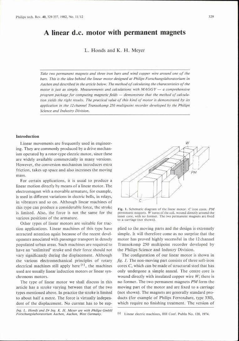
w

Fig. 1. Schematic diagram of the linear motor. C iron cores. PMpermanent magnets. W turns of the coil, wound directly around theinner core, with no former. The two permanent magnets are fixedto a carriage (not shown).

plied to the moving parts and the design is extremelysimple. It will therefore come as no surprise that themotor has proved highly successful in the 12 channelTransokomp 250 multipoint recorder developed bythe Philips Science and Industry Division.

The configuration of our linear motor is shown infig. 1. The non-moving part consists of three soft-ironcores C, which can be made of structural steel that hasonly undergone a simple anneal. The centre core iswound directly with insulated copper wire W; there isno former. The two permanent magnets PM form themoving part of the motor and are fixed to a carriage(not shown). The magnets are generally standard pro-ducts (for example of Philips Ferroxdure, type 330),which require no finishing treatment. The version of

[11 Linear electric machines, lEE Conf. Publn No. 120, 1974.

330 L. HONDS and K. H. MEYER Philips tech. Rev. 40, No. 11/12

the motor used in the recorder gives a force of 2 N(constant to within 51170)over a stroke of 250 mm. Thecross-section of this motor is 67 x 29 mm, and in thestationary state about 7 W is dissipated in the coil at aforce of 2 N.

Several variations of the version shown in fig. 1 canbe made. It is possible, for example, to 'halve' themotor, leaving only one permanent magnet and twoiron cores. The magnet can also be stationary, withthe coil moving. The current in that case, however,must be supplied by means of flexible wires or carbonbrushes. The method of calculation used for thesearrangements is almost identical, and we shall there-fore confine ourselves to the configuration given infig. 1.

First we shall explain how the force on the perma-nent magnets can be calculated. We shall then indicatethe value to which the current in the coil has to belimited to prevent saturation of the iron of the cores.Next, we shall give the graphic results of calculationsmade with the computer program MAGGY. Finallywe shall show how the motor design can be optimizedfor a particular application, and we shall give theresults of measurements on the motor used in theTransokornp 250.

Calculation of the force on the permanent magnets

To calculate the force acting on the permanentmagnets we start by considering the energy, as in cal-culating the torque acting on the permanent-magnetrotor of a synchronous electric motor [21. In our casewe then arrive at the following general equation [31

for the resultant force F on the permanent magnets:

d<PcM d WM 1 2 dLcF=I-- --- +-1 --

dp dp 2 dp'

where I is the current in the coil, <PCM is the flux link-age produced by integrating the flux from the per-manent magnets for each winding over the length ofthe coil, p is the coordinate defining the position ofthe permanent magnets, WM is the magnetic fieldenergy due to the permanent magnets, and Lc is theinductance of the coil; see jig. 2.

In equation (1) the second term on the right-handside is equal to zero, because WM does not depend onthe position of the magnets. We assume here that thereturn field of flux density Bo is uniform and thatthe stray field of flux density BOE does not depend onthe position of the magnets either - provided that-I <p < I-/M, where IM is the length of the magnetsand 21 is the totallength of the cores. If we assume inaddition that the relative perrneability of the materialof the permanent magnets is equal to 1, then the third

term on the right-hand side of (1) is also equal to zero.Equation (1) can then be expressed more simply as

d<PcMF=I--

dp

Calculating the flux linkage <PCM and then differentia-

(2)

ting with respect to p we obtain

IM WF=I (BE + Bo) -- b,

I

where BE is the flux density of the effective field, w thenum ber of turns of the coil and b the dimension of the

(3)

cores perpendicular to the plane of the drawing; seefig. 2.

To determine <PCM we calculate the flux from the permanent mag-nets that is linked by wdx/21 turns of the coil and integrate the resultover the ranges -I ~x <p, p ~x <p+ IM and p + IM ~x < I. Forthe first range we have

p wdx<PCMl = f (<POE + 2(1 + x)b Bo) --,~ U

where <POE is the flux from the field of flux density BOE emerging atthe head ends of the inner core. The contribution from the secondrange to the flux linkage is

~M dx<PCM2= f {<PoE+2(1+p)bBo-2(X-P)bBE}2:':'_.

p UFor the third range the contribution to the flux linkage is:

I dxcfJCM3 = f {<POE + 2(1+p)bBo - 2/MbBE + 2(x-p-/M)bBo)2:':'_.

~M U(Strictly speaking the three integrals should also contain a contribu-tion from the stray field of flux density Bos at the sides (see fig. 3),but in fact this makes no contribution in equation (3) since Bos isindependent of the variable p.)

p(1)

Fig. 2. Quantities for calculating the flux linkage of the coil for thefield of the permanent magnets. BE flux density of the effective fieldin the air gaps between the permanent magnets and the inner core,Bo flux density of the return field between the cores, BOE fluxdensity of the stray field at the head ends. x coordinate in the longi-tudinal direction with x = 0 for the centre of the motor, p coor-dinate defining the position of the permanent magnets. I current inthe coil; the associated field is not shown. b height (not indicated)of the cores perpendicular to the plane of the drawing, IM length ofthe magnets, 2/length of the cores. F resultant force on the per-manent magnets.

Philips tech. Rev. 40, No. 11/12 LINEAR D.e. MOTOR 331

If we assume that the totallength 2/ of the motor islarge with respect to the length IM of the permanentmagnets, we can disregard the magnetic flux densityBo of the return field in comparison with the effectivemagnetic flux density BE, and equation (3) simplifies to

IMF= - wIBEb.

/

In the following we shall use equation (4) as our basisfor the force calculations. Although this means thatthe theoretical value calculated for the force is slightlytoo small, the error is approximately compensated by

c:::=::::::JcIlllIIllIlD

c=JC!IlII1IIIlDc:::=::::::J

V\Z\Z\Z\Z\Z\Z\Z\Z\Z~lIlIIII1IlJ

V\Z\Z\Z\Z\7\7\7\7\7~C!IIIlJIill))

Fig. 3. The magnetic field from the two permanent magnets, splitinto a number of subfields. These are approximated by uniformor two-dimensional fields and are thus easily calculated. BM fluxdensity of the field in the permanent magnets. dM thickness of themagnets. BMS flux density of the stray field around the magnets.Bos flux density of the stray field at the sides of the cores. See alsothe caption to fig. 2.

(4)

the error due to assuming an idealized linear relation-ship between flux density and field-strength in thematerials.

To calculate F from equation (4) it is necessary todetermine the effective flux density BE. This can bedone in a simple way by dividing the total magneticfield into a number of subfields that are easier to cal-culate. Fig. 3 shows how the three-dimensional mag-netic field of the permanent magnets can be split intoa number of uniform and two-dimensional fields. Thefield due to the current in the coil has not been in-cluded here and we have assumed that the permeabilityof the iron is infinitely large. The subfields are:- the field in the permanent magnets, of flux densityBM;- the stray field around the magnets, of flux densityBMS;- the effective field in the air gaps between the mag-nets and the inner core, of flux density BE;- the return field between the iron cores, of fluxdensity Bo;- the stray field at the two sides, of flux density Bos;- the stray field at the two head ends, of flux densityBOE.

The calculation of the effective field

In the calculations that follow we shall consistentlyconsider one half of the motor, consisting of one per-manent magnet and half the coil. Fig. 4 indicates howthe magnetic circuit with the coil not energized can berepresented by an electrical equivalent circuit withconstant-voltage source, resistances and currents.

The permanent magnet is the constant-voltage sourcein the equivalent circuit and delivers a magnetomotiveforce FM. This quantity has the unit A (amperes) and

Fig. 4. Electrical equivalent circuit for a half of the magnetic cir-cuit. AM, AMS,AE, Aa, Aas and AOEpermeances of the differentsubfields, as indicated in fig. 3. FM magnetomotive force, due toone of the permanent magnets. <PM, <PMS,<PE,<Po, <Pas and <POEmagnetic fluxes in the subfields of fig. 3.

[2] E. M. H. Kamerbeek, Electric motors, Philips tech. Rev. 33,215-234, 1973.

[3] This follows from equation (9) on page 223 of [2].

332 L. HONDS and K. H. MEYER Philips tech. Rev. 40, No. 11/12

is the product of the apparent coercive field-strengthHe*, see fig. 5, and the thickness di« of the magnet:

The currents in the circuit are represented by the mag-netic fluxes tP in Vs or Wb (webers). The permeancesA in H (henrys) of the magnetic resistances for a uni-form field are equal to

A = /-lo/-lrAld,

where A is the area perpendicular to the direction ofthe lines of force, d is the length in the direction of thelines of force, /-lo is the permeability of free space inHim and /-lris the relative permeability.

B

t

-H

Fig. 5. Part of the magnetization curve for the materialof the per-manent magnets. B magnetic flux density, H field-strength. B,remanent flux density, He coercive field-strength, He· apparentcoercive field-strength.

.1. .1.15 aa

Fig. 6. Idealized geometryof the lines of force. The outer four linesof force are arcs of a circle, the others are parts of an ellipse. Ideal-izations of this kind can be used for deriving simple expressions forthe permeance [41. In this case, with the dimensions indicated in thefigure, the permance cIA of an element dx is given by

cIA = Ilo [0.26 + ~ In (Ö ~ 2a)] dx,

where ö is the width of the air gap and a is the half-width of theinner core and the full width of each outer core.

AE, zlo and AM are easily calculated from equation(6). In determining AM the value of BrlHe* must betaken for the product/-lO/-lr;see fig. 5. The permeancesAMS, Aas and AaE can be calculated from simple ex-pressions that apply for idealized circular or ellipticallines of force [4]; see fig. 6. In this figure and in ourcalculations the half-width a of the inner core hasbeen taken equal to the width of the outer cores.[41 H. C. Roters, Electromagnetic devices, WHey,New York 1970.

(5)

All the permeances and the magnetomotive force inthe circuit of fig. 4 are therefore known. We can nowset up a number of equations in which the fluxes arethe unknowns and which we can solve for tPE:

(7)

(8)

(6)

tPE = tPa + tPas + tPaE

tPM = tPE + tPMS

tPMS tPE tPa + tPas + tPaE-- = - + -=--;__-=..:::....__-==-AMS AE Aa + Aas + AaE

tPas =FM _ tPM •AMS AM

If we put tPE = AMBE, with AM equal to the area ofthe poles of the permanent magnet and FMAM = BrAM(from (5) and (6», we have the following expressionfor the effective flux density:

(9)

(10)

B _ BrE-( 1 1)------ + - (AMs + AM) + 1Aa + Aas + AaE AE

(11)

Neglecting the effect of the stray fields, we haveAas = AaE = AMS = 0, and eq. (11) reduces to thesimpler relation:

BE =Br (12)

(_1_ + _1_) AM + 1Aa AE

The field in the cores

It was assumed above that when the subfields weresummed the flux density of the core iron was on thelinear part of the magnetization curve. To test thevalidity of this assumption, the flux density in thecores should be calculated. The field due to the cur-rent in the coil must then be taken into account aswell. We have already assumed that the inner core hastwice the cross-section of each of the outer cores. Theflux densities in the three cores are therefore identical.

First of all we calculate the effect of the permanentmagnet. Infig. 7a the fields in air are given for the casewhere the permanent magnet is in the extreme left-hand position, disregarding the stray fields. The fluxdensity BE of the effective field follows from (12). Theflux density in the core reaches its maximum valueBe,max at the position indicated and is equal to

IMBe,max = - BE.a

We have also assumed that the fields in the air gapsare uniform. The flux density Bc in the core, afterreaching Be,max, therefore decreases linearly, as indi-cated by the solid line in fig. 7b, It is easily seen thatthe flux' density behaves as indicated by the dashed

(13)

Philips tech. Rev. 40, No. 11/12 LINEAR D.C. MOTOR 333

line if the permanent magnet takes up an intermediateposition. The extreme values Be,max and - Be,max arethus reached at the extreme positions of the magnet.

Next we calculate the flux density BI in the core dueto the current I in the coil. It can be shown that

w Lu« 2 2BI = 4a IJ (l - X ),

where J is the width of the air gap; see fig. 8a.

We calculate equation (14) by taking the line integral around theshaded rectangular area given in fig. 8a:

xHLJ = - wl,

21

where HL is the field-strength in air at the position x. The field-strengths in the iron (with large Ilr), and also in air at the positionx = ° (reversalof the field), are set equal to zero in the integral. Themagnetic potential U« = xw/121 thus produces across the element dxof the air gap of permeance d/I = bllodxlJ a flux d<PI equal to

bwlu»d<PI= -- xdx.

2115

Integration over the range from x to I gives an equation for the flux<PI in the core:

bwlu« 2 2<PI= -- (I - x ).

4115

With <PI= abll, we then obtain equation (14).

·---x

Q

BC.max

r-----jL _

Bc

t-x

=l -------- ----

Fig. 7. a) Diagram of a 'motor half', for calculating the maximumflux density Bc,max produced in the inner core by one of the per-manent magnets. The effects of stray fields are not included. Seealso the captions to figs 2 and 6. b) Variation of the flux density Bcin the inner core as a function of the coordinate x. The solid lineshows the variation when the magnet is in the extreme left-hand-position; the dashed line relates to an intermediate position.

x dx

(14)

I--Q BI.max -x

-( -xbFig. 8. a) Diagram of a motor half for calculating the maximumflux density BI,max produced by the current / in the coil, in the innercore. Here again, the effects of stray fields are not included. 15widthof the air gap between the cores. BL flux density of the field in alr,equal to zero at x = 0. A line integral around the area shownshaded gives the magnetic flux in the core. b) Parabolic variationof the flux density BI in the inner core, as a function of the coor-dinate x.

Q

-x

b

-x

-x

Fig. 9. Variation of the flux density BT, the sum of the flux densitiesBc and BI of figs 7 and 8, as a function of position x. The dashedlines apply to the case / = 0, the solid curves above them relate tovalues of the current with the direction as indicated in fig. 8a, thesolid lines below them relate to currents with the reverse direction.The dotted lines 1 to 5 correspond to figs lOa to e. a) Curves forthe central position of the permanent magnet. b) Curves for anintermediate position. c) Curves for the extreme right-hand posi-tion of the permanent magnet.

334 L. HONDS and K. H. MEYER Philips tech. Rev. 40, No. 11/12

The maximum value of the flux density in the coreas given by eq. (14) is

wJ IIJ.OBI - ---.max - 4ab '

so that (14) can be written as

BI = BI,max (1 - ~:).This quadratic behaviour of the flux density producedin the core by the coil is shown in fig. 8b. It followsfrom (15) that the height of this curve is proportionalto the current J. To calculate Bc and BI more exactly,we must also consider the effects of the stray fields, aswe did in determining BE in (11); see fig. 3.

(15)

below saturation. It will now be clear that it is un-desirable to have a motor configuration in which theends of the cores are magnetically linked. Since theresistance of the magnetic circuit is then much smaller,the flux increases strongly, and the saturation of theiron is therefore reached at much lower values of J.The force F - for the same motor cross-section -consequently becomes smaller.(16)

Calculating the field with MA GG Y

To verify the foregoing we calculated the field fora number of cases with the program packageMAGGY [51. Fig. la shows the lines of force cal-culated with the program for one of the motor halves.In figures lOa-e the densities of the lines of force

Q

\

Fig. 10. Some results from the calculation of the field of a motor half with the computer programMAGGY. The densities of the lines of force (corresponding to the value of the magnetic fluxdensity) are comparable for the five figures. a) to e) The results for different positions of themagnet and for different directions of the current (with the same absolute values), comparablewith curves J to 5, respectively, in fig. 9.

If we add together the values of Be and BI shown infig. 7band 8b, we obtain the curves given in fig. 9a-cfor three different positions of the magnet and fordifferent negative and positive values of the currentthrough the coil. The total flux density BT = Bc + BIreaches the highest value when Bc and BI have thesame direction.With the aid of the values calculated for BT we can

dimension our motor, and determine a maximumvalue for J, such that the iron of the cores is only just

(which are a measure of the flux density) are com-parable with each other. The associated parametersare approximately equal to those of the respectivedotted lines 1-5 in fig. 9. It is clear that the maximumflux density occurs in fig. 10e (curve 5); this cor-responds to the calculations above. In fig. lOb and dthe flux density in the iron changes direction twice.Fig. 10d does not completely correspond to curve 4here because the cores protrude slightly beyond thepermanent magnet.

Philips tech. Rev. 40, No. 11/12 LINEAR O.C. MOTOR 335

Optimization of the motor design

The specifications of a motor with given dimensionscan of course be calculated most accurately withMAGGY, because this program can take the nonlinearproperties of the material into account. A MAGGYcalculation requires a large computer, however andeach 'call' on the program package is expensive. If it

25W

20 dim. in mm

computer. To calculate the dimensions from a givenspecification we use the following procedure.A permanent magnet of Ferroxdure is selected and

its specifications and those of the motor to be cal-culated are input to the program. The height bandlengths I and IM are thus fixed. A first approximationis taken for the thickness of the copper winding and

500 7.5

5//20

15

10

5

1000 2000

is desired to calculate the dimensions for a givenspecification, a number of iterative steps are necessaryand the use of MAGGY then becomes even more ex-pensive.This is why we decided to develop a faster program,

which makes use of the method of stray-field idealiza-tion described above, and can b~ run on a simpler

3000 6000mm25000-A

Fig. 11. The dissipation WL in the coil as a function of the area A = (4a + 2dw + 23)b mm'' ofthe motor cross-section, for different values of the stroke S, the thickness d» of the copper turns,and the height b of the permanent magnets and the cores. The curves give the results of calcu-lations with the authors' computer program. The point P corresponds to the dimensions ofthe motor used in the Transokomp 250 recorder. The force F on the permanent magnets is al-ways 2 N.

4000

for the clearance of the magnet between the cores:BE can then be calculated from equation (12). Fromequation (4) the product wI can next be determined.Equation (15) gives a first approximation for the[5) S. J. Polak, A. de Beer, A. Wachters and J. S. van Welij,

MAGGY2, a.program package for two-dimensional magneto-statie problems, Int. J. num. Meth. in Engng 15, 113-127,1980. .. .

336 L. HONDS and K. H. MEYER Philips tech. Rev. 40, No. 11/12

dimension a, with a value of 1.2 Wb/m2 (teslas) as-sumed for the maximum flux density in the core.. In a number of iterative steps - five are generallysufficient - the configuration of the motor is calcu-lated more exactly. Since after the first step thedimensions are known approximately, the stray fieldscan be taken into account, so that equation (11) canbe used. The total computer time required for thisprogram is only a few seconds.Fig. 11gives a number of calculated values for a

force of 2 N, with the stroke S, the copper thicknessdw of the coil and the height b of the permanent mag-net as parameters. The three families of curves relateto permanent magnets 25 mm, 50mm and 75 mm high;all have a cross-section of 40 x 10mm and are made ofPhilips Ferroxdure type 330 [61. The magnet ofdimensions 40 x 25x 10mm is a standard product andhas been used in the motor for the Transokomp 250recorder mentioned earlier [7]. In the graph the areaof the motor cross-section A = (4a + 2dw + 23)b mm''is plotted along the horizontal axis and the steady-state dissipation WL in the coil is plotted along the ver-tical axis. For each family of curves d; varies from 1.5to 5.5 mm and Svaries from 50 to 500 mm. The pointP relates to the dimensions of the Transokomp 250motor.With the aid of graphs like those in fig. 11 it is pos-

sible to determine the parameters of an optimummotor for a particular application. It is not possible toformulate general rules for this optimization. This isbecause it is the application that determines which isthe most important parameter: the moving mass (thedimensions of the permanent magnet), the externaldimensions of the motor (the quantity A), the energyconsumption (the quantity WL) or the cost of mat-erials (mainly determined by dw).Provided the dimension dw remains the same, the

actual thickness of the wire in the winding does notmatter. Halving the wire thickness has the effect ofquadrupling w, but I is then reduced by a factor offour, since the maximum flux density in the core isdetermined by the product wI. The resistance of thecoil then becomes sixteen times larger, so that the dis-sipation remains unchanged. In fig. 11 no account hasbeen taken of the transfer of heat dissipated in thecoil. Once a particular configuration has been selected,it is necessary to determine by calculation or experi-ment whether the temperature in the coil will becometoo high.·It can also been seen from fig. 11 that with increas-

ing stroke the dimensions soon become larger. This ismore clearly illustrated infig. 12, where the calculatedvalues of fig. ~1 are plotted for dw = 2 mm, for largervalues of S, with the width 2a of the centre core and

the stroke S along the two axes. With a stroke of 1 mthe motor becomes inadmissibly large. This also fol-lows from the result that with a stroke of 1m the totalmass becomes 82 kg, 59 kg or 56 kg for a height b of25, 50 or 75 mm respectively. For b = 75, however,the acceleration available is only a third of that forb = 25. Although a clear dividing line cannot bedrawn, in practice the stroke must be limited to avalue of about 500 mm. Better values are obtained if

200mmr-------------~----------~

20t 150

100

50

°O~--~----~----L---~--~250 500 750 1000mm

-sFig. 12. The width 2a of the inner core as a function of the stroke S,for the data in fig. 11, but with larger values of S, with dw .,; 2 mm.It can be seen that for S greater than about 500 mm the motor be-comes very large. For S = 1000 mm the total mass of the motoris 56 kg (for b = 75 mm), 59 kg (for b = 50 mm) or 82 kg (forb = 25 mm).

F

t

-1.5 -1.0 -0.5 1.5A-1

-1

-2

-3

-4Fig. 13. Measurement of the force F as a function of the current J,for the motor used in the Transokomp 250 recorder. The measuredpoints indicated in three different ways correspond to three differentpositions of the permanent magnets. The solid line relates to thecalculated results. Up to a value of F = 2.5 N the calculations andmeasurements are in good agreement; beyond this value the agree-ment deteriorates as the iron of the cores becomes saturated.

Philips tech. Rev. 40, No. 11/12. LINEAR D.C. MOTOR 337

~-I=1.50A+

- 1.25

0.90

0.60

-100 100mm-p

2

-50 o 50

-2·--·----·--·--·-I=-0.60A

-0.90

-1.25

-1.50-6

Fig. 14. Measurement of the force F as a function of the position pof the permanent magnets, for different positive and negativevalues of the current J. F is constant provided the iron of the coresis not saturated. If the absolute value of the current becomes greaterthan 0.6 A, the force in the central position of the magnets becomessmaller than at the extreme positions. If the current assumes aneven higher value, the increase in the current is no longer sufficientto compensate for the decrease in the effective flux density. Theforce in the central position then becomes smaller than at lowercurrent values.

current is supplied only to the part of the coil situatedin the effective field of the permanent magnets. In thatcase, however, carbon brushes or other aids have to beused, and this makes the arrangement less attractive.In many cases the moving mass can be reduced bycausing the coil to move and keeping the componentsof the magnetic circuit stationary. But flexible supplycables or carbon brushes are then necessary, and thelength of the motor is almost doubled.

Verification of the calculations by measurements

To verify the calculations we carried out a numberof measurements on the motor we designed for theTransokomp 250 recorder. Fig. 13 gives a plot of the

force F on the permanent magnets as a function of thecurrent I in the coil. The solid line represents the cal-culated behaviour; the points correspond to the meas-urements at different positions of the permanent mag-net. It can be seen that the calculations and measure-ments are in good agreement as long as the iron of thecores is not saturated. The specified force of 2 N iseasily reached. When the current is increased to makethe force exceed a value of 2.5 N, the deviation be-tween the calculated and measured values increasesrapidly ..

Fig. 14 gives a plot of the measured force F as afunction of the position p of the permanent magnets,measured at different currents 1.As long as the iron ofthe cores is not saturated, at a current of 0.6 A or less,the force is virtually the same in all positions. ,Whenthe current is increased, the force in the central posi-tion is less than in the outer positions. When the cur-rent is increased still further, the decrease in effectiveflux density is no longer compensated by the increasein current. The force in the centre position is then lessthan it is at lower currents. The higher saturation ofthe cores apparently adversely affects the location ofthe operating point of the permanent magnets. It isfound from the measurements that operating themotor in the linear part of the magnetization curve ofthe core iron is not only a condition for the validity ofthe method of calculation, but is also necessary if themotor is to have the optimum characteristics.

[6] Philips Data handbook, Components and materials, Part 16,1982.

[7] J. Langlois and H. Foetzki, Linearmotor und Regelung desNachlaufsystems für einen 12-Kanal-Punktdrucker, ETZArch. 3, 77-83, 1981.

Summary. The linear motor described here will provide strokes ofabout 100 to 500 mm and a force that is virtually constant over thefull range of the stroke. The behaviour of the motor is easily cal-culated by assuming geometrically simple lines of force of the stray'fields. The limit that the current in the motor coil must not exceed isdetermined by the saturation of the core iron. The validity of thecalculations has been demonstrated by measurements and bymaking use of the MAGGY program package - it is however lessexpensive to use the program devised by the authors. Finally, pro-cedures for optimizing the design of a motor are discussed.