a linearly conforming point interpolation method (lc …

March 2, 2006 11:32 WSPC/IJCM-j050 00066

International Journal of Computational Methods

Vol. 2, No. 4 (2005) 645–665c© World Scientific Publishing Company

A LINEARLY CONFORMING POINT INTERPOLATIONMETHOD (LC-PIM) FOR 2D SOLID MECHANICS PROBLEMS

G. R. LIU, G. Y. ZHANG∗ and K. Y. DAI

Centre for Advanced Computations in Engineering Science (ACES )Department of Mechanical Engineering

National University of Singapore10 Kent Ridge Crescent, Singapore, 119260

∗[email protected]

Y. Y. WANG

Institute of High Performance Computing, Singapore

Z. H. ZHONG, G. Y. LI and X. HAN

Key Laboratory of Advanced Technology for VehicleBody Design & Manufacture, M.O.E

Hunan University, Changsha, 410082, P. R. China

Received 25 June 2005Revised 12 November 2005Accepted 2 December 2005

A linearly conforming point interpolation method (LC-PIM) is developed for 2D solidproblems. In this method, shape functions are generated using the polynomial basisfunctions and a scheme for the selection of local supporting nodes based on backgroundcells is suggested, which can always ensure the moment matrix is invertible as longas there are no coincide nodes. Galerkin weak form is adopted for creating discretizedsystem equations, and a nodal integration scheme with strain smoothing operation isused to perform the numerical integration. The present LC-PIM can guarantee linearexactness and monotonic convergence for the numerical results. Numerical examples areused to examine the present method in terms of accuracy, convergence, and efficiency.Compared with the finite element method (FEM) using linear triangle elements andthe radial point interpolation method (RPIM) using Gauss integration, the LC-PIM canachieve higher convergence rate and better efficiency.

Keywords: Meshfree; linearly conforming; point interpolation method; nodal integration.

1. Introduction

The development of meshfree methods have achieved remarkable progress in recentyears. Methods and techniques developed so far include the general finite difference

∗Corresponding author.

645

March 2, 2006 11:32 WSPC/IJCM-j050 00066

646 G. R. Liu et al.

method [Liszka and Orkisz, 1980], the smooth particle hydrodynamic (SPH) method[Lucy, 1977; Liu and Liu, 2003], the diffuse element method (DEM) [Nayroles et al.,1992], the element-free Galerkin (EFG) method [Belytschko et al., 1994], repro-ducing kernel particle method (RKPM) (Liu et al., 1995), and the meshless localPetrov-Galerkin (MLPG) method [Atluri and Zhu, 1998], etc.

The point interpolation method is a meshfree method constructed using Galerkinweak form and shape functions that are contributed based on a small set of nodesdistributed in a local support domain using simple interpolation [Liu, 2002]. Twotypes of PIM shape functions have been used with different forms of basis functions,i.e., polynomial basis functions [Liu and Gu, 2001a; Liu, 2002] and radial basis func-tions [Wang and Liu, 2002a; Liu and Gu, 2001b]. PIM using polynomial basis func-tions is termed as polynomial PIM. In the original polynomial PIM, the problemof singular moment matrix can occur, resulting in termination of the computation.To overcome the singularity problem, RBFs augmented with polynomial terms areused to generate shape functions and the method so constructed is termed as RPIM.RPIM can effectively solve the problem of singularity and has been extended forsolving many types of problems [Wang et al., 2002; Dai et al., 2005; Liu et al., 2005;etc.]. However, the original PIM and RPIM using Gauss integration cannot guaran-tee a linear exactness in the solutions due to the inconformability or incompatibility.This work presents a linearly conforming PIM or LC-PIM based on nodal integra-tion technique [Chen et al., 2001]. The present LC-PIM possesses the following novelfeatures: (1) A simple scheme for local supporting node selection is suggested basedon triangular background cells, which overcomes the singular moment matrix issue,and ensures the efficiency in computing PIM shape functions; (2) Shape functionsgenerated using polynomial basis functions and simple interpolation ensure that thePIM shape functions possesses at least linearly consistency and the Delta functionproperty, which facilitates easy implementation of essential boundary conditions;(3) The use of nodal integration scheme with strain smoothing operation convertsthe domain integration required in the weak form to line integrations on the bound-ary of the smoothing cells, which ensures the conformability of the displacement.Due to these novel features, the present LC-PIM is easy to implement, guaranteesmonotonic convergence, and is computationally efficient.

2. Formulation

This section presents detailed formulations for the linearly conforming point inter-polation method (LC-PIM).

2.1. Point interpolation

Polynomials have been used as basis functions in the interpolation to create shapefunctions in many numerical methods, such as the FEM. In the FEM, however,the interpolation is based on elements that are perfectly (no gap and overlapping)connected. In the present LC-PIM, our interpolation is based on a small set of nodes

March 2, 2006 11:32 WSPC/IJCM-j050 00066

A Linearly Conforming Point Interpolation Method for 2D Solid Mechanics Problems 647

(typically three or six nodes are used in the work) in a local support domain thatcan overlap with other support domains.

Consider a continuous function u(x), which is displacement for our solid mechan-ics problems. It can be approximated in the vicinity of x as follows.

u(x) =n∑

i=1

pi(x) ai = pT(x)a, (1)

where pi(x) is polynomial basis function of x = [x, y]T, n is the number of poly-nomial terms, and ai is the corresponding coefficient yet to be determined. Thepolynomial basis pi(x) is usually built utilizing the Pascal’s triangles, and a com-plete basis is preferred because of the requirement of consistency. The completepolynomial basis of orders 1 and 2 can be written in the following forms.

pT(x) = 1 x y Basis of compelte 1st order.pT(x) = 1 x y x2 xy y2 Basis of compelte 2nd order.

(2)

In the original PIM [Liu, 2002], a local support domain containing of n fieldnodes is formed for the point of interest x. The coefficients ai in Eq. (1) can thenbe determined by enforcing u(x) to be the nodal displacements at these n nodes.Leading to n equations:

u(x1, y1) = a1 + a2x1 + a3y1 + · · · + anpn(x1)u(x2, y2) = a1 + a2x2 + a3y2 + · · · + anpn(x2)

...u(xn, yn) = a1 + a2xn + a3yn + · · · + anpn(xn)

(3)

In the matrix form, it can be written as

Us = Pna, (4)

where Us is the vector of nodal displacements,

Us = u1 u2 u3 · · · unT, (5)

a is the vector of unknown coefficients,

a = a1 a2 a3 · · · anT, (6)

Pn is the polynomial moment matrix.

Pn =

1 x1 y1 x1y1 · · · pn(x1)1 x2 y2 x2y2 · · · pn(x2)1 x3 y3 x3y3 · · · pn(x3)...

......

.... . .

...1 xn yn xnyn · · · pn(xn)

. (7)

Assuming the existence of P−1n , a unique solution for a can be obtained as

a = P−1n Us. (8)

March 2, 2006 11:32 WSPC/IJCM-j050 00066


Substituting Eq. (8) back into Eq. (1) yields

u(x) = PT(x)P−1n Us =

n∑i=1

ϕiui = ΦT(x)Us, (9)

where Φ(x) is the vector of PIM shape functions:

ΦT(x) = ϕ1(x) ϕ2(x) · · · ϕn(x). (10)

The kth derivatives of the shape functions can be easily obtained, but they are notrequired in our LC-PIM formulation due to the use of strain smoothing operationdescribed in the following.

2.2. Node selection

Note that the previous formulations are obtained based on the assumption that themoment matrix Pn is invertible. However, this condition cannot always be met. Itdepends on the locations of the node in the local support domain and the terms ofmonomials used in the basis functions (see, e.g., Liu [2002]). Some techniques havebeen suggested to overcome the singularity problem of moment matrix, such as theuse of matrix triangularization algorithm [Liu and Gu, 2003] and the use of radialbasis functions augmented with the polynomial basis [Wang and Liu, 2002a].

We note the fact that in meshfree methods based on weak forms, backgroundcells have to be used to performing the numerical integration. Triangular cells arepreferred due to (1) the adaptiveness of the triangular cells to complex geometry,and (2) triangular cells can be created automatically and updated easily for adaptiveanalyses [Liu, 2002]. Since the background cells are available, it is natural to makeuse them for other purposes, such as node selection. In this work, a simple schemefor local supporting node selection is suggested based on the background triangularcells for shape function construction as shown in Fig. 1. The background triangularcells are classified into two groups: interior cells and edge cells. An interior cell isa cell that has no edge on the boundary of the problem domain, and an edge cellis a cell that has at least one edge on the boundary of the problem domain. Whenthe point of interest is located in an interior cell such as cell i, we use six nodes forinterpolation: three nodes located at the vertices of this cell, and the other threenodes located at the remote vertices of the three neighboring cells. These six nodesare labeled as i1–i6 in Fig. 2. When the point of interest x is located in an edge cell,for example cell j, we simply use only three nodes that are located at the verticesfor the interpolation of cell j labeled as j1–j3 in Fig. 2. This simple means of nodeselection has the following features.

1) It can be easily proven (by simple inspection) that the moment matrix will neverbe singular, unless there are duplicated nodes in the problem domain.

2) At any point in an interior cell, the PIM shape functions has 2nd order consis-tency.

3) At any point in an edge cell the PIM shape functions has linear consistency. Thisallows easy imposition of essential boundary conditions.

March 2, 2006 11:32 WSPC/IJCM-j050 00066


Field node

Point of interest

61− ii Supporting

nodes for interest point located in cell i

31− jj Supporting

nodes for interest point located in cell j

Cell i

i1

i2

i3

i4

i6

i5

j1

j2

j3

xx

Cell j

Interior cells Edge cells

Fig. 1. Illustration of background cells of triangles and the selection of supporting nodes.

k kΩ

Γk

Field node

Centroid of triangle

Mid-edge-point

Fig. 2. Illustration of background triangular cells and the smoothing cells created by sequentiallyconnecting the centroids with the mid-edge-points of the surrounding triangles of a node.

4) Conformability (or compatibility) can be ensured by the later implementationof nodal integrations with smoothing operation on strains.

Note that the easiest and also workable way of node selection is to use threenodes that are the vertices of the triangular cells that contain the point of inter-est x. This simple node selection leads to similar but not necessarily the sameresults (depending on how the strain smoothing is performed) as that of the lin-ear triangular FEM. This has been confirmed in our intensive studying numericalexamples.

2.3. Nodal integration of weak form

2.3.1. Galerkin weak form and nodal integration

Consider a 2D solid mechanics problem defined in domain Ω bounded byΓ (= Γu + Γt), this problem can be expressed by the following equations[Timoshenko and Goodier, 1970].

March 2, 2006 11:32 WSPC/IJCM-j050 00066


Equilibrium equation:

LTσ + b = 0 in Ω, (11)

where LT =

[∂∂x 0 ∂

∂y

0 ∂∂y

∂∂x

]is a differential operator; σT = σxx σyy τxy is

the stress vector, uT = u v is the displacement vector, bT = bx by is thebody force vector.

Essential boundary conditions:

u = u on Γu, (12)

where u is the prescribed displacement on the essential boundaries.Natural boundary conditions:

σ · n = t on Γt, (13)

where t is the prescribed traction on the natural boundaries, and vector n is theunit outward normal.

The standard Galerkin weak form for this problem can be expressed as∫Ω

(Lδ u)T(DLu)dΩ −∫

Ω

δ uTbdΩ −∫

Γt

δ uTtdΓ = 0, (14)

where D is the matrix of material constants.Substituting Eq. (9) into Eq. (14), the discretized system equation can be in the

following matrix form.

Ku = f , (15)

where

Kij =∫

Ω

BTi DBjdΩ, (16)

fi =∫

Γt

ϕitdΓ +∫

Ω

ϕibdΩ, (17)

Bi =

ϕi,x 0

0 ϕi,y

ϕi,y ϕi,x

. (18)

In carrying out the numerical domain integration in Eqs. (16) and (17), thenodal integration scheme [Chen et al., 2001] is adopted to perform the numericalintegration. The problem domain Ω is divided into smoothing domains Ωk centeredby node k, as shown in Fig. 2. The sub-domain Ωk is constructed using backgroundtriangular cells by connecting sequentially the mid-edge-point to the centroids ofthe triangles. The boundary of Ωk is labeled as Γk (shown in Fig. 2) and the unionof all Ωk forms Ω exactly. We then have

Kij =N∑

k=1

K(k)ij , (19)

March 2, 2006 11:32 WSPC/IJCM-j050 00066


where

K(k)ij =

∫Ωk

BTi DBjdΩ. (20)

2.3.2. Smoothing strain operation

Note that the PIM shape functions obtained in Secs. 2.1 and 2.2 have at least linearconsistency. To guarantee a linear exactness in the solution based on the Galerkinweak form, a smoothing operation is performed on the strains [Chen et al., 2001].

εhij(xk) =

∫Ωk

εhij(x)Ψ(x − xk)dΩ, (21)

where Ψ is a smoothing function.For simplicity, we use

Ψ(x − xk) =

1/Ak x ∈ Ωk

0 x /∈ Ωk, (22)

where Ak =∫Ωk

dΩ is the area of smoothing domain for node k.Substituting Eq. (22) into Eq. (21) and integrating by parts, we obtain

εhij(xk) =

1Ak

∫Ωk

εhij(x)dΩ

=1

Ak

∫Ωk

12

(∂uh

i

∂xj+

∂uhj

∂xi

)dΩ

=1

2Ak

∫Γk

(uhi nj + uh

j ni)dΓ, (23)

where Γk is the boundary of the smoothing domain for node k. Using the PIM shapefunctions in Eq. (23), the smoothed strain can be written in the following matrixform.

εh(xk) =∑i∈Gk

Bi(xk)Ui, (24)

where Gk contains a number of nodes in the influence domain of node k or thosenodes whose shape function support cover node k. In two dimensional space,

εhT= εh

11 εh22 εh

12, UTi = u1i u2i, (25)

Bi(xk) =

bi1(xk) 0

0 bi2(xk)

bi2(xk) bi1(xk)

, (26)

bil =1

Ak

∫Γk

ϕi(x)nl(x)dΓ (l = 1, 2), (27)

March 2, 2006 11:32 WSPC/IJCM-j050 00066


Applying Gauss integration along each segment of boundary Γk of smoothingdomain Ωk, the above equation can be written in algebraic form as

bil =1

Ak

Ns∑m=1

[ Ng∑n=1

wn(ϕi(xmn)ni(xm))

], (28)

where Ns is the number of segments of the boundary Γk, Ng is the number of Gausspoints distributed in each segment, and wn is the corresponding weight number ofGauss integration scheme. In the present method, ng = 2 is used.

Then Eq. (20) can be written as,

K(k)ij =

∫Ωk

BTi DBjdΩ . (29)

It is proven that the use of Eq. (29) in place of Eq. (20) can exactly sat-isfy the so-called integration constraint, which is the requirement of obtaininglinear exactness in the solutions based on the Galerkin weak form [Chen et al.,2001].

3. Numerical Examples

Several numerical examples are studied in this section. The materials used are alllinear elastic with Young’s modulus E = 3.0× 107 and Poisson’s ratio ν = 0.3. Theunits used in this paper can be any consistent unit based on international stan-dard unit system. The error indicators in displacement and energy are respectivelydefined as follows,

ed =

√√√√√√√n∑

i=1

(uexacti − unumerical

i )2

n∑i=1

(uexacti )2

, (30)

ee =1A

√12

∫Ω

(εexact − εnumerical)T D(εexact − εnumerical)dΩ, (31)

where the superscript exact notes the exact or analytical solution, numerical notesa numerical solution obtained using a numerical method including the presentLC-PIM, and A is the area of the problem domain.

3.1. Standard patch test

For a numerical method working for solid mechanics problems, the sufficient require-ment for convergence is to pass the standard patch test [Zienkiewicz and Taylor,2000]. Therefore, the first example is the standard patch test using the presentLC-PIM. The problem is studied in a 10×10 square domain, and the displacementsare prescribed on all outside boundaries by the following linear function.

ux = 0.6x

uy = 0.6y. (32)

March 2, 2006 11:32 WSPC/IJCM-j050 00066


0 1 2 3 4 5 6 7 8 9 100

1

2

3

4

5

6

7

8

9

10

0 1 2 3 4 5 6 7 8 9 100

1

2

3

4

5

6

7

8

9

10

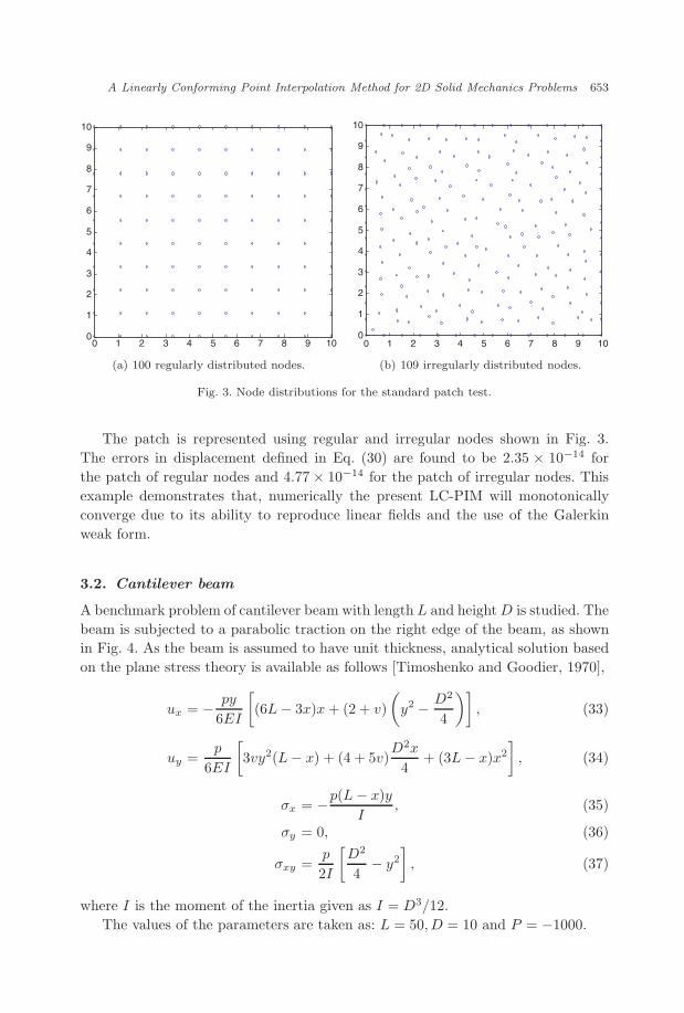
(a) 100 regularly distributed nodes. (b) 109 irregularly distributed nodes.

Fig. 3. Node distributions for the standard patch test.

The patch is represented using regular and irregular nodes shown in Fig. 3.The errors in displacement defined in Eq. (30) are found to be 2.35 × 10−14 forthe patch of regular nodes and 4.77 × 10−14 for the patch of irregular nodes. Thisexample demonstrates that, numerically the present LC-PIM will monotonicallyconverge due to its ability to reproduce linear fields and the use of the Galerkinweak form.

3.2. Cantilever beam

A benchmark problem of cantilever beam with length L and height D is studied. Thebeam is subjected to a parabolic traction on the right edge of the beam, as shownin Fig. 4. As the beam is assumed to have unit thickness, analytical solution basedon the plane stress theory is available as follows [Timoshenko and Goodier, 1970],

ux = − py

6EI

[(6L − 3x)x + (2 + v)

(y2 − D2

4

)], (33)

uy =p

6EI

[3vy2(L − x) + (4 + 5v)

D2x

4+ (3L − x)x2

], (34)

σx = −p(L − x)yI

, (35)

σy = 0, (36)

σxy =p

2I

[D2

4− y2

], (37)

where I is the moment of the inertia given as I = D3/12.The values of the parameters are taken as: L = 50, D = 10 and P = −1000.

March 2, 2006 11:32 WSPC/IJCM-j050 00066


L

x

y

D

P

Fig. 4. Cantilever beam subjected to a parabolic traction on the right edge.

Model-1

Model-2

Model-3

0 5 10 15 20 25 30 35 40 45 50-5

0

5

0 5 10 15 20 25 30 35 40 45 50-5

0

5

0 5 10 15 20 25 30 35 40 45 50-5

0

Fig. 5. Three models of nodal distributions for the cantilever beam.

3.2.1. Effects of the irregularity in the nodal distribution

To investigate the effect of the irregularities in nodal distribution, three modelsof 420 distributed nodes with different status of irregularity (shown in Fig. 5) areused to examine the present method. The results of deflection along the neutralline and the shear stress along the line (x = L/2) of the beam are plotted togetherwith the analytical solutions in Fig. 6. It can be found that the numerical results ofthese three models obtained using the present LC-PIM are all in good agreementwith the analytical ones, and the irregularity of the nodal distribution has littleeffect on the numerical results.

3.2.2. Convergence and efficiency of the LC-PIM

To investigate the properties of convergence and efficiency of the present method,four models with 94, 181, 399, and 801 irregularly distributed nodes are employed.

March 2, 2006 11:32 WSPC/IJCM-j050 00066


0 5 10 15 20 25 30 35 40 45 50-0.018

-0.016

-0.014

-0.012

-0.01

-0.008

-0.006

-0.004

-0.002

0

x

Def

lect

ion

Analytical solu.LC-PIM solu. (model-1)LC-PIM solu. (model-2)LC-PIM solu. (model-3)

-5 -4 -3 -2 -1 0 1 2 3 4 5-160

-140

-120

-100

-80

-60

-40

-20

0

y

She

ar s

tres

s

Analytical solu.LC-PIM solu. (model-1)LC-PIM solu. (model-2)LC-PIM solu. (model-3)

(a) Deflection distribution along the (b) Shear stress distribution along theneutral line. line x = L/2.

Fig. 6. Numerical results obtained using the LC-PIM and three models of node distributions.

10010-4

10-3

h

Err

or in

ene

rgy

FEM (R=1.0)RPIM (R=0.84)LC-PIM (R=1.42)

Fig. 7. Comparison of convergence rate between FEM, RPIM, and LC-PIM.

For comparison, three methods, FEM, RPIM, and LC-PIM, are all used forthis problem. In FEM, linear element of 3-node triangle is employed. In theRPIM, MQ-RBFs augmented with linear polynomials are adopted with parametersq = 1.03, αc = 4.0, and αs = 2.0 for circular local support domain. These valuesof parameters have been found to perform well for most problems [Wang and Liu,2002b; Liu, 2002; Liu et al., 2005]. The results of error in energy norm against h

are plotted in Fig. 7, where h is the averaged element size in the FEM. Comparedwith linear FEM, the LC-PIM not only achieves a higher convergence rate but alsoobtains more accurate results. This is due to the use of more nodes in creating theshape functions, which is made possible in the meshfree context, thus allowing theuse of nodes beyond the elements for shape function construction. Compared with

March 2, 2006 11:32 WSPC/IJCM-j050 00066


10010-4

10-3

CPU time

Err

or in

ene

rgy

FEMRPIMLC-PIM

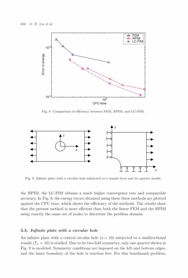
Fig. 8. Comparison of efficiency between FEM, RPIM, and LC-PIM.

x

y

x

y

Fig. 9. Infinite plate with a circular hole subjected to a tensile force and its quarter model.

the RPIM, the LC-PIM obtains a much higher convergence rate and comparableaccuracy. In Fig. 8, the energy errors obtained using these three methods are plottedagainst the CPU time, which shows the efficiency of the methods. The results showthat the present method is more efficient than both the linear FEM and the RPIMusing exactly the same set of nodes to discretize the problem domain.

3.3. Infinite plate with a circular hole

An infinite plate with a central circular hole (a = 10) subjected to a unidirectionaltensile (Tx = 10) is studied. Due to its two-fold symmetry, only one quarter shown inFig. 9 is modeled. Symmetry conditions are imposed on the left and bottom edges,and the inner boundary of the hole is traction free. For this benchmark problem,

March 2, 2006 11:32 WSPC/IJCM-j050 00066


the analytical solution is available [Timoshenko and Goodier, 1970]:

ur =Tx

4µ

r

[(κ − 1)

2+ cos(2θ)

]+

a2

r[1 + (1 + κ) cos(2θ)] − a4

r3cos(2θ)

, (38)

uθ =Tx

4µ

[(1 − κ)

a2

r− r − a4

r3

]sin(2θ), (39)

σxx = Tx

1 − a2

r2

[32

cos(2θ) + cos(4θ)]

+3a4

2r4cos(4θ)

, (40)

σyy = −Tx

a2

r2

[12

cos(2θ) − cos(4θ)]

+3a4

2r4cos(4θ)

, (41)

σxy = −Tx

a2

r2

[12

sin(2θ) + sin(4θ)]− 3a4

2r4sin(4θ)

, (42)

where

µ =E

2(1 + v), κ =

3 − 4v Plane strain3 − v

1 + vPlane stress

(43)

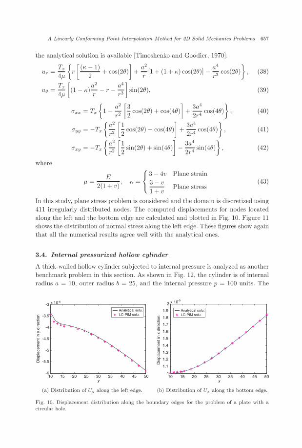
In this study, plane stress problem is considered and the domain is discretized using411 irregularly distributed nodes. The computed displacements for nodes locatedalong the left and the bottom edge are calculated and plotted in Fig. 10. Figure 11shows the distribution of normal stress along the left edge. These figures show againthat all the numerical results agree well with the analytical ones.

3.4. Internal pressurized hollow cylinder

A thick-walled hollow cylinder subjected to internal pressure is analyzed as anotherbenchmark problem in this section. As shown in Fig. 12, the cylinder is of internalradius a = 10, outer radius b = 25, and the internal pressure p = 100 units. The

10 15 20 25 30 35 40 45 50-6

-5.5

-5

-4.5

-4

-3.5

-3 x 10-6

Dis

plac

emen

t in

y di

rect

ion

y

Analytical solu.LC-PIM solu.

10 15 20 25 30 35 40 45 501

1.1

1.2

1.3

1.4

1.5

1.6

1.7

1.8

1.9

2 x 10-5

x

Dis

plac

emen

t in

x di

rect

ion


(a) Distribution of Uy along the left edge. (b) Distribution of Ux along the bottom edge.

Fig. 10. Displacement distribution along the boundary edges for the problem of a plate with acircular hole.

March 2, 2006 11:32 WSPC/IJCM-j050 00066


10 15 20 25 30 35 40 45 5010

12

14

16

18

20

22

24

26

28

30

y

σ xx


Fig. 11. Stress distribution along the left edge for the problem of a plate with a circular hole.

P

2015 15

y

x

Fig. 12. Hollow cylinder subjected to internal pressure and its quarter model.

thickness of the cylinder is of one unit and the analytical solution is available forthis plane stress problem [Timoshenko and Goodier, 1970].

ur =pa2

E(b2 − a2) r[(1 − v) r2 + (1 + v) b2], (44)

σr =a2p

b2 − a2

(1 − b2

r2

), (45)

σθ =a2p

b2 − a2

(1 +

b2

r2

). (46)

March 2, 2006 11:32 WSPC/IJCM-j050 00066


10 15 20 253

3.5

4

4.5

5

5.5

6 x 10-5

r

Dis

plac

emen

tAnalytical solu.LC-PIM solu.

Fig. 13. Displacement distribution along the left edge for the problem of internal pressurized hollowcylinder.

10 15 20 25−100

−50

0

50

100

150

r

stre

ss

Analytical solu. of σrAnalytical solu. of σθLC-PIM solu. of σrLC-PIM solu. of σ θ

Fig. 14. Stress distribution along the left edge for the problem of internal pressurized hollowcylinder.

In the study, the problem domain is represented with 441 irregularly distributednodes and the numerical solutions using LC-PIM are plotted in Figs. 13 and 14,together with the analytical solution. It can be observed that both the displacementand stress results are very accurate and stable, and in good agreement with theanalytical ones.

March 2, 2006 11:32 WSPC/IJCM-j050 00066


3.5. An automotive part: rim

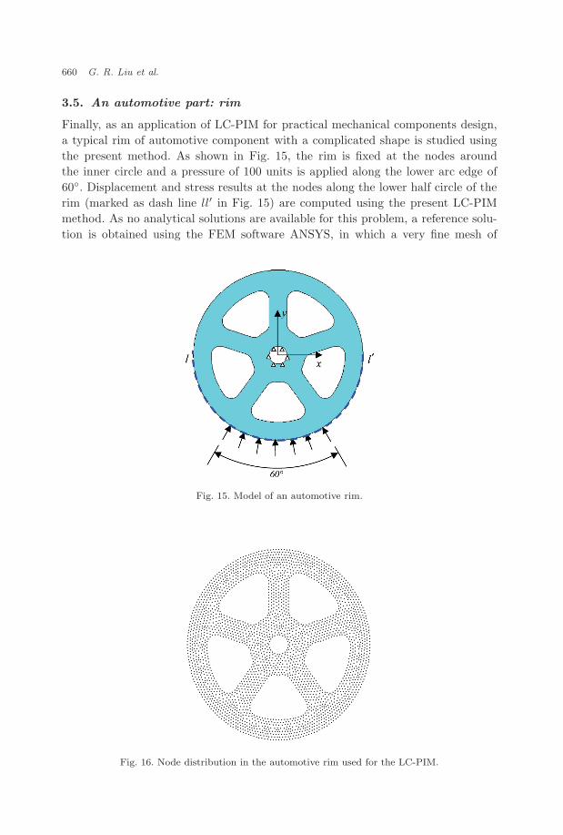
Finally, as an application of LC-PIM for practical mechanical components design,a typical rim of automotive component with a complicated shape is studied usingthe present method. As shown in Fig. 15, the rim is fixed at the nodes aroundthe inner circle and a pressure of 100 units is applied along the lower arc edge of60. Displacement and stress results at the nodes along the lower half circle of therim (marked as dash line ll′ in Fig. 15) are computed using the present LC-PIMmethod. As no analytical solutions are available for this problem, a reference solu-tion is obtained using the FEM software ANSYS, in which a very fine mesh of

Fig. 15. Model of an automotive rim.

Fig. 16. Node distribution in the automotive rim used for the LC-PIM.

March 2, 2006 11:32 WSPC/IJCM-j050 00066


6-node triangle element (18625 elements) is used. The problem domain is repre-sented with 2608 field nodes in our LC-PIM (shown in Fig. 16) and the numericalresults obtained using the present method are plotted in Figs. 17–21. It is foundthat both the computed displacements and stresses are in good agreement with thereference solutions.

-20 -15 -10 -5 0 5 10 15 20-1.5

-1

-0.5

0

0.5

1

1.5x 10-4

x

Dis

pla

cem

ent

in x

dire

ctio

n

Reference solu.LC-PIM solu.

Fig. 17. Distribution of Ux along the line ll′ on the boundary of the automotive rim.

-20 -15 -10 -5 0 5 10 15 200.5

1

1.5

2

2.5

3

3.5

4

4.5x 10-4

x

Dis

plac

emen

t in

y di

rect

ion


Fig. 18. Distribution of Uy along line ll′ on the boundary of the automotive rim.

March 2, 2006 11:32 WSPC/IJCM-j050 00066


-20 -15 -10 -5 0 5 10 15 20-600

-500

-400

-300

-200

-100

0

100

200

x

Nor

mal

str

ess

σ xx


Fig. 19. Distribution of σxx along the line ll′ on the boundary of the automotive rim.

-20 -15 -10 -5 0 5 10 15 20-150

-100

-50

0

50

100

x

Nor

mal

str

ess

σ yy


Fig. 20. Distribution of σyy along the line ll′ on the boundary of the automotive rim.

March 2, 2006 11:32 WSPC/IJCM-j050 00066


-20 -15 -10 -5 0 5 10 15 20-150

-100

-50

0

50

100

150

x

Shear

stre

ss σ

xy


Fig. 21. Distribution of σxy along the line ll′ on the boundary of the automotive rim.

4. Conclusions

In this work, a linearly conforming point interpolation method (LC-PIM) is pre-sented. The method employs polynomial basis functions for field approximation.Galerkin weak form is adopted, and a nodal integration scheme with strain smooth-ing operation is used. Numerical examples of standard patch test, three benchmarkproblems, and an actual application problem of a rim with complicated shape arestudied using the present LC-PIM method. Very accurate and stable results in termsof both displacements and stresses are obtained and compared with the analyticalor reference solutions. From the research, the following remarks can be made.

• Following the present scheme for local supporting nodes selection, the singu-larity problem of moment matrix in creating the PIM shape functions can besuccessfully resolved.

• The PIM shape functions generated posses many properties that are also foundin the conventional FEM (for example, the Kronecker delta function property)and most numerical techniques and treatments developed in FEM can be utilizedwith minor modifications.

• Nodal integration scheme with strain smoothing operation is adopted for thenumerical integration of the weak form. The present method so constructedguarantees a linear exactness of the numerical solutions, which was also provennumerically by the standard patch test.

• Compared with linear FEM of the linear triangle element, the LC-PIM usingexactly the same nodes distribution can achieve a better accuracy and higherconvergence rate.

March 2, 2006 11:32 WSPC/IJCM-j050 00066


• Compared with the original RPIM based on domain Gauss integration, thepresent LC-PIM needs no parameters, has higher convergence rate, compara-ble accuracy, and much better efficiency in the implementation.

As the present method successfully overcomes singularity problem of the momentmatrix, ensures linear conformability, and significantly improves the efficiency ofcomputing, the LC-PIM is expected to be further develop to deal with more com-plicated 3D problems with adaptive analysis capability.

References

Atluri, S. N. and Zhu, T. (1998). A new meshless local Petrov-Galerkin (MLPG) approachin computational mechanics. Comput. Mech. 22: 117–127.

Belytschko, T., Lu, Y. Y. and Gu, L. (1994). Element-free Galerkin methods. Int. J.Numer. Meth. Eng. 37: 229–256.

Chen, J. S., Wu, C. T., Yoon, S. and You, Y. (2001). A stabilized conformingnodal integration for Galerkin mesh-free methods. Int. J. Numer. Meth. Eng. 50:435–466.

Dai, K. Y., Liu, G. R., Han, X. and Li, Y. (2005). Inelastic analysis of 2D solids using ameshfree RPIM based on deformation theory. Computer Methods in Applied Mechanicsand Engineering (In press).

Liszka, T. and Orkisz, J. (1980). The finite difference methods at arbitrary irregular gridsand its applications in applied mechanics. Comput. & Struct. 11: 83–95.

Liu, G. R. (2002). Meshfree Methods: Moving Beyond the Finite Element Method. CRCPress, Boca Raton, USA.

Liu, G. R. and Gu, Y. T. (2001a). A point interpolation method for two-dimensional solids.Int. J. Numer. Meth. Eng. 50: 937–951.

Liu, G. R. and Gu, Y. T. (2001b). A local radial point interpolation method (LR-PIM)for free vibration analyses of 2-D solids. J. Sound Vib. 246(1): 29–46.

Liu, G. R. and Gu, Y. T. (2003). A matrix triangularization algorithm for point inter-polation method. Computer Methods in Applied Mechanics and Engineering 192(19):2269–2295.

Liu, G. R. and Gu, Y. T. (2005). An Introduction to Meshfree Methods and Their Pro-gramming. Springer, Dordrecht, The Netherlands.

Liu, G. R. and Liu, M. B. (2003). Smoothed Particle Hydrodynamics — A Meshfree Prac-tical Method. World Scientific, Singapore.

Liu, G. R., Zhang, G. R., Gu, Y. T. and Wang, Y. Y. (2005). A meshfree radial pointinterpolation method (RPIM) for three-dimensional solids. Computational Mechanics,36(6): 421–430.

Liu, W. K., Jun, S. and Zhang, Y. F. (1995). Reproducing kernel particle methods. Int.J. Numer. Methods Eng. 20: 1081–1106.

Lucy, L. (1977). A numerical approach to testing the fission hypothesis. Astron. J. 82:1013–1024.

Nayroles, B., Touzot, G. and Villon, P. (1992). Generalizing the finite element method:diffuse approximation and diffuse elements. Computational Mechanics 10: 307–318.

Timoshenko, S. P. and Goodier, J. N. (1970). Theory of Elasticity (3rd edition). McGraw-hill, New York.

Wang, J. G. and Liu, G. R. (2002a). A point interpolation meshless method based onradial basis functions. Int. J. Numer. Meth. Eng. 54: 1623–1648.

March 2, 2006 11:32 WSPC/IJCM-j050 00066


Wang, J. G. and Liu, G. R. (2002b). On the optimal shape parameters of radial basisfunctions used for 2-D meshless methods. Comput. Methods Appl. Mech. Eng. 191:2611–2630.

Wang, J. G., Liu, G. R. and Lin, P. (2002). Numerical analysis of Biot’s consolidationprocess by radial point interpolation method. Int. J. Solids Struct. 39(6): 1557–1573.

Zienkiewicz, O. C. and Taylor, R. L., The Finite Element Method. 5th edition. ButterworthHeinemann, Oxford, UK.

a linearly conforming point interpolation method (lc …

Documents