Consistent loosely coupled decentralized cooperative

navigation for team of mobile agents

Jianan Zhu Solmaz S. KiaUniversity of California Irvine

BIOGRAPHY

Jianan Zhu is a Ph.D. candidate in Mechanical and Aerospace Engineering Department at the

University of California, Irvine (UCI). He got his master’s degree in Mechanical and Aerospace

Engineering from UCI, Irvine and got his Bachelor’s degree in Tsinghua University, Beijing,

China. His research interest is in the distributed estimation algorithms in networked systems,

cooperative navigation of multiple mobile agents and its implementation, including consistent

decentralized cooperative navigation for mobile agents.

Solmaz Kia is an Assistant Professor in the Department of Mechanical and Aerospace Engineer-

ing, University of California, Irvine (UCI). She obtained her Ph.D. degree in Mechanical and

Aerospace Engineering from UCI, in 2009, and her M.Sc. and B.Sc. in Aerospace Engineering

from the Sharif University of Technology, Iran, in 2004 and 2001, respectively. She was a

senior research engineer at SySense Inc., El Segundo, CA from Jun. 2009-Sep. 2010. She held

postdoctoral positions in the Department of Mechanical and Aerospace Engineering at the UC

San Diego and UCI. She was the recipient of UC President’s Postdoctoral Fellowship from

2012-2014. Dr. Kia’s main research interests, in a broad sense, include distributed optimiza-

tion/coordination/estimation, nonlinear control theory and probabilistic robotics.

ABSTRACT

In this paper, a cooperative navigation algorithm for team of mobile agents is presented. The

proposed algorithm is a loosely coupled decentralized algorithm. The setting we consider consists

The authors are with the Department of Mechanical and Aerospace Engineering, University of California Irvine, Irvine,

CA 92697, USA, jiananz1@uci.edu,solmaz@uci.edu

Proceedings of the 2017 International Technical Meeting,ION ITM 2017, Monterey, California, January 30-February 2, 2017

782

of a set of mobile agents with sensing, processing and communication capabilities. In this setting

each agent maintains a local filter to propagate and update its local pose estimates using self-

motion measurements and occasional external absolute measurement signals. Whenever, an agent

takes a relative measurement with respect to a teammate, our proposed algorithm enables these

two agents to jointly process this relative measurements to update their local estimates in a

consistent manner in the absence of exact knowledge about the correlation between their local

estimates. Simulations demonstrate the benefits of our proposed algorithm.

I. INTRODUCTION

Determining the location of mobile agents (e.g, automobile, aerial vehicle, underwater vehicle,

ground robots) has always been a crucial factor for their autonomy in different circumstances,

either indoor or outdoor environments. Pose (position and orientation) information is essential in

other tasks such as path planning and environment monitoring. Navigation problem for mobile

agents consists of estimating the states of the agent using the sensor on board of the agent.

The basic idea here is to combine measurements from proprioceptive sensors that monitor the

motion of the vehicle with measurements from exteroceptive sensors that observe the surrounding

environment. The common navigation techniques rely on Global Positioning System (GPS) [1]

or use of external landmarks such as pre-installed beacons or fixed and stationary features in the

environment. In beacon-based localization [2] measurements taken from pre-installed markers

with known locations are used to improve the self-localization of mobile agents. The simultaneous

localization and map building (SLAM) techniques [3] use vision or LIDAR based measurements

from distinguishable features (landmarks) in the environment to build a map of the environment

and localize the agents in that map. These navigation techniques because of their reliance on

external services and features that may not necessarily be available in every environment do not

fully address the mobile agent localization problem.

An alternative navigation technique is cooperative navigation or cooperative localization ( as it is

more often referred too) [4]–[14]). In cooperative navigation, mobile agents, with communication

and computation capabilities, jointly process a relative measurement between each other (no

dependency on external features and services outside the team) to increase their localization

accuracy. Despite the great appeal of cooperative navigation for localization of team of networked

783

mobile agents in GPS and land-marked challenged environments, its integration in real world

applications has been challenging. Due to relative measurements updates, cooperative localiza-

tion results in strong couplings/cross correlations between the team members’ pose estimates.

Accounting for these coupling/cross correlations is crucial for filter consistency. It is well known

that disregarding the past correlations causes the so-called rumor propagation phenomenon that

can lead to overconfidence and, even to divergence of the estimates, as reported in [15]. However,

exact account of cross correlation terms comes with high computation and communication cost,

stringent requirement on network connectivity and communication channel utilization. In an

effort to develop practical cooperative localization algorithms, in this paper we propose a loosely

coupled algorithm where the correlations are accounted for in an implicit manner by conservative

but consistent estimate of joint covariance matrix of team members.

Related work: Under the assumption of Gaussian distribution for process and measurement

noises, [6] and [16] proposed a centralized Extended Kalman Filter (EKF) based cooperative

localization to propagate and update the estimates of all the agents in a jointly manner. Other

centralized cooperative localization algorithms to deal with non-Gaussian noises are discussed

in [12] and [13]. In a centralized cooperative localization algorithm, a fusion center (FC) which

is either a leader agent or a center overseeing the operation, is required. At each time step,

FC collects the individual motion measurements and agent-to-agent relative measurements to

estimate the team members poses or generate the update commands for the team members. Then,

the FC sends back this information to each agent In centralized operations the computation and

communication costs scale poorly with respect to the number of the agents in the team.

In recent years, to avoid single point failure and energy inefficiency of central operations,

many effort have been devoted to develop decentralized cooperative navigation algorithms. As

discussed in [14], the approaches to design decentralized cooperative localization algorithms can

be divided into two categories: tightly coupled algorithms and loosely coupled algorithms. In

tightly coupled approaches, normally the computations of a central cooperative localization is

distributed among the team members. Some examples of tightly coupled cooperative localization

algorithms can be found in ( [17], [18], [19], [13], [20]), where EKF based , Uncented Kalman

filter baed and maximum a posteriori based cooperative localization is decentralized among

team members. Tightly coupled algorithms, because of an accurate account of correlations

provide higher positioning accuracy but come with higher communication cost and stringent

784

network connectivity conditions. To avoid these costs, loosely coupled cooperative localization

methodologies, where the correlation terms are not maintained but accounted for in an implicit

way are proposed in the literature. In [21], an interleaved update algorithm was proposed to

provide consistent estimate that only the agent obtaining the relative measurement updates its

state. A bank of EKFs is maintained at each agent. Using an accurate bookkeeping of the

identity of the agents involved in previous updates and the age of such information, each of

these filters is only updated when its propagated state is not correlated to the state involved in

the current update equation. The main drawback is the growing size of information needed at

each update time which increases the computational complexity of the algorithm. Other loosely

couple cooperative localization algorithms mostly use covariance intersection method (c.f. [22],

[23]) in their approaches. Recall that the covariance intersection method fuses two or more tracks

from same process when the correlations between tracks are unknown. However, in cooperative

localization, the local pose estimates of two different mobile agents are jointly updated based on

the feedback from a relative measurement between them. As a result, cooperative localization

techniques which use covariance intersection method assume that each agent keeps a copy of the

state estimate of the entire team locally. See for example [15] which uses such an approach for

the localization of a group of space vehicles communicating over a fixed ring topology. Another

example of the use of split covariance intersection is given in [24] for intelligent transportation

vehicles localization. [25] uses a common past-invariant ensemble Kalman pose estimation filter

in another loosely-coupled CL approach for intelligent vehicles. This algorithm is very similar

to the decentralized covariance intersection data fusion method described above, with the main

difference that it operates with ensembles instead of with means and covariances. In a different

approach, to avoid the requirement for each agent to keep a copy of state estimate of the entire

team, [26] proposes an algorithm in which an agent taking relative pose measurement uses this

measurement and its current pose estimate to obtain and broadcast a pose and the associated

error covariance of its landmark agent (the landmark agent is the agent the relative measurement

is taken from). Then, the landmark agent uses the covariance intersection method to fuse the

newly acquired pose estimate with its own current estimate to increase its estimation accuracy.

This technique crucially relies on relative pose measurements and cannot be applied for the more

common cases of relative range and relative bearing measurements.

Contribution of the paper: In this paper, we develop a cooperative navigation method in which

785

correlations are not maintained explicitly but are accounted for in an implicit manner using

proper conservative but consistent estimate of the joint covariance of the agents. In our proposed

algorithm each agent maintains its local pose estimation algorithm which is propagated using self

motion-measurements and updated locally if occasional absolute measurements become available,

e.g., through occasional access to GPS signals. Whenever, an agent takes a relative measurement

from another agent in the team, this relative measurement is processed cooperatively by the two

agents involved using their current propagated state and covariance matrices. Our approach does

not require centralized data storage and processing. Moreover, it does not enforce a particular

communication hierarchy or topology and individual agents can join and leave the group without

the need to be aware of previous communications or the size of the group. Because, each agent

maintains its own local filter, our method is robust to communication failure. Finally, unlike

some other loosely coupled decentralized algorithms that only work for specific types of relative

measurement, our algorithm can process any form of relative measurement, i.e., there is no

restriction on the type of relative measurement for our algorithm. In short our main contribution

is a cooperative localization method that can be used as an add-on augmentation to improve self-

localization of the mobile agents. That is, agents can implement any localization strategy such

as dead-reckoning, GPS or SLAM and when the accuracy via these methods is not satisfactory,

they can seek assistance from other agents in their communication and relative measurement

device range without compromising the estimation consistency.

The outline of the paper is as follows: Section II describes our notations, terminologies and a

crucial lemma that we use to develop our results. Section III our loosely coupled decentralized

cooperative navigation algorithm’s derivation and its rigorous consistency analysis. We also

discuss two possible scenarios to implement our proposed algorithm. Section IV presents our

simulation studies.

II. PRELIMINARIES

This section described our notations, terminologies and a preliminary lemma we use in our

development in the proceeding sections.

Notations: the set of real and non-negative integer numbers are, respectively, R and Z++. The

set of n×n real positive definite matrices is S++n . The transpose of matrix A∈Rn×m is A>. For

786

a matrix A∈Rn×n, its trace is Tr(A) and its determinant is det(A). Considering a team of N

mobile agents, the local variables of agent i ∈ {1, · · · , N} are distinguished by the superscript

i, e.g., xi is the state (e.g., position and orientation) of agent i, xi is its state estimate, and Pi is

the covariance matrix of its state estimate, where xi, xi ∈ Rni and Pi ∈ S++ni . We use the term

cross-covariance to refer to the correlation terms between two agents in the joint covariance

matrix between them. We demonstrate the cross-covariance of the state vectors of agents i and

j by Pij ∈ Rni×nj . We denote the propagated and updated variables, say xi, at time-step k

by xi-(k) and xi+(k), respectively. We drop the time-step argument of the variables as well as

matrix dimensions whenever they are clear from the context. Next, we provide our definition of

estimator consistency which conforms with the definition given in [27].

Definition 1 (Consistency of an estimate): Given a process with state x, an state estimator

which produces estimate x with associated error covariance P is said to be consistent if it is

unbiased, i.e., E[x− x] = 0 and its state estimation error satisfies P ≥ E[(x− x)(x− x)>].

We should mention here that in some references the definition of estimator consistency includes

covariance matching condition P = E[(x− x)(x− x)>] (see e.g., [28], [29]).

In our developments below we use the following lemma.

Lemma 2.1 (A block diagonal upper bound on positive semi-definite matrices [30, page 207

and page 350]): Consider P1 ∈ S++n1

, P2 ∈ S++n2

and X ∈ Rn1×n2 such thatP1 X

X> P2

≥ 0.

Then, for any ω ∈ [0, 1], we have 1ωP1 0

0 11−ωP2

≥P1 X

X> P2

.

787

III. A LOOSELY COUPLED CONSISTENT COOPERATIVE LOCALIZATION

ALGORITHM

In this section we present our decentralized cooperative localization algorithm for a team of

mobile agents.

A. Description of the mobile agent team and problem setup

Consider a team of N collaborating mobile agents moving in a M-dimensional space. In this

team, each agent is capable of processing, measuring, and communicating. Each agent is equipped

with proprioceptive sensors (e.g., wheel encoders) that provide measurement of ego-motion, and

exteroceptive sensors (e.g., laser and vision) which enables the mobile agents to take relative

measurements from other team members. Also, each agent has a detectable unique identification

(UID), which here without loss of generality we assume to an integer i ∈ {1, · · · , N}. The

motion of each agent is modeled as a discrete-time time-varying linear system described by

xi(k + 1) = Fi(k)xi(k) + Bi(k)ui(k) + Gi(k)ηi(k), k ∈ Z++, (1)

where xi ∈ Rni , ui ∈ Rmi , and ηi ∈ Rpi are, respectively, the state, the control input and

the process noise of agent i. Here the process noise, ηi, i ∈ {1, · · · , N}, is an independent

zero-mean white Gaussian process with a known positive definite diagonal variance Qi(k) =

E[ηi(k)ηi(k)>] and uncorrelated in time. There is no requirement on the robotic team to be

homogeneous. Fi ∈ Rni×ni , Bi ∈ Rni×mi are the system matrices while Gi ∈ Rni×pi is the

coefficient matrix of process noise. It is also assumed that the process noise of each agent pair

i and j are mutually independent.

Every agent also carries exteroceptive sensors to detect, uniquely, the other agents in the team

and take relative measurements from them when they come to its limited measurement range.

The relative measurement collected by robot i from robot j is described by

zij(k) = Hiij(k)xi(k) + Hj

ij(k)xj(k) + νir(k), zij ∈ Rnirz , (2)

Every agent i ∈ {1, · · · , N} also has sensors on-board to collect absolute state measurement

when the opportunity to collect such measurement is present. We assume that such occasions

788

are limited. The absolute measurement model is as

zi(k) = Hi(k)xi(k) + νia(k), zi ∈ Rniaz , (3)

Hiij , Hj

ij and Hi are the measurement matrices of, respectively, relative and absolute mea-

surement. νir and νia are the respectively relative and absolute measurement noises of robot

i ∈ {1, · · · , N} that are both zero-mean white Gaussian processes with known diagonal co-

variance matrices Rir(k) and Ri

a(k). To be mentioned, all noises are assumed to be white and

mutually uncorrelated. Here, we assume that all the sensor measurements are synchronized.

For simplicity, in our aforementioned system model we used linear system model to describe

the mobile agents dynamics and measurement model. However, one may linearize a nonlinear

dynamics model about previous estimates to obtain the system matrices Fi, Bi, Gi, Hiij etc, for

all k ∈ Z++, see e.g. [19].

B. Consistent cooperative navigation under Unknown correlation

In a network of mobile agents deployed in a harsh environment, network connectivity is dynamic.

Communication failure due to obstacles and also agent’s limited communication is always

present. Additionally, mobile agents may join or leave the network, or may become unavailable

because of unpredictable failures or obstructions in the environment. All these considerations

make the design of effective tightly coupled cooperative localization algorithms challenging. To

address concerns about network connectivity, in the following, we propose a loosely coupled

cooperative localization algorithm in which we do not impose any connectivity condition for

the team. The setting in our algorithm is outline below: each agent i ∈ {1, · · · , N} maintains

its own local estimator to compute its pose estimate and the corresponding error covariance

without the need to communicate with other agents. When at any time k agent i takes a relative

measurement with respect to another agent j, it sends its local estimates and measurement

information to agent j. Agent j uses this information along its own local estimate to generate

a consistent update for both of the agents involved in the relative measurement. The updated

pose estimate for agent i then is sent back to that. In our setting, these two agents in the team

only need to communicate with each other when they want to process a relative measurement

between themselves (see Fig. 1). Normally communication range of mobile agents is larger than

789

Local

filterof

agent4

Local filter of agent 5

Loc

alfil

ter

ofag

ent

1

Local filter of agent 2Local filter of agent 3

Loos

ely

coup

led

coop

erat

ive

upda

te

Looselycoupled

cooperativeupdate

Relative measurement Exteroceptive sensing zone

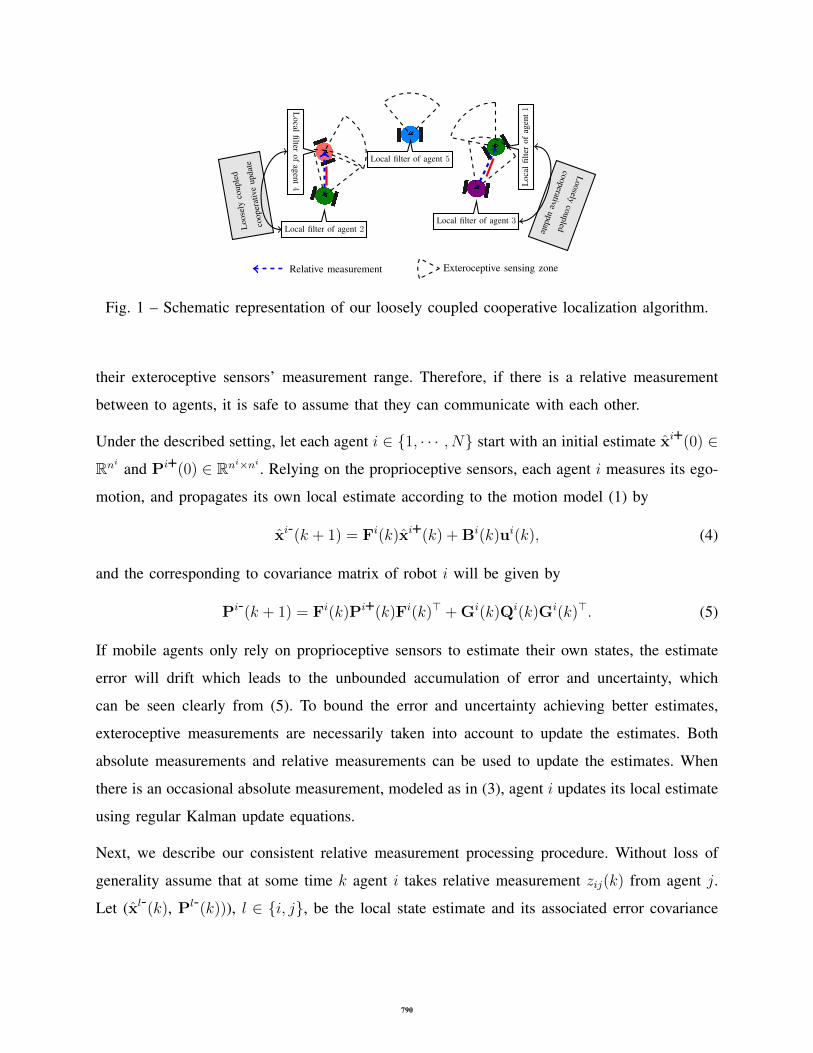
Fig. 1 – Schematic representation of our loosely coupled cooperative localization algorithm.

their exteroceptive sensors’ measurement range. Therefore, if there is a relative measurement

between to agents, it is safe to assume that they can communicate with each other.

Under the described setting, let each agent i ∈ {1, · · · , N} start with an initial estimate xi+(0) ∈

Rni and Pi+(0) ∈ Rni×ni . Relying on the proprioceptive sensors, each agent i measures its ego-

motion, and propagates its own local estimate according to the motion model (1) by

xi-(k + 1) = Fi(k)xi+(k) + Bi(k)ui(k), (4)

and the corresponding to covariance matrix of robot i will be given by

Pi-(k + 1) = Fi(k)Pi+(k)Fi(k)> + Gi(k)Qi(k)Gi(k)>. (5)

If mobile agents only rely on proprioceptive sensors to estimate their own states, the estimate

error will drift which leads to the unbounded accumulation of error and uncertainty, which

can be seen clearly from (5). To bound the error and uncertainty achieving better estimates,

exteroceptive measurements are necessarily taken into account to update the estimates. Both

absolute measurements and relative measurements can be used to update the estimates. When

there is an occasional absolute measurement, modeled as in (3), agent i updates its local estimate

using regular Kalman update equations.

Next, we describe our consistent relative measurement processing procedure. Without loss of

generality assume that at some time k agent i takes relative measurement zij(k) from agent j.

Let (xl-(k), Pl-(k))), l ∈ {i, j}, be the local state estimate and its associated error covariance

790

of agent l prior to updating them using relative measurement between them. The idea here is to

consider the states of agents i and j as joint state xJ , i.e.,

xJ(k) =

xj(k)

xj(k)

,with aggregated propagated/updated states prior to relative measurement processing as

x-J(k) =

xj-(k)

xj-(k)

.At time k, prior to the relative measurement update, the joint covariance matrix is P-

J (k)

P-J =

Pi-(k) P-ij(k)

P-ij>(k) Pj-(k)

. (6)

where the cross-covariance P-ij(k) is unknown. Our objective is to update x-

J(k) in a consistent

manner using the relative measurement (2). To account for the unknown cross-covariance matrix,

we invoke Lemma 2.1 to over-estimate the joint covariance by

P-J(k) =

1ωPi-(k) 0

0 11−ωP

j-(k)

≥ P-J(k), ∀ω ∈ [0, 1]. (7)

That is, in the update process the joint aggregated estimate is assume to be (x-J(k), P

-J(k)). The

states are updated according to

x+J (k) = x-

J(k) + Krij(k), (8)

where

rij(k) = zij(k)−Hiij(k)xi-(k)−Hj

ij(k)xj-(k).

For an optimal update we can use

K = argmin Tr(E[xJ(k)xJ(k)>]),

where xJ(k) = (xJ(k) − x+J (k)). However, because in the joint covariance matrix, the cross-

covariance term between the estimates of agents i and j is unknown, we use the over-estimated

joint covariance matrix PJ to obtain the Kalman gain from

K = argmin Tr((I−KH)P

-J(I−KH)> + KRi

rK>),

791

which obtains K such that an upper bound on Tr(E[xJ(k)xJ(k)>]) is minimized. Proceeding

with manipulation similar those used in the derivation of Kalman filter equations, we obtain the

Kalman gain and the corresponding covariance update as follows

K =

Ki

Kj

= P-JH>S−1ij

=

1ωPi-(k)Hi

ij>S−1ij

11−ωP

j-(k)Hjij>S−1ij

, (9)

and

P+J = (I−KH)P

-J(I−KH)> + KRi

rK>

= P-J −KSij K

>, (10)

where

Sij =HP-JH> + Ri

r(k)

=1

ωHiijP

i-(k)Hiij> +

1

1− ωHjijP

j-(k)Hjij> + Ri

r(k).(11)

Here, we used

H =[Hiij(k) Hj

ij(k)]. (12)

Next, we show that this over-estimation of the joint covariance matrix, results in consistent

updated estimates for agent i and j using relative measurements between them.

Theorem 3.1 (Consistency of the joint state estimate update using Kalman gain (9)): Let agent

i and agent j have unbiased and consistent estimates (xi-(k),Pi-(k)) and (xj-(k),Pj-(k)),

respectively, at time k. The updated joint estimate (x+J (k),P+

J (k)) where x+J and P+

J are

obtained from (8) and (10) with Kalman gain given in (9) is an unbiased and consistent estimate.

Proof- Given that the propagated joint estimate is unbiased (E[xJ(k) − x-J(k)] = 0.), and the

measurement noise is zero mean, the joint updated state is unbiased, i.e., E[xJ(k)− x+J (k)] = 0.

To prove consistency in the sense we defined in Definition 1, we need to show that

P+J ≥ E[xJ(k)xJ(k)>],

792

where xJ(k) = (xJ(k)− x+J (k)). To this end, recall that

P+J = (I−KH)P

-J(I−KH)> + KRi

rK>

and

E[xJ(k)xJ(k)>]=(I−KH)P-J(I−KH)> + KRi

rK>,

where P-J is the joint covariance matrix between estimates of agent i and j as described in (6)

with unknown cross-covariance matrix. Then,

P+J − E[xJ(k)xJ(k)>]=(I−KH)(P

-J −P-

J)(I−KH)>,

which given (7), guarantees P+J −E[xJ(k)xJ(k)>] ≥ 0, and thus, the consistency of the updated

estimate. �

Theorem 3.1 showed that for any ω ∈ [0, 1] updating the state estimates of agents i and j using

the gain (9) results in a consistent estimate. Next, to achieve the maximum benefit in reducing

the joint uncertainty we obtain an optimal ω? ∈ [0, 1] from

ω? = argmaxω∈[0,1]

det(P+J

−1), (13)

which can be cast in an equivalent convex optimization problem form

ω? = argminω∈[0,1]

− log det(P+J

−1)

= argminω∈[0,1]

− log det(P-J−1 + H>Ri

r

−1H), (14)

that is

ω? = argminω∈[0,1]

− log det(

ωPi-−1 0

0 (1− ω)Pj-−1

+ H>Rir

−1H).

Here, we used

P+J = P

-J −KS−1ij K

>

= P-J − P

-JH>(HP

-JH> + Ri

r)−1HP

-J ,

and matrix inversion Lemma to write

P+J

−1= P

-J−1 + H>Ri

r

−1H.

793

We used det(P+J ) as our measure of total uncertainty. Alternatively, we can use Tr(P+

J ) as the

measure of total uncertainty and obtain ω? from minimizing the trace uncertainty measure.

Remark 3.1 (Uncertainty reduction in the loosely coupled cooperative localization algorithm):

The prior covariance matrix of each robot is Pi- and Pj-. The joint covariance after the update

is given by (10) whose elements for each agent read as follows (recall Sij in (11))

Pi+ =1

ω?Pi- −KiSijKi

> (15a)

=1

ω?Pi- − (

1

ω?)2Pi-Hi

ij>S−1ij H

iijP

i-,

Pj+ =1

1− ω?Pj- −KjSijKj

> (15b)

=1

1− ω?Pj-− (

1

1− ω?)2Pj-Hj

ij

>S−1ij H

jijP

j-,

where recall that ω? ∈ [0, 1] and as a result we have 1ω? ≥ 0 and 1

1−ω? ≥ 1. In the update

procedure to preserve filter consistency in the presence of unknown prior cross covariance, we

first over estimate the covariance. Then the uncertainty is reduced from this enlarged uncertainty

by using the relative measurement processing as we can see in (15). Using the determinant of

the local updated covariance as our measure of uncertainty of each agent, we can use ga(ω?),

a ∈ {i, j}, defined as follows, as a measure to devalue the reduction in the uncertainty of the

agents (recall (15))

det(Pi+) = gi(ω) det(Pi-), det(Pj+) = gj(ω) det(Pj-), (16)

where

gi(ω) = det( 1

ωI− (

1

ω)2√Pi->Hi

ij>S−1ij H

iij

√Pi-),

gj(ω) = det( 1

1−ωI−(

1

1−ω)2√Pj->Hj

ij>S−1ij H

jij

√Pj-).

�

The experiment depicted in Fig. IV demonstrates the reduction in the uncertainty of the mobile

agents after implementing our proposed loosely coupled algorithm for cooperative localization

(the blue circles highlight the onset of implementing our propose algorithms)–for details of this

numerical experiment please see Section IV.

794

In the following, we discuss an alternative approach to design the optimal ω in a manner that we

can place weight on which agent to receive more improvement from the cooperative localization

update. We use, once again, the determinant of the local updated covariance as our measure of

uncertainty of each agent. Remark that applying the matrix inversion Lemma on (15), we can

obtain the inverse of the local updated covariance matrices as follows

Pi+−1 =ωPi-−1 + (1− ω)Hiij

>(Hj

ijPj-Hj

ij> + (1− ω)Ri

r)−1Hi

ij, (17a)

Pj+−1 =(1− ω)Pj-−1 + ωHjij

>(Hi

ijPi-Hi

ij

>+ ωRi

r)−1Hj

ij. (17b)

We define our alternative weighted objective function to obtain ω? as

ω? = argmaxω∈[0,1]

ci log det(Pi+−1) + cj log det(Pj+−1). (18)

Here, ci ≥ 0 and cj ≥ 0 are the weights which are introduced to adjust the gain each agent can

achieve from the cooperative localization update. An interesting scenario that can be constructed

from this optimization routine is when we allow one of the agents, say without loss of generality

agent i, to act selfishly. That is, we let cj = 0. This scenario would be of interest in cases that

one of the team members is likely to have more accurate positioning estimates than the other

teammate. For example in underwater operations around a surface mother-ship, the mother-ship

because of its access to GPS, will have more accurate positioning than the underwater vehicles.

Remark 3.2 (Extension to local filters other than Kalman filter): In our algorithm, the coopera-

tive relative measurement processing problem with unknown cross-covariance is changed into the

joint update of (xi-, 1wPi-) and (xj-, 1

1−wPj-) using the relative measurement, with no correlation

between these estimates. Therefore, the local filters and the filter used to update the estimates

is not restricted to be a Kalman filter and other estimation filters such as UKF can also be used

to process the relative measurement. �

C. Consistent loosely coupled cooperative navigation algorithms

Using the theoretical developments in Section III-B, we propose two consistent loosely coupled

cooperative navigation algorithms as described in Algorithm 1 and Algorithm 2. In Algorithm 1,

which we refer to it as ‘Mutualistic1 Cooperative Localization’, agents engaged in a relative

1In biology muturalism is a symbiotic relation that both organisms benefit from their cooperation.

795

measurement minimize their joint total uncertainty by implementing ω? obtained from (14).

Moreover, both agents update their estimates, in a consistent manner, using the relative mea-

surement between them. In Algorithm 2, which we refer to it as ‘Commensalistic2 Cooperative

Localization’, to obtain the update gain, one of the agents selfishly minimizing its own local

updated covariance matrix with respect to ω (i.e., the selfish agent sets the weight of the other

agent in (18) equal to zero). In our algorithms presentation here, for brevity, we only discuss the

case where at each time each agent is only engaged in one relative measurement. We also do

not discuss the details of processing absolute measurements. These case can be processed using

sequential processing procedure (consult, for example, [31, Ch. 3], [32]). Details are omitted for

brevity.

For any agent a ∈ {1, · · · , N}, we let Vacoop(k) ⊆ {1, · · · , N} be the set of agents that agent

a ∈ {1, · · · , N} prior to the current time k has updated its estimates by cooperating with them

plus the agent a itself. Two observation are in order here. One is that the state estimate of agent

a at time k is correlated with the state estimate of agents in Vacoop(k). Also, at any time k, for

any agent b ∈ Vacoop(k), the state estimate of agent a is correlated with the state estimate of all

the agents in Vbcoop(k). In our algorithms described below, we do not keep an accurate account

of these correlations but account for them in an implicit manner using the method we developed

in Section III-B.

IV. NUMERICAL SIMULATIONS

We test the performance of our proposed loosely coupled consistent cooperative localization

algorithms (Mutualistic Cooperative Localization and Coomensalistic Cooperative Localization)

in simulations for a group of 3 robots moving on a flat terrain. The simulations are run for

1000 time steps (each time step has a duration of 0.1 sec). Each robot measures its linear,

ν, and angular velocity, ω, with independent zero-mean white Gaussian noises with standard

deviation σν = 0.1m/s and σω = 2 deg/s. The relative measurements used in the simulation are

relative range and relative bearing. We set the measurement noise to be independent zero-mean

white Gaussian distributed with standard deviation σr = 0.05m and σφ = 1 deg. Each robot

propagates its own state at every time step while the measurement update happens when relative

2In biology commensalism is a symbiotic relation that one of the organisms benefit and the other is unaffected

796

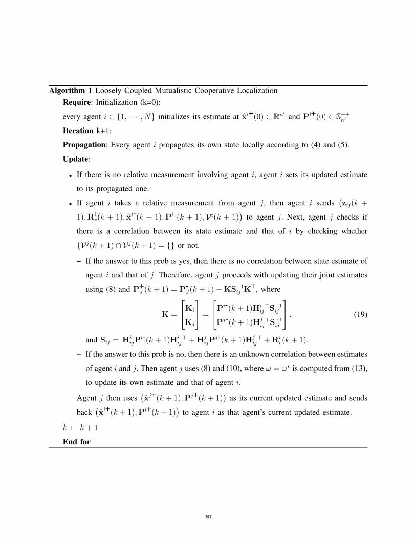
Algorithm 1 Loosely Coupled Mutualistic Cooperative LocalizationRequire: Initialization (k=0):

every agent i ∈ {1, · · · , N} initializes its estimate at xi+(0) ∈ Rni and Pi+(0) ∈ S++ni

Iteration k+1:

Propagation: Every agent i propagates its own state locally according to (4) and (5).

Update:

• If there is no relative measurement involving agent i, agent i sets its updated estimate

to its propagated one.

• If agent i takes a relative measurement from agent j, then agent i sends(zij(k +

1),Rir(k + 1), xi-(k + 1),Pi-(k + 1),V i(k + 1)

)to agent j. Next, agent j checks if

there is a correlation between its state estimate and that of i by checking whether

{Vj(k + 1) ∩ Vj(k + 1) = {} or not.

– If the answer to this prob is yes, then there is no correlation between state estimate of

agent i and that of j. Therefore, agent j proceeds with updating their joint estimates

using (8) and P+J (k + 1) = P-

J(k + 1)−KS−1ij K>, where

K =

Ki

Kj

=

Pi-(k + 1)Hiij>S−1ij

Pj-(k + 1)Hjij>S−1ij

, (19)

and Sij = HiijP

i-(k + 1)Hiij> + Hj

ijPj-(k + 1)Hj

ij> + Ri

r(k + 1).

– If the answer to this prob is no, then there is an unknown correlation between estimates

of agent i and j. Then agent j uses (8) and (10), where ω = ω? is computed from (13),

to update its own estimate and that of agent i.

Agent j then uses(xj+(k + 1),Pj+(k + 1)

)as its current updated estimate and sends

back(xi+(k + 1),Pi+(k + 1)

)to agent i as that agent’s current updated estimate.

k ← k + 1

End for

797

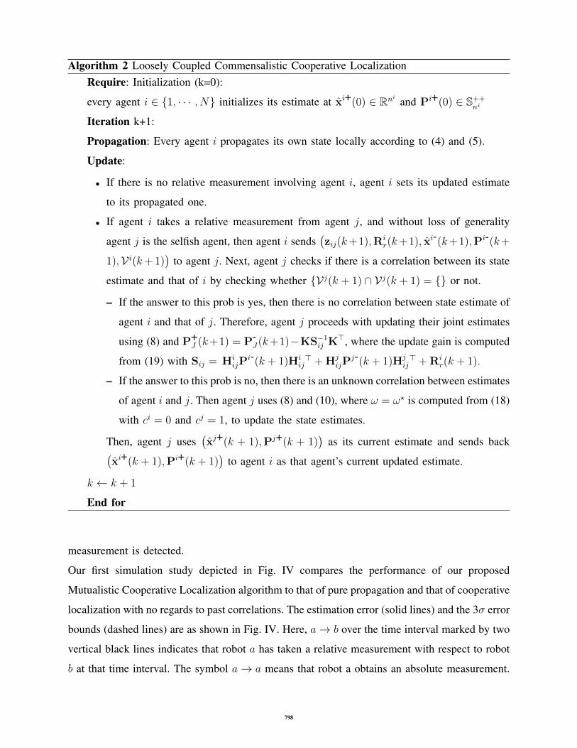
Algorithm 2 Loosely Coupled Commensalistic Cooperative LocalizationRequire: Initialization (k=0):

every agent i ∈ {1, · · · , N} initializes its estimate at xi+(0) ∈ Rni and Pi+(0) ∈ S++ni

Iteration k+1:

Propagation: Every agent i propagates its own state locally according to (4) and (5).

Update:

• If there is no relative measurement involving agent i, agent i sets its updated estimate

to its propagated one.

• If agent i takes a relative measurement from agent j, and without loss of generality

agent j is the selfish agent, then agent i sends(zij(k+1),Ri

r(k+1), xi-(k+1),Pi-(k+

1),V i(k+ 1))

to agent j. Next, agent j checks if there is a correlation between its state

estimate and that of i by checking whether {Vj(k + 1) ∩ Vj(k + 1) = {} or not.

– If the answer to this prob is yes, then there is no correlation between state estimate of

agent i and that of j. Therefore, agent j proceeds with updating their joint estimates

using (8) and P+J (k+1) = P-

J(k+1)−KS−1ij K>, where the update gain is computed

from (19) with Sij = HiijP

i-(k + 1)Hiij> + Hj

ijPj-(k + 1)Hj

ij> + Ri

r(k + 1).

– If the answer to this prob is no, then there is an unknown correlation between estimates

of agent i and j. Then agent j uses (8) and (10), where ω = ω? is computed from (18)

with ci = 0 and cj = 1, to update the state estimates.

Then, agent j uses(xj+(k + 1),Pj+(k + 1)

)as its current estimate and sends back(

xi+(k + 1),Pi+(k + 1))

to agent i as that agent’s current updated estimate.

k ← k + 1

End for

measurement is detected.

Our first simulation study depicted in Fig. IV compares the performance of our proposed

Mutualistic Cooperative Localization algorithm to that of pure propagation and that of cooperative

localization with no regards to past correlations. The estimation error (solid lines) and the 3σ error

bounds (dashed lines) are as shown in Fig. IV. Here, a→ b over the time interval marked by two

vertical black lines indicates that robot a has taken a relative measurement with respect to robot

b at that time interval. The symbol a→ a means that robot a obtains an absolute measurement.

798

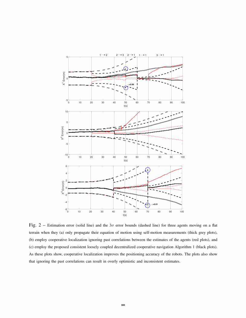
At the time step t = 20s, agent 1 take relative measurement from agent 2 for the first time. As

there is no correlation yet between agent 1 and agent 2, independence holds here at this instant.

Afterwards, the correlation between agent 1 and 2 is established and it should be taken into

account. At the time step t = 40s, similarly, agent 2 takes its first relative measurement from

agent 3. Once again as there is no correlation between these two robots’ estimates, independence

holds. Afterwards, the correlation should be taken into account. As Fig. IV shows, ignoring the

past correlations leads to inconsistent estimates (see red plots). Recall that the correlation is not

only established by direct relative measurement update between two robots but also by indirect

manner as well. For example, at time t = 70s, agent 3 takes a relative measurement from agent 1

for the first time. But at this point, their estimates are correlated because of both simultaneously

being correlated with robot 2. As shown, the proposed method without keeping track of the

cross-covariances is consistent and has a significant reduction of uncertainty compared to the

pure propagation case. As we can see from t = 60s to t = 70s, as agent 1 takes benefit from

the absolute measurements, it pose accuracy improves significantly. When agent 3 takes relative

measurement from agent 1 afterwards, the high accuracy of agent 1 also benefits agent 3. Next,

the root mean square error (RMSE) criterion was employed to test the accuracy (averaged over

50 Monte Carlo runs) as shown in Fig. 3. A reduction of RMSE can be observed for the proposed

method.

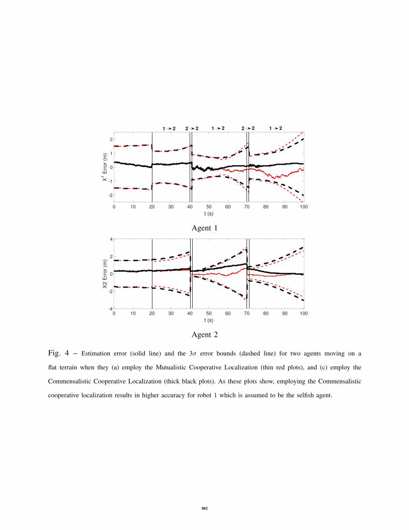
Our second simulation study depicted in Fig. 4 compares the performance of our proposed

Mutualistic Cooperative Localization algorithm (thin red plots) and the Commensalistic Cooper-

ative Localization (thick black plots) for two robots. Here, we assume that robot 1 needs higher

accuracy in its positioning therefore in the Commensalistic Cooperative Localization algorithm

we let this agent to be the selfish agent, i.e., at the time of relative measurement processing we

set c1 = 1 and c2 = 0 in (18). As Fig. 4 shows in the Commensalistic Cooperative Localiza-

tion algorithm, agent 1 acquires higher precision than in Mutualistic Cooperative Localization

algorithm.

799

0 10 20 30 40 50 60 70 80 90 100

t(s)

-5

0

5

X1 E

rror(

m)

1 2 12 3 2 1 1 3 1

ω=0.89

0 10 20 30 40 50 60 70 80 90 100

t(s)

-10

-5

0

5

10

X2 E

rror(

m)

0 10 20 30 40 50 60 70 80 90 100

t(s)

-6

-4

-2

0

2

4

6

X3 E

rror(

m)

ω=0.01

Fig. 2 – Estimation error (solid line) and the 3σ error bounds (dashed line) for three agents moving on a flat

terrain when they (a) only propagate their equation of motion using self-motion measurements (thick grey plots),

(b) employ cooperative localization ignoring past correlations between the estimates of the agents (red plots), and

(c) employ the proposed consistent loosely coupled decentralized cooperative navigation Algorithm 1 (black plots).

As these plots show, cooperative localization improves the positioning accuracy of the robots. The plots also show

that ignoring the past correlations can result in overly optimistic and inconsistent estimates.

800

0 10 20 30 40 50 60 70 80 90 100

time(s)

0

1

2

3

4

5

Positio

n R

MS

E(m

)

Fig. 3 – The root mean square error (RMSE) of the agents for the simulation averaged over 50 Monte Carlo runs

and over all agents. The agents (a) only propagate their equation of motion using self-motion measurements (thick

grey plots), (b) employ cooperative localization ignoring past correlations between the estimates of the agents (red

plots), and (c) employ the proposed consistent loosely coupled decentralized cooperative navigation Algorithm 1

(black plots). As seen, cooperative localization via Algorithm 1 results in improving the position accuracy of the

robots which cooperative localization ignoring past correlations results in eventually highly inaccurate positioning

results, to the point that is is not seen in the window shown.

801

0 10 20 30 40 50 60 70 80 90 100

t (s)

-2

-1

0

1

2

X1 E

rror

(m)

1 2 2 1 222221

Agent 1

0 10 20 30 40 50 60 70 80 90 100

t (s)

-4

-2

0

2

4

X2

Err

or

(m)

Agent 2

Fig. 4 – Estimation error (solid line) and the 3σ error bounds (dashed line) for two agents moving on a

flat terrain when they (a) employ the Mutualistic Cooperative Localization (thin red plots), and (c) employ the

Commensalistic Cooperative Localization (thick black plots). As these plots show, employing the Commensalistic

cooperative localization results in higher accuracy for robot 1 which is assumed to be the selfish agent.

802

References

[1] S. Cooper and H. Durrant-Whyte, “A Kalman filter model for GPS navigation of land vehicles,” in IEEE/RSJ Int. Conf.

on Intelligent Robots & Systems, (Munich, Germany), pp. 157–163, 1994.

[2] J. Leonard and H. F. Durrant-Whyte, “Mobile robot localization by tracking geometric beacons,” IEEE Transactions on

Robotics and Automation, vol. 7, pp. 376–382, June 1991.

[3] G. Dissanayake, P. Newman, H. F. Durrant-Whyte, , S. Clark, and M. Csorba, “A solution to the simultaneous localization

and map building (SLAM) problem,” IEEE Transactions on Robotics and Automation, vol. 17, no. 3, pp. 229–241, 2001.

[4] R. Kurazume, S. Nagata, and S. Hirose, “Cooperative positioning with multiple robots,” in IEEE Int. Conf. on Robotics

and Automation, pp. 1250–1257, 1994.

[5] I. Rekleitis, G. Dudek, and E. Milios, “Multi-robot collaboration for robust exploration,” in IEEE Int. Conf. on Robotics

and Automation, pp. 3164–3169, 2000.

[6] S. I. Roumeliotis, Robust mobile robot localization: from single-robot uncertainties to multi-robot interdependencies. PhD

thesis, University of Southern California, 2000.

[7] A. Howard, M. Matark, and G. Sukhatme, “Localization for mobile robot teams using maximum likelihood estimation,”

in IEEE/RSJ Int. Conf. on Intelligent Robots & Systems, vol. 1, pp. 434–439, 2002.

[8] E. D. Nerurkar, S. I. Roumeliotis, and A. Martinelli, “Distributed maximum a posteriori estimation for multi-robot

cooperative localization,” in IEEE Int. Conf. on Robotics and Automation, (Kobe, Japan), pp. 1402–1409, May 2009.

[9] D. Fox, W. Burgard, H. Kruppa, and S. Thrun, “A probabilistic approach to collaborative multi-robot localization,”

Autonomous Robots, vol. 8, no. 3, pp. 325–344, 2000.

[10] A. Howard, M. J. Mataric, and G. S. Sukhatm, “Putting the ‘I’ in ‘team’: An ego-centric approach to cooperative

localization,” in IEEE Int. Conf. on Robotics and Automation, vol. 1, pp. 868–874, 2003.

[11] A. Prorok and A. Martinoli, “A reciprocal sampling algorithm for lightweight distributed multi-robot localization,” in

IEEE/RSJ Int. Conf. on Intelligent Robots & Systems, pp. 3241–3247, 2011.

[12] A. T. Ihler, J. W. Fisher, R. L. Moses, and A. S. Willsky, “Nonparametric belief propagation for self-localization of sensor

networks,” IEEE Journal of Selected Areas in Communications, vol. 23, no. 4, pp. 809–819, 2005.

[13] J. Nilsson, D. Zachariah, I. Skog, and P. Handel, “Cooperative localization by dual foot-mounted inertial sensors and

inter-agent ranging,” EURASIP Journal on Advances in Signal Processing, vol. 2013, no. 164, 2013.

[14] S. S. Kia, S. Rounds, and S. Martınez, “Cooperative localization for mobile agents: a recursive decentralized algorithm

based on Kalman filter decoupling,” IEEE Control Systems Magazine, vol. 36, no. 2, pp. 86–101, 2016.

[15] P. O. Arambel, C. Rago, and R. K. Mehra, “Covariance intersection algorithm for distributed spacecraft state estimation,”

in American Control Conference, (Arlington, VA), pp. 4398–4403, 2001.

[16] S. I. Roumeliotis and G. A. Bekey, “Distributed multirobot localization,” IEEE Transactions on Robotics and Automation,

vol. 18, no. 5, pp. 781–795, 2002.

[17] N. Trawny, S. I. Roumeliotis, and G. B. Giannakis, “Cooperative multi-robot localization under communication constraints,”

in IEEE Int. Conf. on Robotics and Automation, (Kobe, Japan), pp. 4394–4400, May 2009.

[18] K. Y. K. Leung, T. D. Barfoot, and H. H. T. Liu, “Decentralized localization of sparsely-communicating robot networks:

A centralized-equivalent approach,” IEEE Transactions on Robotics, vol. 26, no. 1, pp. 62–77, 2010.

[19] S. S. Kia, S. Rounds, and S. Martınez, “A centralized-equivalent decentralized implementation of extended Kalman filters

for cooperative localization,” in IEEE/RSJ Int. Conf. on Intelligent Robots & Systems, (Chicago, IL), pp. 3761–3765,

September 2014.

803

[20] V. Dinh and S. S. Kia, “A server-client based distributed processing for an unscented Kalman filter for cooperative

localization,” in International Conference on Multisensor Fusion and Integration for Intelligent Systems, (San Diego, CA),

pp. 43–48, 2015.

[21] A. Bahr, M. R. Walter, and J. J. Leonard, “Consistent cooperative localization,” in IEEE Int. Conf. on Robotics and

Automation, (Kobe, Japan), pp. 8908–8913, May 2009.

[22] S. J. Julier and J. K. Uhlmann, “A non-divergent estimation algorithm in the presence of unknown correlations,” in American

Control Conference, vol. 4, pp. 2369–2373, Jun 1997.

[23] S. J. Julier and J. K. Uhlmann, Handbook of Data Fusion. CRC Press, 2001.

[24] H. Li and F. Nashashibi, “Cooperative multi-vehicle localization using split covariance intersection filter,” vol. 5, no. 2,

pp. 33–44, 2013.

[25] D. Marinescu, N. O’Hara, and V. Cahill, “Data incest in cooperative localisation with the common past-invariant ensemble

kalman filter,” in IEEE Int. Conf. on Information Fusion, (Istanbul, Turkey), pp. 68–76, 2013.

[26] L. C. Carrillo-Arce, E. D. Nerurkar, J. L. Gordillo, and S. I. Roumeliotis, “Decentralized multi-robot cooperative localization

using covariance intersection,” in IEEE/RSJ Int. Conf. on Intelligent Robots & Systems, (Tokyo, Japan), pp. 1412–1417,

2013.

[27] S. J. Julier and J. K. Uhlmann, “A non-divergent estimation algorithm in the presence of unknown correlations,” in American

Control Conference, pp. 2369–2373, 1997.

[28] H. Durrant-Whyte, “Introduction to estimation and the Kalman filter,” University of Sydney, Australian Centre for Field

Robotics, 2001.

[29] Y. Bar-Shalom, X. R. Li, and T. Kirubarajan, Estimation with Applications to Tracking and Navigation. John Wiley, 2001.

[30] R. A. Horn and C. R. Johnson, Topics in Matrix Analysis. Cambridge: Cambridge University Press, 1991.

[31] C. T. Leondes, ed., Advances in Control Systems Theory and Application, vol. 3. New York: Academic Press, 1966.

[32] Y. Bar-Shalom, P. K. Willett, and X. Tian, Tracking and Data Fusion, a Handbook of Algorithms. Storts, CT, USA: YBS

Publishing, 2011.

804