a low-cost, wireless, multi-modal sensing network for...
TRANSCRIPT

1
A Low-Cost, Wireless, Multi-Modal SensingNetwork for Driving Behavior Modeling and Early
Collision WarningHamad Ahmed, Member, IEEE, and Muhammad Tahir, Member, IEEE
Abstract—Traffic accidents have escalated to an alarming levelin the last decade or so, mainly due to inattentive and rashdriving behavior. Recent research efforts have resulted in systemsfor automatic detection of abnormal driving, that can warn thedriver as well as notify traffic authority so that the personcan be taken off the roads. However, these systems lack large-scale deployment as they are expensive and suffer from falsepositives. Driving is a complex multi-dimensional interactionof the driver with his environment. Therefore, to effectivelycapture the driving behavior, information of surrounding vehiclesshould be considered as well, which is also missing in existingsystems. In this paper, we have proposed a multi-modal vehicularsensor network which is low-cost and uses both the vehicle’smotion profile and surrounding traffic information for behaviormodeling. Heading (pose) and speed of the vehicle are determinedfrom an IMU and vehicle CAN bus respectively, whereas thesurrounding traffic is sensed and tracked by a LIDAR. To processand fuse the data of various sensors, algorithms of low-complexityare proposed which are able to run on low-cost microprocessors,thus removing the need of an on-vehicle computer which furtherreduces the cost of the system. We also provide early warnings ofrisk of collisions based on the motion of surrounding traffic andthe driver’s intent inferred from his eye movements which aretracked by a camera. The hardware architecture of the systemis also discussed. Experimental results on a test vehicle in realtraffic scenario show robustness to false positives.
Index Terms—Driver Safety, Driving Behavior, Driving Events,Aggressive Driving, IMU, Kalman Filter.
I. INTRODUCTION
STEADY development of motor vehicles during the 20thcentury has greatly influenced human life, providing
greater mobility for people and promoting socio-economicdevelopment. However the alarming increase in traffic con-gestion has not been matched with adequate availability ofsafety measures, making motor vehicle accidents a majorcause of death. According to National Highway Traffic SafetyAdministration (NHTSA), 32,675 people died in U.S. due toroad accidents in 2014. Roughly one-third deaths occurreddue to drunk driving and an additional 12.5% occurred dueto inattentive driving [1]. Furthermore, the first six monthsof 2015 have already seen an alarming increase of 8.1% inthis fatality rate as compared to 2014. In order to address thisstartling situation and increase road safety, several methodshave been used over the years including traffic monitoringcameras and strict penalties on breaking traffic laws. Thesehave somewhat forced the drivers to drive within safety limitsbut the fatality rate still continues to rise. There is a needto catch drunk drivers, alert inattentive drivers and force rashdrivers to drive safely.
It has been shown that drivers tend to drive attentively andare unlikely to perform rash maneuvers when they know thatthey are being monitored [2]. For example, drivers are lesslikely to take a red light when they know that cameras arewatching as compared to when there are no cameras. ‘Howam I driving’ bumper stickers and call service are utilizedfor this same purpose. These stickers are installed on trucks,buses and other commercial vehicles and the companies claimthat drivers are less likely to engage in unsafe maneuvers whenthey are being monitored due to these stickers [3]. However aspointed out in [4], it is not practical for someone to actuallycall the hotline and complain about somemone’s driving asusing cell phones are not allowed while driving and 76% ofworkers drive alone to work which means that there is nopassenger available to make the call.
To overcome these issues, researchers have developed sys-tems that can be installed on vehicles to automatically monitordriving behavior. These systems serve to alert a driver ifthey sense inattentive driving or provide feedback to thedriver in case of rash driving. The functionality can also beextended to notify traffic authorities if the driver continuesrash driving or in case of drunk driving. With the help ofcertain sensors, speed and heading (pose) of the car aredetermined and modeling or learning based techniques areapplied to determine ‘Driving Events’ or maneuvers. Theseevents include accelerating, decelerating, lane changes andturns. Based on the nature and frequency of these drivingevents, driving behavior of the driver is determined.
The measure of success of such an automated systemdepends upon two factors: the cost-effectiveness of the systemand its false positive rate i.e. how often does the systemperceive rash driving while actually it is not the case. Re-garding the first factor, a high cost of the system will serveas an inhibiting factor towards its widespread and globalusage. To decrease the overall cost, it is imperative that onlylow cost sensors are used in the system, and the algorithmsused to determine driving behavior from low-level sensor dataare of low complexity so that they can be run on low costmicroprocessors and do not require an on-vehicle computer.Existing systems use sensors which are either expensive (highprecision GPS, RADAR, LIDAR, camera) or are mobile phonebased, which leaves the system to the disposition of thedriver. The sensor fusion algorithms are also computationallyexpensive and are run on the processors of mobile phones oroffline on a computer using the data logged by these sensors.Thus creating algorithms which are able to run in real time
2
without an on-board computer is another challenge. Regradingthe second factor, too many false positives will cause thedriver to eventually uninstall the system. Different learningand classifying based methods are used to determine drivingevents, whose accuracy can be affected by a number of factorsincluding noise, outliers or other misleading cues in the sensordata, especially when low cost IMU are used. Therefore, amore robust sensor fusion and modeling method is requiredwhich is able to reduce the false positive rate of the systemto an acceptable value.
Existing systems also do not use the surrounding trafficinformation while determining the driving behavior which isperhaps the most influential factor on one’s driving. By sensingonly the motion of the ego-vehicle and detecting rash drivingevents, the system flags the driver without taking into accountthe influence that the surrounding vehicles may have had onthe driver’s intent to perform that rash maneuver. For example,sudden abnormal behavior by the leading car could havecaused the driver to perform an emergency evasive maneuver.Similarly, a driver accelerating rapidly on an empty road willalso be termed as driving rashly whereas he is not a threat toanyone. Trying to sense the surrounding traffic information isa very challenging task as expensive equipment like a radar orcamera is required which also demands an on-board computerfor signal processing thus the overall cost and deploy-abilityof the system is severely affected.
This paper proposes a low-cost wireless multi-modal sensornetwork which can be installed on any vehicle and takesinto account both the maneuvers performed by the ego-vehicle as well as the motion of the surrounding vehiclesto determine the driving behavior. The proposed system usesonly low-cost sensors i.e. low-cost MEMS-IMU, speed ofthe vehicle from CAN bus and low-cost LIDARs to sensethe surrounding traffic. Choosing independent sensors makesthe system deploy-able as smart-phones or IMU sensors dataon the CAN bus are not required. Heading of the vehicle isdetermined from IMU using an adaptive Kalman filter basedfusion scheme which is robust to both dynamic conditionsand environmental disturbances. We improve the learning andclassification based method for detecting driving events tofurther provide robustness against false positives. The scansfrom LIDARs are processed and surrounding vehicles aredetected and tracked using inexpensive algorithms capable ofrunning on low-cost microprocessors. An overall informationfusion scheme which collectively evaluates the performedmaneuvers and surrounding traffic to provide a meaningfulbehavior model is also proposed.
Since we have the motion profile of both the ego-vehicle andthe surrounding vehicles, we extend the system to also provideearly detection of risk of accidents. The system triggers analarm if it senses the potential of a collision in the nearfuture. To provide a considerable warning time in advanceof the collision, a camera is installed to monitor the driver’seye movement and predict his intentions of performing certainmaneuvers which can lead to an accidental situation.
Decreasing the cost of the system by using only low-cost sensors with low-complexity algorithms enables the de-ployment of the system on a wide scale. The rest of the
papers is organized as follows: Section II reviews the scientificliterature for the previous work done on driving behaviormodeling. Section III presents all the algorithms of sensorfusion, processing and modeling as well as the hardwareplatform of the proposed system. Section IV shows resultsof the system installed a test vehicle in real traffic situationand section V presents the conclusion.
II. RELATED WORK
Though the aim of our system is to detect abnormal drivingbehavior which has only been done in a few selected studies,the literature abounds with works that perform maneuverdetection or surrounding vehicles tracking for different appli-cations. We provide a review of the literature from 3 aspects:on the basis of sensors used and modalities sensed, on thebasis of maneuvers detected and on the basis of algorithmsused for detecting maneuvers.
A. Sensors and Modalities
The most crucial factor in the development of such a systemis the choice of sensors as they directly impact the cost andcomplexity of the system. A summary of different sensors usedin various studies is presented in Table I.
It is evident that the most widely used sensors are theaccelerometer & gyroscope, which collectively form an IMUand data from the vehicle’s CAN bus. An accelerometer alonehas been used to determine the driving behavior in [9] and[10], by thresholding the longitudinal and lateral accelerometermeasurements which indicate acceleration/deacceleration andturning respectively. [11] explores a number of statisticalfeatures (mean, median, standard deviation etc.) of the ac-celerometer data and uses a learning based approach. Detectingturning events from only lateral accelerometer data is proneto a high false positive rate due to the susceptibility of theaccelerometer to noise.
An accelerometer in conjunction with the gyroscope is usedto detect acceleration, braking and turning events in [13]and [4]. The latter uses the sensors inside a smartphone todevelop a smartphone based application called MIROAD. [12]uses both the iPhone’s camera and accelerometer to detectlane markings and detect lane drifting. [14], [18] and [19]use vehicle’s speed data with the accelerometer for detectingevents of interest.
The CAN bus is vastly used for obtaining different sensors’data directly from the vehicle. Speed is available on theCAN bus of all vehicles, while other parameters like throttle,steering wheel angle and braking etc. are available only onsome vehicles.
Toledo et al. [8] and Liu et al. [7] fuse a GPS with IMU toachieve lane level position accuracy and then use it to detectlane changes. The fusion algorithm is quite involved and notfeasible for real time implementation on micro-controllers.
As far as detecting the surrounding vehicles are concerned,radar and camera have been mostly used. However, radar isan expensive sensor whereas a camera requires an on-boardcomputer for image processing and cannot function in dark orpoor lightning conditions.

3
TABLE I: Sensors used in various studies
Sensors ModalitiesUsed in
Our System Studies
Accelerometer
Attitude Yes [5] [6] [7] [8]
Accl.\DeAccl. Yes[9] [10] [11][12] [13] [4]
[14] [15]
Turning No[10] [12] [13][4] [14] [15]
GyroscopeAttitude Yes [6] [7] [5] [8]
Heading\Turning Yes[9] [13] [4]
[7] [15]
Magnetometer Pose Yes [9]
CAN Bus
Speed Yes[16] [17] [7][18] [19] [5]
[8] [20]
Throttle No [16] [19]Accl.\DeAccl. No [18]
Steering No [19] [5] [20]Brake No [19] [5]
GPSPosition No
[16] [7] [19][5] [8]
Speed No [14]
LIDARS.Vehicles Positions Yes
S.Vehicles Speed Yes
RADARS.Vehicle Positions No [21] [20]S.Vehicle Speeds No [21]
Camera
E.VehiclePosition No
[12] [17] [5][20]
S.Vehicle Position No [5]Eye\Head Tracking Yes [20]
B. Maneuvers Detected
Since different studies have different scopes, the maneuversor events focused upon in them are also application dependent.There are only a handful of driving maneuvers that are performwhile driving ,which include accelerating, braking, changinglanes and making a turn. A brief overview of detected maneu-vers is given in Table II.
The most widely used events for classifying driving be-havior are acceleration and deceleration because they areboth easy to determine and give us a direct measure of therashness of the driver. Lane changing and turns have also beendetected in quite a few studies, however only [4] goes on todifferentiate them into safe or dangerous lane change/turn. U-turns and round abouts do not need special treatment as theyare formed by combining smaller events (U-turn is actuallytwo consecutive turns).
C. Algorithms Used
Mostly supervised machine learning has been used in theliterature to classify driving events. A classifier is trainedbeforehand using collected labeled examples. Mitrovic [14]trained Hidden Markov Models (HMMs) to detect turns,lane changes, curves and round abouts from accelerometerdata. Two classifiers were used in [16]: Decision Trees and
TABLE II: Driving Events Detected in Various Studies
EventsUsed in
Our System Studies
Acceleration Yes[16] [4] [12] [13][8] [18] [10] [9]
Braking(Deceleration) Yes
[16] [4] [12] [13][8] [18] [10] [9]
Turns Yes[4] [12] [13]
[14] [23] [10] [9]
Safe\Dangerous Turns Yes [4] [12]
LaneChange Yes
[4] [12] [22] [8][7] [23]
Safe\Dangerous Lane Change Yes [4]
Overspeeding Yes [4]
Curves Yes [14]
U-turn Yes [4]
Round Abouts Yes [14]
Linear Logistics Regression Based Classifier to detect thosemaneuvers which affect fuel consumption of trucks. [11] takesall possible statistical measures of the acceleration readingsand applies feature ranking to select the appropriate featuresbefore training and classifying.
Mandalia et al. [22] train Support Vector Machines (S.V.M.)to classify driving behavior. [17] uses a Bayesian Filter on theoutput of SVMs for further improving lane change detection.[4] and [9] use Dynamic Time Warping algorithm to match thecollected samples to a stored template of the maneuver. [18]uses Fuzzy Logic to recognize driving style. [23] presents anew hierarchical PWARX model for hierarchical classificationof driving events. Luis et al. [12] create a function to scoredriving behavior depending upon the number of rash maneuverperformed in unit time. The authors in these studies have notfocused upon the complexity of their algorithms or guardingagainst false positives.
D. Vehicle Tracking by LIDARVehicle tracking by a LIDAR is the classical ‘obstacle de-
tection’ problem of robotics and has been studies in detail forvarious SLAM based applications. Though the ICP algorithm[24] exists to accurately determine shapes from a LIDAR, itis too complex to run on a low cost processor. Apart from it,two classic approaches exist for detecting objects in a laserscan: cluster based approach and model based approach.
In cluster based approach, laser points that are close togetherare clustered and each cluster is said to represents one object.The temporal distance between the clusters in successive scansyields motion characteristics of the object [25]–[27]. Thisapproach has very low complexity however it is bound to failin urban environment where complex entities are present andthe target is to detect vehicles only. In model based approach,it is assumed that the geometric model of the obstacle isknown and it follows some shapes e.g. line, box, circle etc.Thus objects are detected with the help of their model whichimproves accuracy as it filters out the outliers [28]–[30].
To refine the velocity estimates of the obstacle whiletracking it, often a Kalman filter is used to fuse LIDAR

4
IMU Sensors CAN Bus LIDARs Camera
Fusion
Accl.
Decel.Heading Speed
Motion Profile
of S. Vehicles
Eye
Moement
Image
Processing
Scan
Processing
Maneuver DetectionClassifier
Risk of Collision
Notification Alert
Sensors
Processing
Modalities
Modeling
Output
Behavior Modeling
Fig. 1: System Architecture
detected trajectory with a dynamical model [31]. The velocityof obstacles measured using LIDAR is relative to the motion ofthe LIDAR and can either be used as it is or converted to staticframe of reference by applying ego-motion compensation [32].
III. METHODOLOGY
To determine abnormal driving behavior, maneuvers aredetected using the heading from IMU and speed from CANbus whereas the surrounding vehicle information is gatheredby LIDARs. The system architecture is shown in Fig 1. Eachof the algorithms used in the system are detailed below.
A. Heading From IMU
The vehicle axes convention used in this paper is shownin Fig. 2. Pitch (θ), roll (δ) and heading (φ) angles are therotation angles about the x, y and z axes respectively. To detectmaneuvers performed by the vehicle, we require the headingangle i.e. rotation about the z-axis only as it indicates howmuch the vehicle is turning.
z-axis
φy-axis
δ
θ
x-axis
Fig. 2: Vehicle Axes & Orientation Angles
An IMU consists of a tri-axial accelerometer and a tri-axialgyroscope, and an electronic compass consists of a tri-axialmagnetometer. Let the outputs of these three sensors at timet be denoted by
at =
axt
ayt
azt
gt =
gxt
gyt
gzt
mt =
mxt
myt
mzt
(1)
The accelerometer measures gravitational and linear accel-erations about its axes which remain the same if the vehiclerotates about the z-axis, hence the accelerometer cannot giveany information about the heading of the car. The gyroscopemeasures the angular rates of rotation about the x, y and z-axis.Time integration of the z-axis angular rate yields the headingangle.
φt = φt−1 + ∆t.gzt (2)
However gzt is the gyroscope measurement of the rotationrate, which is related to the actual rotation rate ωzt by gzt =ωzt + nzt where nzt is the noise and bias in the gyroscopemeasurement. Substituting into (2), we get
φt = φt−1 + ∆t.ωzt + ∆t.nzt (3)
We can see that the integration process will also accumulatethe noise and bias in gyroscope measurements, causing theheading estimate to drift after some time. Hence the gyroscopealone is not sufficient to accurately compute the heading angle.
The magnetometer measures the magnetic field about its x, yand z-axis. If not under the influence of any external magneticfield, it measures only the Earth’s magnetic field which pointstowards the North pole. Any change in heading of the vehiclewill change the modulation of Earth’s magnetic field aboutthe x and y axes of the magnetometer, thus we can find theheading by simply taking the angle between the x and y-axismagnetometer measurements.
φt = tan−1
(myt
mxt
)(4)
However this is only true if the motion of vehicle is strictlyrestricted to the x-y plane. In reality, vehicle motion happens inxyz plane because the road structure causes changes in vehiclepitch and roll orientation as well. Earth’s magnetic field is thenmodulated about the xyz axes and (4) no longer remains valid.To solve this, we have to determine the vehicle pitch and rollangles first, and rotate the magnetometer readings back to thehorizontal plane before using (4) to compute the heading.
Pitch and roll angles can be measured by the accelerometer,only when the vehicle is static. Once the vehicle starts moving,the accelerometer measurements are influenced by the linearaccelerations of the car. So we compute the pitch and rollangles at the start of the drive i.e. θ0 ad δ0 and use them fororientation compensation throughout the drive by assuming thecar travels on a flat road with negligible changes in orientation.The pitch and roll angle are given by [33]:
δ0 = atan
(ay0
az0
)θ0 = atan
(−ax0
ay0/sinδ0
)(5)

5
Accelerometer Magnetometer Gyroscope
StartingPitch & Roll
Estimate
OrientationCompensation
Kalman Filter
θ0, δ0
ax0 , ay0
az0
mxt , myt
mzt
gzt
φt
Mxt , Myt
Fig. 3: Sensor Fusion Scheme for IMU
The heading is then computed by [34]:
Mxt = mxtcosθ0 +mytsinθ0sinδ0 +mztsinθ0cosδ0 (6)Myt = mztsinδ0 −mytcosδ0 (7)
φt = tan−1
(Myt
Mxt
)+ εt (8)
where εt is a small error in the heading estimate due to theassumption made above and presence of external magneticfields. We can see that no integration is involved in estimatingthe heading from magnetometer due to which it does notdrift, however it is still sensitive to magnetic disturbancesand considerable changes in pitch and roll orientation whereour above assumption will not hold. Thus the magnetometeralone is also not sufficient for accurate estimation of heading,however we can fuse the gyroscope and magnetometer basedheading estimate by using a Kalman filter to obtain the bestpossible estimate. The sensor fusion scheme is shown in Fig3. The Kalman filter formulation is detailed below.
We want to determine the heading hence we define the statevector xt as
xt =[φt]
(9)
The process and measurement equations of a typical Kalmanfilter are given by
xt = Fxt−1 + But + wt−1 (10)zt = Hxt + vt (11)
where F is the state transition matrix, B is the control inputmodel, wt−1 is the process noise, zt is the measurement, H isthe observation matrix and vt is the measurement noise.
We update the state estimate using gyroscope measurementsin the process equation and magnetometer measurements in themeasurement equation. The new heading was obtained fromthe gyroscope through (3). Comparing (3) with (10) we get
F = 1, B = ∆t, wt−1 = ∆t.nzt (12)
The process noise covariance Qt−1 is given by E[wt−1wTt−1]
and set to ∆t2.σ2G where σ2
G is variance of the gyroscopenoise.
Heading is computed from magnetometer by (8). Comparing(8) with (11) we get
zt = tan−1
(Myt
Mxt
), H = 1, vt = −εt (13)
The measurement noise covariance Rt is given by E[vtvTt ].Since εt is time varying and cannot be determined as itdepends upon varying external magnetic fields and pitch androll orientation of the vehicle, we take an adaptive approachand set Rt according to the residual of the filter.
Rt = A.(zt −Hxt) (14)
where A is a scale factor to tune. We can see from (14)that measurement noise covariance will be high when themagnetometer measurements differ greatly from the gyroscopeupdated state estimate indicating large error in magnetometerbased estimate. Consequently, magnetometer measurementswill get lesser weight in the Kalman Filter.
Once the process and measurement models have been de-fined the general procedure of the Kalman filter is as follows.The − superscript denotes the a-priori and + superscriptdenotes the a-posteriori estimate.
x−t = Fx+t−1 + But (15)
P−t = FP+
t−1FT + Qt−1 (16)
Kt = P−t HT (HP−
t HT + Rt)−1 (17)
x+t = x−t + Kt(zt −Hx−t ) (18)
P+t = (I−KtH)P−
t (19)
The optimal heading estimate is given by
φt = x+t (20)
B. Speed of Vehicle
The speed of the vehicle is obtained from the CAN bus.
C. Maneuver Detection
When a vehicle performs a maneuver, its heading changes inaccordance with the maneuver being performed. Fig. 4(a)-(d)show heading response of a vehicle for various maneuvers. Incase of a lane change, the driver first steers the vehicle towardsthe intended lane, causing a sharp change in the heading. Thevehicle travels in this direction until it reaches the intendedlane. Then the driver steers the vehicle back to drive in theintended lane, causing another sharp change in the heading.The magnitude of change indicates whether the lane changewas slow or fast, as shown in Fig 4a and 4b, where a slowlane change causes a heading change of 3−4 degrees whereasfor a fast lane change, this change is 10− 12 degrees. In caseof a turn, the change in heading is continuous from the starttill the end of the turn. A slow turn takes longer to completeas compared to a fast turn as shown in Fig 4c and 4d, wherea slow turn takes 5 seconds while a fast turn takes only 2seconds to complete.
To detect maneuvers from the changes in heading, we cantake its variance over a fixed time window ‘W’. In addition tothe variance of heading, the speed at which the maneuver is

6
0 2 4 6 8 10Time (s)
346
349
352
355
358
Hea
ding
(de
g)
(a)
0 2 4 6 8Time (s)
346
349
352
355
358
Hea
ding
(de
g)(b)
0 2 4 6 8 10Time (s)
220
260
300
340
380
Hea
ding
(de
g)
(c)
0 2 4 6 8 10Time (s)
220
260
300
340
380
Hea
ding
(de
g)
(d)
2 4 6 8 10Time (s)
0
0.5
1
1.5
Hea
ding
Var
ianc
e (d
eg2 /s
)
(e)
2 4 6 8 10Time (s)
0
2
4
6
8
Hea
ding
Var
ianc
e (d
eg2 /s
)
(f)
2 4 6 8 10Time (s)
0
100
200
300
Hea
ding
Var
ianc
e (d
eg2 /s
)(g)
2 4 6 8 10Time (s)
0
200
400
600
800
Hea
ding
Var
ianc
e (d
eg2 /s
)
(h)
Fig. 4: (a)-(d) Heading during a Slow Lane Change, Fast Lane Change, Slow Turn, Fast Turn (g)-(h) Variance of Headingduring a Slow Lane Change, Fast Lane Change, Slow Turn, Fast Turn
performed is also required. This is because at higher speeds,only a small change in heading can cause a significant changein vehicle trajectory. Thus the same change in heading at alower speed might represent a Slow Lane Change which at ahigher speed, represents a Fast Lane Change. This was alsoexperimentally verified and shown in Fig. 5. As we are dealingwith data in a window ‘W’, we can assume that the speedremains constant during this window i.e. equal to its meanvalue over ‘W’. Thus variance of heading and mean of speedare our two features for maneuver detection.
As we want to create a real time system, heading and speeddata will be continuously streaming, and the window ‘W’ willbe a sliding window. The length of ‘W’ is important. If it islarge such that the window is able to contain an entire lanechange then the heading variance will exhibit only one peakfor the whole maneuver and the detection time of the systemwill increase because the lane change can only be detected
0 1 2 3 4 5Time (s)
202
204
206
208
210
Hea
ding
(de
g)
(a) Heading for a Slow Lane Changeat 6.2 mph
0 1 2Time (s)
202
204
206
208
210
Hea
ding
(de
g)
(b) Heading for a Fast Lane Changeat 32 mph
Fig. 5: Similar heading response of Slow and Fast LaneChange due to different speeds
when it has been completed and the peak in variance hasbeen observed. If ‘W’ is small, the window will separatelycapture the starting and ending of lane change and the headingvariance will exhibit two peaks, first one the driver is initiatingthe lane change and second when the driver is finishing thelane change as shown in Fig 4e and 4f. This not only reducesthe detection time but also increases the accuracy of the systemby detecting false alarms when a first peak for starting lanechange is not immediately followed by a second peak forending lane change. Thus we selected W = 1 second. Thevariance of heading plots for various maneuvers with W = 1are shown in Figs. 4 (e)-(h).
For each window ‘W’ of driving data, we create a featurevector ‘x’ as discussed before:
x =
[x1x2
](21)
where• x1 = Mean of the velocity over a time window ‘W’• x2 = Variance of the heading over a time window ‘W’
We need to detect the state of the vehicle for the time duration‘W’ based on x. The state can be any one of the following:1. Going Straight (x ε GS)2. Performing Slow Lane Change (x ε SL)3. Performing Fast Lane Change (x ε FL)4. Performing Slow Turn (x ε ST)5. Performing Fast Turn (x ε FT)
This forms a classical machine learning problem where weneed to classify data into the above mentioned five classes.Hence, we use supervised machine learning, in which labeledexamples are used to learn a classifying function. This classi-fying function is then applied to unlabeled data to assign it a

7
Starting
Fast Lange
Change
x ϵ SL
x ϵ
SL
x ϵ
GS
Performing
Slow Turn
x ϵ GS
x ϵ GS
x ϵ GS
x ϵ FT
x ϵ ST
x ϵ
GS
x ϵ
FL
x ϵ FL
t > TmanFinishing
Slow Lane
Change
Performing
Fast Turn
x ϵ GS
t > TmanFinishing
Fast Lane
Change Performing
Fast Lane
Change
Performing
Slow Lane
Change
Starting
Slow Lane
Change
x ϵ GS
Going
Straight
Fig. 6: State Machine
label. The classifying function can be of any order, howeverwe chose a linear classifier to keep the complexity of thesystem minimum. The set of labeled examples (training set)χ is defined as
χ = {xk, rk}Nk=1 (22)
where ‘N’ is the total number of labeled examples thatconstitute the training set, xk is the feature vector of the ‘kth’example and rk is its label. Since we have five classes, werequire four linear classifiers to divide the feature space intofive sub-spaces. The state of the vehicle is classified as acertain class if x lies in the sub-space of that particular class.Each ‘ith’ linear classifying function gi(x) has the form
gi(x) = wTi x + wi0 =
d∑j=1
wijxj + wi0 (23)
where ‘d’ is the dimension of the feature vector which is twoin our case. The data belongs to ‘ith’ class iff gi(x) > 0 &&gj(x) < 0 ∀j > i.
After the classifying functions have been learnt, they areused for classifying real data. We determine the current stateof the vehicle and traverse the state machine shown in Fig. 6.The vehicle leaves ‘Going Straight’ state as soon as x /∈ GS. Itsequentially moves along the outer edge of the state-machineas long as variance keeps increases. Once the variance settles,it enters the branch of that maneuver. A maneuver is completedif the variance pattern completes the cycle of the maneuver inthe state machine. We can see that lane changes are validatedby two peaks. If a timeout condition t > TMAN occurs andthe second peak has not been observed then it is detected asa false alarm. The complete maneuver detection algorithm ispresented as a flow chart in Fig. 7.
Sensor Data
Data Fusion
Acquire DataOver ‘W’
FeatureConstructionGPS
TrainingExamples
OfflineTraining
Real TimeClassifier
StateMachine
ClassifierParameters
Training System
Acquisition
Real Time System
State of Vehicle
Fig. 7: Flow Chart of Maneuver Detection & Classification
On curved roads, a vehicle traveling in a single lane willexhibit a change in heading due to the curvature of the road(Fig. 8b), which will cause a constant offset in the headingvariance (Fig. 8d) and lead to incorrect detection of vehiclestate. To mitigate this issue, we use a low cost GPS which isable to provide the location of the vehicle within a few metersaccuracy. A low density map table is stored in the device whichcontains blocks of co-ordinates against the heading varianceoffset for single lane travel in that region (Fig. 8a). This offsetis subtracted from the heading variance whenever the vehicleis traveling through that block.
(a) Map (b) Curved Lane Change
0 5 10Time (s)
240
260
280
300
320
Hea
ding
(de
g)
(c) Heading Response
0 5 10Time (s)
0
5
10
15
20
Var
ianc
e (d
eg2 /2
)
(d) Variance of Heading
Fig. 8: Lane Changing on Curved Road

8
D. Motion of Surrounding Vehicles
A LIDAR sensor or more commonly known as a laserscanner is a distance sensor which measures distance bynoting the return time taken by a laser beam to travel to andfrom a surface at which the beam is pointed. By rotatingthe LIDAR in angular steps, we can span a field of viewand create a 2D distance map of the environment. Detectingthe motion of surrounding vehicles using a LIDAR in anurban environment is a complex task, posing a number ofchallenges: urban entities such as buildings, trees, pedestriansserve as outliers and complicate vehicle detection, movementof detected vehicle causes the impact points returned by itto differ in shape between successive scans and occlusion ofvehicles causing multiple vehicles to appear as one cluster.
We adopt a model based approach to detect vehicles fromthe laser scans in which polygonal shapes are searched withinthe scan and registered as vehicles if they fulfill certainlength criterion. This facilitates in differentiating vehicles fromoutliers while keeping the algorithm complexity low. Theflowchart of vehicle detection and tracking is shown in Fig9. The LIDAR is installed on a stepper motor for rotating itin angular steps. Hence for each measurement, the LIDARreturns the distance r and the stepper motor gives the angleof the measurement θ. A single complete laser scan will be
S = {rj , θj}Nj=1 (24)
where N is the total number of steps in the scan. Two scannerare installed on the hood and boot of the car and rotated tospan the 180◦ field of view in front of and behind the vehicleto detect traffic. To demonstrate each scan processing step,experimentation results are shown in Fig. 10. The actual scenecaptured by the camera is shown in Fig. 10a whereas the rawscan points returned by the scanner are shown in Fig. 10b. Therange of the LIDAR was set to 30m hence all points beyondthis range are plotted as 30m.
1) Vehicle Detection: The first step is to determine thenumber and positions of all vehicles present in the raw laserscan. The scan split into clusters by simple thresholding. Wedefine a range r interested, then traverse the scan and markall points with distance less than r interested as 1s and theothers as 0s. Continuous 1s in the scan give us one cluster.This is shown in Fig. 10c where each cluster has been drawnwith a different color. The scan S can now be written as acollection of clusters c:
S = {ck}NC
k=1, ck = {rj , θj}Nkj=1 (25)
where NC is the total number of clusters and Nk is the numberof points in the kth cluster.
After clustering, we convert the coordinates from azimuthplane to cartesian plane to facilitate the execution of remainingalgorithms. Thus for each jth measurement in the azimuthplane we compute its equivalent in cartesian plane by
xj = rjcosθj (26)
yj = rjsinθj (27)
Then we fit each cluster with polygonal segments. This isbecause the bodies of vehicles return laser points creating
Scan Field of View
Threshold Based Segmentation
Polygon Fitting by RDP Algorithm
Filtering of Polygon Fitted Segments
Vehicle Detection
PreviousTracks
Database
Association with Prev. Scans
Calculate Displacement
MeasurementModel
ProcessModel
Vehicle Tracking
Polygon FittedSegments
Raw Laser Scan
Segments of Scan
Filtered Segments
Vehicle Positions
Detection
Association
K.F. for Vehicle Tracking
Fig. 9: Flowchart of Vehicle Detection & Tracking by LIDAR
either straight lines or polygonal shapes. To do so, we usethe so called RDP (Ramer-Douglas-Peucker) algorithm whichis a recursive algorithm [35]. In this algorithm, the first and lastpoints (say A and B) of the cluster are joined through a straightline (AB). Then that point in the cluster is determined fromwhich, the distance to this line segment is the greatest (sayC). The line segment AB is broken into AC and CB and thenthe algorithm is again applied individually on these segments.The algorithm continues until the distance of the farthest pointfrom the segment is less than a certain error threshold. Thesegments after polygon fitting are shown in Fig. 10d. The scancan now written as a collection of clusters where each clusteris fitted with a number of line segments and each jth segmentvj is defined by its two end points {(xj1, y
j1), (xj2, y
j2)}.
S = {ck}NS
k=1, ck = {vj}NSj=1, vj = {(xj1, y
j1), (xj2, y
j2)}(28)
where NS is the total number of segments in the kth cluster.After polygon fitting we need to detect vehicles present
in these polygons. The laser scan contains many outliers inaddition to the vehicles. These are surrounding buildings andpedestrians. Separating vehicles from the outliers is a complex

9
(a)
-30 -20 -10 0 10
X Coordinates (m)
0
5
10
15
20
25
30
Y C
oord
inat
es (
m)
(b)
-30 -20 -10 0 10
X Coordinates (m)
0
5
10
15
20
25
30
Y C
oord
inat
es (
m)
(c)
-30 -20 -10 0 10
X Coordinates (m)
0
5
10
15
20
25
30
Y C
oord
inat
es (
m)
(d)
-30 -20 -10 0 10
X Coordinates (m)
0
5
10
15
20
25
30Y
Coo
rdin
ates
(m
)
(e)
-10 -5 0 5 10
X Coordinates (m)
0
5
10
15
20
25
30
Y C
oord
inat
es (
m)
(f)
Fig. 10: Stages of Laser Scan Processing (a) Camera view of the scene - 3 vehicles are fully visible, 2 are occluded (b) RawScan - Impact points returned by the laser (c) Scan after segmentation - Each segment is drawn with different color (d) Scanafter polygon fitting (e) Scan after filtering of segments (f) Position of detected vehicles
(a) Car in front (b) Car on the side
(c) Occlusion at the back
Fig. 11: Shapes of scan points returned from vehicles
job and can only be done upto a certain degree. We observethat the laser points returned from a preceding vehicle areeither a straight line (vehicle directly in front of our car) asshown in Fig. 11a or L shaped (vehicle is towards the side ofthe car) as shown in Fig. 11b. As far as occlusion of vehicles isconcerned, we observe that a portion of the occluded vehicle ispresent in the scan, clustered with the fully observable vehicleas shown in Fig. 11c.
Based on these observations, we define a set of rules. For
each segment vj in a cluster, we calculate three things:1) Length of the segment
lj = ‖vj‖ (29)
2) Its angle with the next adjacent segment
ψj = cos−1
(vj .vj+1
‖vj‖.‖vj+1‖
)(30)
3) The orientation ‘Oj’ of the segment w.r.t. the laserscanner i.e. whether it is horizontal or vertical. Giventhat the laser is at the coordinates (0, 0), the orientationis computed as
Vj =[0− xj
1+xj2
2 0− yj1+yj
2
2
](31)
γj = cos−1
(V j .vj
‖V j‖.‖vj‖
)(32)
Oj =
{Horizontal if |γj − 90◦| > 45◦
Vertical Otherwise(33)
Then based on the set of rules, we filter the segments anddiscard all those which do not follow the rules. We assumethat the length of a vehicle is ‘L’ meters and width is ‘W’meters. For the segments on the left side of the scanner:
1) If a segment does not have any adjacent segments, thenits length should satisfy |lj −W | < ζ if it is a horizontalsegment i.e. we are observing the back side of the vehicle

10
(Fig. 11a) or |lj − L| < ζ if is vertical i.e. we areobserving the side of the car. ζ is the leniency allowedin the segment length observation.
2) A horizontal segment is allowed if its adjacent seg-ment is vertical and its angle with this segment satisfies|ψj−90◦| < ξ as these two segments represent a vehicleobserved from the side as in Fig. 11b. ξ is the leniencyallowed in the angle observation.
3) A vertical segment is allowed if its adjacent segment ishorizontal and its angle with this segment satisfies |ψj −270◦| < ξ as these represent an occluded vehicle cluster(Fig. 11c). The vertical segment is a part of one vehicleand the adjacent horizontal segment is the part of another.
For segments on the right side of the scanner, rules 2 and 3will be reversed in terms of orientation (vertical/horizontal)constraints as the scan points returning from vehicles on thisside are represented by polygons in the reverse manner.
After detecting vehicles, we compute the position P of eachvehicle relative to the scanner in the following manner.
1) If the vehicle is represented by a single horizontal seg-ment vj then P =
(xj1+xj
2
2 , yj1 + L2
)since yj1 ' yj2 for a
horizontal segment.2) If the vehicle is represented by a single vertical segment
vj then P =(xj1 + W
2 ,yj1+yj
2
2
)since xj1 ' xj2 for a
vertical segment.3) If the vehicle is represented by combination of horizontal
and vertical segments vj and vj+1 respectively then P =(xj1+xj
2
2 ,yj+11 +yj+1
2
2
).
Hence now we have the total number of vehicles present inthe current scan ‘N’ and the position (xP , yP ) of each vehicle.
P = {Pi}Ni=1, Pi = (xiP , yiP ) (34)
2) Vehicle Association: After detecting the position of allvehicles present in the current scan, we need to associate themwith vehicles in the previous scans i.e. we need to determinewhich vehicle from the current scan was which vehicle in theprevious scans, so that we can compute its speed and predictits future trajectory.
Here we define the term ‘track’ denoted by T which referto the motion characteristics of a vehicle that has been trackedover successive scans and its speed has been determined. Eachtrack at time t consists of vehicle position and speed. If thetotal number of tracks are NT then
Tt = {T jt }
NTj=1, T j
t = {Xjt , Y
jt , V
jXt, V j
Yt} (35)
Vehicle association problem is basically the task of associatingeach vehicle with one of the existing track. To find theappropriate track for a vehicle, we use the nearest neighbormethod. When association is carried out, the position andvelocity of the tracks have not been updated to the currenttime ‘t’ and contain estimates of previous time instant ‘t−1’.Therefore, each track is projected one time step forwardaccording to its speed to predict its current position (X j
t ,Yjt )
using
X jt = Xj
t−1 + ∆t.V jXt−1
, Yjt = Y j
t−1 + ∆t.V jYt−1
(36)
That vehicle is associated with the track whose position iswithin 1m of the projected position of the track i.e. ith vehicleis associated with the jth track if√
(xiP −Xjt )2 + (yiP − Y
jt )2 < 1 (37)
If multiple vehicles are in contention for the same track thenthat vehicle is selected which is closest to the projected trackposition. Same is the case if one vehicle is in contention formultiple tracks. If a vehicle cannot be associated to any of theexisting tracks, (a new vehicle has appeared in the scan) thenwe create a new track for that vehicle and initialize its speedby 0. If a track does not get associated with any vehicle in thecurrent scan (the vehicle representing that track has moved outof range or become fully occluded) then the track is deleted.
3) Kalman Filter for Tracking: Vehicle positions detectedby the LIDAR suffer from errors due to several uncertaintiesin the detection process. Consequently the tracks of thesevehicles are also irregular and can be smoothed with the helpof a Kalman filter which fuses the LIDAR detected positionof each vehicle with a constant velocity model. One KalmanFilter is required per track. Hence for k tracks, we require kKalman Filters. The state vector for the Kalman Filter of eachtrack consists of its position at time t.
xt =[Xt Yt
](38)
The state is updated in the process step by
xt = xt−1 + ∆t.Vt−1 (39)
where Vt−1 is the estimate of the track’s speed
Vt−1 =[VXt−1 VYt−1
](40)
which is related to the true track speed vt−1 by
vt−1 = Vt−1 + εt−1 (41)
where εt−1 is the error in speed estimate. Substituting (41)into (39) and comparing with (10), we get
F = I2, B = ∆t, wt−1 = ∆t.εt−1 (42)
The process noise covariance matrix Qt−1 is given byE[wt−1wT
t−1] and set equal to ∆t2σεI2 where σε is thevariance of the speed estimate error and tuned between 0 and1 for performance.
The position of the vehicle associated with this track, asmeasured by the LIDAR was given in (34)
Pt =[xp yp
](43)
where we have dropped the superscript for simplicity. If theerror in this LIDAR detected position is ρt, then
xt = Pt + ρt (44)
Substituting (44) into (43) and comparing with (11) we get
zt = Pt, H = I2, vt = ρt (45)
The measurement noise covariance Rt is given by E[vtvTt ].
Since ρt is time-varying and cannot be determined, we takean adaptive approach to set it. Considering that more scanpoints are returned from a vehicle that is closer to the scanner

11
-0.5 0 0.5 1 1.5 2 2.5 3 3.5
X Coordinates(m)
0
5
10
15
20Y
Coo
rdin
ates
(m)
True PositionLIDAR onlyKF Based
0 5 10 15 20 25
Time(s)
0
0.2
0.4
0.6
0.8
1
1.2
1.4
1.6
1.8
Vel
ocity
(m/s
)
True SpeedKF Estimated
(a) Vehicle Location Estimates
(b) Vehicle Speed Estimates
Fig. 12: Kalman Filter Results
thus giving more accurate position as compared to a distantvehicle that returns less scan points, we set Rt according tothe distance of the vehicle from the scanner:
Rt =(B.√
(0− x2p) + (0− y2p))
I2 (46)
where B is a constant to be tuned. Thus more weightage isgiven to the LIDAR measurement in the Kalman filter if thevehicle is closer the scanner and returning more scan points.
The procedure of the filter is the same as given in Eqs. (15)-(19). Once the a-posteriori state estimate has been determined,the track position is given by
Xt = x+t (1), Yt = x+t (2) (47)
and track speed is updated by
VXt=Xt −Xt−1
∆t, VYt
=Yt − Yt−1
∆t(48)
Note that we could have included the speed components intothe state vector as well, however the Kalman filter would thenbe of 4th order and computationally very expensive. To testthe performance of the formulated Kalman filter, we installeda second test vehicle with a high precision GPS and recorded
its position for ground truth while tracking the vehicle fromthe LIDAR. The results are shown in Fig. 12 where it can beseen that the Kalman filter performs smooth tracking of thevehicle as compared to using LIDAR only.
E. Tracking Eye Movement
Tracking the driver’s eye movement helps in predictingcertain maneuvers in advance and allow the collision warningsystem to generate premature warnings. For example, if thedriver is looking to change to the left lane then he might gazeon to the left lane or in the left side mirror. The system afterreceiving this indication, can check for occupancy of the leftlane and generate an alarm if a potential accident situation willbe created by this lane change. To track the eye movement,a camera is installed inside the vehicle behind the steeringwheel and pointed at the driver’s face. To track eye centres,the algorithm given in [36] is used which proposed a multi-stage solution to detecting eye centers. The algorithm is veryaccurate and has low complexity which enables it to run at ahigh frames-per-second even on low cost processors.
First, a frame is captured from the video stream and thedriver’s face is detected from the frame using Viola-Jonesalgorithm [37] which applies machine learning to detect faces.We noted that the camera will always point at the frontalportion of the driver’s face except when he is looking inthe left side mirror, in which case his face will be turnedtowards the left as shown in Fig. 13e. Hence two classifierswere run simultaneously, one for frontal face detection andsecond for side face detection. After the face region has beenidentified, eye region is estimated from it using an assumedface geometry. From these eye regions, a minimum gradientalgorithm is applied to detect eye centers as given in [36]. Theresults are shown in Fig. 13.
We used eye movement tracking to identify five scenarios:looking straight (Fig. 13a), looking onto the right lane ahead(Fig. 13b), looking into the right side mirror (Fig. 13c), lookingonto the left lane ahead (Fig. 13d) and looking into the leftside mirror (Fig. 13e).
(a) (b) (c)
(d) (e)
Fig. 13: Screenshots of Eye Center Localization Process - EyeCenters while (a) Looking Straight (b) Right Lane (c) RightSide Mirror (d) Left Lane (e) Left Side Mirror

12
F. Behavior Modeling
After detecting the maneuvers performed by the vehicleand the position of the surrounding vehicles, the next taskis to model the driving behavior of the driver and determinewhether he is driving safely or rashly. To do so, we definethe term ‘Driving Index’ (D.I.) which is a score between 0and 100 assigned to the driver based on his driving. A higherscore indicates rash driving behavior whereas a lower scoreindicates safe driving behavior.
Before explaining D.I. we define the term ‘safe distance’as the minimum distance that the vehicle must keep withthe preceding vehicle. It is also commonly known as brakingdistance and depends upon the speed of the vehicle v0 at theinstant of applying the brakes. We can derive the equationfor braking distance by assuming that the deceleration of thevehicle during braking at is constant i.e. at = a and using thethird equation of motion:
v2t = v20 + 2adbrake (49)
By setting the final velocity to zero, we can find dbrake as
dbrake =−v202a
(50)
The work done during the braking process F = ma is actuallydone by the friction F = −µmg. Comparing these twoequations, we get a = −µg which substituted into (50) givesus
dbrake =v20
2µg(51)
µ is the coefficient of friction and depends upon tyre and roadcharacteristics. A graph of safe distance vs speed is plotted inFig. 14 with µ = 0.7.
D.I. is initialized by 0 at the start of the drive. A penalty isincurred and D.I. is increased if the driver performs any oneof the following dangerous maneuvers:
1. Exceeding the speed limit.2. Violating safe distance with the preceding vehicle.3. Decelerating and violating the safe distance with the fol-
lowing vehicle.4. Performing a fast lane change.5. Performing a slow lane change such that the safe distance
is violated with either the preceding or following vehiclein the new lane.
6. Performing a fast turn.7. Performing a slow turn not from the exit lane, while there
was a vehicle following in the exit lane.8. Needlessly accelerating & decelerating continuously in a
short period of time.
Also, D.I. is decreased monotonically with time if no dan-gerous maneuvers are performed. Thus if the driver performsseveral dangerous maneuvers in a short span of time, D.I.will increase and exceed a certain threshold (D.I.thresh)resulting in the driver getting reported. However, the driverwill not be reported if a dangerous maneuver occurs oncein a while because D.I. begins to automatically decrease as
0 20 40 60 80
Initial Speed (mph)
0
20
40
60
80
100
Dis
tanc
e (m
)
Braking DistanceEvasion Distance
Fig. 14: Safe & Evasion Distance as a function of VehicleSpeed
described above. Thus the mathematical expression for D.I.was formulated as
D.I.t = min (100, D.I.t−1 − C︸︷︷︸Decrease
+ D ∗R︸ ︷︷ ︸Increase
) (52)
where
R =
{1, Dangerous Maneuver0, Otherwise
(53)
and C & D are constants which control the behavior of D.I.evolution and are upto the system designer. The values set inour system were C = 10−1 & D = 10.
Once the driver has been detected as driving dangerously,any counter measure can be taken by the system dependingupon the provision e.g. stopping the car or notifying trafficauthorities.
G. Collision Warning
The system continuously monitors the risk of a collisionwith any of the surrounding vehicles and generates an alarmif a potential collision situation is determined. ‘Safe distance’defined in Section III-F refers to the braking distance that avehicle must keep and is a good indicator of the quality ofdriving, however accidents are extreme situations demandingthe driver to do much more than braking. Mostly, an evasivemaneuver like steering away from the obstacle is performed toavoid an accident. So in addition to the ‘Safe distance’ definedabove, another term called ‘Evasion distance’ is defined herewhich is the minimum distance that the vehicle must keepfrom the preceding vehicle so that it can perform an evasivemaneuver in case of an emergency. It is also a function ofvehicle speed and can be derived as follows [38]:
Consider Fig. 15 where a vehicle performs an evasivemaneuver towards the left by moving along a circle of radius‘r’. The distance of the vehicle from the preceding vehicle iscalled evasion distance and is given by ‘ds’. The center of the

13
Fig. 15: Evasive Maneuver
circle is located at (0, r). We know that the general equationof a circle with center (h, k) and radius r is given by
(x− h)2 + (y − k)2 = r2 (54)
Applying this equation and solving for ds gives us
(ds − 0)2 + (W − r)2 = r2 (55)
ds =√r2 −W 2 − r2 + 2Wr (56)
=√
2Wr −W 2 (57)
We know that in circular motion, α = v2
r , where α is thecentripetal acceleration which is provided by tyre friction α =µg. Thus substituting for r
ds =
√2W
v2
µg−W 2 (58)
We can see that the evasion distance varies almost linearly inresponse to the initial speed of the vehicle whereas the brakingdistance in (50) varied quadratically. The evasion distancehas been plotted in Fig. 14 for µ = 0.7 and W = 1.5m.Evasion distance is much less than the braking distance athigher speeds.
Apart from the evasion distance we define ‘time to collision’as the time remaining for a surrounding vehicle to collide withthe ego-vehicle if they continue to move at their current speeds.We check those tracks from the existing tracks whose relativevelocity w.r.t our vehicle is negative which means that theyare moving towards us. Since the ego-vehicle is at (0,0) timeof collision is then determined by
t = solt0{Pobj(t+ t0) = 0} (59)
We generate an alarm for risk of collision if any of thefollowing three scenarios occur.1. If the vehicle is keeping less than the evasion distance from
the preceding vehicle.2. If the time to collision with any vehicle is less than 2
seconds.3. If the vehicle is about to change lane and changing lane
will put it in within < 2 seconds of collision.
H. Node Architecture & Communication Protocol
The hardware of the system consists of six sensor nodeswhich are installed on the vehicle. Each node consists of one
Node 6
Node 5
Node 1
Communication
Channel
Surrounding
Vehicles
RX
RX
Speed
Maneuvers
Performed
TX
LCD
(Notifi-
cation)
TX
LIDAR
(Scan
Points)
Processor
(Scan Processing
Algorithms)
TX
Node 3 & 4
CameraRX
CAN
Interface
RXProcessor
(Behavior Modeling,
Risk Assessment)
Processor
(Image Processing,
Eye Tracking)
Processor
(CAN Protocol)
Node 2
IMU
& GPS
RXProcessor
(Data Fusion,
Classification) TX
TX
Eye
Movement
Fig. 16: Node Architecture & Communication Protocol
Fig. 17: Placement of Sensor Nodes in the car
or more sensors, a processor and a wireless communicationmodule and is responsible for sensing a specific modality,processing it and transmitting the processed information ontothe wireless channel. The architecture of each node alongwiththe transmission and reception of shared messages is shownin Fig 16. The placement of nodes on the vehicle is shown inFig. 17.
The first node is responsible for obtaining the speed of thevehicle from the CAN bus and is installed under the steeringwheel where the CAN bus connector is available in mostvehicles. It contains a tranciever circuit to communicate withthe CAN interface, a processor which requests speed from theCAN interface using CAN protocol and a wireless module totransmit the vehicle speed onto the wireless channel.
The second node is responsible for maneuver detection. Itcontains inertial sensors and a low cost GPS, and is installed inthe boot of the vehicle so that the magnetometer is free fromany magnetic disturbances that may arise from the vehicleengine. This node receives the vehicle speed from the wirelesschannel, fuses the data obtained from inertial sensors, receivesvehicle location from the GPS and detects the maneuverperformed by the car using the algorithms described in Section

14
III-C. The detected maneuver is then transmitted onto thewireless channel.
The third and forth nodes deal detecting and tracking thesurrounding vehicles. One node is placed at the front ofthe vehicle, with the LIDAR on the hood and the processorand wireless module inside the hood and the other node isplaced at the vehicle with the LIDAR on the boot and theprocessor and wireless module inside the boot. The processorcontrols the stepper, receives scan points from the LIDAR.After a scan is complete, it processes the whole scan to detectand track surrounding vehicles as described in Section III-Dand transmits the position and trajectory of each surroundingvehicle onto the wireless channel.
The fifth node contains the camera and is responsible fortracking eye movement. It is installed just above the steeringwheel where the camera will have a complete view of thedriver’s face. The processor runs the image processing andeye tracking algorithm of Section III-E and transmits the eyetracking results on to the wireless channel.
The sixth node is placed inside the car. It has an LCDwhich is mounted just beside the steering wheel. It receives themaneuver information from the Node 2, surrounding vehiclesinformation from Nodes 3 and 4 and eye tracking resultsfrom Node 5. It uses this information to apply behaviormodeling and collision risk algorithms described in SectionsIII-F & III-G. It displays information to the driver regardinghis driving.
All nodes transmit on the same frequency channel to fa-cilitate easy transmission and reception among the nodes. Toavoid collision of messages listen before talk algorithm wasimplemented. Each node assessed the channel to check if itis free and only transmits if it is free. Each message has asource address label so that the other nodes can check whichmessage is being transmitted. The recipient node can eitherreceive the message if it is relevant or discard it.
IV. EXPERIMENTS
To experimentally test the system, we installed the wire-less nodes on a test vehicle shown in Fig. 18a. The IMUused in Node 2 (Fig. 18b) comprised of STMicroelectronic’sLSM303DHLC which contains a tri-axial accelerometer &magnetometer and L3GD20 which is a tri-axial gyroscope. Thelow cost GPS was SkyNav’s SKM53 (Fig. 18d). Nodes 3 and4 used Pulsed Light’s LIDAR-Lite module which is a singlebeam laser scanner (Fig. 18c). Node 5 used Logitech’s HDwebcam C290 for eye tracking (Fig. 18e). Node 6 containeda 256x64 pixels JHD12864 Graphical LCD for notificationpurposes (Fig. 18f). Nodes 1-4 and 6 used STMicroelectronic’sSTM32F3 microcontroller board which runs at 70 MHz as theprocessing unit whereas Node 5 used a Raspberry Pi boardrunning at 700 MHz for image processing algorithms. Eachnode was equipped with Texas Instrument’s CC1101 modulewhich is a sub-GHz tranciever operating on 868 MHz channelfor wireless communication.
To generate efficient ground truth for comparison, the ve-hicle was also equipped with Advanced Navigation’s SpatialGPS module (Fig. 18g) which a high precision GPS receiver
(a) Instrumented Vehicle (b) IMU & GPS node in the boot
(c) LIDAR on the hood (d) Low Cost GPS under rear screen
(e) Camera node (f) LCD for notification
(g) High precision GPS on the roof (h) Camera to record proceedings
Fig. 18: Experimental Test Bed
TABLE III: Number of Examples For Each Maneuver
Maneuver Number of Examples
1. Going Straight 33
2. Slow Lane Change 43
3. Fast Lane Change 36
4. Slow Turn 40
5. Fast Turn 17
and provides sub-meter accurate position of the vehicle and aCamera to record the proceedings simultaneously (Fig. 18h).
To train the system, several examples of each maneuverwere collected. Table III shows the number of examples ofeach maneuver. To learn the parameters of each classifier,we used the minimum error gradient approach presented inChapter 10 of [39]. MATLAB machine learning toolbox wasused.
The vehicle was driven for 1 km in traffic with the driverrandomly performing different maneuvers including slow andfast lane changes and turns. The system kept detecting themaneuvers and tracking the surrounding traffic to determinedriving behavior and risk of accident. The results are shownin Fig. 19.

15
(a) GPS mapping of Test Drive
0 50 100 150 200
Time (s)
-50
0
50
100
150
200
Hea
ding
(deg
)
(b) Heading Response during the Test Drive
0 50 100 150 2000
20
40
60
80
(c) Variance of Heading during the Test Drive
0 50 100 150 200
Time (s)
0
2
4
6
8
10
Vel
ocity
(m/s
)
(d) Velocity during the Test Drive
0 50 100 150 200
Time (s)
0
2
4
6
8
Sys
tem
Sta
te
(e) Evolution of States in State Machine, 0: Going Straight, 1: Starting Slow Lane Change, 2: Performing Slow Lane Change, 3: Finishing Slow Lane Change, 4:Starting Fast Lane Change, 5: Performing Fast Lane Change, 6: Finishing Slow Lane Change, 7: Performing Slow Turn, 8: Performing Fast Turn

16
0 100 200 300 400 500 600 700
X Coordinates (m)
-30
-20
-10
0
Y C
oord
inat
es (m
)
(f) Trajectory of Test Drive and the Surrounding Tracks
0 50 100 150 200
Time (s)
0
10
20
30
40
50
Saf
e D
ista
nce
(m)
(g) Safe Distance kept by the driver during the Test Drive
0 50 100 150 200
Time (s)
0
20
40
60
80
100
D.I.
(h) Evolution of Driving Index during Test Drive
0 50 100 150 200
Time (s)
-2
-1
0
1
2
Eye
Pos
ition
(i) Eye Tracking Results during Test Drive - 0: Looking Straight, 1: Looking Left Ahead, 2: Looking in Left Side Mirror, -1: Looking Right Ahead, -2: Looking inRight Side Mirror
0 50 100 150 200
Time (s)
0
1
Col
lisio
n A
larm
(j) Risk of Accident during Test Drive
Fig. 19: Test Drive
17
Fig. 19a shows the path traveled by the vehicle as recordedby the high precision GPS. We can see that all lane changesand other maneuvers are visible in this mapping owing tothe high precision of the GPS. Fig. 19f shows this mappingconverted into vehicle coordinates and the tracking results ofsurrounding vehicles are drawn as well. The lane changes areeven more evident here due to shrinking of the vertical scale.
Fig. 19b shows the heading angle response of the vehiclethroughout the drive. It can be seen that the turns cause achange of almost 90◦ whereas lane changes induce a ripple inthe heading response. The variance of the heading has beenplotted in Fig. 19c and the vehicle speed in Fig. 19d. Thevariance exhibits peaks whenever a maneuver is performed.Using the classifiers learnt by supervised machine learning,the state machine is operated. The system state at each timeinstant is shown in Fig. 19g. It can be seen that the statesequentially increases from ‘Going Straight’ to ‘Starting SlowLane Change’, ‘Starting Fast Lane Change’, ‘Performing SlowTurn’ and ‘Performing Fast Turn’ if the variance of headingkeeps increasing. If the variance stops increasing then the statemachine enters the branch of that corresponding maneuver.
The driver also manually recorded that 4 slow lane changes,8 fast lane changes and 3 slow turns were performed duringthe drive. Exactly the same was output by the state machine.Also, 2 false slow lane change alarms were detected at 150sand 175s. These were due to slight drift of the vehicle, howeverthe state machine was able to identify them as false alarmsinstead of detecting them as a maneuver, showing robustnessof the system to false alarms.
The surrounding traffic tracked by the LIDAR is shownin Fig. 19f. The graph does not show the traffic w.r.t. timehowever the braking distance kept by the vehicle is shownin Fig. 19g which also shows the minimum braking distancerequired according the current speed of the vehicle. We can seethat at 14s, 27s, 60s, 72s and 79s. The evolution of the drivingindex throughout the drive is shwon in Fig. 19h. The D.I.decreases monotonically with time if no dangerous maneuveris performed however a dangerous maneuver incurrs a penaltyof 20 points. The threshold of rash driving is set at 95 points.The driver violates the threshold twice during the drive.
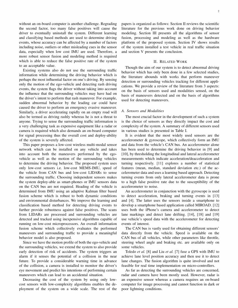
The eye tracking results are shown in Fig. 19i and riskof collision is plotted in Fig. 19j. The collision alarm ringsat three intervals, at 14, 37 and 116s. The first alarm ringswhen the vehicle maintains less than the steering distancefrom the preceding vehicle as shown in Fig. 20a. The secondalarm rings when the driver is looking in the right side mirrorand slowly drifting the vehicle towards the right whereas thislane change will put him within 2 seconds of collision witha vehicle already present in that lane as shown in Fig. 20c.This scenario clearly signifies the importance of eye trackingas the collision potential was detected premature to the lanedeparture. The third alarm rings again when the distance isless than the steering distance as shown in Fig. 20b.
V. CONCLUSION
In this paper we have proposed a multi-modal wirelesssensor network which is able to model the driving behavior
(a) Risk Alarm 1 (b) Risk Alarm 2
(c) Risk Alarm 3
Fig. 20: Situations of Collision Warning Alarm
of the driver as well as provide early detection of risk ofaccidents. The emphasis has been on using low cost sensorsand developing low complexity algorithms that can be run onlow cost microprocessors. The system uses a low cost IMU inconjunction with a low cost GPS to determine the maneuversperformed by the car with the help of machine learning and astate machine. LIDAR sensors are used to detect motion of thesurrounding traffic and a camera to detect the eye movementof the driver. The communication protocol is also proposedwhich ensures seamless flow of messages between relatednodes. Using the information of the surrounding traffic andthe maneuvers performed, the driving behavior of the driver isdetermined, and by using the surrounding traffic informationand driver’s eye tracking, risk of collision is determined.
The system is tested on a real test vehicle. Maneuverdetection accuracy is 100% proving robustness to false alarms.Surrounding traffic information has been shown to benefitboth driver behavior modeling and accident risk detection.Eye tracking helps to reduce the prediction time of thesystem and benefit in timely intervention of potential accidentsituations. All the algorithms ran successfully on low costmicrocontrollers thus completing the objectives of the study.
REFERENCES
[1] NHTSA Press Release. Traffic fatalities fall in 2014, but early estimatesshow 2015 trending higher, November 24, 2015.
[2] Jeffrey S Hickman and E Scott Geller. Self-management to increasesafe driving among short-haul truck drivers. Journal of OrganizationalBehavior Management, 23(4):1–20, 2005.
[3] How-am-i-driving bumper stickers and online driversafety training. Available at dmvreportcard.com/How-Am-I-Driving-Safety-Bumper-Stickers.html.
[4] Derick Johnson, Mohan M Trivedi, et al. Driving style recognition usinga smartphone as a sensor platform. In Intelligent Transportation Systems(ITSC), 2011 14th International IEEE Conference on, pages 1609–1615.IEEE, 2011.
[5] Ravi Kumar Satzoda, Sebastien Martin, Minh Van Ly, Pujitha Gunaratne,and Mohan Manubhai Trivedi. Towards automated drive analysis: Amultimodal synergistic approach. In Intelligent Transportation Systems-(ITSC), 2013 16th International IEEE Conference on, pages 1912–1916.IEEE, 2013.
[6] Asher Bender, Gabriel Agamennoni, James R Ward, Stewart Worrall,and Eduardo M Nebot. An unsupervised approach for inferring driverbehavior from naturalistic driving data.

18
[7] Jiang Liu, Baigen Cai, Jian Wang, and Wei ShangGuan. Gnss/ins-basedvehicle lane-change estimation using imm and lane-level road map. InIntelligent Transportation Systems-(ITSC), 2013 16th International IEEEConference on, pages 148–153. IEEE, 2013.
[8] Rafael Toledo-Moreo, Miguel Zamora-Izquierdo, Antonio F Gomez-Skarmeta, et al. Multiple model based lane change prediction for roadvehicles with low cost gps/imu. In Intelligent Transportation SystemsConference, 2007. ITSC 2007. IEEE, pages 473–478. IEEE, 2007.
[9] Haluk Eren, Semiha Makinist, Erhan Akin, and Alper Yilmaz. Estimat-ing driving behavior by a smartphone. In Intelligent Vehicles Symposium(IV), 2012 IEEE, pages 234–239. IEEE, 2012.
[10] Johannes Paefgen, Flavius Kehr, Yudan Zhai, and Florian Michahelles.Driving behavior analysis with smartphones: insights from a controlledfield study. In Proceedings of the 11th International Conference onmobile and ubiquitous multimedia, page 36. ACM, 2012.
[11] Vygandas Vaitkus, Paulius Lengvenis, and Gediminas Zylius. Drivingstyle classification using long-term accelerometer information. InMethods and Models in Automation and Robotics (MMAR), 2014 19thInternational Conference On, pages 641–644. IEEE, 2014.
[12] Luis M Bergasa, Daniel Almerıa, Jon Almazan, J Javier Yebes, andRoberto Arroyo. Drivesafe: An app for alerting inattentive driversand scoring driving behaviors. In Intelligent Vehicles SymposiumProceedings, 2014 IEEE, pages 240–245. IEEE, 2014.
[13] Minh Van Ly, Sebastien Martin, and Mohan Manubhai Trivedi. Driverclassification and driving style recognition using inertial sensors. InIntelligent Vehicles Symposium (IV), 2013 IEEE, pages 1040–1045.IEEE, 2013.
[14] Dejan Mitrovic. Reliable method for driving events recognition. In-telligent Transportation Systems, IEEE Transactions on, 6(2):198–205,2005.
[15] Jerome Maye, Rudolph Triebel, Luciano Spinello, and Roland Siegwart.Bayesian on-line learning of driving behaviors. In Robotics andAutomation (ICRA), 2011 IEEE International Conference on, pages4341–4346. IEEE, 2011.
[16] Claire D Agostino, Alexandre Saidi, Gilles Scouarnec, and Liming Chen.Learning-based driving events recognition and its application to digitalroads.
[17] Pranaw Kumar, Mathias Perrollaz, Stephanie Lefevre, and ChristianLaugier. Learning-based approach for online lane change intentionprediction. In Intelligent Vehicles Symposium (IV), 2013 IEEE, pages797–802. IEEE, 2013.
[18] Dominik Dorr, David Grabengiesser, and Frank Gauterin. Online drivingstyle recognition using fuzzy logic. In Intelligent Transportation Systems(ITSC), 2014 IEEE 17th International Conference on, pages 1021–1026.IEEE, 2014.
[19] Takashi Bando, Kana Takenaka, Shogo Nagasaka, and TakafumiTaniguchi. Generating contextual description from driving behavioraldata. In Intelligent Vehicles Symposium Proceedings, 2014 IEEE, pages183–189. IEEE, 2014.
[20] Anup Doshi, Brendan Morris, and Mohan Trivedi. On-road predictionof driver’s intent with multimodal sensory cues. IEEE PervasiveComputing, (3):22–34, 2011.
[21] Massimo Canale and Stefano Malan. Analysis and classification of hu-man driving behaviour in an urban environment*. Cognition, Technology& Work, 4(3):197–206, 2002.
[22] Hiren M Mandalia and Mandalia Dario D Salvucci. Using supportvector machines for lane-change detection. In Proceedings of the HumanFactors and Ergonomics Society Annual Meeting, volume 49, pages1965–1969. SAGE Publications, 2005.
[23] Ryota Terada, Hiroyuki Okuda, Tatsuya Suzuki, Kazuyoshi Isaji, andNaohiko Tsuru. Multi-scale driving behavior modeling using hierarchi-cal pwarx model. In Intelligent Transportation Systems (ITSC), 201013th International IEEE Conference on, pages 1638–1644. IEEE, 2010.
[24] Paul J Besl and Neil D McKay. Method for registration of 3-d shapes. InRobotics-DL tentative, pages 586–606. International Society for Opticsand Photonics, 1992.
[25] Robert Kastner, Tobias Kuhnl, Jannik Fritsch, and Christian Goerick.Detection and motion estimation of moving objects based on 3d-warping. In Intelligent Vehicles Symposium (IV), 2011 IEEE, pages48–53. IEEE, 2011.
[26] Chieh-Chih Wang, Charles Thorpe, and Arne Suppe. Ladar-baseddetection and tracking of moving objects from a ground vehicle at highspeeds. In Intelligent Vehicles Symposium, 2003. Proceedings. IEEE,pages 416–421. IEEE, 2003.
[27] Roman Katz, Juan Nieto, and Eduardo Nebot. Probabilistic schemefor laser based motion detection. In 2008 IEEE/RSJ International
Conference on Intelligent Robots and Systems, pages 161–166. IEEE,2008.
[28] Dave Ferguson, Michael Darms, Chris Urmson, and Sascha Kolski.Detection, prediction, and avoidance of dynamic obstacles in urbanenvironments. In Intelligent Vehicles Symposium, 2008 IEEE, pages1149–1154. IEEE, 2008.
[29] Anna Petrovskaya and Sebastian Thrun. Model based vehicle detectionand tracking for autonomous urban driving. Autonomous Robots, 26(2-3):123–139, 2009.
[30] Christoph Mertz, Luis E Navarro-Serment, Robert MacLachlan, PaulRybski, Aaron Steinfeld, Arne Suppe, Christopher Urmson, NicolasVandapel, Martial Hebert, Chuck Thorpe, et al. Moving object detectionwith laser scanners. Journal of Field Robotics, 30(1):17–43, 2013.
[31] Michael Bosse and Robert Zlot. Map matching and data association forlarge-scale two-dimensional laser scan-based slam. The InternationalJournal of Robotics Research, 27(6):667–691, 2008.
[32] Takashi Ogawa, Hiroshi Sakai, Yasuhiro Suzuki, Kiyokazu Takagi, andKatsuhiro Morikawa. Pedestrian detection and tracking using in-vehiclelidar for automotive application. In Intelligent Vehicles Symposium (IV),2011 IEEE, pages 734–739. IEEE, 2011.
[33] Kimberly Tuck. Tilt sensing using linear accelerometers. FreescaleSemiconductor Application Note AN3107, 2007.
[34] T Talat Ozyagcilar. Implementing a tilt-compensated ecompass usingaccelerometer and magnetometer sensors, freescale semiconductor ap-plication note,(2012), n. AN4248, rev, 3.
[35] Fawzi Nashashibi and Alexandre Bargeton. Laser-based vehiclestracking and classification using occlusion reasoning and confidenceestimation. In Intelligent Vehicles Symposium, 2008 IEEE, pages 847–852. IEEE, 2008.
[36] Fabian Timm and Erhardt Barth. Accurate eye centre localisation bymeans of gradients. VISAPP, 11:125–130, 2011.
[37] Paul Viola and Michael Jones. Rapid object detection using a boostedcascade of simple features. In Computer Vision and Pattern Recognition,2001. CVPR 2001. Proceedings of the 2001 IEEE Computer SocietyConference on, volume 1, pages I–511. IEEE, 2001.
[38] Jonas Jansson. Collision avoidance theory: With application to automo-tive collision mitigation. 2005.
[39] Ethem Alpaydin. Introduction to machine learning. MIT press, 2014.
Hamad Ahmed completed B.Sc. in Electrical En-gineering from University of Engineering and Tech-nology, Lahore in 2015 with majors in Telecom-munication and Electronics Engineering. Currently,he is working as a research assistant in the Sig-nal Processing & Navigation Algorithms Group atthe Department of Electrical Engineering, LahoreUniversity of Management Sciences on the devel-opment of low cost alternatives to GPS for vehiclelocalization. His research interests lie in the areasof Statistical Signal Processing, Optimal Estimation
Theory, Wireless Sensor Networks and Machine Learning.
PLACEPHOTOHERE
Muhammad Tahir Biography text here.