a machine-learning approach to keypoint detection and · pdf file ·...
TRANSCRIPT
Int J Comput VisDOI 10.1007/s11263-012-0605-9
A Machine-Learning Approach to Keypoint Detectionand Landmarking on 3D Meshes
Clement Creusot · Nick Pears · Jim Austin
Received: 14 October 2011 / Accepted: 17 December 2012© Springer Science+Business Media New York 2013
Abstract We address the problem of automaticallydetecting a sparse set of 3D mesh vertices, likely to be goodcandidates for determining correspondences, even on softorganic objects. We focus on 3D face scans, on which sin-gle local shape descriptor responses are known to be weak,sparse or noisy. Our machine-learning approach consists ofcomputing feature vectors containing D different local sur-face descriptors. These vectors are normalized with respectto the learned distribution of those descriptors for some giventarget shape (landmark) of interest. Then, an optimal func-tion of this vector is extracted that best separates this par-ticular target shape from its surrounding region within theset of training data. We investigate two alternatives for thisoptimal function: a linear method, namely Linear Discrim-inant Analysis, and a non-linear method, namely AdaBoost.We evaluate our approach by landmarking 3D face scansin the FRGC v2 and Bosphorus 3D face datasets. Our sys-tem achieves state-of-the-art performance while being highlygeneric.
Keywords keypoint detection · landmarking · 3D facerecognition · Machine learning · LDA · AdaBoost
C. Creusot (B) · N. Pears · J. AustinDepartment of Computer Science, University of York, York, UKe-mail: [email protected]
N. Pearse-mail: [email protected]
J. Austine-mail: [email protected]
1 Introduction
Searching for corresponding points (correspondences) acrossa pair of shapes is an essential early process for a large numberof applications involving 2D images, 3D meshes and multi-modal systems that use a mixture of both. For example, instereo vision, structure-from-motion and tracking objects invideo, we need to establish pairs of image points that cor-respond to the same scene point. Establishment of 3D pointcorrespondences is often required for 3D shape registrationand matching, particularly in the case of partial views (therear faces of 3D shapes are not captured in 2.5D scans). Theseprocesses are essential components of 3D object retrieval and3D shape recognition systems.
Since the determination of correspondences is a searchproblem, with O(n2) complexity, a reduction in the searchspace by detecting a sparse set of keypoints1 is common prac-tice. The use of corner detectors is the classic example of thisin 2D images, while a locally extremal value of Gaussian cur-vature is commonly used on 3D meshes.
Note that a keypoint is an unlabeled point and a goodkeypoint detector generates outputs at pairs of points withlocally similar shapes across a pair of similar 2D images or3D scans. At the same time, the detector should generate asfew as possible outputs in the overlapping region of the twoimages or scans that are not part of a valid correspondence.
Often keypoints are used directly to determine correspon-dences between a pair of 2D images or a pair of 3D scans ofthe same scene object. Keypoints can also be used to initialisethe pose and shape parameters of a generic shape model, suchas a 3D morphable face model. In this case, a sparse set ofreliably detectable landmarks is selected (usually manually)on the generic shape model and these are the points that we
1 Also called interest points or feature detections in other literature.
123

Int J Comput Vis
aim to match extracted keypoints to. We can view the sparseset of landmarks as a subset of a relatively dense genericshape model and we encapsulate this small subset of pointsand their relative positions in an entity called a landmarkmodel, L. This model is annotated with L landmarks, wherelandmarks have both a position and a label. Hence, in con-trast to keypoints, they are labeled points.2 When keypointsare the inputs of a labeling system, they are seen as land-mark candidates and are usually associated with a list ofpossible candidate landmark labels. Often, the initial map-ping between query scan keypoints and model landmarksis many-to-many. However, once a one-to-one correspon-dence is established between a keypoint on a query scan anda landmark on the model, L, a keypoint may ‘acquire’ theassociated model label and is then upgraded to a landmark.3
Thus the landmarking process usually contains two mainparts: detecting keypoints on a query, which usually pro-vides many landmark candidates, and eventually selectingn of these, up to a maximum of the total number of modellandmarks, the actual number depending on the degree ofocclusion on the query scan. Detecting the keypoints andcomputing the correspondences with the landmark model’slabels are two different problems. The keypoint detection canbe seen as a local-only (featural) problem while the corre-spondence search takes into account both local (featural) andglobal (configural) information. This paper is mainly focusedon the detection of keypoints on 3D scans as probable land-mark candidates. However, in Sect. 6, we present a methodthat uses our keypoint detector in a complete 3D face land-marking system and we compare it to the state-of-the-art inorder to demonstrate the high performance and generality ofour approach.
Captured 3D scans have several advantages over 2Dimages; for example, scale changes are often not so pro-nounced for some object class and it is easier to deal withpose and illumination variations. However, they also havea set of specific drawbacks. For example, if one comparesa 2D image and 3D depth map of a soft, organic structuresuch as a human face, there appears to be a larger number ofsalient structures in the 2D image, which could be localizedby standard 2D keypoint detectors. However, the applica-tion of a standard keypoint detector on a 3D scan, such aslocally extremal Gaussian curvature, leads to a highly sparseset of keypoints. This is the main motivation for buildingour machine learning based keypoint detection system. Animportant aspect of our keypoint detector, that allows its gen-eral deployment, is that it can generate useful keypoints over
2 It is essential that the reader distinguishes carefully between unlabeledkeypoints and labeled landmarks throughout this paper.3 To be more precise, a query scan point close to an extracted keypointis sometimes designated to be the landmark, in order to minimize theleast-squares error when fitting model L. This is discussed in Sect. 6.
large regions of soft, organic shapes, as there is no require-ment for a keypoint to exist at the locally extremal valueof any single, scalar local shape descriptor4 (e.g. Gaussiancurvature).
Rather, a set or dictionary of L local shapes is learned,where each member of the dictionary is associated with aparticular landmark that is labeled across a set of trainingmeshes. Subsequently, keypoints can be generated on querymeshes, where the local shape is highly similar to one of themembers of this dictionary.
Although many researchers have developed systems todetect facial features in 2D images, using well-definedmachine learning techniques, researchers working with 3Dfaces have almost exclusively developed heuristic approachesthat rely on restrictive assumptions, such as a near-frontalpose. These approaches are usually landmark dependentsequential recipes taking advantage of patterns detected bytheir designers. Such a recipe can be, for example, to take thetip of the nose as the most extreme point along one directionor as the maximal convex curvature in the query scan. Theserecipes give very good results for very salient points on mostexisting datasets, but are bound to fail on some scans of non-cooperative subjects; for example, when the assumption of anear-frontal pose is broken or when the nose tip is occluded.
In summary, the main contribution of this paper is ageneric keypoint detection process for 3D meshes, based onmachine learning, which is then employed in a 3D face land-marking system in order to improve upon existing heuristicapproaches. In our system, detector functions are learnedrather than being enforced by the designer of the system.This allows:
1. generality, as all of the landmarks are processed with thesame general framework;
2. a more reliable detection of landmarks when the inputdata is not cropped (e.g. when there are non-facial ele-ments in a face capture);
3. an intrinsic robustness to missing data, because we do notfollow a sequential progression through the landmarks.Most other landmarking systems will fail if the nose orthe inner eye corners are missing, as these strong featuresare often used to search for weaker, less salient features;
4. the detection of less salient features for which humandesigners struggle to create detection functions or rules(e.g. corners of the mouth and outer corners of the eyeson the human face).
4 We define a scalar local shape descriptor as a real number thatdescribes the shape of the local neighborhood surrounding some meshvertex. In some literature, this is termed a feature or feature descriptor.Here, the local neighborhood is Euclidean and enclosed by a sphere ofpredefined radius.
123

Int J Comput Vis
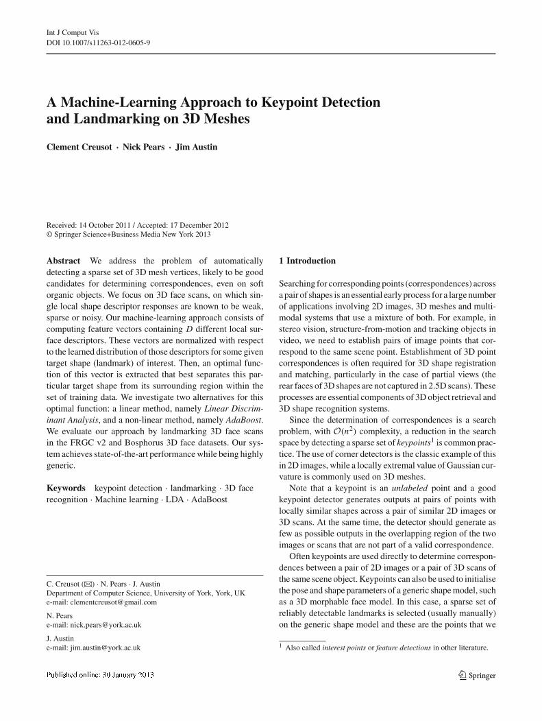
Fig. 1 Example of keypoint detection using our method on a 3D scan from the FRGC dataset
Fig. 2 Problem breakdown.The landmarking problem issplit into two sub-problems thatare solved independently:keypoint detection and labeling.Although this paper mainlyfocuses on solving the keypointdetection problem, we alsoapply our technique in alandmarking problem
Specific contributions on a practical level are:
1. a new method for keypoint detection on meshes, using adictionary of L learned local shapes (see Fig. 1);
2. an evaluation of its performance using two differentapproaches to generate functional forms of local shapedescriptors, linear (LDA) and non-linear (AdaBoost);
3. a new framework for 3D mesh landmarking based onautomatically detected keypoints (see Fig. 2).
The work presented here is an extension of our workin Creusot et al. (2011) and is structured as follows. In thefirst section, previous work on keypoint detection and land-marking of 3D meshes is reviewed. In the following overviewsection, Sect. 3, we give our problem definition and we out-line the offline training and online testing processes of oursolution. Here, we also discuss our datasets and performancemetrics used for evaluation. In the following section, wepresent the fine detail of our machine learning approach tokeypoint detection on 3D meshes. In Sect. 5, we evaluatethis keypoint detection system, while the following sectiondescribes its application to landmarking. A final section isused for conclusions.
2 Previous Work
Unlike tracking and stereo-vision applications, or matchinggeneric salient points across 3D shapes, landmarking requirescandidate positions that are close to the targeted human-defined landmarks required for a particular application. Thisis usually achieved through an expert system approach: thesystem designer (expert) will notice a correlation betweenthe local shape of the mesh and the targeted landmark anduse this observed correlation to define some heuristic rule toselect candidate positions on new queries. For example, theexpert will observe that the position of the nose tip is oftencorrelated with the highest convex curvature points in thecentral facial area or that the nose is the closest point to thecamera or the most extremal point in a particular direction.Unfortunately, rules extracted from such observations won’talways work in the general case, as the input may contain arti-facts other than the face, such as hair, hands and accessories(e.g. hats, glasses).
2.1 Landmark Candidate Detection on 3D Faces
A scalar descriptor of some specific type can be computedat every vertex of a mesh. Typically these values are color
123

Int J Comput Vis
mapped and rendered over the mesh to give a visualizationof how the descriptor responds to the local shapes within themesh. Such a visualization is termed a descriptor map (or,in some literature, a feature map). It can be thought of as ascalar field over the scanned object’s surface that is sampledat the vertices of the mesh.
The use of descriptor maps on 3D meshes, such asGaussian curvature maps, is common practice to detectlandmark candidates. A typical multiple landmark detec-tion approach is presented in Colbry et al. (2005). First, theauthors preprocess the face to remove spikes, before croppingthe upper part of the scan as being the region of interest. Thenthe nose is localized as the closest vertex to the camera, orthe most extreme point in a particular direction (left or right),or the one with the largest shape index. The inner eyes cornerare detected as the points with the smallest shape index. Thiskind of approach has a lot of variants and is widely used inboth academic and commercial systems.
Other authors have noticed that the sagittal slice of theface remains identical over orientation changes and there-fore can be used to detect the nose. In Faltemier et al. (2008),contours of the mesh are extracted at varying angles until itmatches a previously learned nose profile signature. The sys-tem achieved a 98.52 % accuracy on the NDOff2007 3D facedataset, for the nose tip with variations of angle up to 90◦.(This dataset contains a total of 6,911 non-frontal images con-taining neutral expressions and a single frontal neutral imagefor each of 406 distinct subjects.) Some non pose-invarianttechniques have also used transverse slices to detect the nosetip and the nose corners (Segundo et al. 2007; Mian et al.2006).
To summarize, most papers on 3D face landmarking havetheir keypoint detection system grouped in one of the follow-ing categories:
– curvature/volume extrema: the candidates are defined asextrema over curvature and/or volume based descriptormaps (Chang et al. 2006; Colbry et al. 2005; D’Hoseet al. 2007; Pears et al. 2010; Romero and Pears 2009;Segundo et al. 2007; Szeptycki et al. 2009).
– directional extrema: the candidates are defined as theextremal points in given directions (Chang et al. 2006;D’Hose et al. 2007). This is only used for the nose tipdetection.
– 2D curve extrema: by using profiles and slicing ofthe mesh, the detection of salient points is reduced tofinding extremal points along a two-dimensional curve(Faltemier et al. 2008; Mian et al. 2006; Segundo et al.2007).
Several previous studies have acknowledged the lim-itations imposed by heuristic approaches and employedmachine learning techniques instead (Berretti et al. 2010;
Zhao et al. 2011). However, they usually employed 2Ddescriptors on depth maps making their systems unusablein scenarios presenting a large rotation from the frontalview. To the best of our knowledge, it appears that no 3Dmachine learning method exists for facial landmark candi-date (keypoint) detection (see Fig. 3). This is a gap in theliterature that we aim to fill, to enable better landmarkingon face scans of non-cooperative subjects. Clearly, this hasgreat utility in high-throughput 3D face recognition systemsthat do not require subject cooperation. Our proposed systemis sufficiently generic to be applied to meshes of other gen-eral classes of objects, in any application where landmarksof interest can be manually defined on a set of training scans.
2.2 Keypoint Detection on Faces
Keypoints on 3D faces are often not labeled and, typically,they are used for the purpose of face recognition. In thesecases, the desired keypoints are repeatable for a given iden-tity but differ from one individual to another. For example,Mian et al. (2008) use a coarse curvature-related descrip-tor to detect such keypoints, while in Berretti et al. (2010)and Mayo and Zhang (2009), they are computed using theScale-Invariant Feature Transform (SIFT Lowe 2004) on 2Ddepth-maps.
In this paper, the term keypoint is justified as we try todetect unlabeled repeatable point of interest. However, ourapproach differs, as the scope for the targeted repeatabilityis larger. Our technique should be able to detect repeatablepoint of interest across the population and not only for sev-eral captures of the same individual. Therefore, our system isdesigned to extract macro-features (nose, eyes, mouth) com-mon across a whole population of objects (faces), instead ofdiscriminative micro-features (e.g. wrinkles) that are oftenspecific to individuals.
2.3 Keypoint Detection and Landmarking on Other Objects
Computing keypoints in order to determine correspondencesis useful for all kinds of object matching applications. Shaperetrieval (e.g. in web search applications) is one such applica-tion and there is now a robust feature detection and descrip-tion benchmark, the SHREC benchmark (Boyer et al. 2011),that tests the performance of feature detectors and descriptorsunder a variety of transformations, such as scaling, affine andisometry (bending) transformations, and a variety of noiseconditions.
In Mian et al. (2010), keypoints are computed using acoarse curvature descriptor to localize objects in scenes withocclusions. In Zaharescu et al. (2009), an approach calledMesh DoG is presented. This is a multi-scale approach thatmakes use of Difference-of-Gaussians (DoG), and thus hassimilarities to the DoG approach applied to 2D images in
123

Int J Comput Vis
Fig. 3 Related work: facial landmark candidate detection usually appears as a single section in face landmarking papers. Most of them are sequentialrecipes. Some use machine learning techniques but in these cases, they are always with 2D representations (e.g. SIFT Lowe 2004 on depth maps)
the SIFT descriptor (Lowe 2004). In this approach, any sur-face descriptor map can be convolved with a set of Gaussiankernels of different scales (standard deviations). Subtractingconvolutions across two adjacent scales gives the DoG oper-ator response. Keypoints are then extracted as the local max-ima across scale space, using non-maximal suppression in aone-ring neighborhood in the current and adjacent scales. Asimilar DoG-based approach is presented in Castellani et al.(2008). However, here the DoG operator is applied to theactual mesh over a range of scales. The amount that a vertexmoves between Gaussian filtering at one scale and the nextis projected along the vertex normal. Keypoints are extractedas points of maximal normal movement over local neighbor-hoods and local scales.
In Ben Azouz et al. (2006), landmarking of 3D humanmodels is addressed. Here a graphical model is created, withlandmarks at the graphical nodes being characterized by spinimages (Johnson and Hebert 1999). Functions express thelikelihood that a particular landmark corresponds to a givenvertex on the query mesh (based on the distribution of learnedspin images in the model). Other functions constrain a pair oflandmarks to be consistent with their learned spatial relation-ship in the model. To perform the optimization of landmarkassignment, the authors employ a belief propagation algo-rithm. An interesting aspect of this approach is that it doesnot use a keypoint extraction phase to reduce computationtime. Encouraging results are obtained on a very small testset (30 scans).
In Itskovich and Tal (2011), two kind of curvature-relateddescriptor (shape index and Willmore energy) are combinedto detect the keypoints on archaeological objects in order todetect regions matching a given pattern. This paper is oneof the rare case where more than one local shape descrip-tor is used for the keypoint candidate selection. An otherexample is Dibeklioglu et al. (2008) where shape index, dif-ference map, and image gradient are combined for landmarklocalization. Besides, when several such scalar descriptorsare used, combining them is usually done using fixed coeffi-cients.
In this paper, a framework is presented to determineautomatically how descriptors should be combined for eachlandmark in landmark model L, designed for the specificproblem of 3D face landmarking.
3 Overview
In this section, we give the problem statement, outline oursolution and the methodology for its evaluation.
3.1 Problem Statement
The main problem that we address is the detection and subse-quent labeling of points on input 3D meshes that are locallysimilar to at least one member of a set of L predefined land-marks in a landmark model (see Fig. 1).
123

Int J Comput Vis
This statement implies that the landmarked points shouldbe a subset of the input mesh’s vertices. This can be justifiedin our case by the fact that the resolution of the input meshis good enough compared to the acceptable error in position-ing. ‘Sub-vertex’ localization of landmarks (i.e. to a higherresolution than the input mesh) is an interesting problem forlandmark refinement techniques, but is not discussed in thispaper. Rather, our aim is to enable the system to automati-cally learn functions of a set of D local shape descriptors,extracted over a set of training meshes, that enable robustkeypoint detection on unseen input meshes.
3.2 Outline of the Keypoint Detection System
We define L = 14 landmarks in a landmark model L, asshown in Fig. 4. In each of a set of N training meshes, theseL landmarks are manually localized with a point-and-clickinterface.
To implement our system, we need to define what kind oflocal shape descriptors to use. The use of a single scalar 3Dlocal descriptor on its own is usually not very discriminative.Therefore, we use a set of D (10–48) scalar shape descriptorsincluding, for example, Gaussian curvature, mean curvatureand a volumetric descriptor (details given in Sect. 4.1). Afternormalization to a set of scores (which range from 0 to 1),these form a feature vector that describes local shape at somemesh vertex. (It can be thought of as a D-dimensional vec-torial descriptor, which is composed of a collection of scalardescriptors.)
Our framework is composed of an offline training processand an online keypoint detection process, as illustrated inFigs. 5 and 6 respectively, and we now describe each of theseprocesses in turn.
3.2.1 The Offline Training Process
Figure 5 shows the offline training process, which is usedto teach the system what is considered to be a shape ofinterest. The inputs to this training system are a set of Ntraining meshes and an associated set of L landmarks per
Fig. 4 Position of the 14 landmarks, centers of our local shapes ofinterest for the training part of the system
training mesh, where each specific landmark, λ (e.g. nosetip), has a vertex index, i , within a training mesh. Withinour system, D local shape descriptors are defined and wecan process an arbitrary number of such descriptors, up tosome limit imposed by memory and computation time lim-itations. The following four broad steps outline our trainingprocess.
1. For every training mesh, D descriptor maps are gener-ated, where a descriptor map is defined as the raw descrip-tor values, xd , d ∈ {1 . . . D}, computed over all verticesof a training mesh.
2. Then, for each landmark, λ ∈ {1 . . . L}, we collect theN raw descriptor values over the N training meshes andestimate the parameters of their distributions (we primar-ily use Gaussian distributions, see Sect. 4.2.1).
3. These learned statistical distributions allow us to map rawdescriptor values into normalized descriptor-landmarkscores or DL-scores. (In terms of visualizations, DL-score maps are generated from descriptor maps.) Suchscores are specific to a descriptor-landmark, (d, λ), pairand hence there are D× L of these per vertex per trainingmesh (see Fig. 5). To generate these scores, over all ver-tices of a training mesh, the raw values, xd , of descriptord are projected against the distribution of xd at land-mark λ and normalized by the probability density func-tion (pdf) maximum of the distribution. Scores close to 1are obtained if the descriptor value is close to the modalvalue of the distribution, and scores close to zero areobtained if the descriptor is far from that modal value.
4. Effectively, these D scores, computed with respect to thedistributions at some landmark, λ ∈ {1 . . . L}, form aD-dimensional feature vector at every vertex across alltraining meshes. We can form two classes of such fea-ture vectors: those from vertices that are close to land-mark λ across all of the training meshes and those fromsurrounding vertices that are more remote from the samelandmark. An example of the two classes employed isshown in Fig. 7, where neighboring vertices of the upperlip landmark are shown in blue and the non-neighboringclass of vertices is shown in red. (Note that this is onlyshown for one face scan, but these classes are formed bythe union of all such vertices across the full training set.)We then learn the function operating on these feature vec-tors that best discriminates between these two classes. Ineffect, this is a detector function, fλ, and there is one foreach landmark, λ. In the case of LDA, this detector func-tion is a linear combination of the elements of the featurevector, whereas a non-linear function is generated usingAdaBoost.
To summarize the training process, L landmarks labeledover each mesh in a training set are used to define a dictionary
123

Int J Comput Vis
of local shapes where, for each shape, both the statisticaldistributions of shape descriptors and the rules for combiningsuch descriptors are learned. The concept of this dictionaryis illustrated by the red boxes in Figs. 5 and 6
It is important to note that the normalization of DL-scoresin step 3 is not essential to apply our machine learningprocesses in step 4. Learning of the detector function couldbe applied directly to the raw descriptor values, as one mightexpect when using a powerful classifier such as AdaBoost.
In fact in Creusot (2011)[p. 150–152], we compare detectorfunctions learned from scores against those learned from rawdescriptor values. We found that the performance was verymarginally better for scores, but the difference was so smallas to not be significant. (In more detail: for 6 landmarks,scores gave marginally better performance, for 3 landmarks,raw descriptors gave marginally better performance and for 5landmarks the performance was almost identical.) However,improved detector functions was never the intention of using
Fig. 5 Offline process: knownlandmark positions on thetraining set are used to learnidealized distributions(parameterized class-conditionalprobability density functions) ofthe descriptor values for eachshape of interest. The matchingscores computed using thosedistributions are used to train thedescriptor combination systemfor every landmark as explainedin Sect. 4.3
Fig. 6 Online process: Ddescriptor maps are computedfrom the input mesh, each valueis matched against the L learneddescriptor distributions (14) toget score maps with valuesbetween 0 and 1. For eachlandmark, the D descriptorscore maps are combined usingthe learned combination rulesand renormalized to span therange (0–1). The L normalizedlandmark score maps arecombined into a single finalkeypoint score map, using themaximal value (of L values) ateach vertex. The outputkeypoints are the strongest localmaxima detected on thiskeypoint score map that areabove some given threshold T
123

Int J Comput Vis
Fig. 7 Example of vertex class generation, showing neighboring (blue)and non-neighboring (red) vertices for the upper-lip landmark on oneface of the training set
scores when we developed our framework. Rather, we claimthe following advantages:
– Scores normalize descriptor values to compatible ranges,thus giving a great deal of insight to the researcher aboutthe inner workings of the classification technique allow-ing us to rapidly know which descriptors are good touse and for what landmarks they should be employed(Creusot et al. 2011).
– Scores make visualization of results much easier, as wit-nessed by the colormap graphics in this paper.
– Scores allow histogram descriptors and scalar descriptorsto be used in the same framework at the same time. Alltypes of descriptor are converted to the same space (a unithypercube), which make it possible to use very hetero-geneous types within the same framework. This is a realstrength of our framework in terms of its extensibility.
3.2.2 The Online Keypoint Detection Process
The online part of our system takes a previously unseen facemesh as its input. The process is composed of the followingstages, see Fig. 6.
1. D local shape descriptors (scalars, e.g. Gaussian curva-ture) are computed for all V vertices in the input mesh.
2. For each of the L learned local shapes:
– D Descriptor-Landmark score (DL-score) maps arecomputed by projecting the descriptor values of eachvertex against the associated learned distributionsof the target landmark. The scores generated arebetween 0 and 1. A value of 1 is generated when thevalue of the descriptor is equal to the maximum of thelearned distribution (modal value). These normalizedscores are collected together into a D-dimensional
descriptor, or feature vector, at each vertex of theinput mesh.
– Using the learned detector function, fλ, for landmarkλ in the training phase, a (scalar) response is gen-erated, which we call a landmark score. The land-mark score map is then normalized over the mesh toensure the matching scores associated with differentlandmark shapes have the same impact on the finalkeypoint extraction stage. This normalization ensuresthat the landmark score map has values ranging from0 to 1.
3. All of the landmark score maps are combined into onefinal keypoint score map, by using the maximum value(over all L landmark dictionary shapes) for each vertex(see Fig. 14).
4. The keypoints are defined as the strong local maximaon this final keypoint score map. A threshold T is usedto discard weak candidates. The maximum number ofkeypoint retained is limited to 1 % of the total number ofvertices.
This completes the outline of our system. A more detaileddescription of our keypoint detection system is presented inSect. 4 and describes the descriptors employed and imple-mentation details. The remainder of this section describesthe datasets (Sect. 3.3) and performance metrics (Sect. 3.4)that we use for evaluation.
3.3 Datasets
Our keypoint detection system, described above, is testedon the Face Recognition Grand Challenge version 2 (FRGCv2) dataset (Phillips et al. 2005) containing 4,950 faces of557 individuals. This data contains both males and femaleswith some variation in ethnicity, age and expression as wellas small variations in pose (under 10◦). The dataset is fairlyuneven in terms of capture per identity with some individualsappearing only once while others appear thirty times. Thisdataset is widely used in the research community and, overthe years, has become a standard benchmark for 3D faceprocessing systems.
The input data for our system is lower resolution than theoriginal structured point cloud (640 × 480 vertices). Thepoint density is reduced by replacing each block of 4×4 raw3D data points with its average. A mesh is then created bydefining two triangular faces for every group of four adjacentvertices .
For the landmarking experiments, both the FRGC and theBosphorus dataset Savran et al. (2008) are used. The Bospho-rus dataset contains 4,666 captures of 105 people. Unlikethe FRGC, it contains large variations in pose and occlu-sions (hands, hair and glasses partially covering the face). In
123

Int J Comput Vis
the landmarking experiments, for which time performance ismeasured, the point density of the original input data in bothdatasets is reduced by binning the points into square pixelsof fixed size 3.5 mm . Compared with the aver-aging method, this allows us to reduce even further the pointdensity (and therefore the computation time), while keepinga fixed resolution whether the face is captured from a closeor remote position.
For the FRGC dataset, 200 neutral expression scans of dif-ferent individuals are selected randomly as our training setand all remaining scans are used as a test set (4,750 faces).The manually-derived ‘ground truth’ landmarks are a mix-ture of contributions from Romero-Huertas et al. (2008) andSzeptycki et al. (2009) with additional manually located land-marks and refinements.
For the Bosphorus dataset, only 99 neutral expressionfrontal scans are used as training, leaving 200 faces in theneutral-frontal test set and 4339 scans in total in the globaltest set.5 The ground-truth landmarks are the ones providedwith the dataset (Savran et al. 2008) with some manual addi-tions (subnasale, nasion) and refinements.
3.4 Performance Metrics
We define three performance metrics to evaluate the per-formance of our systems: the landmark retrieval rate, thelandmark positioning error and the global registration error.Each of these is described in the following three subsections.
3.4.1 Landmark Retrieval Rate
We define the landmark retrieval rate for a particular land-mark as the percentage of test scans in which the system cor-rectly retrieved its position given an error acceptance radius.For example, if the test set contains 1,000 models, amongwhich 990 have a ground truth landmark for the nose tip, andif we use an error acceptance radius of 10 mm, the landmarkretrieval rate will be the percentage of the 990 models whichpresent a detected nose tip landmark within 10 mm of theknown nose tip position.
Usually it is not clear what radius should be used for suchevaluation. As a good practice and to facilitate results com-parison with other researchers, the retrieval rates are pro-vided for a varying acceptance radius (usually increasingfrom 2.5 mm to 25 mm in steps of 2.5 mm).
3.4.2 Landmark Positioning Error
Computing the distance from every localized landmark to theground truth position of the corresponding label is an interest-
5 Subsets R_90, L_90 and I G N of the Bosphorus dataset are not usedin this paper.
ing measure for the global landmark localization framework.However this continuous measure is more meaningful forlandmark positioning refinement than for coarse landmarklocalization. This measure doesn’t allow notions of discretefailure and will only be used in the last section where a com-plete landmarking system is presented.
3.4.3 Global Registration Error
We can register the detected landmarks with the ground truthlandmarks in the same scan. If a scale-adapted rigid registra-tion is used, we expect to see zero rotation, zero translationand a unity scale in the ideal case. Any deviation from theideal values gives a global measure of the landmarking per-formance. This give us an interesting performance metric forthe overall matching.
4 A Machine Learning Approach to Keypoint Detection
In this section, the implementation details of our keypointdetector are presented. When reading this section, it is use-ful to keep the system overview presented in Sect. 3.2 andassociated figures, Figs. 5 and 6, in mind.
4.1 Computation of Descriptors
Our system makes extensive use of local shape descrip-tors; in this section, details about their computation are pre-sented. In our experiments, two kinds of descriptors areused, scalar-valued descriptors (e.g. Gaussian curvature) andvector-valued descriptors. This latter form of descriptor is alocal shape histogram, such as a spin image (Johnson andHebert 1999).
4.1.1 Normals
Several of the descriptors require a normal defined at everyvertex. To compute the normals, a simple method using theadjacent triangle faces is used. When the mesh has been builtfrom the 2D depth map, all the triangle faces have beendefined anti-clockwise with regard to the camera position.Therefore all the normals of the faces are pointing outward.When setting the normal at a vertex i , a weighted sum of thenormals of the neighboring faces is computed. The weightsgiven for each of the adjacent faces are computed using theNelson Max technique (Max 1999):
cni =ne
i∑
j=1
e j × e j+1
|e j |2|e j+1|2 (1)
123

Int J Comput Vis
where ni is the normal vector at vertex i , c is a constant thatdisappears after unit-length normalization, ne
i is the numberof edges adjacent to vertex i and e j the vector correspond-ing to the j th neighboring edge. As the normal is computedat every vertex, the efficiency of the process is improvedby looping over the triangle faces and accumulating the facenormals with the corresponding weights on the three verticesof the face. This guarantees that the face normals are com-puted only once (instead of three times with a naive algorithmlooping on vertices).
4.1.2 Neighborhoods
A point by itself contains very little information: only itsposition in the space. To extract more information one needsto know how this point is positioned with regard to the otherpoints within its local neighborhood. In other words, a quan-titative description of local shape needs to be extracted in away which is invariant to the orientation (pose) of the scannedobject (face) with respect to the 3D camera. This is a functionoperating on a set of vertices contained within a local neigh-borhood.
To determine this local neighborhood,the only thing thatis needed is a metric and a threshold. Here we use a sim-ple Euclidean metric to determine the neighborhood (seeFig. 8) i.e. vertices need to be within a bounding sphere ofsome specified radius that defines neighborhood size. Thechoice of neighborhood size is a compromise. A neighbor-hood that is too small with respect to the raw data reso-lution will lead to local surface properties being noisy orundetermined. On the other hand, if the local region is toolarge, the notion of locality is broken and the descriptor val-
Fig. 8 Neighborhood computed using Euclidean distance. The red lineis the intersection of the sphere of radius R with the surface. Every pointinside the sphere is part of the local neighborhood. The blue verticesrepresent the perimeter (Color figure online)
ues become vulnerable to occlusions. Since the neighbor-hoods depend on a fixed distance, every descriptor using theseneighborhoods cannot be invariant to the scale of the scannedobject.
4.1.3 Principal Curvatures
The curvature is a simple notion of 2D geometry that mea-sures the bending of a curve at a particular point. It is definedas the inverse radius of the osculating circle at that location.This 2D notion can be used with points on a 3D surface byextracting 2D plane curves at those points using an intersect-ing plane. This intersecting plane always contains the normal,leaving one degree of freedom, the angle around the normal,and therefore an infinite number of possible 2D curves andcurvature values. To provide a simple measure of the 3Dsurface curvature, only two angles are selected: the ones giv-ing the maximal and minimal curvature values known as first(k1) and second (k2) principal curvatures (see Fig. 9 for thesedescriptor maps).
Computing these two values for a discrete surface is nottrivial. The curvature computation approach employed isthe Adjacent-Normal Cubic Approximation method proposedin Goldfeather and Interrante (2004).
4.1.4 Descriptors Derived from Principal Curvatures
The two principal curvatures k1 and k2 are rarely useddirectly. Most of the time they are used to compute otherdescriptors. A list of the most commonly used ones is givenbelow:
– Gaussian Curvature (K ):
K = k1k2 (2)
– Mean Curvature (H ):
H = k1 + k2
2(3)
– Shape Index (SI): two variants
SI0,1 = 1
2− 1
πarctan
k1 + k2
k1 − k2, 0 ≤ SI0,1 ≤ 1 (4)
or
SI−1,1 = 2
πarctan
k1 + k2
k1 − k2, −1 ≤ SI−1,1 ≤ 1 (5)
123

Int J Comput Vis
Fig. 9 Examples of descriptor maps for the first (k1) and second (k2) principal curvatures (REucl.scalar = 15 mm) (Color figure online)
– Curvedness (C):
C =√
k21 + k2
2
2(6)
– Log-Curvedness (LC):
LC = 2
πlog
√k2
1 + k22
2(7)
– Willmore Energy (W ):
W = H2 − K = (k1 − k2)2
4(8)
– SC (Kim et al. 2009):
SC = SI−1,1 · LC = 4
π2 log
√k2
1 + k22
2arctan
k1 + k2
k1 − k2
(9)
– Log Difference map (Dibeklioglu et al. 2008):
LD = ln(K − H + 1) = ln(k1k2 − k1 + k2
2+ 1) (10)
Figure 10 shows some examples of scalar descriptor mapson frontal and profile 3D faces.
4.1.5 Local Volume (VOL)
Other kinds of measures that can be made from the localneighborhood are the ones that use volume. First, thebarycenter (point pc(vi )) of the perimeter of the neighbor-hood of vertex vi is determined. Then the volumes of thetetrahedra computed from this point and all the faces of the
neighborhood are summed. Figure 11 shows how the tetra-hedra are computed. As the faces are oriented the volume canbe positive (concave shape) or negative (convex shape).
4.1.6 Distance to Local Plane (DLP)
The distance to local plane is a coarse measure of the con-vexity/concavity at a point (Pears et al. 2010). It is definedas the Euclidean distance between vertex vi and the planefitting its neighboring points. This corresponds to projectingthe vector between the centroid of the neighborhood and thevertex vi onto the normal direction of the plane. In general,the neighborhood used to compute the normal and the neigh-borhood used to compute the target centroid can be different.However, it is usually simpler to take them as equal.
4.1.7 Histogram-based Local Shape Descriptors
Simple scalar descriptors are sometimes limited in terms oftheir ability to describe local surface shape. When dealingwith complex surface shapes, more information is neededthan a simple scalar value. It is possible to build local shapedescriptors using histograms i.e. any array of fixed dimen-sions containing information about the neighboring surfaceat some mesh vertex. These are inherently feature vectors inthemselves, but can be combined, in full or part, with thescalar descriptors described above to form larger and poten-tially more discriminating feature vectors.
Such histogram-based descriptors are often computation-ally expensive. For this reason they are usually only used asdescriptors for matching a sparse set of keypoints, rather thanused for detection of keypoints on a relatively dense set of rawmesh vertices. However, it is important that our frameworkis versatile and can use any kind of descriptor. Therefore,we have implemented two histogram-based descriptors andemployed them within our keypoint detection framework, asfollows.
123

Int J Comput Vis
Fig. 10 Examples of scalar fields computed on two models of the sameindividual with different orientations (REucl.
scalar = 15 mm). In an stan-dard expert system approach, the researchers would look for extremal
(red or blue) blobs on this maps that repeat under different pose andidentities at known landmark position. Those human-extracted patternswould then be used to extract landmarks on new unseen query meshes
123

Int J Comput Vis
Fig. 11 Example of localvolume (VOL) computed at theextreme vertex of a hyperboloidsurface. (a) The neighborhoodborder points are used tocompute the centroid point(blue) which is not far from theideal center of the intersectioncurve (red). (b) The signedvolumes of all tetrahedron aresummed (Color figure online)
– Spin images The spin-image descriptor introduced inJohnson and Hebert (1999), encodes local shape rela-tive to a mesh vertex and its normal. In particular, itis a histogram of radius and height values, where theradius is the orthogonal distance to the normal, and theheight is a signed distance, relative to the vertex, in thedirection of the normal. The name spin image is usedbecause we can visualize a gridded half-plane beingrotated around the vertex normal and neighboring ver-tices being accumulated in cells (bins) to form the shapehistogram. In this sense, the cells of the histogram areanalogous to the pixels of an image. The cells are notrequired to be square and the cell size can vary fromcell to cell; for example, by following a log function.Here, only fixed sized cells are considered. The parame-ters for this descriptor are the number of radial cells, thenumber of vertical cells and the radial and vertical cellsizes.
– Spherical images The spherical image is a local shapedescriptor that is simpler than the spin image and consistsof a one dimensional vector of bins. Each cell representsthe number of vertices present between two consecutivespheres centered on some mesh vertex, vi .
4.2 Generating Descriptor-Landmark Scores
While correlations sometimes exist between descriptors’extremal values and the presence of landmarks (e.g. at thenose tip and near the inner eye corners), this can not beextended to less well-defined local shapes. By learning a dis-tribution of the values of a descriptor for a particular shape ofinterest, one can easily determine, for any new point, a scorefor matching to a particular landmark.
If the value of one descriptor, at a particular vertex, isclose to the maximum of the probability density function ofa known shape, it has a good chance of corresponding to thisshape, at least in the context of that descriptor.
4.2.1 Distributions of Local Shapes
For each landmark in the training set, the distribution of thevalues for one descriptor can be observed and approximatedwith a parameterized class-conditional probability densityfunction where, in this context, the class is the landmarkinstance.
A lot of possible density functions and their mixtures canbe used to approximate the descriptor distribution collectedfrom the training set. Examples of commonly used functionsare the Heaviside step function, the top-hat function, theGaussian, inverse Gaussian, Von Mises, and so on.
In this paper only two are used: the inverse Gaussian,for the shape index descriptor, and the Gaussian distributionfor all the others. Examples of these functions superimposedon the training data distributions of a descriptor value at alandmark position can be seen in Fig. 12.
The framework that we have implemented is genericregarding distribution modeling. The distribution of a particulardescriptor is manually provided as a parameter to the sys-tem. The reason that we only used unimodal pdfs is that theobserved distributions over the training data look unimodal.An enhancement to our system would be to select the appro-priate distribution model from a pool of such models auto-matically.
Gaussian (2 parameters: mean, μ, and standard deviation,σ )
Inverse Gaussian (4 parameters: μ, σ, x0, direction, whereμ and σ are mean and standard deviation, as before, and x0
is the origin of descriptor values, x . )
123

Int J Comput Vis
0
5
10
15
20
25
30
35
40
-0.1 -0.05 0 0.05 0.1 0.15
PD
F
element 12 ; property H
Gaussian
0
1
2
3
4
5
6
7
0 0.2 0.4 0.6 0.8 1
PD
F
element 12 ; property SI
GaussianInverse Gaussian
(a) (b)
Fig. 12 Examples of parameterized probability density functions (computed from the mean and variance of training data) superimposed on theobserved distribution for the lower-lip landmark. On the left, the mean curvature descriptor (H ) is shown. On the right, the shape index descriptor(SI0,1) is shown
where x ′ = sign(direction).(x − x0)
The variance of this probability density function is given
as σ 2 = μ3
ξ. If the observed mean and standard deviation of
the training data is (μ, σ ), we compute the inverse Gaussian
parameter, ξ , as ξ = μ3
σ 2 .
4.2.2 Converting Descriptor Maps to Descriptor-LandmarkScore Maps
Computing descriptor maps is useful, especially if the posi-tions of the targeted landmarks are the same as the posi-tions of the local extrema over those maps. In general, thisis not the case, and the problem becomes the mapping of theraw descriptor values via some function, where the functionhas extrema that are coincident with the targeted landmarkpositions.
For any vertex, vi , and any descriptor-landmark pair,(d, λ), a score can be computed that can be thought of as therelative likelihood that the landmark λ is at vertex vi giventhe scalar raw descriptor value xd(i) computed at that vertex.We use the term ‘relative’ because such scores are relative tothe maximum likelihood of the given landmark for the givendescriptor. These descriptor-landmark (DL) scores are in therange (0–1), where the maximum score of 1 is attained onlyif xd(i) is at the modal value of the modeled distribution forlandmark λ.
Thus we define DL-scores as:
sdλ (i) = pdfd
λ(xd (i))
maxx
(pdfdλ(x))
(11)
where pdfdλ models the distribution of descriptor d for the
landmark λ, xd(i) is the raw value of descriptor d at ver-tex vi , and the maximum probability density is taken overthe descriptor value variable, x .
In the case of a Gaussian distribution of mean μd,λ anddeviation σd,λ, max(pdfd
λ) is reached at μd,λ and we have:
sdλ (i) = exp
(− (xd(i) − μd,λ)
2
2σ 2d,λ
)(12)
Note that, in the case of the Gaussian distribution, whichwe use most often, a DL-score is a function of the Maha-lanobis distance (number of standard deviations) from themean of the modeled distribution. For example, Mahalanobisdistances of (0, 1, 2, 3) gives scores of (1, 0.607, 0.135,
0.011).In Fig. 13 examples of DL-score maps are presented.
4.2.3 Dealing with Shape Histograms
Compared to scalar descriptors, shape descriptors based onhistograms are more difficult to deal with. Using the valuewithin each cell (histogram bin) as a scalar descriptor withinour framework is indeed computationally too expensive.Therefore, a single scalar descriptor is computed from eachhistogram.
To do this, the difference to the mean histogram of the tar-get landmark is computed and projected onto a single scalarvalue along a direction that is defined by a two-class LDAproblem. Here, one class is a set of neighboring vertices andthe other class is a set of non-neighboring vertices. For eachvertex, vi , the scalar descriptor generated from a local shapehistogram is computed as follows:
xd(i) = ωTλ (x′
d(i) − x′d,λ), (13)
123

Int J Comput Vis
Fig. 13 Examples of descriptor-landmark (DL) score maps for three descriptors, whose scores are computed relative to modeled distributions atthree landmarks
where x’d(i) is an M-dimensional feature vector of the his-togram’s cell values at vertex vi , x′
d,λ is the mean fea-ture vector learned at landmark λ and ωλ is the vector ofweights constituting the direction in M-dimensional fea-ture vector space that best separates the two classes in theabove LDA problem. The scalar xd(i) is then treated inthe same way as any other scalar descriptor and is mappedto a score in the range (0–1), as described in the previoussection.
While the use of more complex histogram comparisontechniques could be justified in terms of improved classseparation (for example, the earth mover’s distance Rubneret al. 2000), they are too expensive in terms of computation
time for our application, as the number of operations is linearin the number of mesh vertices and the number of targetedlandmarks.
4.3 Combining DL-Score Maps into a Single LandmarkScore Map
Most of our DL-score maps are highly correlated. Indeed,most of them are based on descriptors derived from the prin-cipal curvatures (k1 and k2). It is important for our machine-learning approach to take this correlation into account whendetermining a function or set of rules to combine our D DL-score maps per landmark into a single score map, which we
123

Int J Comput Vis
Fig. 14 Examples of normalized landmark score maps for the L shapes of interest. The final keypoint score map, computed for the same subject,is shown on the bottom right cell
call a landmark score map or L-score map. The followingsubsections detail two approaches, LDA and AdaBoost, tolearn how to do this combination. Note that most appli-cations of LDA and AdaBoost in the literature use theiroutputs directly to assign class labels. In contrast, we usethese algorithms to generate a landmark score that is likelyto be high for a vertex that is in the vicinity of some-thing that looks like a landmark and low otherwise. Thisallows us to defer the classification to a discrete land-mark label until later, when global, structural information isintroduced.
4.3.1 Linear Discriminant Analysis (LDA)
A first simple idea is to use linear combinations of DL-scores.For a particular landmark, each of the D corresponding DL-score maps are multiplied by a learned weight and, addedtogether, they form the L-score map.
Another way of viewing this is that the D DL-scores atsome vertex, vi , constitute a D-dimensional feature vectorwhich is projected down to a scalar, by forming a dotproduct with a D-dimensional unit vector. Thus, if sλ is aV -dimensional vector of such projected DL-scores that
123

Int J Comput Vis
(a)
(b)
(c)
Fig. 15 (a) Schematic representation of the two class distributionsinside the DL-score unit-hypercube for an ideal situation where theclasses are separable by a single continuous class boundary. (b) and (c)Real capture of the two classes inside the DL-score hypercube for thenose tip landmark projected along (b) the hypercube diagonal direction,vector from (0, 0, . . . , 0) to (1, 1, . . . , 1) (for visualization), and (c) theextracted LDA direction
represents an L-score map, we have:
sλ = Sλuλ (λ = 1 . . . L), (14)
where Sλ is a V × D matrix of DL-scores (each columncontains the values of a DL-score map) and uλ is the unitvector of projection for landmark λ.
Note that L-score maps are normalized by shifting andscaling so that they span the standard range (0–1).
The weights (in unit vector uλ) used to combine DL-scoremaps are defined using LDA over a population of neigh-boring and non-neighboring vertices, relative to the rele-vant landmark. The population of neighboring vertices isdefined as those at a distance <5 mm from the specifiedlandmark on all facial meshes in the training set. The pop-ulation of non-neighboring vertices is constituted of thosebetween 15 and 45 mm from the same landmark (see Fig. 7for the upper-lip landmark). These empirical radii have beenselected to get two vertex populations of manageable size onfaces.
LDA applied to these two classes (neighboring and non-neighboring vertices) returns the direction in D-dimensionalDL-score space that best separates the two sets.
As each DL-score is between 0 and 1, the feature vec-tor for a given vertex is a single point in a D-dimensionalunit-hypercube. Non-neighboring vertices are expected tohave many scalar DL-scores close to zero. Figure 15 shows anideal representation of the two classes in the unit-hypercubeas well as real projections observed in the training process.Examples of the resulting landmark score maps (L-scoremaps) are shown in Fig. 14.
It is interesting to compare DL-score maps and L-scoremaps. For example, the Gaussian-curvature, nasion DL-score map in Fig. 13 (bottom row, central map), reveals aring of high (near 1.0) values around the ground truth nasionposition. This is a consequence of the subject having a higherthan average Gaussian curvature at his nasion and thereforelower DL-scores in the center of the nasion area. However,when multiple DL-score maps at the nasion are linearly com-bined into a single L-score map, we have a single blob ofhigh values at the nasion, as seen in Fig. 14 (top row, centralmap).
We note in passing that if multiple landmarks have similarlocal structure, such as occurs with facial symmetry, we maywish to exclude repeated local shapes from the set of non-neighboring vertices. In effect, the training process wouldneed to be made aware of such repeated local structures(e.g. the inner eye corners form a pair). Although such class-formation processes are simple to implement, we think thatthe improvements achieved will be small, and they are notimplemented in the work presented here.
4.3.2 AdaBoost
One limitation of the LDA method is that it assumes that thetwo classes (neighboring and non-neighboring) can roughlybe separated by a hyperplane. If the classes are well sepa-rated for some particular landmark, then this might be thecase, but Fig. 15 suggests that some class boundaries mightbe better modeled by a hypersphere rather than a hyperplane.If this is the case, then a non-linear technique may allowus to extract and use even more discriminative information
123

Int J Comput Vis
from the set of DL-score maps. We selected the AdaBoosttechnique6 because the online computation is fast enoughand because it has shown excellent performance over a widerange of applications in Computer Vision and Pattern Recog-nition over recent years, quite often giving state-of-the-artresults, a prime example being the 2D face detection systemof Viola and Jones (2004).
This method differs from the LDA approach in boththe offline training process and online keypoint detectionprocess, as follows.
– When training the system using the two classes (neigh-boring and non-neighboring vertices), a boosting tech-nique is used to learn weak classifiers. This is describedin Sect. 4.3.4.
– In the online part, these weak classifiers are used insteadof the LDA weights, to obtain a landmark score (L-score)for each vertex. This is described in Sect. 4.3.5.
4.3.3 Boosting Technique
The boosting technique used here is simple. Each scalar DL-score is treated independently and each weak classifier iscomposed of the following:
– the index, d, of the descriptor, i.e. the dth element of theDL-score feature vector;
– a threshold T splitting the DL-score’s 1D scalar spaceinto two;
– a direction dir -1 (t ≤ T ) or +1 (t > T ) stating whichside of the space corresponds to the ‘match’ class, and
– a scalar, α, describing the weight associated with thissingle weak classifier.
Such weak classifiers are often termed decision stumpsand they partition the DL-score vector space (a feature vectorspace) with a set of orthogonal hyperplanes.
4.3.4 Offline AdaBoost Training
For the training of the weak classifiers, a simple Adap-tive boosting technique (or AdaBoost Freund and Schapire1997) is used. At each additional iteration, the weights areassigned to the training data according to the classificationerror using the existing weak classifiers. Each dimension ofthe D-dimensional DL-score space is divided in small steps.The triplet (d/T/dir) that best classifies the training set withthe new weights is selected as the new classifier. To search the
6 Note, however, that our framework allows us to ‘plug in’ and use anyclassifier as an L-score generator. Switching to another technique isstraightforward, if there is some advantage to this, in terms of the classof meshes that are being processed.
threshold along one DL-score dimension, a simple two-levelcoarse-to-fine approach is used. The range of observed val-ues [min, max] is divided into 200 steps. Once the best stepk is found using this discretization, the range [k −1, k +1] isdivided again in 50 steps. The new best step k′ that is foundis used as the candidate threshold for this dimension.
The weight of a current best classifier is defined relativeto the current error, e, in classification:
α = 1
2log
1 − e
max(e, ε). (15)
where ε is a small constant. The influence of each input pointis updated at each iteration by reducing the weights of the wellclassified points and retaining the weights of badly classifiedpoints, such that:
wi j ={
wi j . exp(−α) if good classificationwi j otherwise.
(16)
4.3.5 Online Landmark Score Generation using AdaBoost
For the online part of the process, each input vertexhas a vector of DL-scores, each DL-score correspondingto a descriptor-landmark pair. The scalar landmark score(L-score) for each vertex is computed from the DL-scorevector as shown in Algorithm 1.
Algorithm 1: Boosting L-score Computation.Data: Vector of DL scores, sλ(i); weak classifiers, WResult: scalar LscoreLscore = 0.0foreach weak classifier (d, T, dir, α) in W do
if (dir · sdλ (i) > dir · T ) then
Lscore + = αelse
Lscore + = −α
return 1+Lscore2
Instead of using the sign of the result as a binary classifica-tion (−1 or +1), the output score is retained as a continuousvalue and remapped into the interval (0–1).
We emphasize that the optimal combination of descriptorsfor keypoint detection is not the same as the optimal com-bination of descriptors for locally discriminating betweendifferent landmark shapes: each of these learning processesrequires a different set of vertices in the training data.
4.4 Keypoints from L-score Maps
In the L-score map, vertices with higher values (coloredblue) are more likely to be good keypoints than the oneswith lower values (colored red). However if a simple thresh-old was applied to the map, the system would detect areas(blobs) of vertices instead of a sparse set of points. Here, local
123

Int J Comput Vis
maxima are computed using a neighborhood of fixed radius(15 mm). Vertices that have a maximum value within thisneighborhood are selected as keypoints. A threshold Tk canhelp eliminate local maxima that are too weak. The choice ofTk mainly influences the number of keypoints detected andtherefore the computational cost of the matching process. Inthese experiments Tk is fixed to 0.85.
Given that we have a set of L landmark score maps, thereare a number of different ways in which we can extract key-points. The approach employed depends on how keypointsare to be processed to generate landmarks, in particular, howconfigural information is to be used. Here we describe twoapproaches that we have investigated and Fig. 16 compareskeypoints using these two techniques.
4.4.1 Keypoints from the Keypoint Score Map
A first approach is to combine all of the L = 14 L-score mapsinto a single map, which we call an keypoint score map, bytaking, at every vertex, the maximum normalized landmarkscore over all L L-score maps. In this technique, we com-pletely ignore which L-score map the maximum came from.It may seem counter-intuitive to throw this landmark infor-mation away, but the L-score maps are the result of learninghow to distinguish vertices from their neighbors for a set oftargeted local shapes, not how to optimally distinguish onetargeted local shape (landmark shape) from another.
An important advantage is that the resulting keypoint setis very sparse, because it does not allow two keypoints, gen-erated by different landmark target shapes, to be too closetogether. Keypoints generated in this way are the ones usedto evaluate our framework in Sect. 5, using the metrics oflandmark retrieval rate and repeatability. An example of akeypoint score map can be seen in the last panel of Fig. 14and and the keypoints generated from such map are shownin Fig. 16(top).
4.4.2 Keypoints from Landmark Score Maps
An alternative approach is to employ the information regard-ing which L-score map a particular keypoint came from. Thesimplest way to do this is to detect local maxima on theindividual L-score maps for every landmark. Thus we canimmediately generate a landmark candidate, as each keypointis associated with the L-score map that it has been extractedfrom and thus can be associated with a single candidate label.It is interesting to ask whether such keypoint informationcan be used within a simple model-fitting approach in theassignment of final landmark labels. In Sect. 6, we addressthis problem and we find that we are able to get good land-marking performance.
Note that a problem with this approach is that the numberof landmark candidates generated will increase linearly with
Fig. 16 Examples of extracted keypoints: (top) from the final keypointscore map (70 keypoints) and (bottom) directly from the landmark scoremaps (198 keypoints)
L , the size of the dictionary of targeted landmarks. This isnot usable for other configural matching approaches, such asgraph and hypergraph matching techniques, where the num-ber of edges and hyperedges become intractable to process.An example of keypoints generated directly from the L-scoremaps is given in Fig. 16 (bottom).
5 Keypoint Detection Results
In this section, we first describe two configurations that oursystem was tested with: a multi-scale configuration and asingle-scale configuration. We then describe keypoint detec-tion results associated with our LDA-based learning systemand our AdaBoost-based learning system.
5.1 System Configurations
For all results presented in this paper, 10 descriptors wereselected including two histogram descriptors:
123

Int J Comput Vis
– First principal curvature (k1)– Second principal curvature (k2)– Gaussian curvature (K)– Mean curvature (H)– Shape Index (SI)– Log Curvedness (LC)– Distance to Local Plane (DLP)– Local Volume (VOL)– Spin Image Histogram (SIH)– Spherical Histogram (SH)
Using these descriptors, two different configurations areset up:
– Configuration 1: The histogram descriptors are definedwith 4 different bin sizes (from 2.5 to 10 mm). The othersare defined with 5 different neighborhood sizes (5, 15, 30,45 and 60 mm).
– Configuration 2: All descriptors are computed at only onescale. The neighborhood size is set at 15 mm for all scalardescriptors, and the bin size at 5 mm for the histogramdescriptors.
In total, configuration 2 uses 10 descriptor maps leadingto 140 descriptor-landmark (DL) score maps which is far lessthan configuration 1 that requires 672 DL-score maps. Theneighborhood and bin sizes have been set to values informedby previous research results (Creusot et al. 2011).
5.2 LDA Results
Figure 17 shows examples of final keypoint score maps com-puted for configuration 1 and 2 using LDA-based linearcombination of DL-scores and the corresponding detectedkeypoints. A visual check of these results gives a lot of indi-cations about the system and its drawbacks. The scan in thesecond column, for example, contains lots of false positivekeypoints in the hair areas. However, in order to evaluate theresults for the whole dataset, quantitative cost functions haveto be used. We now present results for landmark retrievalrates and keypoint repeatability, using keypoints generatedfrom keypoint score maps.
5.2.1 Landmark Retrieval
To evaluate the rate at which keypoints are localized neardefined landmarks, the percentage of face meshes in which akeypoint is present in a sphere of radius R from the manuallylabeled landmark is computed. As there is no clear definitionabout what distance error should be considered for a match,this percentage is computed for an increasing acceptanceradius ranging from R = 2.5 mm to R = 25 mm. Resultsfor configuration 1 and 2 are given in Fig. 18. With config-
uration 2, at 10 mm, the nose tip is present in the detectedkeypoints 99.47 % of the time, and the left and right innereye corners in 90.50 and 92.56 % of the cases. The figuredoes indicate that some landmarks (e.g. nose tip) are muchstronger than others (e.g. mouth corners) in terms of theirretrieval rate. That is not to say weak landmarks should beavoided altogether, because in some query meshes, only weaklandmarks will be present.
In other words, our method will not succeed in detectingall potential landmarks in all facial meshes. However, it aimsto provide an initialization for further face processing thatdoesn’t rely on a small, specific set (e.g. triplet) of targetlandmarks. In Fig. 19, it can be seen that the mean numberof correctly selected landmark candidates is around 12 (ofa possible 14) for a radius of 10 mm. This illustrates a sig-nificant benefit our approach: by detecting more landmarkswith no sequential dependencies between those landmarks,we decrease the single-point-of-failure risk that many candi-date landmark selection systems often have.
5.2.2 Repeatability
The intra-class (same subject identity) repeatability is mea-sured on the FRGC v2 dataset for which registration of thefaces to a common pose has been computed using the Iter-ative Closest Point method (ICP Besl and McKay 1992) onthe cropped meshes. The transformation matrices describ-ing these registrations are available on the first author’s web-page.7 For each pair of faces of the same subject, the two setsof keypoints are cropped and registered to a common frameof reference. The proportion of points in the smallest set thathave a counterpart in the second set at a distance R is com-puted. The repeatability using configuration 1 and 2 is givenin Fig. 20 and compared with the repeatability of the hand-placed landmarks. It can be seen that at 10 mm the proportionof repeatable points is around 85 % (configuration 1) and75 % (configuration 2) on average, whereas for hand-placedlandmarks (the best performance that we could expect) isaround 96 %. As expected, our system works better withmore descriptors, because it can effectively ignore correla-tions. However, as more and more descriptors are added, weget to a situation where there are diminishing returns for theadditional computation involved. Therefore, configuration 2,which has fewer descriptors, is used in the following section,to make our AdaBoost training computable in a reasonableamount of time and the overall system faster.
5.3 AdaBoost Results
In this section, we compare the LDA-based DL-scorecombination approach to the non-linear DL-score com-
7 http://www.cs.york.ac.uk/~creusot.
123

Int J Comput Vis
Fig. 17 Examples of extracted keypoints on faces from the FRGC v2dataset using our multi-scale system (configuration 1, upper two rows)and our single-scale system (configuration 2, lower two rows). For each
configuration, the first row shows the final keypoint score map wherevertices colored blue represent the highest scores while, in the secondrow, the detected keypoints are shown
bination technique using AdaBoost. All results here areusing the DL-score maps computed with configuration 2(i.e. single local neighborhood scale and histogram binsize).
5.3.1 Number of Classifiers
A study of the variation of the number of weak classifierson the training set shows that a plateau is reached relatively
123

Int J Comput Vis
80
85
90
95
100
5 10 15 20 25 30
Per
cent
age
of M
atch
Matching Acceptance Radius (mm)
0001020304050607080910111213
80
85
90
95
100
5 10 15 20 25 30
Per
cent
age
of M
atch
Matching Acceptance Radius (mm)
0001020304050607080910111213
(a) (b)
Fig. 18 Matching percentage per landmark (0–13) with an increasing matching acceptance radius on the FRGC v2 test set. (a) using all descriptors(Configuration 1), (b) using a subset of descriptors (Configuration 2)
0
2
4
6
8
10
12
14
0 5 10 15 20 25Num
ber
of M
atch
ed L
andm
arks
Matching Acceptance Radius (mm)
0
2
4
6
8
10
12
14
0 5 10 15 20 25Num
ber
of M
atch
ed L
andm
arks
Matching Acceptance Radius (mm)
(a) (b)
Fig. 19 Number of matching landmarks per file on the test subset of the FRGC v2 database. (a) LDA-based learning using all descriptors(Configuration 1). (b) LDA-based learning using a single-scale subset of descriptors (Configuration 2)
quickly (see Fig. 21). A cross validation on the training setshowed that an upper limit on the number of classifiers isnot really important: the system doesn’t seem to over-fit thetraining data even with 160 classifiers (compared to the 10descriptors used). This can be explained by the fact thatthe classifiers can be very similar to each other within theAdaBoost technique. In our experiment we usually used 10or 20 classifiers for each landmark shape of interest.
5.3.2 Computing the Separation Between L-ScoreDistributions
Both the LDA and AdaBoost methods produce L-scorescloser to zero for non-neighboring vertices and closer to onefor neighboring vertices. An ideal output when plotting thedistributions of those L-scores would be to have a sharp peakat zero for non-neighboring and a single spike at one forneighboring vertices. Of course, this is not the case and oftenthe two distributions will overlap. In order to compare quan-titatively the two classification techniques, a cost functionto measure how well it separates the two classes is needed.Given two distributions densities D0 and D1 (respectively
non-neighboring and neighboring) over a domain (0–1) howcan the separation between the two distributions be quanti-fied? There are many possible solutions to this simple prob-lem. In our particular case, the distribution is not necessarilysmooth or continuous, therefore looking at the problem atone threshold is not meaningful.
For every threshold t set between (0–1), the following canbe computed:
True Negative Rate: TNR(t) = ∫ t0 D0(x) dx
False Positive Rate: FPR(t) = ∫ 1t D0(x) dx
False Negative Rate: FNR(t) = ∫ t0 D1(x) dx
True Positive Rate: TPR(t) = ∫ 1t D1(x) dx
(17)
Obviously our aim is to be able to determine which methodsare able to give low FNR and FPR values. By integrating overall possible t , a global notion of the intersection between thetwo distributions is defined:
I (D0, D1) = ∫ 10 FNR(t) · FPR(t) dt
= ∫ 10 (
∫ t0 D1(x) dx).(
∫ 1t D0(x) dx) dt
= ∫ 10
∫ t0 D1(x).(1 − D0(x)) dx dt .
(18)
123

Int J Comput Vis
0
20
40
60
80
100
0 5 10 15 20 25 30Per
cent
age
of r
epea
tabl
e po
ints
Matching Acceptance Radius (mm)
Hand-placed LandmarksConfiguration 1Configuration 2
Fig. 20 Percentage of points repeatable after registration at an increas-ing matching acceptance radius. The measure of the human hand-placedlandmarks is used as a reference
Fig. 21 Variation of the retrieval rate with a 10 mm error acceptanceradius for different numbers of weak classifiers on the training set
This metric can be used to compare LDA and AdaBoostapproaches and it is very explicitly related to how well somelandmark can be separated from its surrounding area.
It is possible to use a simpler measure of distribution inter-section in place of this metric, for example the Bhattacharyyadistance (Choi and Lee 2003), which is the integral of thesquare root of the product of the two distributions and lies inthe range (0–1).
5.3.3 Comparisons of AdaBoost with LDA
A first way of comparing the our LDA-based system withour AdaBoost-based system is to see how well each of themseparate the two classes used in training. Figure 22 showsthe different scoring results of both LDA and AdaBoostmethods when trying to differentiate neighboring and non-neighboring vertices. It can be seen that the neighboringclass is much more scattered with the LDA scoring than withAdaBoost. In Fig. 23 the intersections of the density distri-butions are compared for each of the L landmark shapes ofinterest. In all cases, AdaBoost performs better than the LDAwith this intersection metric.
The two methods can also be compared when looking atthe performance of keypoint detection. In terms of repeatabil-ity and number of retrieved landmark positions both methodsgive similar results (see Fig. 24a, b). However, when lookingat single landmark retrieval rates (see Fig. 25) the AdaBoostmethod seems to perform better for the same set of descrip-tors on some landmarks and less well on others. In Fig. 26we see that AdaBoost seems to work better for the nasion,nose and mouth corners, while LDA works a lot better forthe subnasal and upper lip landmarks.
Of course, AdaBoost is more likely to gain in accuracywith a bigger training set than the LDA methods. But theseresults indicate that improvement of the system is still morelikely to come from the use of more and better descriptorsthan from the use of a more sophisticated DL-score combi-nation mechanism. Indeed, when comparing Figs. 25 and 18,we observe that the gain in performance linked to the DL-score combination method is minor compare to the gain ofusing more descriptors at multiple scales.
If more descriptors are used, the price in terms of com-putation can grow rapidly. We think that a good way to dealwith this would be to look at dynamic scoring of the verticesusing decision trees, as used in Shotton et al. (2008). At eachnode in the tree, only the most discriminative descriptor forthis sub-tree would be computed.
6 Application to Landmarking
In this section, a landmarking system based on our keypointdetection framework is presented. Results are compared withstate-of-the-art 3D face landmarking systems on the FRGCv2 dataset. We also show results on a more challengingdataset, the Bosphorus dataset (Savran et al. 2008).
6.1 Workflow
The landmarking framework is based on the keypoint detec-tion system. The first steps are exactly the same (see Fig. 27).However, this time, the L-score maps are not combined intoa final keypoint score map. Rather, the keypoints are detectedon each L-score map separately. This leads to more keypoints,but with the advantage that only one label is associated witheach landmark candidate (see Sect. 4.4). The final labels areselected by fitting a scale adapted rigid model of the targetedlandmarks to the query using the RANdom SAmple Consen-sus (RANSAC) approach. The output landmarks are definedas the projection of the registered landmark model’s pointsonto the face. The model fitting is not only adding the labelbut also is adjusting the position of the points. This has theadvantage of providing landmarks even in face regions thathave missing or spurious data.
123

Int J Comput Vis
Fig. 22 Examples of the differences in L-scores using the LDA method(left column) and the AdaBoost method (20 weak classifiers, right col-umn) for two landmarks: nose (upper four figures) and right mouthcorner (lower four figures). The upper row of figures for each landmarkshow the L-score features of the two classes in a basis composed of theLDA-extracted direction and an arbitrary orthogonal direction with the
color mapping showing the L-scores normalized to (0–1). The lowerfigures for each landmark represent the density of the neighboring andnon-neighboring classes through the (0–1) scoring spectrum. The dis-tributions show that the nose-tip is much easier to separate from itsneighbors than the mouth corner, as expected
123

Int J Comput Vis
Fig. 23 Comparison by landmark of the intersection between neigh-boring and non-neighboring L-score distributions. AdaBoost is better atseparating the two classes than LDA (the intersection is closer to zero)
The threshold for keypoint detection on the landmarkscore maps is set to 0.75 to reduce the number of false nega-tive landmark candidates and therefore speed up the matchingprocess.
6.2 Model-fitting
6.2.1 Scale-adapted Rigid Registration
In order to establish a one-to-one correspondence betweenthe query landmark candidates and the model landmarks,we need to use configural information related to the globalgeometry of the face. Here the simplest possible approachis chosen: to register a scale-adapted rigid model of the faceonto the query keypoints. A registration between two sets oflabeled points is a geometric rigid transformation that can berepresented as a 4×4 transformation matrix T, with 7 degreesof freedom (3 for rotation, 3 for translation and one for scale).In our case, the query keypoints only have one candidate labeleach. Therefore finding the best registration is equivalent tofinding the best subset of keypoints in the query, i.e. those thatbest support a specific transformation. To do so a RANdomSAmple Consensus (RANSAC) approach is used. RANSACis a model fitting meta-algorithm introduced in Fischler andBolles (1981) that consists of constructing a set of points
(a) (b)
Fig. 24 AdaBoost-based learning system in configuration 2 (single-scale): a number of retrieved landmarks, b repeatability for an increasingmatching acceptance radius on the FRGC v2 test subset
(a) (b)
Fig. 25 Matching percentage per landmark (0–13) with an increasing matching acceptance radius on the FRGC v2 test set. AdaBoost gives betterresults than LDA for the same configuration (configuration 2)
123

Int J Comput Vis
Fig. 26 Retrieval error rate for the LDA and AdaBoost DL-score combination methods for the 14 landmarks
Fig. 27 Workflow of the landmarking system.
Fig. 28 Landmark retrieval rate for the 14 landmarks
that agree on fitting the same parameterization of a model.To find the parameterization with the largest number of sup-porting keypoints, Ns sets of keypoint triplets are randomlysampled to instantiate the model. In our case the model is ascale-adapted rigid model of the target landmarks and itsparameterization is the transformation matrix T. The ‘con-sensus’ function of the algorithm decides whether a new pointagrees with the current solution by enforcing two conditions:
– the distance between the query point and its correspond-ing transformed model landmark should be under a giventhreshold
– the dot product between the normals of the query andmodel points should be above a given threshold.
If both conditions are true, the correspondence is added tothe consensus and a new transformation T is computed byusing a linear least-squares method.
6.2.2 Dealing with Symmetry
A known problem with our approach is that the local shapes inour dictionary can be correlated, especially when associatedwith symmetric regions. For example, a keypoint detectednear the outer right corner of the eye has big chance of beinga landmark candidate for its left counterpart. This can leadto ‘upside-down’ face detection, or simply to imprecision inthe global registration as some points might be discarded inthe fitting process. The RANSAC solution depends on a listof pairs (point, label) given as inputs. As the quality of thelabels is uncertain at this point, running the RANSAC algo-rithm with different inputs can help cover a bigger searcharea. Selecting the best RANSAC solution among several
123

Int J Comput Vis
Table 1 3D face landmarking systems that are tested on more than 4000 models from the FRGC v2 dataset
Results using the same metric are colored the same. When a comparison is possible, results in bold font highlight the best system score for thegiven metric
can easily be done by looking at mean projection distance tothe mesh.
Running RANSAC several times with different seedings,can only improve the chances of finding the best match. How-ever, designing meaningful seedings is not always easy. Inthis experiment, RANSAC is run twice with two differentstarting sets of correspondences. One where the keypoints areassociated with the one label derived from the score maps,and a second where the keypoints are associated to one ortwo labels depending on whether the initial label belongs toa symmetric pair. One of the two transformations is selectedas the best if its corresponding projection distance to the sur-face mesh is minimal.
On the 4,750 scans from the test set on the FRGC, 2,564obtain better fitting with the first seeding, while 2,186 preferthe second. In most cases, the difference between the meanprojection distances is small. In 99.31 % of the cases, thedifference between the two solutions is under 2 mm.
6.2.3 Projection of Landmarks onto the Query Mesh
Once the transformation, T, has been defined, all model land-marks are associated to the closest vertices on the query mesh.Those positions and associated labels are defined as detectedlandmarks and are the outputs of our system.
6.3 Landmarking Results
The following tests have been executed using configuration 2(single-scale descriptors) of our keypoint detection system.The landmarks obtained using our technique can be down-loaded on the first author’s webpage8 to help future resultscomparison. Figure 28 shows the landmark retrieval rate foran increasing acceptance radius.
8 http://www.cs.york.ac.uk/~creusot.
123
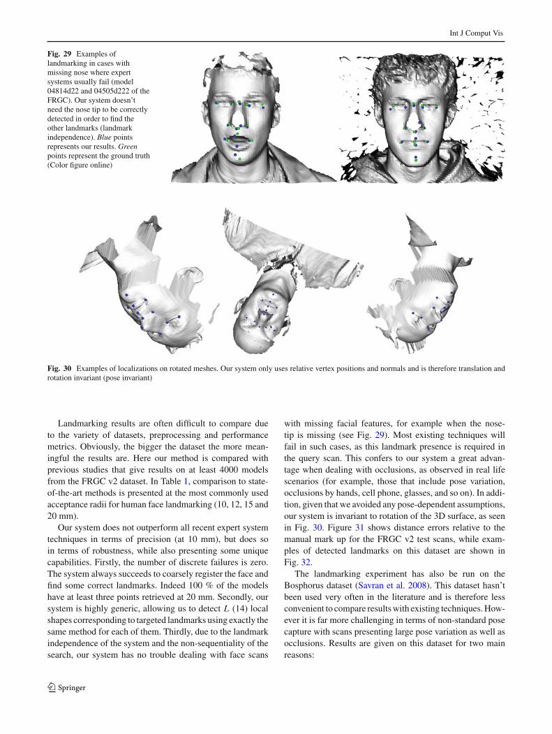
Int J Comput Vis
Fig. 29 Examples oflandmarking in cases withmissing nose where expertsystems usually fail (model04814d22 and 04505d222 of theFRGC). Our system doesn’tneed the nose tip to be correctlydetected in order to find theother landmarks (landmarkindependence). Blue pointsrepresents our results. Greenpoints represent the ground truth(Color figure online)
Fig. 30 Examples of localizations on rotated meshes. Our system only uses relative vertex positions and normals and is therefore translation androtation invariant (pose invariant)
Landmarking results are often difficult to compare dueto the variety of datasets, preprocessing and performancemetrics. Obviously, the bigger the dataset the more mean-ingful the results are. Here our method is compared withprevious studies that give results on at least 4000 modelsfrom the FRGC v2 dataset. In Table 1, comparison to state-of-the-art methods is presented at the most commonly usedacceptance radii for human face landmarking (10, 12, 15 and20 mm).
Our system does not outperform all recent expert systemtechniques in terms of precision (at 10 mm), but does soin terms of robustness, while also presenting some uniquecapabilities. Firstly, the number of discrete failures is zero.The system always succeeds to coarsely register the face andfind some correct landmarks. Indeed 100 % of the modelshave at least three points retrieved at 20 mm. Secondly, oursystem is highly generic, allowing us to detect L (14) localshapes corresponding to targeted landmarks using exactly thesame method for each of them. Thirdly, due to the landmarkindependence of the system and the non-sequentiality of thesearch, our system has no trouble dealing with face scans
with missing facial features, for example when the nose-tip is missing (see Fig. 29). Most existing techniques willfail in such cases, as this landmark presence is required inthe query scan. This confers to our system a great advan-tage when dealing with occlusions, as observed in real lifescenarios (for example, those that include pose variation,occlusions by hands, cell phone, glasses, and so on). In addi-tion, given that we avoided any pose-dependent assumptions,our system is invariant to rotation of the 3D surface, as seenin Fig. 30. Figure 31 shows distance errors relative to themanual mark up for the FRGC v2 test scans, while exam-ples of detected landmarks on this dataset are shown inFig. 32.
The landmarking experiment has also be run on theBosphorus dataset (Savran et al. 2008). This dataset hasn’tbeen used very often in the literature and is therefore lessconvenient to compare results with existing techniques. How-ever it is far more challenging in terms of non-standard posecapture with scans presenting large pose variation as well asocclusions. Results are given on this dataset for two mainreasons:
123

Int J Comput Vis
Fig. 31 Distance error for the 14 landmarks. The candle stick repre-sents the min/Q1/median/Q3/max values. The plus sign represents themean
– to highlight some limitations of our technique that couldnot have been detected with the FRGC dataset alone;
– to provide enough data to allow results comparison withthis dataset in future research.
Table 2 contains the landmark retrieval rates for the dif-ferent parts of the dataset, as well as for the whole set. Scans
of yaw rotation marked as 90◦ were not used due to theirpoor associated descriptor maps (higher resolution might benecessary to treat those cases). Moreover, scans marked asIGN (ignored) in the dataset have also been discarded. Intotal we tested 4,339 face scans from the Bosphorus dataset.Figure 33 shows examples of landmark localization on someof these scans.
6.3.1 Limitations
A limitation of our system is that it relies heavily on localdescriptors. Therefore, the robustness of the system stronglydepends on the robustness of the local descriptors used. Ifthose are not robust to occlusion the local DL-scores mightbe spurious and detection quality will suffer. For exam-ple, in a profile view, when a vertex is near the borderof the mesh, its local neighborhood is incomplete and thedescriptors computed on this neighborhood are likely to benoisy. It might be interesting to develop different special-ized descriptors that can detect keypoints near the borderof the mesh using, for example, extracted 2D curves along
Table 2 Results on the more challenging Bosphorus dataset using our landmarking method
The training set is composed of 99 faces from the neutral subset of the dataset. The results are provided for the four most commonly used acceptanceradii in landmarking to facilitate future results comparison
123

Int J Comput Vis
Fig. 32 Examples oflandmarks detected by oursystem. Landmarks are definedby the positions of ascale-adapted landmark model,L, which is a set of L (position,label pairs) for an average facemesh. The model L is equippedwith a triangulation (i.e. it isdisplayed as a graph) purely toaid visualization. The input facemeshes are taken from theFRGC v2 dataset
the direction of occlusion. Combining the DL-scores usingthese new descriptors can easily be done within our frame-work.
In Fig. 34, the worst case landmark localizations in termsof the three global registration metrics are presented for the
FRGC test set. When registering the ground-truth and thelocalized landmarks, the transformation is decomposed bysteps into a mean translation (aligning the centroids), a scalechange (by scaling the mean edge length) and a final rota-tion, when translation has been canceled and scale equalized.
123
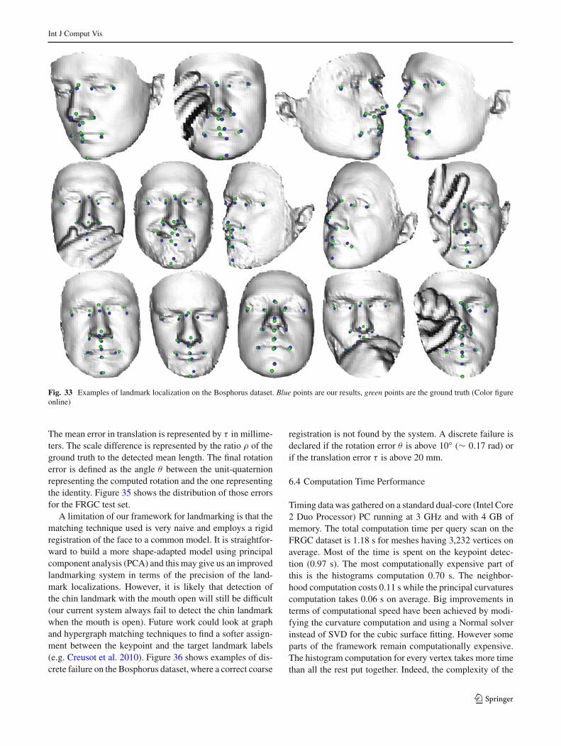
Int J Comput Vis
Fig. 33 Examples of landmark localization on the Bosphorus dataset. Blue points are our results, green points are the ground truth (Color figureonline)
The mean error in translation is represented by τ in millime-ters. The scale difference is represented by the ratio ρ of theground truth to the detected mean length. The final rotationerror is defined as the angle θ between the unit-quaternionrepresenting the computed rotation and the one representingthe identity. Figure 35 shows the distribution of those errorsfor the FRGC test set.
A limitation of our framework for landmarking is that thematching technique used is very naive and employs a rigidregistration of the face to a common model. It is straightfor-ward to build a more shape-adapted model using principalcomponent analysis (PCA) and this may give us an improvedlandmarking system in terms of the precision of the land-mark localizations. However, it is likely that detection ofthe chin landmark with the mouth open will still be difficult(our current system always fail to detect the chin landmarkwhen the mouth is open). Future work could look at graphand hypergraph matching techniques to find a softer assign-ment between the keypoint and the target landmark labels(e.g. Creusot et al. 2010). Figure 36 shows examples of dis-crete failure on the Bosphorus dataset, where a correct coarse
registration is not found by the system. A discrete failure isdeclared if the rotation error θ is above 10◦ (∼ 0.17 rad) orif the translation error τ is above 20 mm.
6.4 Computation Time Performance
Timing data was gathered on a standard dual-core (Intel Core2 Duo Processor) PC running at 3 GHz and with 4 GB ofmemory. The total computation time per query scan on theFRGC dataset is 1.18 s for meshes having 3,232 vertices onaverage. Most of the time is spent on the keypoint detec-tion (0.97 s). The most computationally expensive part ofthis is the histograms computation 0.70 s. The neighbor-hood computation costs 0.11 s while the principal curvaturescomputation takes 0.06 s on average. Big improvements interms of computational speed have been achieved by modi-fying the curvature computation and using a Normal solverinstead of SVD for the cubic surface fitting. However someparts of the framework remain computationally expensive.The histogram computation for every vertex takes more timethan all the rest put together. Indeed, the complexity of the
123

Int J Comput Vis
Fig. 34 Four worst cases in the FRGC test set by global registration metric: largest angle, smallest scale ratio, largest scale ratio, largest meantranslation
Fig. 35 Distribution of the global registration errors on the FRGC test set
Fig. 36 Examples of discrete failures on the Bosphorus dataset. The 17 failures detected on the 4,339 scans (0.39 %) are mainly due to occlusion(7 scans) and rotation (six ‘yaw’ and one ‘pitch’ scans). The three remaining failures are on scans that show exaggerated facial expressions
naive algorithm used to get the histograms is quadratic inthe number of vertices. The speed can be improved by usingbetter structures for locality retrieval, for example an octreestructure. The computation of DL-score and landmark scoremaps is performed under 0.03 s. The final matching usingRANSAC takes 0.18 s with 130 landmark candidates perface on average.
The total computation time per input scan on the Bospho-rus dataset was 0.55 s for meshes having 1,879 vertices onaverage.
7 Conclusions
A simple method has been proposed to deal with keypointdetection and landmarking of learned local shapes. Thismethod requires landmarks on training meshes to be man-ually marked up with a set of landmarks defined in a land-mark model. One can think of this landmark model as beingaugmented by learned keypoint detector functions, fλ, (oneper landmark), and this can then be used to automaticallylandmark unseen query meshes.
123

Int J Comput Vis
A flexible aspect of our method is that it doesn’t assumethat detected points on the mesh should have an extremalvalue over a descriptor map. Instead, it assumes that thematching score of this descriptor against a learned distrib-ution should be maximal.
While other techniques are landmark-dependent, our canbe be applied to any shape of interest as long as trainingis provided. The same method is used to detect the nose,an eye’s corner or the chin. We detected 14 facial features,while expert system methods are usually limited to a fewsalient features (see Table 1).
While being more fuzzy (many-valued) compared toexpert system methods, we believe that this kind of approachis necessary to deal with uncontrolled input data. In particu-lar, it is more likely to be successful for non-cooperative facepreprocessing where there are great uncertainties about whatis present in the query scan.
In our opinion, the main gain in performance in the futurewill come from adding new local descriptors that better dealwith occlusions and profile views, leading to less ambiguouskeypoints. Local refinement of coarse landmark localizationwill also be essential to gain precision and high retrieval ratesat low acceptance radii.
References
Alyuz, N., Gokberk, B., & Akarun, L. (2010). Regional registrationfor expression resistant 3-d face recognition. IEEE Transactionson Information Forensics and Security, 5(3), 425–440. doi:10.1109/TIFS.2010.2054081.
Ben Azouz, Z., Shu, C., & Mantel, A. (2006). Automatic locating ofanthropometric landmarks on 3d human models. In Third interna-tional symposium on 3D data processing, visualization, and trans-mission (pp. 750–757, 14–16). doi:10.1109/3DPVT.2006.34.
Berretti, S., Bimbo, A. D., & Pala, P. (2010). Recognition of 3d faceswith missing parts based on profile networks. 1st ACM workshopon 3D object. Retrieval (ACM 3DOR’10) (pp. 81–86). doi:10.1145/1877808.1877825.
Besl, P., & McKay, N. (1992). A method for registration of 3d shapes.IEEE Transactions on Pattern Analysis and Machine Intelligence,14(2), 239–256. doi:10.1109/34.121791.
Boyer, E., Bronstein, A. M., Bronstein, M. M., Bustos4, B., Darom,T., Horaud, R., et al.. (2011). Shrec 2011: robust feature detectionand description benchmark. Eurographics workshop on 3D object.Retrieved. doi:10.2312/3DOR/3DOR11/071-078.
Castellani, U., Cristani, M., Fantoni, S., & Murino, V. (2008). Sparsepoints matching by combining 3d mesh saliency with statisticaldescriptors. Computer Graphics Forum, 27(2), 643–652. doi:10.1111/j.1467-8659.2008.01162.x.
Chang, K. I., Bowyer, K., & Flynn, P. (2006). Multiple nose regionmatching for 3d face recognition under varying facial expression.IEEE Transactions on Pattern Analysis and Machine Intelligence,28(10), 1695–1700. doi:10.1109/TPAMI.2006.210.
Choi, E., & Lee, C. (2003). Feature extraction based on the bhat-tacharyya distance. Pattern Recognition, 36(8), 1703–1709. doi:10.1016/S0031-3203(03)00035-9.
Colbry, D., Stockman, G., & Jain, A. (2005). Detection of anchor pointsfor 3d face verification. In IEEE computer society conference on
computer vision and pattern recognition—workshops, 2005. CVPRworkshops (pp. 118–118, 25–25). doi:10.1109/CVPR.2005.441.
Creusot, C. (2011). Automatic landmarking for non-cooperative 3Dface recognition. Ph.D. thesis, University of York. http://etheses.whiterose.ac.uk/2274/.
Creusot, C., Pears, N., & Austin, J. (2010). 3D face landmark labelling.In Proceedings of the ACM workshop on 3D object retrieval. ACM,3DOR ’10 (pp. 27–32). doi:10.1145/1877808.1877815.
Creusot, C., Pears, N., & Austin, J. (2011). Automatic keypointdetection on 3d faces using a dictionary of local shapes. In 2011International conference on 3D imaging, modeling, processing, visu-alization and transmission (3DIMPVT) (pp. 204–211). doi:10.1109/3DIMPVT.2011.33.
D’Hose, J., Colineau, J., Bichon, C., & Dorizzi, B. (2007). Preciselocalization of landmarks on 3d faces using gabor wavelets. In FirstIEEE international conference on biometrics: theory, applications,and systems, 2007. BTAS 2007 (pp. 1–6). doi:10.1109/BTAS.2007.4401927.
Dibeklioglu, H., Salah, A., & Akarun, L. (2008). 3d facial landmarkingunder expression, pose, and occlusion variations. In BTAS08 (pp.1–6). doi:10.1109/BTAS.2008.4699324.
Faltemier, T., Bowyer, K., & Flynn, P. (2008). Rotated profile signaturesfor robust 3d feature detection. In 8th IEEE international conferenceon automatic face gesture Recognition, 2008. FG ’08 (pp. 1–7, 17–19). doi:10.1109/AFGR.2008.4813413.
Fischler, M. A., & Bolles, R. C. (1981). Random sample consensus: aparadigm for model fitting with applications to image analysis andautomated cartography. Communications of the ACM, 24(6), 381–395. doi:10.1145/358669.358692.
Freund, Y., & Schapire, R. E. (1997). A decision-theoretic general-ization of on-line learning and an application to boosting. Journalof Computer and System Sciences, 55, 119–139. doi:10.1006/jcss.1997.1504.
Goldfeather, J., & Interrante, V. (2004) A novel cubic-order algorithmfor approximating principal direction vectors. ACM Transactions onGraphics, 23(1), 45–63. doi:10.1145/966131.966134.
Itskovich, A., & Tal, A. (2011). Surface partial matching and applica-tion to archaeology. Computers & Graphics, 35(2), 334–341. doi:10.1016/j.cag.2010.11.010.
Johnson, A., & Hebert, M. (1999). Using spin images for efficient objectrecognition in cluttered 3d scenes. IEEE Transactions on PatternAnalysis and Machine Intelligence, 21(1), 433–449.
Kim, J.-S., & Choi, S.-M. (2009). Symmetric deformation of 3d facescans using facial features and curvatures. Computer Animation andVirtual Worlds, 20, 289–300. doi:10.1002/cav.v20:2/3.
Lowe, D. G., (2004). Distinctive image features from scale-invariantkeypoints. International Journal of Computer Vision, 60(2), 91–110.doi:10.1023/B:VISI.0000029664.99615.94.
Max, N. (1999). Weights for computing vertex normals from facetnormals. Journal of Graphics Tools, 4, 1–6. http://portal.acm.org/citation.cfm?id=334709.334710.
Mayo, M., & Zhang, E. (2009). 3D face recognition using multi-view keypoint matching. Sixth IEEE International Conference onAdvanced Video and Signal Based Surveillance, 2009. AVSS ’09 (pp.290–295). doi:10.1109/AVSS.2009.11.
Mian, A., Bennamoun, M., & Owens, R. (2010). On the repeatabilityand quality of keypoints for local feature-based 3d object retrievalfrom cluttered scenes. International Journal of Computer Vision,89(2), 348–361. doi:10.1007/s11263-009-0296-z.
Mian, A. S., Bennamoun, M., & Owens, R. (2008). Keypoint detec-tion and local feature matching for textured 3d face recognition.International Journal of Computer Vision, 79(1), 1–12. doi:10.1007/s11263-007-0085-5.
Mian, A. S., Bennamoun, M., & Owens, R. A. (2006). Automatic 3dface detection, normalization and recognition. In 3DPVT (pp. 735–742). doi:10.1109/3DPVT.2006.32.
123

Int J Comput Vis
Pears, N., Heseltine, T., & Romero, M., (2010). From 3D point cloudsto pose-normalised depth maps. International Journal of ComputerVision, 89(2), 152–176. doi:10.1007/s11263-009-0297-y.
Phillips, P., Flynn, P., Scruggs, T., Bowyer, K., Chang, J., Hoffman, K.,et al. (2005). Overview of the face recognition grand challenge. InIEEE computer society conference on computer vision and patternrecognition, 2005. CVPR 2005 (Vol. 1, pp. 947–954). doi:10.1109/CVPR.2005.268.
Romero, M., & Pears, N., (2009). Landmark localisation in 3d facedata. In Sixth IEEE international conference on advanced video andsignal based surveillance, 2009. AVSS ’09 (pp. 73–78). doi:10.1109/AVSS.2009.90.
Romero-Huertas, M., & Pears, N. (2008). 3D facial landmark locali-sation by matching simple descriptors. In 2nd IEEE internationalconference on biometrics: theory, applications and systems, BTAS2008 (pp. 1–6). doi:10.1109/BTAS.2008.4699390.
Rubner, Y., Tomasi, C., & Guibas, L. J. (2000). The earth mover’sdistance as a metric for image retrieval. International Journal ofComputer Vision, 40, 99–121. doi:10.1023/A:1026543900054.
Savran, A., Alyüz, N., Dibeklioglu, H., Çeliktutan, O., Gökberk, B.,Sankur, B., et al. (2008). Bosphorus database for 3d face analysis.In Biometrics and identity management: first European workshop,BIOID 2008 (pp. 47–56). Springer: Roskilde, Denmark. doi:10.1007/978-3-540-89991-4_6.
Segundo, M., Queirolo, C., Bellon, O., & Silva, L., (2007). Automatic3D facial segmentation and landmark detection. In 14th Internationalconference on image analysis and processing, 2007 (ICIAP 2007)(pp. 431–436). doi:10.1109/ICIAP.2007.4362816.
Segundo M., Silva L., Bellon O. R. P., & Queirolo C. C., (2010).Automatic face segmentation and facial landmark detection in rangeimages. IEEE Transactions on Systems, Man, and Cybernetics,Part B: Cybernetics, 40(5), 1319–1330. doi:10.1109/TSMCB.2009.2038233.
Shotton, J., Johnson, M., & Cipolla, R., (2008). Semantic texton forestsfor image categorization and segmentation. IEEE Computer SocietyConference on Computer Vision and Pattern Recognition (pp. 1–8).doi:10.1109/CVPR.2008.4587503.
Szeptycki, P., Ardabilian, M., & Chen, L., (2009). A coarse-to-fine cur-vature analysis-based rotation invariant 3D face landmarking. Inter-national conference on biometrics: theory, applications and systems(pp. 32–37). doi:10.1109/BTAS.2009.5339052.
Viola, P., & Jones, M. J. (2004). Robust real-time face detection. Inter-national Journal of Computer Vision, 57, 137–154. doi:10.1023/B:VISI.0000013087.49260.fb.
Zaharescu, A., Boyer, E., Varanasi, K., & Horaud, R., (2009). Surfacefeature detection and description with applications to mesh match-ing. IEEE Conference on Computer Vision and Pattern Recognition(CVPR), San Francisco (pp. 373–380). doi:10.1109/CVPR.2009.5206748.
Zhao X., Dellandr anda E., Chen L., & Kakadiaris I. A. (2011). Accu-rate landmarking of three-dimensional facial data in the presence offacial expressions and occlusions using a three-dimensional statisti-cal facial feature model. IEEE Transactions on Systems, Man, andCybernetics, Part B: Cybernetics, 41(5), 1417–1428. doi:10.1109/TSMCB.2011.2148711.
123