energies

Article

A Marine Gas Turbine Fault Diagnosis Method Basedon Endogenous Irreversible Loss

Yunpeng Cao * , Junqi Luan, Guodong Han, Xinran Lv and Shuying Li

College of Power and Energy Engineering, Harbin Engineering University, Harbin 150001, China;luanjunqi@hrbeu.edu.cn (J.L.); hanguodong@hrbeu.edu.cn (G.H.); 13664504988@hrbeu.edu.cn (X.L.);lishuying@hrbeu.edu.cn (S.L.)* Correspondence: caoyunpeng@hrbeu.edu.cn

Received: 31 October 2019; Accepted: 4 December 2019; Published: 9 December 2019�����������������

Abstract: When a malfunction occurs in a marine gas turbine, its thermal efficiency will decreaseslightly, and the gas path fault is often difficult to distinguish. In order to solve this problem, based onthe second law of thermodynamics, the endogenous irreversible loss (EIL) model of the marine gasturbine is established, and the exergy loss analysis under normal conditions is carried out to verifythe accuracy of the model. The fault diagnosis of gas turbine gas path based on EIL is proposed,and a simulation experiment conducted on a three-shaft marine gas turbine demonstrated thatthe proposed approach can detect and isolate gas path fault accurately under different operatingconditons and enviroments.

Keywords: gas turbine; gas path; fault diagnosis; endogenous irreversible loss

1. Introduction

A gas turbine is a complex thermal system. Its operation process is a cross-coupled thermodynamicprocess. When a certain component fails, it often causes the performance degradation of the entireequipment and even catastrophic consequences. The high-speed airflow passage composed of severalcomponents of the gas turbine is collectively referred to as the gas path. Since the turbine is required toinhale a large amount of air during operation, the air often contains salt ingested particles, moisture,and other corrosive substances, which may cause damage to the interior of the turbine. These gaspath components are subject to wear, corrosion, fouling, and other external damage, which in turncauses the performance of the gas turbine to decrease [1,2]. Therefore, it is necessary to find a way toaccurately monitor the gas path failure.

In recent years, many gas path fault diagnosis methods have been proposed to assess gasturbine health status, such as nonlinear gas path analysis [3–5], rule-based fuzzy expert system [6,7],Bayesian hierarchical models [8,9], neural networks [10–12], genetic algorithm [13,14], multiple-modelmethod [15,16], and exergy analysis [17]. Gas path analysis is an inversely mathematical problemto obtain the deviation of component performance parameters over gas path measured variables.Most case studies show that artificial intelligence methods, such as artificial neural networks, Bayesianhierarchical models, and fuzzy expert systems, may effectively isolate the faulty components but noteasily assess the severity of the fault [18].

The model-based approach is an analytical redundancy approach that diagnoses the fault basedon the residual signal between the measurements and the gas turbine’s mathematical model. Kalmanfilter is a typical model-based approach and is widely used in gas path fault diagnosis [18]. However,model-based approaches require accurate gas turbine mathematical models, and their reliabilitydecreases as system complexity increases. Meanwhile, when a gas path fault occurs, the parameterchange may be extremely weak and difficult to monitor.

Energies 2019, 12, 4677; doi:10.3390/en12244677 www.mdpi.com/journal/energies

Energies 2019, 12, 4677 2 of 18

It is a new idea and direction to diagnose the gas path of gas turbine based on the exergyloss [19–25]. According to the second law of thermodynamics, we know that the exergy efficiency isan important indicator to measure the irreversibility of the work of the thermal system. The exergyloss is an actual loss in the process of energy conversion. Therefore, it is more suitable to describe thefunction of a thermal system. And when the fault occurs, the change of the exergy loss is greater thanthe rest of the thermal parameters, which can improve the sensitivity of the diagnosis. In recent years,on the basis of exergy research, some scholars have proposed the concept of thermoeconomic [26–29],not only based on the second law of thermodynamics, but also introduced the basic ideas of systemengineering, optimization theory, and decision theory, capable of analyzing complex energy systems.

When a gas turbine fault occurs, the exergy loss of the gas turbine is divided into exogenousirreversible loss and endogenous irreversible loss (EIL) [30–32]—where the EIL can better characterizethe impact of the gas turbine component itself, and the complicated coupling relationship of gasturbines and the EIL of internal sources may also change when other components fail. Therefore,the use of the EIL for fault diagnosis is the key research content of this paper.

At present, most of the fault diagnosis based on the exergy balance analysis principle of gasturbines is on industrial single-shaft or two-shaft gas turbines, while there are few studies on marinethree-shaft gas turbines. Furthermore, the coupling relationship of the three-shaft marine gas turbineis more complicated. The operating environment of the marine gas turbine is more complicated andharsh than the industrial gas turbine, and the operating conditions are more variable. A new faultdiagnosis method suitable for the marine three-shaft gas turbine is urgently needed.

In this regard, we have conducted the following research. In Section 2, the EIL models of themarine gas turbine under healthy and faulty are established. In Section 3, the diagnosis process basedon the EIL is established. In Section 4, taking marine three-shaft gas turbine as the object, a faultdiagnosis algorithm based on EIL is proposed, which is used for the verification of the algorithm underthe condition of typical gas path fault.

2. EIL Model of Gas Turbine

Slight changes in performance parameters may cause changes in multiple thermal parametersof marine gas turbines under different operating conditions. Slight changes in thermal parametersare difficult to identify, causing problems with diagnostic difficulties. On the basis of the second lawof thermodynamics, the use of exergy balance has better sensitivity for fault diagnosis of marine gasturbine gas paths.

This section introduces the exergy balance analysis method and establishes its physical structureand productive structure by analyzing the working principle of the marine gas turbine. Then, based onthe nonlinear model of the marine gas turbine [33], the EIL model of marine gas turbine is established.

2.1. EIL Analysis of Gas Turbine

The exergy analysis method is based on the second law of thermodynamics, which provide amethod to measure the actual performance and identify the causes of thermodynamic losses. Since theenergy of different forms has mutual conservation of mass and qualitative difference, the two propertiesare different. As a physical quantity for evaluating energy value, exergy is a physical quantity thatreflects both the “mass” and “quantity” of energy. In various forms of energy, such as mechanicalenergy, electrical energy, etc. which can all be converted into heat energy, the theoretical conversionefficiency is close to 100%, and this kind of energy that can be converted infinitely is called exergy,which is recorded as B.

Exergy loss occurs in any actual process, that is, a portion of the fuel exergy is lost during theproduction process. Using the definition of fuel and product, the process component exergy balancecan be expressed as:

F = P + I (1)

Energies 2019, 12, 4677 3 of 18

where F represents the component fuel, P which represents the component product, and I representsthe loss of exergy of the component.

Therefore, fuel consumption is also related to the EIL of the process (exergy loss), which can becharacterized by the unit consumption k.

k = F/P (2)

When a gas path fault occurs in a marine gas turbine, the exergy must change. The changedpart is composed of endogenous irreversible loss (EIL) and exogenous irreversible loss. The EIL cancharacterize the impact of fault for the marine gas turbine unit itself better. At the same time, due tothe complex coupling relationship of the gas turbine, the EIL may also change greatly when othercomponents fail. Compared with the other thermodynamic parameters for fault diagnosis, the EIL forfault diagnosis increases its sensitivity, and the number of parameters used is reduced, which simplifiesthe complexity of diagnosis. Thus, it is a new research direction.

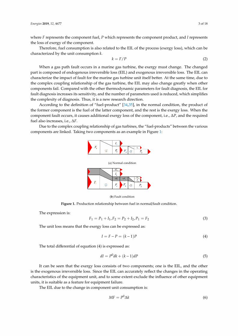
According to the definition of “fuel-product” [34,35], in the normal condition, the product ofthe former component is the fuel of the latter component, and the rest is the exergy loss. When thecomponent fault occurs, it causes additional exergy loss of the component, i.e., ∆P, and the requiredfuel also increases, i.e., ∆F.

Due to the complex coupling relationship of gas turbines, the “fuel-products” between the variouscomponents are linked. Taking two components as an example in Figure 1:

Energies 2019, 12, x 3 of 19

where F represents the component fuel, P which represents the component product, and I represents the loss of exergy of the component.

Therefore, fuel consumption is also related to the EIL of the process (exergy loss), which can be characterized by the unit consumption k.

k F P= (2)

When a gas path fault occurs in a marine gas turbine, the exergy must change. The changed part is composed of endogenous irreversible loss (EIL) and exogenous irreversible loss. The EIL can characterize the impact of fault for the marine gas turbine unit itself better. At the same time, due to the complex coupling relationship of the gas turbine, the EIL may also change greatly when other components fail. Compared with the other thermodynamic parameters for fault diagnosis, the EIL for fault diagnosis increases its sensitivity, and the number of parameters used is reduced, which simplifies the complexity of diagnosis. Thus, it is a new research direction.

According to the definition of “fuel-product” [34,35], in the normal condition, the product of the former component is the fuel of the latter component, and the rest is the exergy loss. When the component fault occurs, it causes additional exergy loss of the component, i.e., ΔP, and the required fuel also increases, i.e., ΔF.

Due to the complex coupling relationship of gas turbines, the “fuel-products” between the various components are linked. Taking two components as an example in Figure 1:

(a) Normal condition

(b) Fault condition

Figure 1. Production relationship between fuel in normal/fault condition.

The expression is:

= +1 1 1F P I , = +2 2 2F P I , =1 2P F (3)

The unit loss means that the exergy loss can be expressed as:

= − = −( 1)I F P k P (4)

The total differential of equation (4) is expressed as:

= + −0 ( 1)dI P dk k dP (5)

It can be seen that the exergy loss consists of two components; one is the EIL, and the other is the exogenous irreversible loss. Since the EIL can accurately reflect the changes in the operating characteristics of the equipment unit, and to some extent exclude the influence of other equipment units, it is suitable as a feature for equipment failure.

The EIL due to the change in component unit consumption is:

= Δ0MF P k (6)

Figure 1. Production relationship between fuel in normal/fault condition.

The expression is:F1 = P1 + I1, F2 = P2 + I2, P1 = F2 (3)

The unit loss means that the exergy loss can be expressed as:

I = F− P = (k− 1)P (4)

The total differential of equation (4) is expressed as:

dI = P0dk + (k− 1)dP (5)

It can be seen that the exergy loss consists of two components; one is the EIL, and the otheris the exogenous irreversible loss. Since the EIL can accurately reflect the changes in the operatingcharacteristics of the equipment unit, and to some extent exclude the influence of other equipmentunits, it is suitable as a feature for equipment failure.

The EIL due to the change in component unit consumption is:

MF = P0∆k (6)

Energies 2019, 12, 4677 4 of 18

2.2. Physical Structure and Productive Structure of the Marine Gas Turbine

In order to exergy balance analysis, a marine gas turbine is divided into several components orprocess components. A process component is a functional component that has a production purposecorresponding to a real device. However, the process component is not necessarily a specific physicalstructure device, and different devices can be combined into one process component, or one physicalstructure device can be further decomposed into several process components.

The productive structure model is to facilitate the analysis of the physical structure of the systemand the depreciation of each flow. The structural characteristics of the marine gas turbine wereanalyzed in Figure 2. It can be seen that the air (0) is compressed by the low-pressure compressor(LC) to generate the low-pressure air (1) and then continues to be compressed by the high-pressurecompressor (HC) to generate high-pressure air (2). The high-pressure air (2) and the fuel (10) are fullymixed and burned in the combustion chamber (CC) to form high temperature and high-pressure gas(3). The gas (3) enters the high-pressure turbine to expand to do work, the generated energy (8) drivesthe high-pressure compressor to rotate, and the expanded gas (4) enters the low-pressure turbine(LC) for further expansion, the energy (9) generated by low-pressure turbine drives the low-pressurecompressor to rotate. Finally, the expanded gas (5) enters the power turbine (PT) to continue to expandto do work, the generated energy (6) drives the generator(G) to generate electricity (7), and the exhaust(11) is discharged into the atmosphere. According to the energy flow and mass flow described inFigure 2, the physical structure of the gas turbine is shown in Figure 3.

Energies 2019, 12, x 4 of 19

2.2. Physical Structure and Productive Structure of the Marine Gas Turbine

In order to exergy balance analysis, a marine gas turbine is divided into several components or process components. A process component is a functional component that has a production purpose corresponding to a real device. However, the process component is not necessarily a specific physical structure device, and different devices can be combined into one process component, or one physical structure device can be further decomposed into several process components.

The productive structure model is to facilitate the analysis of the physical structure of the system and the depreciation of each flow. The structural characteristics of the marine gas turbine were analyzed in Figure 2. It can be seen that the air (0) is compressed by the low-pressure compressor (LC) to generate the low-pressure air (1) and then continues to be compressed by the high-pressure compressor (HC) to generate high-pressure air (2). The high-pressure air (2) and the fuel (10) are fully mixed and burned in the combustion chamber (CC) to form high temperature and high-pressure gas (3). The gas (3) enters the high-pressure turbine to expand to do work, the generated energy (8) drives the high-pressure compressor to rotate, and the expanded gas (4) enters the low-pressure turbine (LC) for further expansion, the energy (9) generated by low-pressure turbine drives the low-pressure compressor to rotate. Finally, the expanded gas (5) enters the power turbine (PT) to continue to expand to do work, the generated energy (6) drives the generator(G) to generate electricity (7), and the exhaust (11) is discharged into the atmosphere. According to the energy flow and mass flow described in Figure 2, the physical structure of the gas turbine is shown in Figure 3.

As can be seen from Figure 3, the marine gas turbine is divided into six components: The low-pressure compressor, the high-pressure compressor, the combustor, the high-pressure turbine, the low-pressure turbine, and the power turbine. The generator connected to the power turbine belongs to the gas turbine. The process of physical flow is shown by the arrow, and there are 11 physical flows between components and the environment.

Figure 2. The layout of a marine three-shaft gas turbine.

Figure 3. The physical structure of the marine three-shaft gas turbine.

From the physical structure, we can establish the productive structure of the marine gas turbine, as shown in Figure 4. There are two fuels in the low-pressure compressor, one is F1 which is supplied by the product P5 that is produced by the low-pressure turbine, and the other is flow 0, and its exergy

Figure 2. The layout of a marine three-shaft gas turbine.

Energies 2019, 12, x 4 of 19

2.2. Physical Structure and Productive Structure of the Marine Gas Turbine

In order to exergy balance analysis, a marine gas turbine is divided into several components or process components. A process component is a functional component that has a production purpose corresponding to a real device. However, the process component is not necessarily a specific physical structure device, and different devices can be combined into one process component, or one physical structure device can be further decomposed into several process components.

The productive structure model is to facilitate the analysis of the physical structure of the system and the depreciation of each flow. The structural characteristics of the marine gas turbine were analyzed in Figure 2. It can be seen that the air (0) is compressed by the low-pressure compressor (LC) to generate the low-pressure air (1) and then continues to be compressed by the high-pressure compressor (HC) to generate high-pressure air (2). The high-pressure air (2) and the fuel (10) are fully mixed and burned in the combustion chamber (CC) to form high temperature and high-pressure gas (3). The gas (3) enters the high-pressure turbine to expand to do work, the generated energy (8) drives the high-pressure compressor to rotate, and the expanded gas (4) enters the low-pressure turbine (LC) for further expansion, the energy (9) generated by low-pressure turbine drives the low-pressure compressor to rotate. Finally, the expanded gas (5) enters the power turbine (PT) to continue to expand to do work, the generated energy (6) drives the generator(G) to generate electricity (7), and the exhaust (11) is discharged into the atmosphere. According to the energy flow and mass flow described in Figure 2, the physical structure of the gas turbine is shown in Figure 3.

As can be seen from Figure 3, the marine gas turbine is divided into six components: The low-pressure compressor, the high-pressure compressor, the combustor, the high-pressure turbine, the low-pressure turbine, and the power turbine. The generator connected to the power turbine belongs to the gas turbine. The process of physical flow is shown by the arrow, and there are 11 physical flows between components and the environment.

Figure 2. The layout of a marine three-shaft gas turbine.

Figure 3. The physical structure of the marine three-shaft gas turbine.

From the physical structure, we can establish the productive structure of the marine gas turbine, as shown in Figure 4. There are two fuels in the low-pressure compressor, one is F1 which is supplied by the product P5 that is produced by the low-pressure turbine, and the other is flow 0, and its exergy

Figure 3. The physical structure of the marine three-shaft gas turbine.

As can be seen from Figure 3, the marine gas turbine is divided into six components:The low-pressure compressor, the high-pressure compressor, the combustor, the high-pressure turbine,the low-pressure turbine, and the power turbine. The generator connected to the power turbine belongsto the gas turbine. The process of physical flow is shown by the arrow, and there are 11 physical flowsbetween components and the environment.

From the physical structure, we can establish the productive structure of the marine gas turbine,as shown in Figure 4. There are two fuels in the low-pressure compressor, one is F1 which is suppliedby the product P5 that is produced by the low-pressure turbine, and the other is flow 0, and itsexergy is equal to 0. The product of the low-pressure compressor is exergy flow P1. The fuel F2 of thehigh-pressure compressor comes from the product of high-pressure turbine P4, and its product is exergyflow P2. The fuel of the combustor is fossil fuel F3, and its product is P3. We can see from Figure 3,the expansion gas is not fully expanded in the high-pressure turbine; it also enters low-pressure turbineand the power turbine to continue to expand, so a junction point “J” to present the sum of useful

Energies 2019, 12, 4677 5 of 18

product P1, P2, and P3, and a breakpoint “B” to present the relationship that product divided into threefuel flows, F4 enters into high-pressure turbine, F5 enters into low-pressure turbine, and F6 entersinto power turbine. P6 is the product of the power turbine and is also the fuel of generator. It can beseen from Figure 4, the productive structure indicates a detailed analysis of the “production” and“consumption” processes of the marine gas turbine.

Energies 2019, 12, x 5 of 19

is equal to 0. The product of the low-pressure compressor is exergy flow P1. The fuel F2 of the high-pressure compressor comes from the product of high-pressure turbine P4, and its product is exergy flow P2. The fuel of the combustor is fossil fuel F3, and its product is P3. We can see from Figure 3, the expansion gas is not fully expanded in the high-pressure turbine; it also enters low-pressure turbine and the power turbine to continue to expand, so a junction point “J” to present the sum of useful product P1, P2, and P3, and a breakpoint “B” to present the relationship that product divided into three fuel flows, F4 enters into high-pressure turbine, F5 enters into low-pressure turbine, and F6 enters into power turbine. P6 is the product of the power turbine and is also the fuel of generator. It can be seen from Figure 4, the productive structure indicates a detailed analysis of the “production” and “consumption” processes of the marine gas turbine.

Figure 4. Productive structure of the marine three-shaft gas turbine.

2.3. EIL Model of Components

The establishment of the productive structure makes the resource allocation of the marine gas turbine represented graphically. According to the productive structure, the “fuel” and “product” of each process component were analyzed. The EIL model of the marine gas turbine can be established according to the productive structure.

2.3.1. EIL Model of Compressors

The compressor is one of the main components of the gas turbine, which uses the mechanical energy supplied by the low-pressure turbine to continuously compress and deliver the gas. For compressor simulation modeling, compressor characteristics are particularly important. It is necessary to obtain the flow and efficiency by converting the speed and pressure ratio. The enthalpy and entropy of equipment inlet and outlet are functions of temperature, which can be obtained by fitting equation, so as to calculate the exergy of equipment inlet and outlet.

The calculation equation of the EIL of the low-pressure compressor is:

= −'

1 11 1 '

11

( )F F

M F PPP

(7)

= − − −1 1 0 0 1 0( )P h h T s s (8)

ω= 21

12 LCLTF J (9)

Figure 4. Productive structure of the marine three-shaft gas turbine.

2.3. EIL Model of Components

The establishment of the productive structure makes the resource allocation of the marine gasturbine represented graphically. According to the productive structure, the “fuel” and “product” ofeach process component were analyzed. The EIL model of the marine gas turbine can be establishedaccording to the productive structure.

2.3.1. EIL Model of Compressors

The compressor is one of the main components of the gas turbine, which uses the mechanical energysupplied by the low-pressure turbine to continuously compress and deliver the gas. For compressorsimulation modeling, compressor characteristics are particularly important. It is necessary to obtainthe flow and efficiency by converting the speed and pressure ratio. The enthalpy and entropy ofequipment inlet and outlet are functions of temperature, which can be obtained by fitting equation,so as to calculate the exergy of equipment inlet and outlet.

The calculation equation of the EIL of the low-pressure compressor is:

MF1 = P1(F′1P′1−

F1

P1) (7)

P1 = h1 − h0 − T0(s1 − s0) (8)

F1 =12

JLCLTω2 (9)

where h1 is the outlet enthalpy of the low-pressure compressor and s1 is the outlet entropy of thelow-pressure compressor. MF1 is the EIL of the low-pressure compressor, F′1 is the fuel and P′1 is theproduct of the low-pressure compressor in a fault condition, F1 and P1 are the fuel and the product oflow-pressure compressor in normal condition.

The calculation equation of the EIL of the high-pressure compressor is:

MF2 = P2(F′2P′2−

F2

P2) (10)

Energies 2019, 12, 4677 6 of 18

P2 = h2 − h0 − T0(s2 − s0) − [h1 − h0 − T0(s1 − s0)] (11)

F2 =12

JHCHTω2 (12)

where MF2 is the EIL of high-pressure compressor, F′2 is the fuel and P′2 is the product of high-pressurecompressor in a faulty condition, F2 is the fuel and P2 is the product of high-pressure compressor innormal condition.

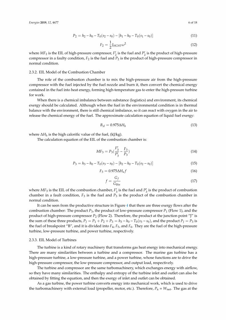
2.3.2. EIL Model of the Combustion Chamber

The role of the combustion chamber is to mix the high-pressure air from the high-pressurecompressor with the fuel injected by the fuel nozzle and burn it, then convert the chemical energycontained in the fuel into heat energy, forming high-temperature gas to enter the high-pressure turbinefor work.

When there is a chemical imbalance between substance (logistics) and environment, its chemicalexergy should be calculated. Although when the fuel in the environmental condition is in thermalbalance with the environment, there is still chemical imbalance, so it can react with oxygen in the air torelease the chemical energy of the fuel. The approximate calculation equation of liquid fuel exergy:

Bxl = 0.975∆Hh (13)

where ∆Hh is the high calorific value of the fuel, (kJ/kg).The calculation equation of the EIL of the combustion chamber is:

MF3 = P3(F′3P′3−

F3

P3) (14)

P3 = h3 − h0 − T0(s3 − s0) − [h2 − h0 − T0(s2 − s0)] (15)

F3 = 0.975∆Hu f (16)

f =G f

GBin(17)

where MF3 is the EIL of the combustion chamber, F′3 is the fuel and P′3 is the product of combustionchamber in a fault condition, F3 is the fuel and P3 is the product of the combustion chamber innormal condition.

It can be seen from the productive structure in Figure 4 that there are three exergy flows after thecombustion chamber: The product P3, the product of low-pressure compressor P1 (Flow 1), and theproduct of high-pressure compressor P2 (Flow 2). Therefore, the product at the junction point “J” isthe sum of these three products, PJ = P1 + P2 + P3 = h3 − h0 − T0(s3 − s0), and the product PJ = P3 isthe fuel of breakpoint “B”, and it is divided into F4, F5, and F6. They are the fuel of the high-pressureturbine, low-pressure turbine, and power turbine, respectively.

2.3.3. EIL Model of Turbines

The turbine is a kind of rotary machinery that transforms gas heat energy into mechanical energy.There are many similarities between a turbine and a compressor. The marine gas turbine has ahigh-pressure turbine, a low-pressure turbine, and a power turbine, whose functions are to drive thehigh-pressure compressor, the low-pressure compressor, and output load, respectively.

The turbine and compressor are the same turbomachinery, which exchanges energy with airflow,so they have many similarities. The enthalpy and entropy of the turbine inlet and outlet can also beobtained by fitting the equation, and then the exergy of inlet and outlet can be obtained.

As a gas turbine, the power turbine converts energy into mechanical work, which is used to drivethe turbomachinery with external load (propeller, motor, etc.). Therefore, P6 = Wnet. The gas at the

Energies 2019, 12, 4677 7 of 18

outlet of the low-pressure turbine is expanded for the last time in the power turbine to output externalmechanical power and exhaust gas. For the exhaust, this paper considers that there is no waste heatboiler and other devices, the exhaust is discharged to the atmospheric environment, and this energy isconsidered to be 0.

In addition, for the P4 and P5 flows in the productive structure diagram, they are the energy thatthe low-pressure turbine and the high-pressure turbine drive the low-pressure compressor and thehigh-pressure compressor to rotate. Both of these energies are mechanical energy. All mechanicalenergy is available energy.

The calculation equation of the EIL of the high-pressure turbine is:

MF4 = P4(F′4P′4−

F4

P4) (18)

P4 =12

JHCHTω2 (19)

F4 = h3 − h0 − T0(s3 − s0) − [h4 − h0 − T0(s4 − s0)] (20)

where MF4 is the EIL of high-pressure turbine, F′4 is the fuel and P′4 is the product of high-pressure turbinein a fault condition, F4 is the fuel and P4 is the product of high-pressure turbine in normal condition.

The calculation equation of the EIL of the low-pressure turbine is:

MF5 = P5(F′5P′5−

F5

P5) (21)

P5 =12

JLCLTω2 (22)

F5 = h4 − h0 − T0(s4 − s0) − [h5 − h0 − T0(s5 − s0)] (23)

where MF5 is the EIL of the low-pressure turbine, F′5 is the fuel and P′5 is the product of low-pressureturbine in a fault condition, F5 is the fuel and P5 is the product of low-pressure turbine innormal condition.

The calculation equation of the EIL of power turbine is:

MF6 = P6(F′6P′6−

F6

P6) (24)

P6 = Wnet (25)

F6 = h6 − h0 − T0(s6 − s0) (26)

where MF6 is the EIL of power turbine, F′6 is the fuel and P′6 is the product of power turbine in a faultycondition, F6 and P6 are the fuel and product of power turbine in normal condition.

The change of unit exergy consumption reflects the change of component exergy efficiency, whichdefines the internal EIL of the equipment. This index is a problem that needs to be explored for thevariation law of the equipment in case of failure and the variation law under the influence of multipleboundary conditions. This problem will be discussed in detail in Section 4.

2.4. Gas Turbine Exergy Loss Analysis Under Normal Conditions

First, the correlation matrix is introduced. The correlation matrix is the matrix connecting eachexergy flow and each component in the system. If the system includes m component and n exergyflow, its correlation matrix is A(m × n), and its element aij is expressed by the following method.When the exergy flow is input into the component i, it is recorded as aij = 1; when the exergy flow isoutput from the component, it is recorded as aij = −1; when neither input nor output, it is recorded

Energies 2019, 12, 4677 8 of 18

as aij = 0. Through the correlation matrix, the characteristics of the whole system can be described.After introducing the correlation matrix, the exergy balance of the system can be written as

A × E = I (27)

where E is the exergy flow vector [0, P1, P2, F3, PJ, B3, F5, F6, F4, F1, F2, P6]; I is the exergy loss [I1, I2,. . . , I12] of each component. Through the correlation matrix A and exergy flow direction E obtainedfrom the above equations, and through exergy balance expression, exergy loss I is obtained, where A isas shown in the equation.

A =

0 −1 0 0 0 0 0 0 0 1 0 00 0 −1 0 0 0 0 0 0 0 1 00 0 0 1 −1 0 0 0 0 0 0 00 0 0 0 0 0 0 0 1 0 −1 00 0 0 0 0 0 1 0 0 −1 0 00 0 0 0 0 0 0 1 0 0 0 −10 1 1 0 1 −1 0 0 0 0 0 00 0 0 0 0 1 −1 −1 −1 0 0 0

Thus, the EIL of each component can be obtained. According to the above equations, a gas turbine

EIL model is established, which will be verified in Section 4.

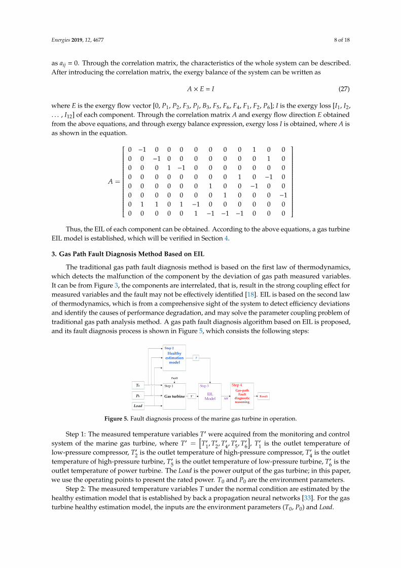
3. Gas Path Fault Diagnosis Method Based on EIL

The traditional gas path fault diagnosis method is based on the first law of thermodynamics,which detects the malfunction of the component by the deviation of gas path measured variables.It can be from Figure 3, the components are interrelated, that is, result in the strong coupling effect formeasured variables and the fault may not be effectively identified [18]. EIL is based on the second lawof thermodynamics, which is from a comprehensive sight of the system to detect efficiency deviationsand identify the causes of performance degradation, and may solve the parameter coupling problem oftraditional gas path analysis method. A gas path fault diagnosis algorithm based on EIL is proposed,and its fault diagnosis process is shown in Figure 5, which consists the following steps:

Energies 2019, 12, x 9 of 19

on EIL is proposed, and its fault diagnosis process is shown in Figure 5, which consists the following steps:

T 'EIL

Model

Gas-pathFault

diagnostic reasoning

MF

T0

P0

Load

Result

Healthy estimation

modelT

Gas turbine

Step 1

Step 2

Step 4

Fault

Step 3

Figure 5. Fault diagnosis process of the marine gas turbine in operation.

Step 1: The measured temperature variables T ′ were acquired from the monitoring and control system of the marine gas turbine, where

1 2 4 5 6, , , ,T T T T T T′ ′ ′ ′ ′ ′= , 1T ′ is the outlet temperature of low-

pressure compressor, 2T ′ is the outlet temperature of high-pressure compressor,

4T ′ is the outlet temperature of high-pressure turbine,

5T ′ is the outlet temperature of low-pressure turbine, 6T ′ is

the outlet temperature of power turbine. The Load is the power output of the gas turbine; in this paper, we use the operating points to present the rated power. T0 and P0 are the environment parameters.

Step 2: The measured temperature variables T under the normal condition are estimated by the healthy estimation model that is established by back a propagation neural networks [33]. For the gas turbine healthy estimation model, the inputs are the environment parameters (T0, P0) and Load.

Step 3: The endogenous irreversible loss MF of the gas turbine components under given conditions are calculated by the EIL model, which is presented in Section 2.

Step 4: The EIL model output describes the characteristics of the gas turbine under normal condition and different faulty conditions, and the diagnostic rule was obtained by statical analysis. Therefore, in this paper, a gas path fault reasoning algorithm is proposed, and its flowchart is shown in Figure 6.

Start

Input MF

Rule 0 C0=1

C0=0

Rule 2 Rule nRule 1

C1=1 C2=1 Cn=1

C1=0 C2=0 Cn=0

Fault diagnosis results C=[C0,C1,…,Cn]

Y

N

...

End

Y YYN N N

Figure 6. The flowchart of the fault reasoning algorithm.

Figure 5. Fault diagnosis process of the marine gas turbine in operation.

Step 1: The measured temperature variables T′ were acquired from the monitoring and controlsystem of the marine gas turbine, where T′ =

[T′1, T′2, T′4, T′5, T′6

], T′1 is the outlet temperature of

low-pressure compressor, T′2 is the outlet temperature of high-pressure compressor, T′4 is the outlettemperature of high-pressure turbine, T′5 is the outlet temperature of low-pressure turbine, T′6 is theoutlet temperature of power turbine. The Load is the power output of the gas turbine; in this paper,we use the operating points to present the rated power. T0 and P0 are the environment parameters.

Step 2: The measured temperature variables T under the normal condition are estimated by thehealthy estimation model that is established by back a propagation neural networks [33]. For the gasturbine healthy estimation model, the inputs are the environment parameters (T0, P0) and Load.

Energies 2019, 12, 4677 9 of 18

Step 3: The endogenous irreversible loss MF of the gas turbine components under given conditionsare calculated by the EIL model, which is presented in Section 2.

Step 4: The EIL model output describes the characteristics of the gas turbine under normal conditionand different faulty conditions, and the diagnostic rule was obtained by statical analysis. Therefore, in thispaper, a gas path fault reasoning algorithm is proposed, and its flowchart is shown in Figure 6.

Energies 2019, 12, x 9 of 19

on EIL is proposed, and its fault diagnosis process is shown in Figure 5, which consists the following steps:

T 'EIL

Model

Gas-pathFault

diagnostic reasoning

MF

T0

P0

Load

Result

Healthy estimation

modelT

Gas turbine

Step 1

Step 2

Step 4

Fault

Step 3

Figure 5. Fault diagnosis process of the marine gas turbine in operation.

Step 1: The measured temperature variables T ′ were acquired from the monitoring and control system of the marine gas turbine, where

1 2 4 5 6, , , ,T T T T T T′ ′ ′ ′ ′ ′= , 1T ′ is the outlet temperature of low-

pressure compressor, 2T ′ is the outlet temperature of high-pressure compressor,

4T ′ is the outlet temperature of high-pressure turbine,

5T ′ is the outlet temperature of low-pressure turbine, 6T ′ is

the outlet temperature of power turbine. The Load is the power output of the gas turbine; in this paper, we use the operating points to present the rated power. T0 and P0 are the environment parameters.

Step 2: The measured temperature variables T under the normal condition are estimated by the healthy estimation model that is established by back a propagation neural networks [33]. For the gas turbine healthy estimation model, the inputs are the environment parameters (T0, P0) and Load.

Step 3: The endogenous irreversible loss MF of the gas turbine components under given conditions are calculated by the EIL model, which is presented in Section 2.

Step 4: The EIL model output describes the characteristics of the gas turbine under normal condition and different faulty conditions, and the diagnostic rule was obtained by statical analysis. Therefore, in this paper, a gas path fault reasoning algorithm is proposed, and its flowchart is shown in Figure 6.

Start

Input MF

Rule 0 C0=1

C0=0

Rule 2 Rule nRule 1

C1=1 C2=1 Cn=1

C1=0 C2=0 Cn=0

Fault diagnosis results C=[C0,C1,…,Cn]

Y

N

...

End

Y YYN N N

Figure 6. The flowchart of the fault reasoning algorithm. Figure 6. The flowchart of the fault reasoning algorithm.

In this process, when the endogenous irreversible loss MF input, Rule 0 is used to detect whetherthe current condition is normal or not. If it is Y, the output C0 = 1, and the current condition is normal.If it is N, it indicates that there is a fault, C0 = 0, and then the following n diagnostic rules will beexecuted in parallel. For example, if the MF complies with Rule 1, then the diagnostic result of Ruel 1is C1 = 1, or else if all other rule output is 0, then the current condition is the first fault.

4. Results and Discussion of Fault Diagnosis

In this section, taking a marine three-shaft gas turbine as an example, the simulation results of theEIL under typical gas path fault are obtained, and then a simulation case was carried out to verify thefault diagnosis method based on EIL.

4.1. Exergy Loss Analysis of Marine Gas Turbine Under Normal Condition

The marine three-shaft gas turbine was divided into eight process groups, including six componentsand two virtual process groups. According to the productive structure of a marine three-shaft gasturbine, the marine gas turbine EIL model was established in MATLAB/Simulink, and the step size ofthe model was 0.2 s. The exergy loss of each process component under different operating conditionswere calculated. In this simulation case, T0 = 20 ◦C P0 = 101.325 kPa, and Load was set to 0.5, 0.6, 0.7, 0.8,and 0.9, respectively, where 0.6 means 60% of rated power. Simulation results of exergy loss of marinethree-shaft gas turbine components are shown in Table 1, and the unit is kilojoules per kilogram (kJ/kg).

Table 1. Simulation results of exergy loss of marine three-shaft gas turbine components.

OperatingCondition LC HC CC HT LT PT J B

0.5 16.59 15.62 247.15 69.59 16.45 169.75 0 00.6 17.21 15.98 257.84 73.51 17.14 182.69 0 00.7 18.17 16.34 267.89 77.26 17.78 196.20 0 00.8 18.86 16.78 277.04 80.72 18.39 209.21 0 00.9 19.61 17.05 285.58 83.95 18.97 221.68 0 0

Energies 2019, 12, 4677 10 of 18

It can be seen from the Table 1 that the exergy losses of components are different under the sameoperating condition, the exergy loss of combustion chamber is the highest, which is because the exergyloss is very large in the combustion process, and the exergy loss of power turbine is also relatively high.Therefore, the simulation results are in accordance with the thermodynamic law. The degree of exergyloss for a component only increases slightly with the increase of operating conditions, which indicatesthat exergy loss can be used to characterize the impact of faults on components more stable, and thisadvantage is helpful for fault isolation. The junction point and breakpoint are virtual components,then the exergy loss of them is 0.

4.2. Fault Reasoning Rules of the Typical Gas Path Fault Conditions

4.2.1. Simulation of Gas Turbine EIL Under Fault Condition

The magnitude of the EIL is mainly related to the fault of the system itself, and many scholarsregard it as an important condition of fault isolation. Therefore, the variation law of the EIL under thecomplex boundary conditions, which is the combination of environment temperature and operatingconditions, was studied and analyzed on the marine gas turbine EIL model, and the EIL reasoning ruleof typical gas path fault is obtained.

A total of 35 boundary conditions were set in Figures 7 and 8, consisting of five operating conditions(0.5–0.9) and seven temperature conditions (0–30 ◦C, 5 ◦C steps). The simulation step of the exergybalance simulation model was set to 0.2 s and simulation time set to 1050 s, that is, 5250 simulationexperiments were performed for a typical fault condition, and 11 typical fault conditions, includingnormal condition and 10 fault conditions, are shown in Table 2.Energies 2019, 12, x 11 of 19

Figure 7. The setting of operating conditions.

Figure 8. The setting of environment temperature.

Table 2. Typical fault models of marine gas turbine.

Case LC HC HT LT PT

ηΔ LC Δ LCG ηΔ HC

Δ HCG ηΔ HT Δ HTG ηΔ LT

Δ LTG ηΔ PT PTGΔ

C0 0 0 0 0 0 0 0 0 0 0 C1 −5 0 0 0 0 0 0 0 0 0 C2 0 −5 0 0 0 0 0 0 0 0 C3 0 0 −5 0 0 0 0 0 0 0 C4 0 0 0 −5 0 0 0 0 0 0 C5 0 0 0 0 −5 0 0 0 0 0 C6 0 0 0 0 0 −5 0 0 0 0 C7 0 0 0 0 0 0 −5 0 0 0 C8 0 0 0 0 0 0 0 −5 0 0 C9 0 0 0 0 0 0 0 0 −5 0 C10 0 0 0 0 0 0 0 0 0 −5

In Table 2, Ci represents a kind of component fault state. Where C0 represents normal condition, C1 represents a 5% decrease in low-pressure compressor efficiency, C2 represents a 5% decrease in low-pressure compressor flow, C3 represents a 5% decrease in high-pressure compressor efficiency, C4 represents a 5% decrease in high-pressure compressor flow, C5 represents a 5% decrease in high-pressure turbine efficiency, and C6 represents 5% decreases in high-pressure turbine flow, C7 represents a 5% decrease in low-pressure turbine efficiency, C8 represents a 5% decrease in low-pressure turbine flow, C9 represents a 5% decrease in power turbine efficiency, and C10 represents a 5% decrease in power turbine flow.

4.2.2. Variation Law of Component EIL Under Typical Fault Condition

It can be seen from Figure 5 that there are six temperature-measured variables in the gas turbine monitoring and control system. Therefore, there are four component EIL that can be monitored in practice, that is the low-pressure compressor, the high-pressure compressor, the low-pressure turbine, and the power turbine. The fault factors were implanted in the EIL model to get the distribution of the EIL of each component. Based on the typical fault simulation result in Section 4.2.1, the variation laws of the four component EIL results are shown in Figure 9.

0 200 400 600 800 1000

0.5

1

Cond

ition

0 200 400 600 800 10000

15

30

T 0

Figure 7. The setting of operating conditions.

Energies 2019, 12, x 11 of 19

Figure 7. The setting of operating conditions.

Figure 8. The setting of environment temperature.

Table 2. Typical fault models of marine gas turbine.

Case LC HC HT LT PT

ηΔ LC Δ LCG ηΔ HC

Δ HCG ηΔ HT Δ HTG ηΔ LT

Δ LTG ηΔ PT PTGΔ

C0 0 0 0 0 0 0 0 0 0 0 C1 −5 0 0 0 0 0 0 0 0 0 C2 0 −5 0 0 0 0 0 0 0 0 C3 0 0 −5 0 0 0 0 0 0 0 C4 0 0 0 −5 0 0 0 0 0 0 C5 0 0 0 0 −5 0 0 0 0 0 C6 0 0 0 0 0 −5 0 0 0 0 C7 0 0 0 0 0 0 −5 0 0 0 C8 0 0 0 0 0 0 0 −5 0 0 C9 0 0 0 0 0 0 0 0 −5 0 C10 0 0 0 0 0 0 0 0 0 −5

In Table 2, Ci represents a kind of component fault state. Where C0 represents normal condition, C1 represents a 5% decrease in low-pressure compressor efficiency, C2 represents a 5% decrease in low-pressure compressor flow, C3 represents a 5% decrease in high-pressure compressor efficiency, C4 represents a 5% decrease in high-pressure compressor flow, C5 represents a 5% decrease in high-pressure turbine efficiency, and C6 represents 5% decreases in high-pressure turbine flow, C7 represents a 5% decrease in low-pressure turbine efficiency, C8 represents a 5% decrease in low-pressure turbine flow, C9 represents a 5% decrease in power turbine efficiency, and C10 represents a 5% decrease in power turbine flow.

4.2.2. Variation Law of Component EIL Under Typical Fault Condition

It can be seen from Figure 5 that there are six temperature-measured variables in the gas turbine monitoring and control system. Therefore, there are four component EIL that can be monitored in practice, that is the low-pressure compressor, the high-pressure compressor, the low-pressure turbine, and the power turbine. The fault factors were implanted in the EIL model to get the distribution of the EIL of each component. Based on the typical fault simulation result in Section 4.2.1, the variation laws of the four component EIL results are shown in Figure 9.

0 200 400 600 800 1000

0.5

1

Cond

ition

0 200 400 600 800 10000

15

30

T 0

Figure 8. The setting of environment temperature.

Table 2. Typical fault models of marine gas turbine.

CaseLC HC HT LT PT

∆ηLC ∆GLC ∆ηHC ∆GHC ∆ηHT ∆GHT ∆ηLT ∆GLT ∆ηPT ∆GPT

C0 0 0 0 0 0 0 0 0 0 0C1 −5 0 0 0 0 0 0 0 0 0C2 0 −5 0 0 0 0 0 0 0 0C3 0 0 −5 0 0 0 0 0 0 0C4 0 0 0 −5 0 0 0 0 0 0C5 0 0 0 0 −5 0 0 0 0 0C6 0 0 0 0 0 −5 0 0 0 0C7 0 0 0 0 0 0 −5 0 0 0C8 0 0 0 0 0 0 0 −5 0 0C9 0 0 0 0 0 0 0 0 −5 0C10 0 0 0 0 0 0 0 0 0 −5

Energies 2019, 12, 4677 11 of 18

In Table 2, Ci represents a kind of component fault state. Where C0 represents normal condition,C1 represents a 5% decrease in low-pressure compressor efficiency, C2 represents a 5% decrease in low-pressurecompressor flow, C3 represents a 5% decrease in high-pressure compressor efficiency, C4 represents a 5%decrease in high-pressure compressor flow, C5 represents a 5% decrease in high-pressure turbine efficiency,and C6 represents 5% decreases in high-pressure turbine flow, C7 represents a 5% decrease in low-pressureturbine efficiency, C8 represents a 5% decrease in low-pressure turbine flow, C9 represents a 5% decrease inpower turbine efficiency, and C10 represents a 5% decrease in power turbine flow.

4.2.2. Variation Law of Component EIL Under Typical Fault Condition

It can be seen from Figure 5 that there are six temperature-measured variables in the gas turbinemonitoring and control system. Therefore, there are four component EIL that can be monitored inpractice, that is the low-pressure compressor, the high-pressure compressor, the low-pressure turbine,and the power turbine. The fault factors were implanted in the EIL model to get the distribution of theEIL of each component. Based on the typical fault simulation result in Section 4.2.1, the variation lawsof the four component EIL results are shown in Figure 9.Energies 2019, 12, x 12 of 19

C1 C2 C3 C4 C5 C6 C7 C8 C9 C10-2

0

2

4

6

8

LC

MFminMFRange

C1 C2 C3 C4 C5 C6 C7 C8 C9 C10 2−

024

6

8

LC

MF_minMF_Range

(a) EIL range of low-pressure compressor.

C1 C2 C3 C4 C5 C6 C7 C8 C9 C10-2

0

2

4

6

HC

MFminMFRange

C1 C2 C3 C4 C5 C6 C7 C8 C9 C10 2−

0

2

4

6

HC

MF_minMF_Range

(b) EIL range of high-pressure compressor

C1 C2 C3 C4 C5 C6 C7 C8 C9 C10-2

0

2

4

6

LT

MFminMFRange

C1 C2 C3 C4 C5 C6 C7 C8 C9 C10 2−

0

2

4

6

LT

MF_minMF_Range

(c) EIL range of low-pressure turbine

C1 C2 C3 C4 C5 C6 C7 C8 C9 C10-10

0

10

20

30

PT

MFminMFRange

C1 C2 C3 C4 C5 C6 C7 C8 C9 C10 10−

10

0

20

30

PT

MF_minMF_Range

(d) EIL range of power turbine

Figure 9. Distribution law of the EIL of various systems under marine gas turbine failure.

The maximum value, minimum value, and standard deviation of each component EIL under typical fault condition were obtained. Take C1 (5% decrease in low-pressure compressor efficiency) as an example, the maximum value, minimum value, and standard deviation of the EIL under 35 boundary conditions are shown in Table 3.

Figure 9. Distribution law of the EIL of various systems under marine gas turbine failure.

Energies 2019, 12, 4677 12 of 18

The maximum value, minimum value, and standard deviation of each component EIL undertypical fault condition were obtained. Take C1 (5% decrease in low-pressure compressor efficiency)as an example, the maximum value, minimum value, and standard deviation of the EIL under 35boundary conditions are shown in Table 3.

Table 3. The variation law of the EIL under typical fault condition C1.

Parameter LC HC LT PT

MF_max 6.48 0.01 0.11 13.16MF_min 5.38 −0.38 −0.04 9.50MF_std 0.27 0.02 0.01 0.50

From Figure 9, it can clearly be seen that the distribution range of the EIL of each component isunique when different faults occurred. Therefore, it is feasible to use the EIL for fault detection andisolation of the marine three-shaft gas turbine.

4.2.3. Gas Path Fault Reasoning Rules

Firstly, the false alarm rate Fr and missing alarm rate Mr are introduced as fault diagnosis criteria.

Fr =M

R− T× 100% (28)

Mr =NT× 100% (29)

where M is the number of the false alarm, N is the number of missing alarm, T is the number ofexperiment samples for each fault pattern, and R is the total number of experiment samples.

It is necessary to judge whether there is a fault in the system. When there is no fault, the EIL ofthe marine gas turbine component should be zero in theory. However, in practice, due to the noise,the EIL of the system is not zero, but a very small number close to zero. Therefore, for the reasoningrule of the normal condition, the setting of the threshold value of the EIL needs to be discussed.

∩ abs(MFi) < X (30)

where i represents the components of the marine gas turbine, and X represents the value of thethreshold. Suppose X equals 0.1, 0.2, 0.3, 0.4, and 0.5 respectively, and the false alarm rate and missingalarm rate are shown in Table 4, respectively.

Table 4. Relationship between the threshold and diagnostic criteria.

X Fr Mr

0.1 6.52% 0.04%0.2 5.84% 0%0.3 5.48% 0%0.4 5.12% 0.04%0.5 4.880% 0.08%

It can be seen from the table that the false alarm rate Fr has a slight downward trend withincreasing the threshold, while the missing alarm rate Mr is zero when X equals 0.2 or 0.3.

On the basis of the gas path fault diagnosis method introduced in Section 3, according to the EILdistribution of components under 10 typical fault conditions in Figure 9, the fault reasoning rules areshown in Table 5.

Energies 2019, 12, 4677 13 of 18

Table 5. Fault reasoning rules of the marine three-shaft gas turbine.

Number Condition Fault Vector

Rule 0 0 ≤∣∣∣MF(i)

∣∣∣ < 0.3 [1 0 0 0 0 0 0 0 0 0 0]Rule 1 5.38 ≤MFLC ≤ 6.48 [0 1 0 0 0 0 0 0 0 0 0]

Rule 20.001 < MFLC ≤ 0.77 & 0.001 < MFPT ≤ 1.55

&− 0.07 ≤MFHC ≤ 0.01[0 0 1 0 0 0 0 0 0 0 0]

Rule 3 4.40 ≤MFHC ≤ 5.29 [0 0 0 1 0 0 0 0 0 0 0]

Rule 4 MFLC ≤ −0.001 & 0.64 ≤MFHC ≤ 1.11& − 0.04 ≤MFLT ≤ 0.01 & 0.63 ≤MFPT ≤ 1.70 [0 0 0 0 1 0 0 0 0 0 0]

Rule 5 9.67 ≤MFPT ≤ 13.16 [0 0 0 0 0 1 0 0 0 0 0]

Rule 6MFLC > 0.001 & MFHC < −0.001

& −3.92 ≤MFLT ≤ −2.67 & −4.23 ≤MFPT ≤ −1.96 [0 0 0 0 0 0 1 0 0 0 0]

Rule 7 3.67 ≤MFLT ≤ 4.36 [0 0 0 0 0 0 0 1 0 0 0]

Rule 8MFLC < −0.001 & MFHC < −0.001

& −1.43 ≤MFLT ≤ −1.08 & −6.05 ≤MFPT ≤ −2.50 [0 0 0 0 0 0 0 0 1 0 0]

Rule 9 16.30 ≤MFPT ≤ 26.21 [0 0 0 0 0 0 0 0 0 1 0]

Rule 100.43 < MFLC < 1.50 & −0.05 < MFHC ≤ 0.22

& 1.51 < MFLT ≤ 2.01 & 1.77 < MFPT ≤ 3.77 [0 0 0 0 0 0 0 0 0 0 1]

According to Figure 6, IF and ELSE-IF logic statements are used to fault reasoning, and the faultdiagnosis result is expressed in the fault vector C.

4.3. Fault Diagnosis of Marine Gas Turbine

In this section, using the marine gas turbine model to present the actual marine gas turbine [33],which was established in Matlab/Simulink, and the simulation method is the fourth-order ode14x(extrapolation with fixed time step), the simulation step is 0.2 s. In the test case, the gas turbine worksunder the transient condition, the operating condition is increased from 0.5 to 0.9 in 500 s with thevariable environment temperature that is between 0 and 30 ◦C, as shown in Figures 10 and 11.

Energies 2019, 12, x 14 of 19

Table 5. Fault reasoning rules of the marine three-shaft gas turbine.

Number Condition Fault Vector

Rule 0 ( )0 0.3MF i≤ < [1 0 0 0 0 0 0 0 0 0 0]

Rule 1 ≤ ≤5.38 6.48LCM F [0 1 0 0 0 0 0 0 0 0 0]

Rule 2 0.001 0.77 & 0.001 1.55& 0.07 0.01

LC PT

HC

MF MFMF

< ≤ < ≤− ≤ ≤

[0 0 1 0 0 0 0 0 0 0 0]

Rule 3 ≤ ≤4.40 5.29H CM F [0 0 0 1 0 0 0 0 0 0 0]

Rule 4 0.001 & 0.64 1.11

& 0.04 0.01 & 0.63 1.70LC HC

LT PT

MF MFMF MF

≤ − ≤ ≤− ≤ ≤ ≤ ≤

[0 0 0 0 1 0 0 0 0 0 0]

Rule 5 ≤ ≤9.67 13.16PTM F [0 0 0 0 0 1 0 0 0 0 0]

Rule 6 0.001 & 0.001

& 3.92 2.67 & 4.23 1.96LC HC

LT PT

MF MFMF MF

> < −− ≤ ≤ − − ≤ ≤ −

[0 0 0 0 0 0 1 0 0 0 0]

Rule 7 ≤ ≤3.67 4.36LTM F [0 0 0 0 0 0 0 1 0 0 0]

Rule 8 0.001 & 0.001

& -1.43 -1.08 & -6.05 -2.50LC HC

LT PT

MF MFMF MF

< − < −≤ ≤ ≤ ≤

[0 0 0 0 0 0 0 0 1 0 0]

Rule 9 ≤ ≤16.30 26.21PTM F [0 0 0 0 0 0 0 0 0 1 0]

Rule 10 0.43 1.50 & 0.05 0.22& 1.51 2.01 & 1.77 3.77

LC HC

LT PT

MF MFMF MF

< < − < ≤< ≤ < ≤

[0 0 0 0 0 0 0 0 0 0 1]

4.3. Fault Diagnosis of Marine Gas Turbine

In this section, using the marine gas turbine model to present the actual marine gas turbine [33], which was established in Matlab/Simulink, and the simulation method is the fourth-order ode14x (extrapolation with fixed time step), the simulation step is 0.2 s. In the test case, the gas turbine works under the transient condition, the operating condition is increased from 0.5 to 0.9 in 500 s with the variable environment temperature that is between 0 and 30 °C, as shown in Figures 10 and 11.

Suppose gas turbine works in 30 s under normal condition 0C , then a fault occurred for 20 s.

Ten typical faulty conditions 1 2 10, , ,C C C occurred separately in sequence. The fault simulation setting is shown in Figure 12. Therefore, the total number of test samples is 2501, the number of normal test samples is 1001, and the number of test samples for each fault is 150.

The measured variables under the normal condition are on-line estimate by the healthy estimation model, then using the EIL model to calculate the EIL of each component under this test case, and the results of the EIL are shown in Figure 13.

Figure 13. shows the change process of the EILs of the low-pressure compressor, high-pressure compressor, low-pressure turbine, and power turbine, and the EIL will change abruptly at the moment of gas path fault implantation.

Figure 10. The operating condition setting of marine gas turbine.

0 100 200 300 400 5000.4

0.5

0.6

0.7

0.8

0.9

1

Time(s)

Con

ditio

n

Commented [M1]: Please confirm if this is correct.

Please confirm what the “x” represents.

we have modofied ‘ode14 x’ to ‘ode14x’,which is a fixed step

continous solver to solve a stiff system in Matlab/Simulink.

Figure 10. The operating condition setting of marine gas turbine.Energies 2019, 12, x 15 of 19

Figure 11. The ambient temperature setting of marine gas turbine.

Figure 12. Settings of simulation fault.

100 200 300 400 500

100 200 300 400 500

100 200 300 400 500

100 200 300 400 500

50−

0

5020−

20

0

0

0

10−

10

10

10−

Time(s)

Figure 13. Component EIL change of marine gas turbine under simulated fault.

Finally, the MFs of component EIL input the fault reasoning algorithm. Rule 0 is used to detect the current status of the marine gas turbine, whether it is normal or not. The diagnosis result is μ 0

, 1 represents the normal condition, and 0 represents the faulty condition. When a fault is detected, ten typical fault reasoning rules execute in parallel to isolate which fault occurred, the fault reasoning results are μ μ1 10~ , which is the value of element

1 10, ,C C of fault vector C. The fault reasoning results are shown in Figure 14, and it shows that the marine gas turbine diagnosis method based on

0 100 200 300 400 500

0

10

20

30

Time(s)

T 0(℃)

Figure 11. The ambient temperature setting of marine gas turbine.

Suppose gas turbine works in 30 s under normal condition C0, then a fault occurred for 20 s.Ten typical faulty conditions C1, C2, · · · , C10 occurred separately in sequence. The fault simulationsetting is shown in Figure 12. Therefore, the total number of test samples is 2501, the number of normaltest samples is 1001, and the number of test samples for each fault is 150.

Energies 2019, 12, 4677 14 of 18

Energies 2019, 12, x 15 of 19

Figure 11. The ambient temperature setting of marine gas turbine.

Figure 12. Settings of simulation fault.

100 200 300 400 500

100 200 300 400 500

100 200 300 400 500

100 200 300 400 500

50−

0

5020−

20

0

0

0

10−

10

10

10−

Time(s)

Figure 13. Component EIL change of marine gas turbine under simulated fault.

Finally, the MFs of component EIL input the fault reasoning algorithm. Rule 0 is used to detect the current status of the marine gas turbine, whether it is normal or not. The diagnosis result is μ 0

, 1 represents the normal condition, and 0 represents the faulty condition. When a fault is detected, ten typical fault reasoning rules execute in parallel to isolate which fault occurred, the fault reasoning results are μ μ1 10~ , which is the value of element

1 10, ,C C of fault vector C. The fault reasoning results are shown in Figure 14, and it shows that the marine gas turbine diagnosis method based on

0 100 200 300 400 500

0

10

20

30

Time(s)

T 0(℃)

Figure 12. Settings of simulation fault.

The measured variables under the normal condition are on-line estimate by the healthy estimationmodel, then using the EIL model to calculate the EIL of each component under this test case, and theresults of the EIL are shown in Figure 13.

Energies 2019, 12, x 15 of 19

Figure 11. The ambient temperature setting of marine gas turbine.

Figure 12. Settings of simulation fault.

100 200 300 400 500

100 200 300 400 500

100 200 300 400 500

100 200 300 400 500

50

0

50

20

20

0

0

0

10

10

10

10

LC

MF

HC

MF

LT

MF

PT

MF

Time(s)

Figure 13. Component EIL change of marine gas turbine under simulated fault.

Finally, the MFs of component EIL input the fault reasoning algorithm. Rule 0 is used to detect

the current status of the marine gas turbine, whether it is normal or not. The diagnosis result is 0

,

1 represents the normal condition, and 0 represents the faulty condition. When a fault is detected, ten

typical fault reasoning rules execute in parallel to isolate which fault occurred, the fault reasoning

results are 1 10

~ , which is the value of element 1 10, ,C C of fault vector C. The fault reasoning

results are shown in Figure 14, and it shows that the marine gas turbine diagnosis method based on

0 100 200 300 400 500

0

10

20

30

Time(s)

T0(℃

)

Figure 13. Component EIL change of marine gas turbine under simulated fault.

Figure 13 shows the change process of the EILs of the low-pressure compressor, high-pressurecompressor, low-pressure turbine, and power turbine, and the EIL will change abruptly at the momentof gas path fault implantation.

Finally, the MFs of component EIL input the fault reasoning algorithm. Rule 0 is used to detectthe current status of the marine gas turbine, whether it is normal or not. The diagnosis result is µ0,1 represents the normal condition, and 0 represents the faulty condition. When a fault is detected,ten typical fault reasoning rules execute in parallel to isolate which fault occurred, the fault reasoningresults are µ1 ∼ µ10, which is the value of element C1, · · · , C10 of fault vector C. The fault reasoningresults are shown in Figure 14, and it shows that the marine gas turbine diagnosis method based onEIL can diagnose the gas path fault correctly. The EIL has good sensitivity to the gas path fault, thereasoning rule will change in time when the hypothesis fault occurred. At the same time, throughexperiments, it is found that missing alarms generally occur at the switching time of normal conditionand fault condition, so the fault detection time is introduced, which is the product of the time step andthe missing alarm. The false alarm, missing alarm, and detection time are shown in Table 6.

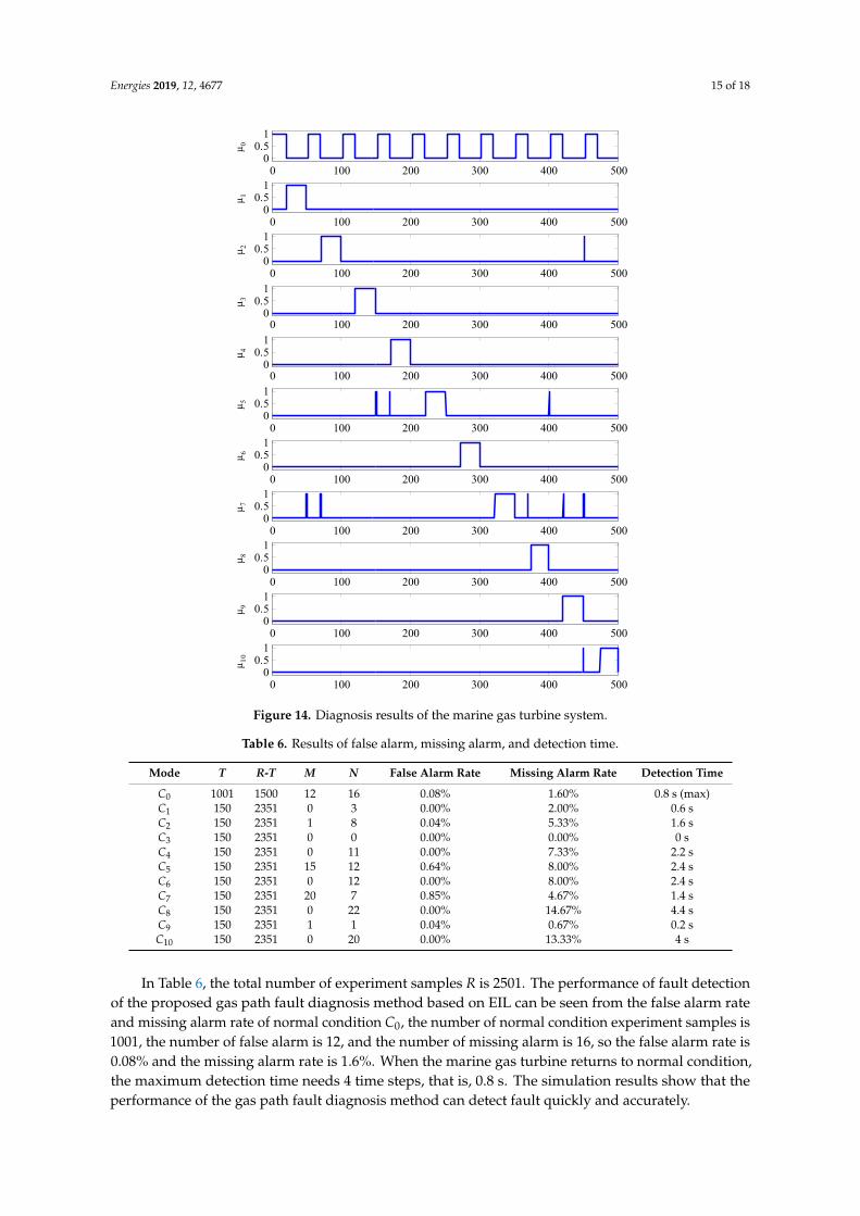
Energies 2019, 12, 4677 15 of 18

Energies 2019, 12, x 16 of 19

EIL can diagnose the gas path fault correctly. The EIL has good sensitivity to the gas path fault, the reasoning rule will change in time when the hypothesis fault occurred. At the same time, through experiments, it is found that missing alarms generally occur at the switching time of normal condition and fault condition, so the fault detection time is introduced, which is the product of the time step and the missing alarm. The false alarm, missing alarm, and detection time are shown in Table 6.

Figure 14. Diagnosis results of the marine gas turbine system.

In Table 6, the total number of experiment samples R is 2501. The performance of fault detection of the proposed gas path fault diagnosis method based on EIL can be seen from the false alarm rate and missing alarm rate of normal condition C0, the number of normal condition experiment samples is 1001, the number of false alarm is 12, and the number of missing alarm is 16, so the false alarm rate is 0.08% and the missing alarm rate is 1.6%. When the marine gas turbine returns to normal condition,

0 100 200 300 400 5000

0.51

μ 0

0 100 200 300 400 5000

0.51

μ 1

0 100 200 300 400 5000

0.51

μ 2

0 100 200 300 400 5000

0.51

μ 3

0 100 200 300 400 5000

0.51

μ 4

0 100 200 300 400 5000

0.51

μ 5

0 100 200 300 400 5000

0.51

μ 6

0 100 200 300 400 5000

0.51

μ 7

0 100 200 300 400 5000

0.51

μ 8

0 100 200 300 400 5000

0.51

μ 9

0 100 200 300 400 5000

0.51

μ 10

Figure 14. Diagnosis results of the marine gas turbine system.

Table 6. Results of false alarm, missing alarm, and detection time.

Mode T R-T M N False Alarm Rate Missing Alarm Rate Detection Time

C0 1001 1500 12 16 0.08% 1.60% 0.8 s (max)C1 150 2351 0 3 0.00% 2.00% 0.6 sC2 150 2351 1 8 0.04% 5.33% 1.6 sC3 150 2351 0 0 0.00% 0.00% 0 sC4 150 2351 0 11 0.00% 7.33% 2.2 sC5 150 2351 15 12 0.64% 8.00% 2.4 sC6 150 2351 0 12 0.00% 8.00% 2.4 sC7 150 2351 20 7 0.85% 4.67% 1.4 sC8 150 2351 0 22 0.00% 14.67% 4.4 sC9 150 2351 1 1 0.04% 0.67% 0.2 sC10 150 2351 0 20 0.00% 13.33% 4 s

In Table 6, the total number of experiment samples R is 2501. The performance of fault detectionof the proposed gas path fault diagnosis method based on EIL can be seen from the false alarm rateand missing alarm rate of normal condition C0, the number of normal condition experiment samples is1001, the number of false alarm is 12, and the number of missing alarm is 16, so the false alarm rate is0.08% and the missing alarm rate is 1.6%. When the marine gas turbine returns to normal condition,the maximum detection time needs 4 time steps, that is, 0.8 s. The simulation results show that theperformance of the gas path fault diagnosis method can detect fault quickly and accurately.

Energies 2019, 12, 4677 16 of 18

The performance of fault isolation of the proposed gas path fault diagnosis based on EIL can beseen from the false alarm rate and missing alarm rate of the fault condition C1, C2, . . . , C10. Althoughthe missing alarm rate is slightly higher, the proposed gas path fault diagnosis method can isolate faultaccurately. The false alarm rate is less than 1% which shows that the diagnostic reasoning rules basedon EIL are robust under complex operating conditions and environments.

The missing alarm of C8 and C10 is high, because the transition time from the normal condition tofault condition of the marine gas turbine model is long in the simulation test.

5. Conclusions

In this paper, a gas path fault diagnosis method based on EIL has been presented to detect andisolate the gas path faults of marine gas turbines. The EIL of component models were established tocharacterize exergy loss under the normal condition and typical gas path fault condition. The EIL issensitive to gas path fault, and it is not affected by the change of operating condition and environment.Therefore, the diagnostic reasoning rules based on EIL are robust, and are helpful for detecting andisolating gas path faulty components.

Simulation case studies on a three-shaft marine gas turbine were conducted, and the performanceof the proposed method for the detection and isolation of typical gas path fault was analyzed.The simulation results show that the proposed EIL-based gas path fault diagnosis method detect andisolate gas path fault accurately.

In this paper, the feasibility of the gas path fault diagnosis based on EIL was verified by single gaspath fault. In the future, we will improve the performance of the proposed method under transientprocess. Furthermore, we will continually evaluate the multiple gas path fault diagnosis performanceof the proposed method and also study hybrid diagnostic approaches combining EIL with artificialintelligence algorithms.

Author Contributions: This research was completed through a collaboration of all authors. Y.C. and J.L. proposedthe fault diagnosis based on EIL and wrote the original manuscript; S.L. was the team leader of this work andresponsible for coordination; G.H., X.L., and Y.C. designed the case studies and analyzed the results.

Funding: This research was funded by the National Science and Technology Major Project (2017-I-0007-0008) andthe Fundamental Research Funds for the Central Universities (HEUCFP201722).

Conflicts of Interest: The authors declare no conflicts of interest.

References

1. Volponi, A.J. Gas Turbine Engine Health Management: Past, Present, and Future Trends. J. Eng. Gas TurbinesPower 2014, 136, 051201. [CrossRef]

2. Tahan, M.; Tsoutsanis, E.; Muhammad, M. Performance-based health monitoring, diagnostics and prognosticsfor condition-based maintenance of gas turbines: A review. Appl. Energy 2017, 198, 122–144. [CrossRef]

3. Li, Y.G. Gas turbine performance and health status estimation using adaptive gas path analysis. J. Eng. Gas.Turbines Power 2010, 132, 041701. [CrossRef]

4. Ying, Y.; Cao, Y.P.; Li, S. Study on gas turbine engine fault diagnostic approach with a hybrid of gray relationtheory and gas-path analysis. Adv. Mech. Eng. 2016, 8, 1687814015627769. [CrossRef]

5. Simon, D.L.; Bird, J.; Davison, C.; Volponi, A.; Iverson, R.E. Bench marking gas path diagnostic methods:A public approach. In Proceedings of the ASME Turbo Expo 2008: Power for Land, Sea, and Air, Berlin,Germany, 9–13 June 2008; pp. 325–336.

6. Kyriazis, A.; Mathioudakis, K. Gas Turbine Fault Diagnosis Using Fuzzy-Based Decision Fusion. J. Propuls.Power 2009, 25, 335–343. [CrossRef]

7. Amare, F.D.; Gilani, S.I.; Aklilu, B.T. Two-shaft stationary gas turbine engine gas path diagnostics usingfuzzy logic. J. Mech. Sci. Technol. 2017, 31, 5593–5602. [CrossRef]

8. Zaidan, M.A.; Mills, A.R.; Harrison, R.F.; Fleming, P.J. Gas turbine engine prognostics using Bayesianhierarchical models: A variational approach. Mech. Syst. Sig. Proc. 2016, 70, 120–140. [CrossRef]

Energies 2019, 12, 4677 17 of 18

9. Zaidan, M.A.; Mills, A.R.; Harrison, R.F.; Fleming, P.J. Bayesian hierarchical models for aerospace gas turbineengine prognostics. Expert Syst. Appl. 2015, 42, 539–553. [CrossRef]

10. Romessis, C.; Stamatis, A.; Mathioudakis, K. Setting up a belief network for turbofan diagnosis with the aidof an engine performance model. ISABE Pap. 2001, 1032, 19–26.

11. Cao, Y.P.; Li, S.Y.; Yi, S.; Zhao, N.B. Fault diagnosis of a gas turbine gas fuel system using a self-organizingnetwork. Adv. Sci. Lett. 2012, 8, 386–392. [CrossRef]

12. Talaat, M.; Gobran, M.H.; Wasfi, M. A hybrid model of an artificial neural network with thermodynamic modelfor system diagnosis of electrical power plant gas turbine. J. Eng. Appl. Artif. Intell. 2018, 68, 222–235. [CrossRef]

13. Zedda, M.; Singh, R. Gas Turbine Engine and Sensor Fault Diagnosis Using Optimization Techniques.J. Propuls. Power 2002, 18, 1019–1025. [CrossRef]

14. Alfredo, G.; Raniero, S. A multi-variable multi-objective methodology for experimental data and thermodynamicanalysis validation: An application to micro gas turbines. J. Appl. Therm. Eng. 2018, 134, 501–512. [CrossRef]

15. Meskin, N.; Naderi, E.; Khorasani, K. A Multiple Model-Based Approach for Fault Diagnosis of Jet Engines.IEEE Trans. Control Syst. Technol. 2013, 21, 254–262. [CrossRef]

16. Yang, Q.; Li, S.; Cao, Y. A Gas Path Fault Contribution Matrix for Marine Gas Turbine Diagnosis Based on aMultiple Model Fault Detection and Isolation Approach. Energies 2018, 11, 3316. [CrossRef]

17. Keshavarzian, S.; Rocco, M.V.; Colombo, E. Thermoeconomic diagnosis and malfunction decomposition:Methodology improvement of the Thermoeconomic Input-Output Analysis (TIOA). Energy Convers. Manag.2018, 157, 644–655. [CrossRef]

18. Iacentino, A.; Catrini, P. Assessing the Robustness of Thermoeconomic Diagnosis of Fouled Evaporators:Sensitivity Analysis of the Exergetic Performance of Direct Expansion Coils. Entropy 2016, 18, 85. [CrossRef]

19. Direk, M.; Mert, M.S. Comparative and Exergetic Study of a Gas Turbine System with Inlet Air Cooling.Teh. Vjesn. Tech. Gaz. 2018, 25, 306–311. [CrossRef]

20. Fallah, M.; Siyahi, H.; Ghiasi, R.A.; Mahmoudi, S.M.S.; Yari, M.; Rosen, M.A. Comparison of different gasturbine cycles and advanced exergy analysis of the most effective. Energy 2016, 116, 701–715. [CrossRef]

21. Haseli, Y.; Dincer, I.; Naterer, G.F. Exergy analysis of a combined fuel cell and Gas Turbine Power Plant withintercooling and reheating. Int. J. Exergy 2010, 7, 211–231. [CrossRef]

22. Ibrahim, T.K.; Basrawi, F.; Awad, O.I.; Abdullah, A.N.; Najafi, G.; Mamat, R.; Hagos, F.Y. Thermal performanceof gas turbine power plant based on exergy analysis. Appl. Therm. Eng. 2017, 115, 977–985. [CrossRef]

23. Khaliq, A.; Choudhary, K. Exergy analysis of the regenerative gas turbine cycle using absorption inlet coolingand evaporative aftercooling. J. Energy Inst. 2009, 82, 159–167. [CrossRef]

24. Peng, S.; Hong, H. Exergy analysis of solar gas turbine system coupled with Kalina cycle. Int. J. Exergy 2015,18, 192–213. [CrossRef]

25. Sohret, Y.; Ekici, S.; Altuntas, O.; Hepbasli, A.; Karakoc, T.H. Exergy as a useful tool for the performanceassessment of aircraft gas turbine engines: A key review. Prog. Aerosp. Sci. 2016, 83, 57–69. [CrossRef]

26. Cross, A.J.; Longden, A.; Owen, F. A Critical Review of the Thermoeconomic Diagnosis Methodologies for theLocation of Causes of Malfunctions in Energy Systems. J. Energy Resour. Technol. 2003, 128, 345–354. [CrossRef]

27. Verda, V.; Baccino, G. Thermoeconomic Diagnosis Applied to the Transient Operation of a Microturbine.In Proceedings of the ASME 2012 International Mechanical Engineering Congress and Exposition, Houston,TX, USA, 9–15 November 2012; pp. 1579–1588.

28. Oh, H.S.; Lee, Y.; Kwak, H.Y. Diagnosis of Combined Cycle Power Plant Based on ThermoeconomicAnalysis:A Computer Simulation Study. Entrop 2017, 19, 643. [CrossRef]

29. Massardo, A.F.; Scialo, M. Thermoeconomic Analysis of Gas Turbine Based Cycles. J. Eng. Gas Turbines Power1999, 122, 664–671. [CrossRef]

30. Yan, Q.Y.; Yan, Q.S. Analysis of influence factors on irreversible loss and optimization in heat exchanger.In Proceedings of the 3rd International Symposium on Heat Transfer Enhancement and Energy Conservation,Guangzhou, China, 12–15 January 2004; Volume 1–2.

31. Chen, L.E.; Zhu, X.Q.; Sun, F.; Wu, C. Exergy-based ecological optimization for a generalized irreversibleCarnot heat-pump. Appl. Energy 2007, 84, 78–88. [CrossRef]

32. Cheng, X.T.; Liang, X.G. Entransy analyses of heat-work conversion systems with inner irreversiblethermodynamic cycles. Chin. Phys. B 2015, 24. [CrossRef]

Energies 2019, 12, 4677 18 of 18

33. Cao, Y.; He, Y.; Yu, F.; Du, J.; Li, S.; Yang, Q.; Liu, R. A Two-Layer Multi-Model Gas Path Fault Diagnosis Method.In Proceedings of the ASME Turbo Expo 2018: Turbomachinery Technical Conference and Exposition. Volume 6: Ceramics;Controls, Diagnostics, and Instrumentation; Education; Manufacturing Materials and Metallurgy, Oslo, Norway, 11–15June 2018; American Society of Mechanical Engineers Digital Collection: New York, NY, USA, 2018.

34. Torres, C.; Valero, A.; Serra, L.; Royo, J. Structural theory and thermoeconomic diagnosis Part 1. On malfunctionand dysfunction analysis. Energy Convers. Manag. 2002, 43, 1503–1518. [CrossRef]

35. Verda, V.; Serra, L.; Valero, A. Thermoeconomic diagnosis: Zooming strategy applied to highly complexenergy systems. Part 2: On the choice of the productive structure. J. Energy Resour. Technol. Trans. 2005, 127,50–58. [CrossRef]

© 2019 by the authors. Licensee MDPI, Basel, Switzerland. This article is an open accessarticle distributed under the terms and conditions of the Creative Commons Attribution(CC BY) license (http://creativecommons.org/licenses/by/4.0/).