a master 1999
TRANSCRIPT
Timothy Dickinson
A thesis submitted in conformity with the requirements for the degree of Master of Applied Science
Graduate Department of Mechanical Engineering University of Toronto
Copyright @ 1999 by Timothy Dickinson

National Library Bibliotheque nationale du Canada
Acquisitions and Acquisitions et Bibliographie Services services bibliographiques
395 Wellington Street 395. rue WeNingtori OitawaON KIAON4 OctawaON K 1 A W canada Csnada
Our fi& Uînro fdHrr>rr
The author has granted a non- exclusive licence allowing the National Library of Canada to reproduce, loan, distribute or sell copies of this thesis in microform, paper or electronic formats.
L'auteur a accordé une licence non exclusive permettant à la Bibliothèque nationale du Canada de reproduire, prêter, distribuer ou vendre des copies de cette thèse sous la fonne de microfiche/nlm, de reproduction sur papier ou sur format électronique.
The author retains ownership of the L'auteur conserve la propriété du copyright in this thesis. Neither the droit d'auteur qui protège cette thèse. thesis nor substantial extracts fiom it Ni la thèse ni des extraits substantiels may be printed or otheMise de celle-ci ne doivent être imprimés reproduced without the author's ou autrement reproduits sans son permission. autorisation.

Abstract
Good heat exchanger design requires that the designer understands and accounts for fiow-
induced vibration mechanisrns. These mechanisms include vortex shedding, turbulent
excitation and fluideiastic instability. Including the effects of t hese mechanisms in a
vibration analysis of a heat exchanger requires information about damping. Multispan
heat exchanger tube damping consists of three main components: viscous damping dong
the tube, friction and squeeze-film damping at the supports. Unlike viscous damping,
squeeze-film damping is poorly understood and difficult to rneasure. In addition: the
effect of temperature-dependent fluid viscosity on tube damping is not yet understood.
E-xperiments were done with two instrumented test rigs. Each rig contained a single
vertical heat exchanger tube with multiple spms and a random excitation mechanism.
Tests were conducted in air and in water at three different temperatures (25, 60 and
90°C). -4 new computer tool was developed to measure tube response to random exci-
tation. This tool was also used to measure darnping. -4nother new computer tool was
developed to measure energy dissipation rates at the rig supports and the rate of energy
used to excite the tube. The dissipation rate of input energy was also used to calculate
darnping. Results indicate that damping does not change over the range of temperatures
tested. Results also show that measuring energy dissipation rate may be a useful way of
estimating darnping.

Dedicat ion
This thesis is dedicated to my parents, David and Karen Dickinson, who inspired me to
undertake higher levels of leaming; and to my friends Dino Cule and Mark Biegler, wbo
inspired me to complete those levels.

Acknowledgement s
I acknowledge the invaluable efforts of Michel Pet tigrew and Colet t e Taylor, of Atomic
Energy of Canada Limited, and thank them wholeheartedly. Without thern, this work
could not have been initiated or accomplished.
1 acknowledge the guidance of Professor Iain Cume, of the graduate department of
Mechanical Engineering at the University of Toronto, and thank him for his supervision.
His instruction, help, suggestions, experience: and patience were beyond the cal1 of duty.
I acknowledge the assistance of K e q Boucher and Murray Weckwerth, both formerly
of Atomic Energy of Canada Limited, and thank them as well. Both helped me in concept
and practice dong the way.
1 also acknowledge the resources-human , financial, and material-made available
to me by Atornic Energy of Canada Limited and the Natural Sciences and Engineering
Research Council and administered by Michel Pettigrew and Iain Cume. Without those
resources, this work could not have been carried out.
Contents
Abstract
Dedication
Acknowledgements
List of Symbols and Acronyms
List of Tables
List of Figures
ii
iii
iv
ix
xi
xiii
1 Introduction 1
1.1 Problem . . . . . . . . . . . . . . . . . . . . . . . . . . . . . . . . . . . . 2
1 Measuring Damping . . . . . . . . . . . . . . . . . . . . . . . . . 2
1.1.2 The Effect of Temperature on Damping . . . . . . . . . . . . . . . 2
1.2 Approach . . . . . . . . . . . . . . . . . . . . . . . . . . . . . . . . . . . 3
2 Literature Review and Theory 4
2.1 Tube-Support Configurations . . . . . . . . . . . . . . . . . . . . . . . . 4
2.2 Damping . . . . . . . . . . . . . . . . . . . . . . . . . . . . . . . . . . . . 6
2.2.1 Energy Dissipation Mechanisms . . . . . . . . . . . . . . . . . . . 6
2.2.2 Current Design Recommendations . . . . . . . . . . . . . . . . . . 9

2.3 Damping Ratio Caiculation Methods . . . . . . . . . . . . . . . . . . . . 10
2.3.1 CurveFitting . . . . . . . . . . . . . . . . . . . . . . . . . . . . . 11
2.3.2 The Marquardt Method . . . . . . . . . . . . . . . . . . . . . . . 11
2.3.3 Application to Two-Peak Damping Ratios . . . . . . . . . . . . . 13
2.3.4 DifficultieswiththeseMethods . . . . . . . . . . . . . . . . . . . 14
2.4 Work-Rates . . . . . . . . . . . . . . . . . . . . . . . . . . . . . . . . . . 14
2.4.1 Work-Rates as Darnping Ratio Estimators . . . . . . . . . . . . . 15
3 Experimental Procedure 18
3.1 Room-Temperature Multispan Damping K g (RTMDR) . . . . . . . . . . 18
. . . . . . . . . . . . . . . . . . 3.1.1 Construction and Instrumentation 19
3.1.2 Operation . . . . . . . . . . . . . . . . . . . . . . . . . . . . . . . 24
3.2 Mid-Temperature Hultispan Damping Rig (MTMDR) . . . . . . . . . . . 27
3.2.1 Construction and Instrumentation . . . . . . . . . . . . . . . . . . 28
3.2.2 Operation . . . . . . . . . . . . . . . . . . . . . . . . . . . . . . . 35
3.3 Data Analysis Method . . . . . . . . . . . . . . . . . . . . . . . . . . . . 37
. . . . . 3.3.1 Analysis Step 1-Calculate Theoreticai Vibration Modes 37
. . . . 3.3.2 -4nalysis Step 2-Measure Vibration Modes and Darnping 37
3.3.3 -4nalysis Step 3-Measure Input Energy and Work-Rates a t S u p
ports, and Estimate Damping . . . . . . . . . . . . . . . . . . . . 39
. . . . . . 3.3.4 Analysis Step 4-Calculate Expected Damping Ratios 40
4 Analysis Tools 41
. . . 4.1 Virtud Instrument for Vibration and Integrated Damping (VIVID) 41
4.1.1 Implementation . . . . . . . . . . . . . . . . . . . . . . . . . . . . 42
. . . . . . . . . . . . . . 4.2 Work-Rate Analysis Virtual Instrument (WAVI) 48
4.2.1 Implementation . . . . . . . . . . . . . . . . . . . . . . . . . . . . 45
4.3 Vibration Analysis Code (PIPO) . . . . . . . . . . . . . . . . . . . . . . 46
5 Results and Calculations 48
. . . . . . . . . . . . . . . . . . . . . . . . . . . . . . . . . . . . 5.1 RTMDR 48
. . . . . . . . . . . . . . . . . . . 5.1 1 Vibration .An alysis using PIPO 48
5.1.2 Vibration Modes and Damping Ratios Measured with VWID . . . 49
5.1.3 Midspan Amplitudes for Water Tests Measured with VIWD . . . 50
5.1.4 Input Energy and Support Work-Rates Measured with W4VI . . 53
. . . . . . . . . . . . . . . . 5 . 1.5 Calculated Expected Damping Ratios 58
. . . . . . . . . . . . . . . . . . . . . . . . . . . . . . . . . . . . 5.2 MTMDR 59
5.2.1 Vibration halysis using PIPO . . . . . . . . . . . . . . . . . . . 59
5.2.2 Vibration Modes and Damping Ratios Heasured with W I D . . . 59
5.2.3 Midspan Amplitudes for Water Tests Measured a i t h WVID . . . 62
5.2.4 Input Energy and Support Work-Rates Measured Mth W.4VI . . 62
. . . . . . . . . . . . . . . . 5.25 Calculated Expected Damping Ratios 64
6 Discussion 67
6.1 Comparing Vibration Frequencies Measured with VIVID and PIPO Results 67
. . . . . . . . . . . . . . . . . . . . . . . . . . 6.11 RTMDR -4ir Tests 68
. . . . . . . . . . . . . . . . . . . . . . . . . 6.1.2 RTMDR Water Tests 71
6.1.3 MTMDR Air Tests . . . . . . . . . . . . . . . . . . . . . . . . . . 73
6.1.4 MTMDR water tests . . . . . . . . . . . . . . . . . . . . . . . . . 73
6.2 Damping Ratios Measured with VIVID from Frequency Responses . . . . 74
6.2.1 RTMDR Air Tests . . . . . . . . . . . . . . . . . . . . . . . . . . 74
w- . . . . . . . . . . . . . . . . . . . . . . . . . 6.2.2 RTMDR Water Tests i a
. . . . . . . . . . . . . . . . . . . . . . . . . . 6.2.3 MTMDR Air Tests 76
. . . . . . . . . . . . . . . . . . . . . . . . 6.2.4 MTMDR Water Tests 76
. . . . . . . . . . . . . . . . . . . . . . . . . 6.3 Damping Ratio Cornparisons 76
. . . . . . . . . . . . . . . . . . . . . . . . . . . . . . . 6.4 Energy Balances 84
vii
7 Conclusions 89
References 91
A LabVIEW and Data Acquisition Parameters 94
A1 LabVIEW . . . . . . . . . . . . . . . . . . - . . . . . . . . . . . . . . . . 94
A.2 Data Acquisition Board . . . . . . . . . . . . . . . . . . . . . . . . . - . 95
B VTVID 98
B. 1 Previous Procedure . . . . . . . . . . . . . . . . . . . . . . . . . . . . . 98
B.2 New Procedure . . . . . . . . . . . . . . . . . . . . . . . . . . . . . . . . 99
C WAVI 103

List of Symbols and Acronyms
rn
M (x)
N
confinement effect
tube diameter [ml tube bank effective diameter [ml
characteris tic span length [ml
tube vibration frequency [Hz]
natural frequency [Hz]
force [NI
support length parallel to tube [ml
mass per unit tube length [kg/m], or span mass [kg]
mass function for tube and fluid [kg/m]
number of tube spans
kinematic viscosity [m2/s]
phase [rad]
tube mode shape
densi ty [kg/m3]
Stokes nurnber
time [s]
work [JI
tube energy dissipated at resonance [J/cycle]
displacement [ml

A/ D
CMRR
D AQ
DC
FFT
Lab\/?EA\'
LSB
14 B
MTMDR
PC
PIPO
Ru4
RMS
RTMDR
2PEAK
VI
\WID
VTU
WWE P-4K
WAVI
ampli tude [ml
damping ratio [%]
analog to digital
common mode rejection ratio
data acquisition
direct current
fast fourier transform
laborator). virtual instrument engineering workbench
least significant bit
megabyt es
mid-temperature multispan damping rig
persona1 computer
heat exchanger vibration analysis program
random access memory
root mean square
room-temperature multispan damping rig
program to calculate damping via spectmm
virtual instrument
virtual instrument for vibration with integrated damping
Vibration and Tribology Unit
frequency analysis program
work-rate analysis virtual instrument
WORMS work rate measurement system
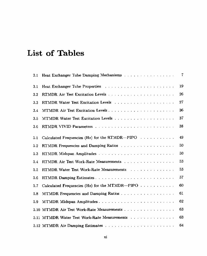
List of Tables
2.1 Heat Exchanger Tube Darnping Mechanisms . . . . . . . . . . . . . . . . 7
. . . . . . . . . . . . . . . . . . . . . . 3.1 Heat Exchanger Tube Properties 19
. . . . . . . . . . . . . . . . . . . . . 3.2 RTMDRAirTest ExcitationLevels 26
. . . . . . . . . . . . . . . . . . . 3.3 RTMDR Water Test Excitation Levels 27
. . . . . . . . . . . . . . . . . . . . . 3.4 MTMDR Air Test Excitation Levels 36
. . . . . . . . . . . . . . . . . . . . 3 5 MTMDR Water Test Excitation Levels 37
. . . . . . . . . . . . . . . . . . . . . . . . . 3.6 RTMDR VIVID Parameters 38
. . . . . . . . . . . 5 Calculated Frequencies (Hz) for the RTMDR-PIPO 49
. . . . . . . . . . . . . . . . . 5.2 RTMDR Frequencies and Darnping Ratios 50
. . . . . . . . . . . . . . . . . . . . . . . . 5.3 RTYDR -Midspan Amplitudes 50
. . . . . . . . . . . . . . . . 5.4 RTMDR Air Test Work-Rate Measurements 53
- . . . . . . . . . . . . . . . a . a RTMDR Water Test Work-Rate Measurements 53
. . . . . . . . . . . . . . . . . . . . . . . . . 5.6 RTMDR Damping Estimates 57
. . . . . . . . . . . 5.7 Calculated Frequencies (Hz) for the MTMDR-PIPO 60
. . . . . . . . . . . . . . . . . 5.8 *MTMDR Frequencies and Darnping Ratios 61
. . . . . . . . . . . . . . . . . . . . . . . . 5.9 MTMDR Midspan Amplitudes 62
. . . . . . . . . . . . . . . . 5.10 MTMDR Air Test Work-Rate Measurements 63
. . . . . . . . . . . . . . 5-11 MTMDR Water Test Work-Rate Measurements 63
. . . . . . . . . . . . . . . . . . . . . . 5.12 MTMDR Air Damping Estirnates 64

. . . . . . . . . . . . . . . . . . . . 5.13 MTMDR Water Darnping Estimates 63
5.14 MTMDR Water Parameters a s a Function of Temperature . . . . . . . . 65
. . . . . . . . . . . . . . . . 3.15 Viscous Damping in Water for the RTMDR 66
. . . . . . . . . . . . . . . . . . . . . . . . . .4.1 .I nalog Input Characteristics 95
A.2 Input Signal Ranges . . . . . . . . . . . . . . . . . . . . . . . . . . . . . 95
. . . . . . . . . . . . . . . . . . . . . . . . . . . .4.3 Tramfer Characteristics 96
A.4 Amplifier Characteristics . . . . . . . . . . . . . . . . . . . . . . . . . . . 96
. . . . . . . . . . . . . . . . . A.5 Amplifier Common-Mode Rejection Ratio 96
A.6 Dlnamic Characteristics . . . . . . . . . . . . . . . . . . . . . . . . . . . 97
. . . . . . . . . . . . . . . . . . . . . . . . . . . . X.7 Dynamic System Noise 97

List of Figures
. . . . . . . . . . . . . . . . . . . . . . . . 3.1 RTMDR Experimental Setup 20
. . . . . . . . . . . . . . . . . . . . 3.2 RTMDR Brass Drilled-Hole Support 21
. . . . . . . . . . . . . . . . . . . . . . . 3.3 RSMDR Support Arrangement 22
. . . . . . . . . . . . . . . . . . . . . . . 3.4 RShIDRMidspanhangement 23
. . . . . . . . . . . . . . . . . . . . 3.5 Shaker and Attacbments (Assembled) 24
. . . . . . . . . . . . . . . . . . 3.6 Shaker and At tachments (Disassembled) 28
. . . . . . . . . . . . . . . . 3.7 RTMDR Shaker Pass-Through Connections 25
. . . . . . . . . . . . . . . . . . 3.8 Top View of MTMDR Support Structure 28
. . . . . . . . . . . . . . . . . . . . . . . . . . . . 3.9 MTMDR Overail View 29
. . . . . . . . . . . . . . . . . . . . . . . 3.10 MTMDR Support Arrangement 31
. . . . . . . . . . . . . . . . . . . . . . . 3.11 MTMDR -Midspan Arrangement 32
3.12 MTMDR Shaker Attachment . . . . . . . . . . . . . . . . . . . . . . . . 33
3.13 MTMDR Heater Locations . . . . . . . . . . . . . . . . . . . . . . . . . . 34
. . . . . . . . . . . . 4.1 Hierarchy of LabVIEW Vibration Anaiysis Program 43
5 . l Sample VIVID Output-Frequency Response Spectrum . . . . . . . . . . 51
5.2 Sarnple VIVID Output-Spectral Peak Curve-Fit . . . . . . . . . . . . . 52
. . . . . . . . . . . . . . . . 5.3 Sample WAVI Output-Support Work-Rate 54
. . . . . . . . . . . . . . . . . . 5.4 Sample WAVI Output-Shaker Input Energy a3
xiii

6.1 RTMDR Air Test Indicating Broad Frequency Response a t Top Midspan-
VNID Result . . . . . . . . . . . . . . . . . . . . . . . . . . . . . . . . .
6.2 RTMDR Air Test 12 Ha Peak at Middle Midspan-VIVID Result . . . .
6.3 RTMDR -4ir Test 30 Hz Peak Growing wi t h Increased Excitation at Middle
Midspan-VTVlD Result . . . . . . . . . . . . . . . . . . . . . . . . . . .
6.4 RTMDR Water Test with Broad Frequency Response a t Top Midspan-
VIVID Result . . . . . . . . . . . . . . . . . . . . . . . . . . . . . . . . .
6 . 5 RTMDR Water Test 24 Hz Peak at Middle Midspan-VD?D Result . . .
6.6 MTMDR .4 ir Test 44 Hz Peak-VNID Result . . . . . . . . . . . . . . .
6.7 Sample RTMDR Air Damping Ratio-VTVID Result . . . . . . . . . . .
6.8 Sample RTMDR Water Damping Ratio-VIVID Result . . . . . . . . . .
6.9 RTMDR Air Test Damping Ratios . . . . . . . . . . . . . . . . . . . . .
6.10 RTM DR Water Test Damping Ratios . . . . . . . . . . . . . . . . . . . .
6.11 MTMDR Air Test Damping Ratios . . . . . . . . . . . . . . . . . . . . .
6.12 MTMDR Water a t 25' Test Damping Ratios . . . . . . . . . . . . . . . .
6.13 MTMDR Water at 60" Test Damping Ratios . . . . . . . . . . . . . . . .
6.14 MTMDR Water at 90" Test Damping Ratios . . . . . . . . . . . . . . . .
6.15 RTMDR Air Test Energy Balance . . . . . . . . . . . . . . . . . . . . . .
6-16 RTMDR Water Test Energy Balance . . . . . . . . . . . . . . . . . . . .
6.17 MTMDR Air Test Energy Balance . . . . . . . . . . . . . . . . . . . . .
6.18 YTMDR Water Test (25' C) Energy Balance . . . . . . . . . . . . . . .
6.19 MTMDR Water Test (60" C) Energy Balance . . . . . . . . . . . . . . .
6.20 MTMDR Water Test (90" C) Energy Balance . . . . . . . . . . . . . . .
. . . . . . . . . . . . . . B . 1 Damping ratio substructure hierarchy of VIVID 100
C.1 Force and Displacement Transducer Layout . . . . . . . . . . . . . . . . . 104

Chapter 1
Introduction
Nuclear reactors contain shell-and-t ube heat exchangers. As t heir name indicates, t hese
heat exchangers comprise a large outer shell housing many tubes. These tubes are s u p
ported at intervals along their length. These supports must be designed so that clearances
around the tubes are sufficient for assembly and thermal expansion.
Thermal energy transfer occurs in heat exchangers by forcing a fluid through the
tubes and another fluid (or fluid-gas mixture) across the tubes. This cross-flow induces
tube vibration. If the vibration amplitudes are too large, damage or even failure can
occur. Failure is due to mechanisms such as fatigue (progressive fractures at areas of
high local stress caused by tube deflection) or fretting-wear (wear caused by relative
motion between the tube and the support while in contact).
Large vibration amplitudes occur due to several phenornena such as vortex shedding,
turbulent excitation, or fluidelastic instability. A flow-induced vibration analysis of a
heat exchanger at the design stage must therefore include these phenornena. To do this,
darnping must be understood.

CHAPTER 1. INTRODUCTION
1.1 Problem
There are three main components of damping for multispan heat exchanger tubes in fluid:
viscous damping along the tube length, friction and squeeze-film darnping a t the supports.
Viscous tube-tefiuid damping is well understood and formulae for its calculation are
availablel. Friction and squeeze-film damping, however, are poorly understood and not
so easily estimated.
1.1.1 Measuring Damping
Two known methods of measuring darnping are the logarit hmic-decrement met hod and
the frequency response curve fit method2. -4 problem common to these methods is
that they require time decay signals or vibration amplitude response peaks that can
be reasonably approximated by ideal functions. Data that are not easily approximated
by these functions do not yield reliable measurements of damping. h o t h e r method of
rneasuring damping would be useful.
1.1.2 The Effect of Temperature on Damping
Heat exchmgers often operate with two-phase water-steam mixtures at temperatures
greater than 250°C. However, much of the expenmental damping work has been done
at room temperature. Results from such experiments may not be adequate in al1 situ-
ations since damping depends on fluid viscosity, and viscosity varies with temperature.
Information about how temperature affects damping would be useful.
' These formulae are discussed in Subsection 2.2.2. *These methods are describeci in Section 2.3.

1.2 Approach
-4 heat exchanger tube vibrates due to the energy it receives from turbulent cross-flow and
other vibration excitation mechanisrns. The tube does not store any of the transferred
energ-y, and so this energy must be dissipated through the available damping mechanisms.
The rate of energy dissipation must be related to the amount of damping in the system.
This thesis marks the first known time that this energy approach was used to estimate
damping.
Chapter 2 reviews the theory and the published experimental results for the two main
areas of interest: damping mechanisms of heat exchanger tubes and heat exchanger tube
work-rates.
Chapter 3 describes the two experimental rigs used for this work. Concepts that
governed the design of one rig are discussed. Data analysis rnethodology is also described.
Chapter 4 describes the three computer programs used to analyze the experimental
data. Special attention is given to the two programs which were developed for this thesis.
Chapter 5 contains the results of the data collection and analysis with the programs
described in Chapter 4.
Chapter 6 discusses the results of the data analysis.
Chapter 7 discusses what this study has accomplished.
The Appendices to this thesis contain information about the computer hardware and
software utilized in this study.

Chapter 2
Literature Review and Theory
Two concepts require review. One is damping, or the energy dissipated by a system. The
other is work-rate, or rate of mechanical energy transfer.
This chapter begins with a section that describes the types of motions observed for
tubes within their supports. Following this are two sections: one on damping ratios
and another on methods for measuring them. The chapter concludes with a section on
work-rates. That section includes a proposal for estimating heat exchanger tube darnping
ratios using an energy balance approach.
2.1 Tube-Support Configurations
When heat eirchangers are assembled, tubes are inserted into holes in baffle-plates or
anti-vibration bars are placed between the tubes. Clearance between the tubes and their
supports is necessary for assernbly and maintenance. No special attempt is made to
center tubes in t heir supports (centering is impossible in horizontal heat exchangers).
Most heat exchanger tube vibration analysis programs simplie calculations by a s
suming that there is always a solid contact between a tube and its support (i.e., a cir-
cumferentially pinned support condition). Ln practice, several different tube-support
configurations may exist :

CHAPTER 2. LITERATURE REVIEW AND THEORY w
3
0 Centered, when the tube and the support are perfectly aligned dong the support
lengt h (nearly impossible to achieve) .
0 Eccentnc, when the tube is closer to one side of the support than the other.
0 Impacting, when the tube rests touching the inside support surface and frequently
impacts on the support when it vibrates. A variation of impacting is contacting,
when a tube touches the support but does not 'lift off' from the surface.
O Sliding, when the tube slides around the inside support surface.
O Scuflng: when the tube simultaneously impacts and slides on the inside support
surface.
Real tu be-support interaction is a complex-and often random-combinat ion of t hese
configurations. These configurations are illust rated in Figure 2.1.
Centered Eccen t ric Impacting Sliding Scuffing
Figure 2.1: Tube/Support Configurations
When a tube impacts, slides, or scuffs in a support (Le., there is significant contact)
that support is said to be effective. An effective support is one that acts like a pinned
support. m e n a tube is centered or eccentnc in a support and vibration amplitudes
are small the tube may contact the support infrequently or not at all. In this case, the
support condition is said to be ineffective. Ineffectively supported tubes no longer behave
as though d l spans are pinned at each end. Analyses that assume they are effectively
pinned will be in error.

2.2 Damping
There are different ways of e-pressing the amount of damping, or rate of energy dissi-
pation, in a system. When damping is quantified, this thesis will use the dampang ratio
which is the ratio of the actual damping coefficient to the critical damping coefficient of
a system.
2.2.1 Energy Dissipation Mechanisms
The annular gaps between heat exchanger tubes and their supports are too large to model
the tube-support interaction with lubrication theory (which neglects fluid inertia) and
too small to allow ideal flow modeling (which neglects fluid viscosity). It is therefore
necessary tu understand the forces and effective mass and darnping associated with the
fluid-filled annular gaps. hlulcahy (11 derived approximate expressions for the fluid forces,
lumped added-mas, and linear damping of tubes in annular regions such as a drilled-hole
support. Mulcahy used t hese approximations to predict the fundamental frequency and
damping of a single beam for the following conditions:
a small fluid motions
finite-length open-ended annular regions
gapteradius ratio << 1.0
viscous penetration of the order of gap width
Rogers et al. [2] reviewed this and other literature for heat exchanger tube-fluid effects.
This review included effects that occur dong the tube and effects that occur within the
clearance between each tube and support. After developing models for added-rnass and
fluid damping, Rogers et al. concluded that the added-mass formula by Mulcahy is
acceptable. They also found that more accuracy is required to properly model squeeze-

CHAPTER 2. LITERATURE REVIEW AND THEORY 7
film damping for al1 except very small tube motions. Both the Mulcahy and Wamer-
Sommerfeld [3] models are reliable for very small motions.
To improve that damping ruodel, Pettigrew et al. [4] outlined several damping mech-
anisms t hat occur in heat exchanger tu be-support interactions. Those mechanisms are
listed in Table 2.1.
Table 2.1: Heat Exchanger Tube Damping Mechanisms
1 Type of Damping 1 Source
1 Structural
Viscous
Flow-dependent
Squeeze-film
Friction
Tuwphase
Intemal to tube material
Be tween fluid forces and forces transferred t O tube
Varies with flow velocity
Between tube and fiuid as it approaches support
Coulomb damping at support
Due to liquid/gas mixture
Damping In Gases
-4fter a review of existing experimental results Pettigrew et al. [5] created guidelines for
the design of heat exchanger tubes in gases. Pettigrew et al. concluded that fiction
damping was the most significant type of damping in gases. Therefore the number
of supports and support length are the m a t important damping parameters in gases.
Diarnetral clearance between tube and support is far l e s important. Parameters such as
frequency, mass, and diameter appear to have no dominant effect o n damping in gas.
Damping In Liquids
Pettigrew et al. [6] also made recommendations for the design of heat exchanger tubes
in liquids. A large amount of damping data from various sources were considered. The
CHAPTER 2. LITERATURE ~ V I E W AND THEORY 8
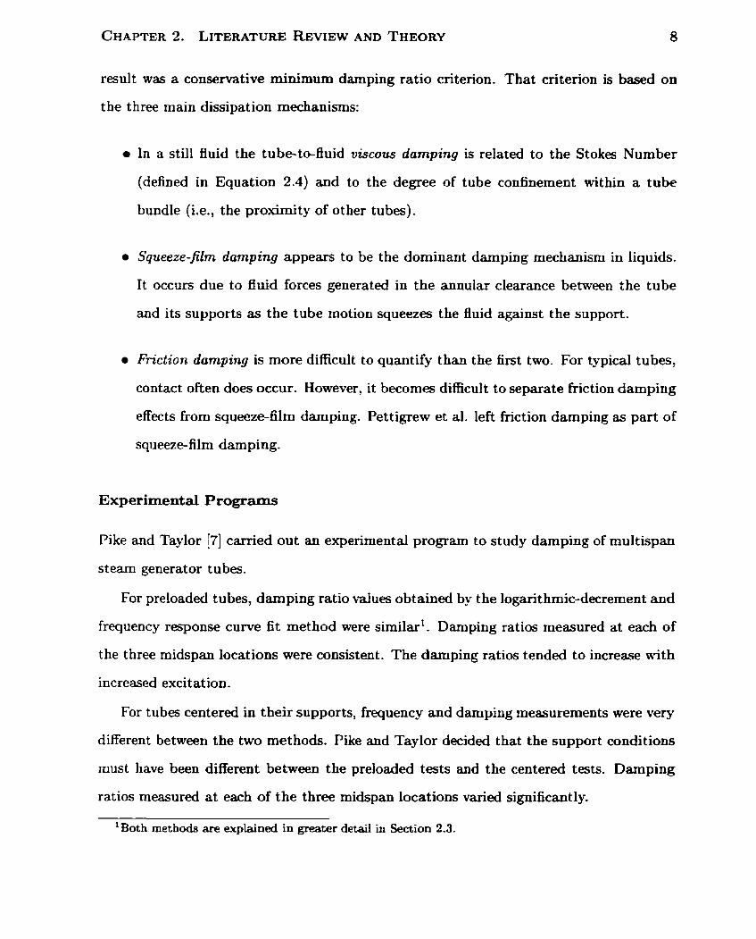
result was a conservative minimum damping ratio criterion. That criterion is based on
the t hree main dissipation mechanisms:
a In a still fluid the tube-to-fluid viscous damping is related to the Stokes Number
(defined in Equation 2.4) and to the degree of tube confinement within a tube
bundle (i.e., the proximity of other tubes).
Squeeze-film damping appears to be the dominant damping mechanism in liquids.
It occurs due to fluid forces generated in the annular clearance between the tube
and its supports as the tube motion squeezes the fluid against the support.
Friction damping is more difficult to quantify than the first two. For typical tubes,
contact often does occur. However, it becomes difficult to separate fiction damping
effects from squeeze-film damping. Pettigrew et al. left friction damping as part of
squeeze-film damping.
Experimental Programs
Pike and Taylor [7] carried out an experimental program to study damping of multispan
steam generator tubes.
For preloaded tubes, damping ratio values obtained by the logarithmic-decrement and
frequency response curve fit method were similarL. Damping ratios measured at each of
the three midspan locations were consistent. The damping ratios tended to increase ~ 4 t h
increased excitation.
For tubes centered in their supports, frequency and damping measurements were very
different between the two methods. Pike and Taylor decided that the support conditions
must have been different between the preloaded tests and the centered tests. Damping
ratios measured at each of the three midspan locations varied significantly.
'Both methods are explaincd in greater d e t d in Section 2.3.
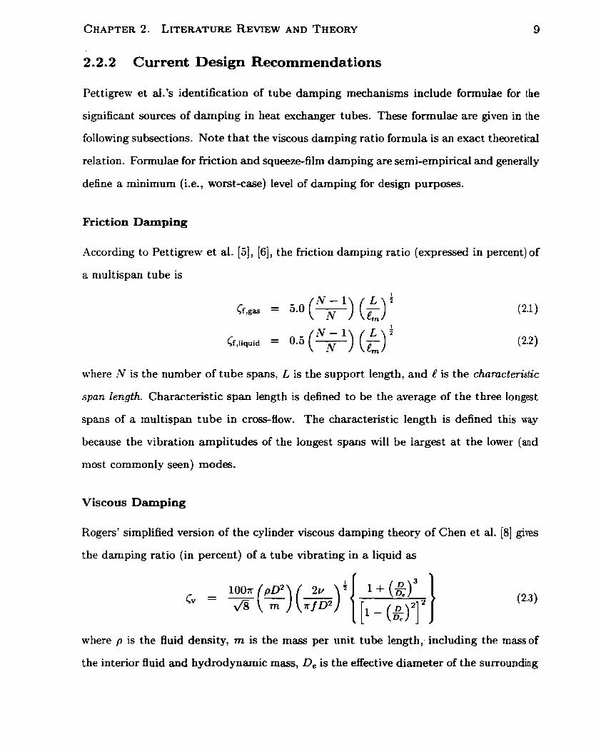
2.2.2 Current Design Recommendat ions
Pettigrew et d.'s identification of tube damping mechanisms include formulae for the
significant sources of damping in heat exchanger tubes. These formulae are given in the
following subsections. Note that the viscous damping ratio formula is an exact theoretical
relation. Formulae for f ic t ion and squeeze-film damping are serni-empiricd and generally
define a minimum (Le., worst-case) level of damping for design purposes.
Friction Damping
According to Pettigrew et al. [5] , [6j, the friction damping ratio (expressed in percent) of
a multispan tube is
N - 1 1
k g a s = 5.0(7) ( f) '
where !V is the number of tube spans, L is the support length, and l? is the characteristic
span length. Characteristic span length is defined to be the average of the three longest
spans of a multispan tube in cross-flow. The characteristic length is defined this way
because the vibration amplitudes of the longest spans will be largest a t the lower (and
rnost commonly seen) modes.
Viscous Damping
Rogers' simplified version of the cylinder viscous damping theory of Chen et al. [8] gives
the darnping ratio (in percent) of a tube vibrating in a liquid as
l - (a)'] where p is the fluid density, rn is the mass per unit tube length, including the mass of
the interior fluid and hydrodynamic rnass, De is the effective diameter of the surrounding
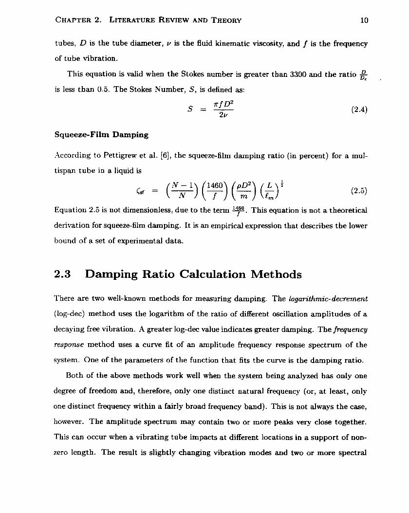
CHAPTER 2. LITERATURE REVIEW AND THEORY 10
tubes, D is the tube diameter, v is the fluid kinematic viscosity, and f is the kequency
of tube vibration.
n This equation is valid when the Stokes number is greater than 3300 and the ratio D;
is less than O.S. The Stokes Number, S, is defined as:
Squeeze-Film Damping
According to Pettigrew et al. [6 ] , the squeeze-film damping ratio (in percent) for a mul-
tispan tube in a liquid is
Equation 2.5 is not dimensionless, due to the term y. This equation
derivation for squeeze-film damping. It is an ernpincal expression that
bound of a set of experimental data.
is not a theoretical
describes the lower
2.3 Damping Ratio Calculat ion Met hods
There are two well-known methods for measuring damping. The logarithrnic-decrement
(log-dec) method uses the logarithm of the ratio of different oscillation amplitudes of a
decaying fiee vibration. A greater log-dec value indicates greater damping. The frequency
response method uses a curve fit of an amplitude fiequency response spectrum of the
system. One of the parameters of the function that fits the curve is the damping ratio.
Both of the above methods work well when the system being analyzed has only one
degree of freedom and, therefore, only one distinct natural fiequency (or, at least, only
one distinct frequency within a fairly broad frequency band). This is not dways the case,
however. The amplitude spectrum may contain two or more peaks very close together.
This can occur when a vibrating tube impacts at different locations in a support of non-
zero length. The result is slightly changing vibration modes and two or more spectral

CHAPTER 2. LITERATURE REVIEW AND THEORY 11
peaks. Mu1 tiple peaks can also occur when the material properties of a system are slightly
different in one direction than in another.
The evperiments done for this work used real tubes of typical rnatenals and supports.
Adjacent spectral peaks did occur. Only one of the above methods of damping ratio
calculation can be made to account for two peaks: curve-fitting the frequency response
spectrum.
2.3.1 Curve Fitting
A best-fit characteristic equation can be applied to experirnent al amplitude spectrum
data. The parameters of the resultant fitted equation are the natural frequency: the
static deflection (also called the zerdiequency amplitude), and the damping ratio. If
there is only one spectral peak, a Iinear least-squares numencal regression method will
provide the parameters. If there are two peaks, a non-linear least-squares method must
be used.
2.3.2 The Marquardt Method
Data is often categorized by fitting it to a mode1 of adjustable parameters. The mode1
may be some convenient hinction or may be constrained by a suspecteci underlying theory.
In most cases this is done by using a ment function that measures the agreement
between the data and the model with a particular set of parameters. If the ment hinction
is arranged so that small values represent good agreement-as is usually the case-the
model parameters are adjusted to minimize the ment function. Parameters that achieve
the minimum ment function (or that decrease the merit function to an acceptable level)
are called the best-fit parumeters.
Met hods for solving a linear least-squares problem are well-documented . The problem
here is curve-fitting two adjacent peaks in a frequency response function. A non-linear
method must be used to solve for al1 the parameters.

CHAPTER 2. LITERATURE REVIEW AND THEORY 12
Mast orakos [9] out lined a procedure using a least-squares estimation of non-linear
parameters developed by Marquardt [IO].
m e n the model depends nonlinearly on a set of M unknown parameters ak, k =
1,2 , . . . , M, the same merit function-minimization approach is used as for the linear
case. The minimization must be done iteratively by improving parameter values until
the meri t function effect ively stops decreasing.
The Marquardt method is generally accepted as an elegant, robust, non-linear regres-
sion model. It has become the standard in non-linear least-squares routines [Il]. It is
used here to fit the frequency response spectra functions of the midspan amplitude data.
The data can be fitted by an equation of the form:
where x are independent variables and P are constant parameters of the function. A
satisfactory solution is found by determining the best estimates, Pm, of the parameters,
P? to minimize the following equation:
n
Residual = (Y, - Y;')
Here. are dependent variables, KA are the amplitudes calculated from Equation 2.6,
and n is the total number of data points. Marquardt's procedure determines corrections
to applÿ to the estimated parameters Pm at each iteration by solving the following equa-
tion:
In this,

CHAPTER 2. LITERATURE REVIEW AND THEORY 13
where [SI is a vector of small corrections applied to each parameter, [Il is the identity
matrix, p is the number of parameters, and A is a convergence parameter.
Initially,. the user must supply guesses for each parameter. The method calculates
corrected estimates after each iteration, k, through the equation:
An iteration is complete when
where r is an arbitrary convergence critenon.
2.3.3 Application to TwePeak Damping Ratios
To measure the darnping ratio parameter using the Marquardt method, the fr
response function that describes the amplitude spect mm is required.
For one spectral peak the function is:
V
For two adjacent peaks:
where Xo is the amplitude a t f = O (the static deflection), f, is the natural frequency
and C is the damping ratio.
Each of these cases has only one independent variable: f . For one peak there are
three parameters: fni , and Ci. For two peaks there are six parameters: &,i, fni , Ci,
IO,2, fn2 and G-
CHAPTER 2. LITERATURE REVIEW AND THEORY 14
In the one-peak case, the equation can be rearranged to isolate each parameter to
obtain the solution. This is not possible in the two-peak case, and so the Marquardt
method is used.
2.3.4 Difficulties with these Methods
The aforementioned methods-log-dec and curve-fitting peaks on a frequency response
plot-are accurate when the time or fiequency signal to be analyzed is distinct. That
is. if a tube vibrates only (or mainly) at one frequency, these methods work well. It has
also been shown that the frequency response curve-fit method can be extended to two
adjacent peaks (representing a tube that is vibrating at two close fkequencies).
Both methods lose accuracy, however, when the support conditions and the vibration
modes becorne more dynarnic. Tube/support interaction can produce very non-linear
behaviour that is characterized by a "cluster" of close frequencies. In a frequency response
function these appear as a very broad single peak. A damping ratio calculated frorn a fit
of this broad peak would not be accurate.
This was a reason for considering an energy approach. Balancing the total energy d i s
sipated by tube motion does not require an understanding of how the support conditions
change. If the approach proves successful, the difficulties of dealing with non-linearities
will be greatly reduced.
2.4 Work-Rates
Work-rate denotes a mechanical energy exchange that takes place a t a particular average
rate. The quantity is therefore more properly defined as power. However, the term work-
rate has been comrnonly used in the fretting-wear study of heat exchanger tubes. The
term is used here as well.
In fretting-wear studies, work-rate is defined as the rate of energy dissipation as a

CHAPTER 2. LITERATURE REVIEW AND THEORY 15
tube in contact with its support moves circumferentially [12]. This relation is described
by the equation
- = - ,IV ' J ~ d s dt t
where T,V is the work-rate, t is time, F is the normal contact force, and s is the sliding
distance. A force (the contact force between tube and support) multiplied by a dis-
placement (as the tube slides) results in work. .4lthough these vectors are orthogonal,
fretting-wear studies have shown that the material damage rate is closely related to the
normal forces during contact.
Pike and Taylor attempted to measure work-rates in their experiments2. Tub+
support impacts were of insufficient magnitude to measure work-rates, however. Pike
and Taylor concluded that for the tests where the tube was centered the tube never
achieved large enough motions. For their preloaded tests they concluded that the tube
never received sufficient excitation lettels to lift off from the support.
2.4.1 Work-Rates as Damping Ratio Estimators
Damping is a measure of the rate of energy transfer. Relating work-rate to damping
seems reasonable. This rnight result in another method of estimating the damping if two
equations are met:
1. reliable work-rate measurements that can be associated with the rate of energy loss
of a system can be made, and
2. the damping measured with a work-rate method agrees with that estimated with
known methods.
It is assumed that a multispan tube can be simplified to three single-span simply-
supported tubes. For a simple one-degree-of-freedom system comprising a spring, mass,
'Sec Subsection 2.2.1.

CHAPTER 2. LITERATURE REVIEW AND THEORY 16
and viscous damping, the harmonic displacement and velocity are defined as follows:
x = ,y sin (2n f t - 6)
According to Thomson [13j, the energy dissipated per cycle of vibration at resonance,
Wd, for this system is
ahere n~ is the equivalent mas , C is the damping ratio, f, is the natural frequency, and
S is the peak amplitude of vibration.
From Equation 2.7, the equivalent viscous damping is estimated by
The equivalent mass for the tube is calculated from
m = J M(x)@* (x) dx tube tength
where M ( x ) is the mass of the tube plus the added interior water and hydrodynamic
mass per unit length of tube, and +(x) is the mode shape of the tube. If the tube mode
shape is being approximated by a sinusoidal function then @(x) = sin (xx/t?) . In this
equation, x is the vertical location dong the span, and l is the length of the span.
Calculating the energy dissipated in this way requires the peak vibration amplitudes.
The excitation of heat exchanger tubes by turbulence is random. The peak amplitude
of a zero-mean random signal may be assurned to be three times the standard deviation
(equivalent to the RUS) value, since approximately 99.7% of the random amplitudes
will fall within that limit. Equation 2.8 is for sinusoidal vibration, however-a peak
amplitude for this motion would be times the RUS value. As an approximation, and
since rig components surrounding the tube may constrain vibration, a peak amplitude of
vibration of twice the RUS value will be assumed.
CHAPTER 2. LITERATURE REVIEW AND THEORY 17
Knowing the shaker power transferred to the tube, and assuming a one-degree-of-
freedorn vibration, an equivalent damping ratio can be calculated. In this case the as-
sumed amplitude of vibration is the average amplitude of the three spans. The effective
mass is the sum of the m a s of the three spans.
It bears repeating that, at the time of this work, this energy approach to estimating
damping had not been attempted. It is also worthwhile to note that since this work
was completed more use has been made of this method. Results published by Taylor
et al. [14] used the equipment and analysis programs developed for this study to test
heat exchanger tubes under different support pre-load conditions. These results, and the
energy method for estimating damping that was used, were reviewed by Pettigrew et
al [l 51. They were also used by Yetisir et al. [16] in the development of an operational
hea t-exchanger specification based on work-rate.

Chapter 3
Experimental Procedure
Two sets of experiments were completed for this work. The first set is from the orig-
inal room-temperature muitispan damping rig and is discussed in Section 3.1. These
e~periments provide results that act as a baseline for the design and edua t ion of a
higher-temperature rig. The second set of experiments are from the newly-constmcted
mid-temperature multispan damping rig. These experiments are discussed in Section 3.2.
These experirnents provide more data points in the investigation of the effect of tem-
perature on damping. These data may serve as an indicator of whether further high-
temperature damping experimentation is necessary.
3.1 Room-Temperat ure Multispan Damping Rig (RT-
MDR)
The Room-Temperature Multispan Damping Rig (RTYDR) was constructed several
years before this testing was begun. I t was used for many sets of experiments in the
Vibration and Tribology Unit (VTU) of Atomic Energy of Canada Limited. In that
time, the RTMDR underwent significant adaptations and evolutions.

3.1.1 Construction and Instrumentation
The RTMDR is essentially a heat exchanger tube in a stainless steel trough. The rig-
originally used horizontally-stands vertically to an overall height of about 4 m. The
trough has three sides. The front is opened and shut with a swinging door lid. The
trough is open to the atmosphere at the top. A picture of the RTMDR is shown in
Figure 3.1.
Inside the RTMDR trough are two long vertical plates attached to the back of the
trough. These plates are supported at intervais with fins and bars that attach to the
trough sides. -Mdspan and support platforms fasten to these two vertical plates. The
platforms may be moved and Lxed at any location dong the tube. Changing the support
platform locations &anges the lengths of the tube spans.
The RTMDR heat exchanger tube properties are shown in Table 3.1. Each RT'VIDR
tube span length is 1.219 m.
Table 3.1 : Heat Exchanger Tube Properties
Material
Inner diameter
Outer diameter
Free length
Densi ty
There are six platforms along the tube a t even intervals. Each platform has transducer
assemblies. Three platforms have b r a s drillecl-hole supports (see Figure 3.2). Support
platforms are instrumented with two eddy-current displacement probes-aimed at a tar-
get ring on the tube and positioned 90" apart-and a ring with four piezoelectric force
transducers. The force transducer ring is in contact with the support. .4ny contact force

- f --- ci. - . 7- 1 i :? - * - Y . "
. .. [?a ,-' :,ki g ; E 9--
Figure 3.1: RTMDR Expenmental Setup. The front face of the trough rig (right) is a
Plexiglas lid. The tube can be seen in the centre of the trough as can several of the
support and midspan transducer platforms. The shaker platform is near the top of the
trough (shakers not shown). Sensor signal wires leave through the right side of the trough.
Excitation, measurement, and recording instruments are shown (left ) .

between the tube and the support results in a signal from the force transducers.
By using four force transducers the direction of impact can be determined. Piezo-
electric force sensors only produce positive signais. They emit a charge only when they
are compressed. Opposite-direction force signals at each support are added via summing
boxes. This produces two orthogonal force measurements a t each support. See Figure C.1
for a force ring arrangement diagram.
Figure 3.2: RTMDR Brass Drilled-Hole Support
Three platforms do not bave supports. They have large holes t hat do not interfere wit h
tube movement and are for transducer placement at the midspans only. The arrangement
of support and midspan platforms is shown in Figures 3.3 and 3.4, respectively.
Two vibration generators (shakers) excite the tube. The shakers are clamped to a
steel platfom that is bolted to the trough lid. The input motion signals are supplied by
two random noise generators. These signals are filtered to bandpass frequencies between
1 and 100 Hz.
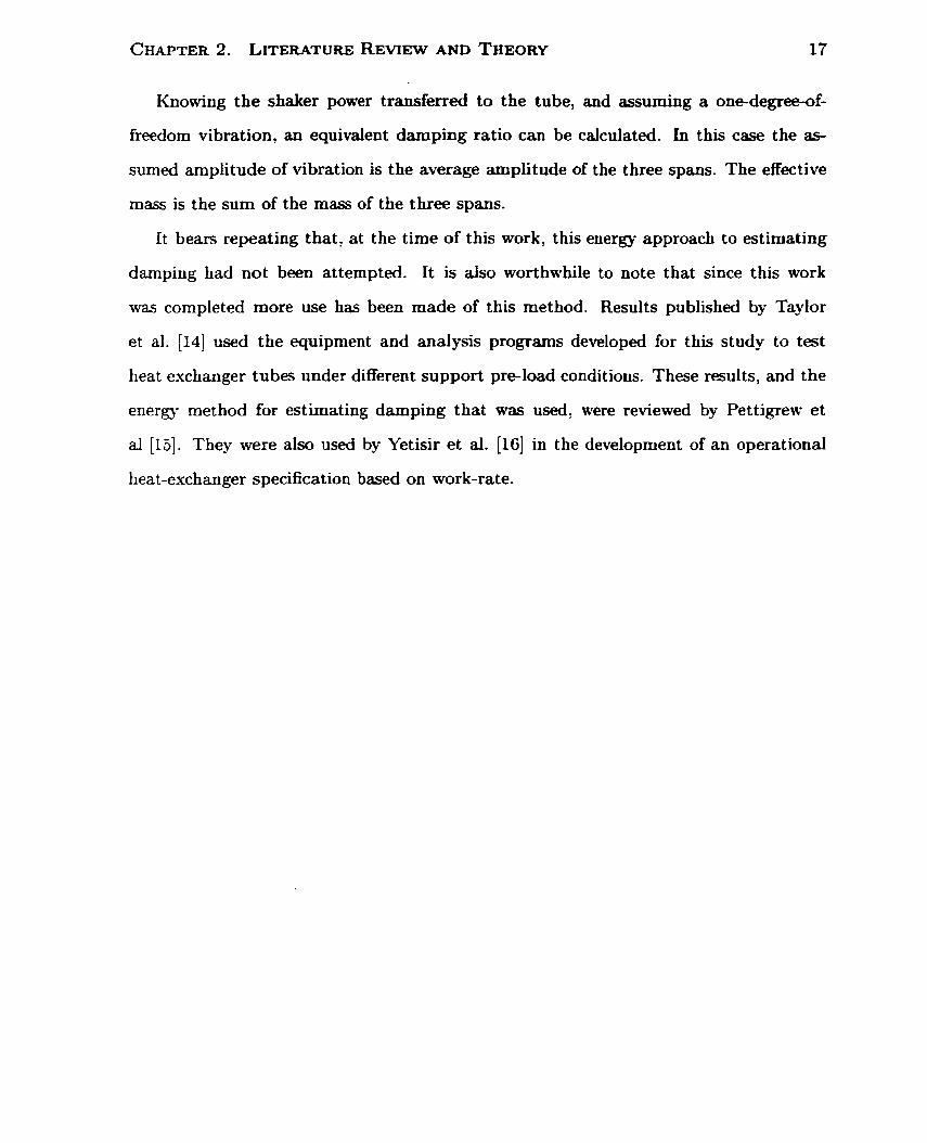
The shakers connect to the tube through a series of attachments. Figure 3.5 shows a
picture of the shaker and assembled attachments. Figure 3.6 shows the same equipment
when disassembled. A threaded rod on the shaker (A) connects to an impedance head
(B). A short rod (C) and a colla (D) with two set-screws provide length adjustability
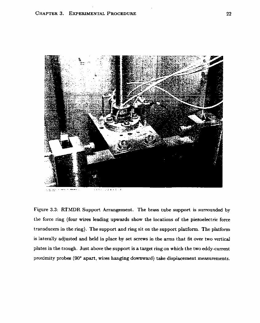
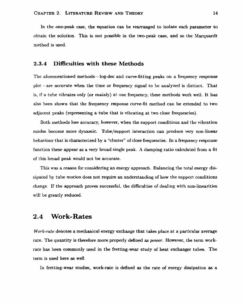
Figure 3.3: RTMDR Support Arrangement. The b r a s tube support is surrounded by
the force ring (four wires leading upwards show the locations of the piezoelectric force
transducers in the ring). The support and ring sit on the support platform. The platform
is laterally adjusted and held in place by set screws in the arms that fit over two vertical
plates in the trough. Just above the support is a target ring on which the two eddy-current
proximity probes (90" apart, wires hanging downward) take displacement measurements.

Figure 3.4: RTMDR Midspan Arrangement. The tube passes through a hole in the
platform. This hole is sized large eaough so that the vibrating tube will not contact it.
The platform is laterally adjusted and held in place by set screws in the arms that fit
over two vertical plates in the trough. There is a target ring at this location on which the
two eddy-current proximity probes (seen 90" apart) take displacement measurements.

to faciIitate installation. The collar fastens to a threaded rod (E) that attaches to a
short section of steel cable with threaded bras ends (F). The cable is needed to align the
shaker rods with the pass-throughs and tube connection. The cable connects to a b r a s
collar that tightly encircles the tube. Shaker attachment through the front lid door to
the tube is shown in Figure 3.7.
.411 test signals were recorded on a VHS cassette magnetic tape recorder.
3.1.2 Operation
The first step was to adjust the support platforms to center the tube in al1 three of its
supports. This proved impossible since the tube-clamped at the bottom and free at al1
supports-is a thin, 3.74 m vertical1 y cantilevered beam. Tube deflection always caused
Figure 3.5: Shaker and At tachments (Assembled)
Figure 3.6: Shaker and Attachments (Disassernbled)
Figure 3.7: RTMDR Shaker Pas-Through Connections

contact with the top support. In the end, RTMDR testing was done with only the bottom
support centered.
The next step was to check that al1 force and displacement sensors were operating
properly. This was done before the front lid of the rig was closed, since closure prevents
access to the trough intenor. Once the front lid was closed (and al1 seaiing clamps engaged
for the water tests), the shaker rods were inserted through the pas-throughs and screwed
into the tube collar. The shakers were positioned so that their rods moved heely through
the pass-throughs. The shakers were then clamped down. Rubber diaphragms were
fastened over the pas-throughs and attached to the shaker rods, if water tests were
performed. For water tests, an attached water line valve was opened. This filled the
t rough.
The final step was to set the shaker power level. Signais were recorded to tape while
the tube vibrated for several minutes.
R-MS shaker forces for these tests are shown in Tables 3.2 and 3.3.
Table 3.2: RTMDR Air Test Excitation Levels
Test Level Shaker RMS Force Input Level (N)

Table 3.3: RTMDR Water Test Excitation Levels
1 Test Level 1 Shaker RMS Force Input Level (N) 1
3.2 Mid-Temperature Multispan Damping Rig (MT-
MDR)
Testing in heated water would require substantial structural changes to the RTMDR. A
new experimental rig-the Mid-Temperature Mu1 t ispan Damping Rig (MTMDR)-was
a more effective option.
There were three guidelines for MTMDR design:
1 . Operation must be saje. The multispan damping rig is a ta11 container of heated
water. There must be human operators present during testing. The rig must be
located in an area where other equipment, experiments? and people operate. -4n
operator must be satisfied that there will not be any water spillage.
2. Keep as much original room-temperature rig design as is practical. One reason for
this is that the original RTMDR design has proven to be a simple and workable one.
It was used for many experiments and was adaptable. Another reason is that the
MTMDR can serve as a "stepping-stone" between measurements taken from the
RTMDR and possible future high-temperature multispan damping experiments.
Another reason is that a similar design may allow parts of the RTMDR to be used
in the MTMDR. This minimizes cost and time.
3. There must be a way to heat the water inside the rïg. To investigate the effect of

temperature on damping it must be possible to efficiently, safely, and accurately
heat the water inside the rig.
3.2.1 Construction and Instrumentation
The MTMDR is-like the RTMDR-a single vertical heat exchanger tube clamped at
the bottom and supported at three other equally-spaced locations. The entire rig may
be enclosed so that the tube can be surrounded by water. Two back-to-back vertical
C-shaped channels (see Figure 3.8) provide a frarne for the transducer platfoms. These
channels and the tube clamp bolt to a heavy steel base plate on the floor. An overall
view of the -MTMDR is shown in Figure 3.9.
Support or Midspan Platform
Figure 3.8: Top View of MTMDR Support Structure
The shell enclosing the rig is a stainless steel pipe. It has a bottom flange that is
sealed by an O-ring in the floor baseplate. The shell has several electric heaters attached
to its outside surface, so that water inside the shell can be heated. A layer of insulation
covers tbe shell and heaters. The shell also has two holes at the top so that a Crane may
attach for shell installation and removal. The top of the shell is open to air to permit
tube coupling to the shakers and to provide an easy exit for sensor cables. An open top
also ensures that the inside rig test area cannot become pressurized if water evaporation
OCCUrS.
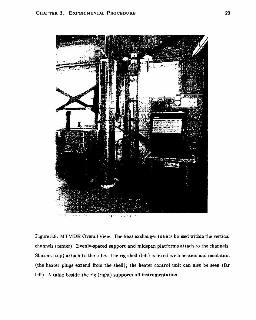
Figure 3.9: MTMDR Overall View. The heat exchanger tube is housed within the vertical
channels (tenter). Evenly-spaced support and midspan platforms attach to the channels.
Shakers (top) attach to the tube. The rig shell (left) is fitted with heaters and insulation
(the heater plugs extend from the shell); the heater control unit can also be seen (far
left). A table beside the rig (right) supports al1 instrumentation.
MTMDR support and midspan platforms are shown in Figures 3.10 and 3.11 respec-
t ively.
The shakers are bolted to a steel plate that is solidly attached to an adjacent interior
wall. The shaker heads at tach to a collar a t the top of the tube (the tube extends several
inches above the top of the shell). Figure 3.12 shows the shakers and how they attach to
the MTMDR tube.
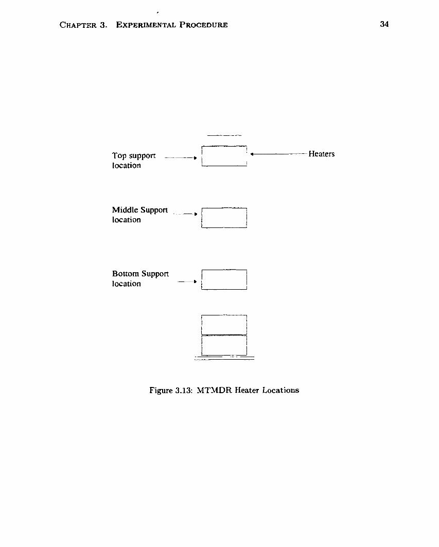
The MTMDR was developed to allow testing in water at higher temperatures. This
was accomplished by attaching five 2500 W electric band heaters to the outside of the
shell that encloses the rig. Figure 3.13 shows the positions of the heaters. Two heaters
are located at the bottom of the shell. This concentrates heat input at the bottom
of the water column when the liquid is initially heated. This warmer water will rise
because of natural convection. The other three heaters are each located at shell positions
corresponding to tube support locations.
.U1 Bve heaters are wired to a control unit located beside the rig (see Figure 3.9). The
two bot tom heaters operate only by on/off switching and are generally used only to heat
the water column to the target temperature. The other three heater temperature levels
are set by manual analog dials on the control unit. Heaters are controlled by feedback
from thermocouples attached to the rig near each heater.
The temperature control system also has a safety feature t hat prevents heater burnout
iri the case of water evaporation. A master control is wired to a safety thermocouple that
is a t t d e d to the interior surface of the shell near the top heater. If the heaters are
inadvertently left a t a setting high enough to cause water evaporation, the liquid water
level could drop enough over time to expose the inside shell surface to air. This would
cause a jump in shell temperature and burnout damage to the shell, heater, or instmmen-
tation. The master control will shut off al1 heaters if it registers a safety thermocouple
temperature greater than 100 O C (indicating that al1 liquid water has evaporated down
to that level).

Figure 3.10: MTMDR Support Arrangement. The support arrangement is similar to the
RTMDR (see Figure 3.3). The support is surrounded by a force ring with four force
sensors. Two motion sensors measure displacement of a target ring.
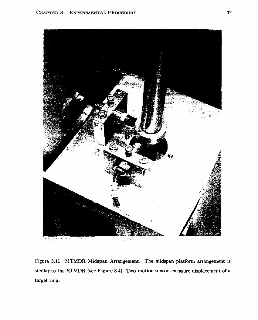
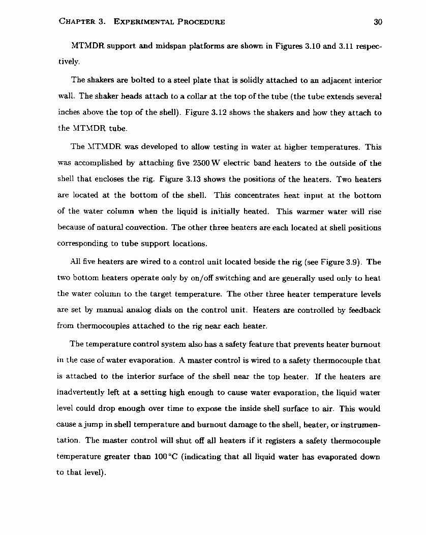
Figure 3.11: MTMDR Midspan Arrangement. The midspan platfom arrangement is
sirnilar to the RTMDR (see Figure 3.4). Two motion sensors measure displacement of a
target ring.

Figure 3.12: MTMDR Shaker Attachment. The shakers attach to a tube collar through
a series of connectors (see Figures 3.5 and 3.6). Two motion sensors (90" apart) on the
top of the rig measure the displacement of the tube just beneath the attachment point.
Shakers receive their input signals via terminais on top of the shaker cylinder. Shaker
force signals and acceleration signals (not used) are measured via outputs on the shaker
impedance head. The shakers are bolted to their platform. The piatform is attacheci to
two vertical supports that are solidly bolted to the wall of the building that houses the
MTYDR. Tiiermocouple leads can also be seen (far left).
Top support --, m. 1 Heaters ! location
Middle Suppon location
J
Bottom Suppon location
Figure 3.13: MT-MDR Heater Locations

Differences Between the RTMDR and MTMDR
Access to the tube and transducers in the RTMDR is limited, since the trough encloses
the tube on three sides. The vertical channels in the MTMDR make access to the tube
and transducers easier, since there are two open sides. In addition, the channels have
holes that allow limited side access.
Sealing the MTMDR for water tests is easier and safer than with the RTMDR. The
RTMDR has a front door lid that is clamped shut. Many locations (such as seams in
the glass plates of the front door) must be regularly re-sealed. The only sealing location
in the MTMDR is where the shell flange m e t s the finished surface of the baseplate. A
groove in the baseplate houses a rubber O-ring that maintains a seal. The flange is held
d o m with eight heavy bolts.
For the RTMDR the shakers are fastened to a platform on the front door of the rig.
The shakers connect to the tube a t the top midspan. For the MTMDR, the shakers
connect with the collar a t the very top of the tube.
Another difference with the MTMDR is that although the same heat exchanger tube
was used, space constraints required shortening the overall tube length. The length of
each span was therefore shortened. The RTMDR had an overall tube length of 3 . 7 4 1 ~ .
In the MTMDR, each span was 0.913m long, for an overall tube length of 3.023 m.
The functional Avantage of the MTMDR over the RTMDR is the ability to test in
water at higher temperatures
3.2.2 Operation
Based on preliminary RTMDR results analyzed at the time of this testing it was decided
that it would be more useful to preload dl three supports for MTMDR testsL. Ail three
'The RTMDR results suggested that support conditions changed with increasing excitation. The bottom sup port--centered before the tests and at low excitation levels-became effective as contact occurred at higher levels. This changed the support conditions from two to three spans during testing.
supports were preloaded by adj us ting the support platforms so that the tube contôcted
them with a force of approximately 2 N.
The following steps are similar to those used for the RTMDR (see Subsection 3.1.2).
Sensor operation was verified before the shell was placed over the rig and bolted down
at the flange. Once the shell was in place shaker rods were connected to the tube collar.
If the test was in water, a nearby water line was inserted into the open top of the
shell and the shell filled. If the test was to be in heated water, the heater control unit
was turned on, the bottom two heaters were tumed on: and the three support heater
controls were set to the desired temperature. Once the support location thermocouples
registered near the target temperature, the bottom two heaters were turned off.
The heater control system provided accurate water temperatures. Thermocouple
measurements indicated that the temperature at any support location never varied by
more than 3°C from the setpoint.
The next step was to tum on the power amplifiers for the shakers and set a power
level. Data was recorded on tape for several minutes.
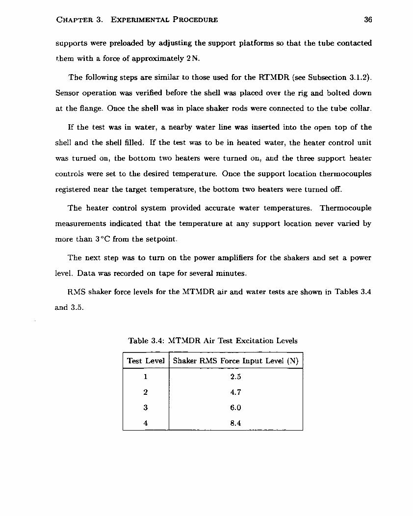
R-MS shaker force levels for the MTMDR air and water tests are shown in Tables 3.4
and 3.5.
Table 3.4: MTMDR Air Test Excitation Levels
1 Test Level 1 Shaker RMS Force Input Level (N) 1

Table 3.5: MTMDR Water Test Excitation Levels
3.3 Data Analysis Method
Test Level
There were four steps to data analysis, descx-ibed in Subsections 3.3.1 through 3.3.4.
Shaker R-MS Force Input Levei (Pi) at
Different Water Temperatures (OC)
3.3.1 Analysis Step 1-Calculate Theoretical Vibration Modes
1 1 25 1 60 1 90
The first step was to calculate vibration frequencies and mode shapes for the test tubes
under diff'erent support conditions. This did not require test data. The computer program
PIPO was used for these calculations (more information on PIPO is given in Section 4.3).
Performing t hese calculations required supplying PIPO wi th information about tube
geometry and support conditions.
3.3.2 Analysis Step 2-Measure Vibration Modes and Damping
The second analysis step was to perform a frequency response analysis of the recorded
tube displacement amplitude data. V M D was the computer program developed to do
this analysis (more information on VIVID is given in Section 4.1).
VIVID acquires time-domain midspan vibration amplitude data from the data tape.
It then uses the Fast Fourier Transform (FFT) method to calculate the frequency con-

tent of that data. Because of the multi-channel acquisition capability of VTVID, all six
midspan displacement signals (two orthogonal directions at each of three midspans for
each test) were simultaneously analyzed. The analysis parameters for the tests are given
in Table 3.6.
Table 3.6: RTMDR VTVID Parameters
Analysis Parameter
(each channel)
Number of windows
Data window
Sampling rate
Data window size
10 or 18
Hanning
RTMDR Tests
35
Hanning
-MTMDR Tests
128 Hz
2048 points
VIVID acquired 16-second windows (data window size divided by sampling rate)
of time-domain data for al1 midspans and performed the FFT calculations n e c e s s q to
obtain a frequency response spectrum. This process of capture and analysis was repeated
for a number of windows. An average resultant response spectrum was calculated.
The analysis parameters used for the RTMDR tests were based on the maximum
available computer mernory. Higher sampling rates or larger windows caused program
execution errors. No significant diasing errors were expected, however. According to the
results of PIP02 the sampling rate of 128 Hz is still greater than twice the frequencies of
the first three modes for any support configurations in air or water.
-4 ten-window average was the largest number possible with the amount of data
recorded. The RTMDR tests were the first done and the duration of test data had to be
estimatéd.
Prior to the MTMDR tests, memory was added to the analysis cornputer. This
'See Table 5.1.
256 Hz
4096 points

allowved the sarnpling rate and window size parameters for the MTMDR test analyses to
be increased. The duration of recorded test data was also increased so that the nurnber
of averages could be increased.
The Hanning window mentioned in Table 3.6 is a digital manipulation of the sampled
signal in an FFT andysis. The window forces the first and last samples of the time
record to zero amplitude. This compensates for an inherent error in the FFT algorithm.
The FFT algorithm assumes that the tirne-domain signal it analyzes is periodic. If the
tirnedumain sample being analyzed does not contain an integral number of cycles, the
periodic cycle of the sample will contain discontinui ties. These discontinui ties cause the
energy at specific frequencies to be "spread out" (spectral leakage).
Damping ratios from amplitude frequency response peaks were calculated for every
displacement signal spectrum with one or more visually distinguishable peaks. If the
prograrn converged on a solution for the damping ratio, the frequency where the peak
occurred and the damping ratio were recorded.
3.3.3 Analysis Step 3-Measure Input Energy and Work-Rates
at Supports, and Estimate Damping
The third step mras to perforrn work-rate measurements from the recorded tube support
forces and motions, and from the shaker input energy. The program developed to do
this-W.4VI-is descnbed in more detail in Section 4.2 and Appendix C.
WAVI simultaneously acquires four channels of time-domain data (two displacements
and two forces). For support work-rates the displacements are of the tube and the forces
are those measured in the sensors around the support. For input power to the tube, the
displacements and forces are those of the random excitation of the shakers.
Al1 tnalysis was done from taped data acquired at 8192Hz (each channel) for a
duration of 1 second. Displays of the orbital path of the acquired displacements (part
of WAVI's results) indicated that this was a sufficient sample length to characterize the

random motion of the tube in its support. WAVI calculated work-rate (or input power)
based on these signals and displayed the results. This 1-second analysis was repeated
at least four times for each support or shaker input. The results for each test condition
were averaged.
A damping ratio was also calculated from the dissipated shaker input energy using
the shaker input power and Equation 2.8.
3.3.4 Analysis Step 4-Calculate Expected Darnping Ratios
The final analysis step was to calculate expected damping ratios from the equations of
Subsection 2.2.2.

Chapter 4
Analysis Tools
Three computer programs were used to collect and analyze the test data: PIPO, VNID
and W.4VI. V M D and WAVI were specially developed for this study. VIVID acquires the
test data: calculates the tube midspan vibration amplitudes, and calculates and plots the
corresponding frequency response spectra. It also calculates darnping by curve-fitting the
spectral peaks. WAVI acquires the test data and calculates the work-rates at the supports
and at the excitation shakers. PIPO was used to calculate the natural frequencies and
the mode shapes of the multispan tubes. These calculations were compared with the
results of VNID.
4.1 Virtual Instrument for Vibration and Int egrated
Damping (VIVID)
Measuring the frequency spectra of multispan tube responses is compu tationally inten-
sive. Analog-tedigital signal conversion and computer programs were used to maximize
analysis efficiency.
LabVIEW is a versatile software tool for data acquisition, analysis, and process con-
troll. When this work was initiated, VTU was in the process of implementing LabVIEW
in several programs. LabVIEW programs were also developed for this study.
4.1.1 Implementation
The main requirements for data analysis were:
a multiple-channel signal input,
a spectral analysis (e.g., Fast Fourier Transform, o r FFT),
a an operational choice to acquire data t hrough analog-to-digi tal (A/ D) conversion
from an extemai source or read a data file of previously acquired and saved results,
a analysis capability to calculate RVS values within variable spectral bandwidths
and to perform spectral data curve fits to estimate system parameters like naturai
frequency and damping ratio, and
0 al1 of the above in an iutegrated program.
LabVIEW programs are called virtuai instruments (VIS) because the user interface
on the computer screen resembles an actual instrument with controls and indicators. -4
VI called as a subroutine from another VI is called a subVI.
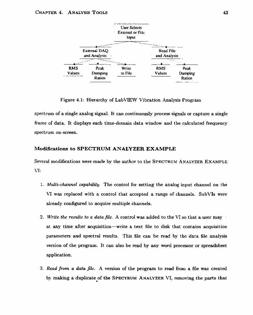
Decisions about how the analysis program should be structured resulted in the hier-
archy s h o w in Figure 4.1.
LabVIEW's structure is modular and hierarchical. Repetitive tasks or distinct levels
of operation separate easily into subVIs. LabVIEW subVIs connect more visibly than do
subroutines in text-based languages, and the hierarchical structure of the entire program
is easily seen.
LabVIEW contains a program named SPECTRUM ANALYZER EXAMPLE that m e t s
some of the requirements. SPECTRUM ANALYZER EXAMPLE cornputes the frequency
'See Appendùc A.
User Selects Externa1 or File
Input
Extemal DAQ R a d File and Analysis and Analysis A/--
<- ----.\_ , - 4 c L - A- - A
RMS Peak Wri tc RMS Peak Values Damping IO File Values Darnping
Ratios Ratios
Figure 4.1: Hierarchy of LabViEMr Vibration Analysis Program
spectrurn of a single analog signal. It can continuously process signals or capture a single
frame of data. It displays each time-domain data window and the calculated frequency
spect rum on-screen.
Modifications to SPECTRUM ANALYZER EXAMPLE
Several modifications were made by the author to the SPECTRUM ANALYZER EXAMPLE
VI:
1 . Multi-channet capubility. The control for setting the analog input channel on the
VI was replaced with a control that accepted a range of channels. SubVIs were
already configured to acquire multiple channels.
2 . Write the results to a data file. A control was added to the VI so that a user may-
at any time after acquisition-write a text file to disk that contains acquisition
parameters and spectral results. This file can be read by the data file analysis
version of the program. It can also be read by any word processor or spreadsheet
application.
3. Read f r o n a data file. A version of the program to read from a file was created
by making a duplicate of the SPECTRUM ANALYZER VI, removing the parts that 9
acquire signals from the DAQ card and replacing them with subVIs to read text
files. The program identifies those lines of the file that are header information and
those that are data points.
4. Calculate RMS values. Root-mean-square values of a signal within a given fre-
quency bandwidth can be measured by taking the square root of the surn of al1
the discrete values of the signal power spectrum within that bandwidth. An R\iS
value within the entire bandwidth is calculated automatically by performing this
operation on every point in the spectrum. Cursors on the amplitude spectrum
graph allow the user to measure the R\iS value for any frequency.
5 . Estimate dumping. VTU uses a FORTRAN code (~PEAK) that uses numericd
iteration to solve the damping equation. This method required acquiring data,
writing it to a file, and then executing PEAK to read the file and output results.
The numerical met hod used (the Marquardt dgorithm for least-squares estimation
of nonlinear parameters') was translateci into equivalent LabVIEW code to be
available as a subVI Erom the main user interface3.
Results
The modifications listed above resulted in Virtual Instrument for Vibration and Inte-
grated Damping, or VIVID. When used with the base LabVIEW for Windows program
and a data acquisition card it accomplishes al1 the acquisition and analysis requirements.
A sample of VIVID output can be seen in Figures 5.1 and 5.2.
2See Subsection 2.3.2. 3See Section B.2 in Appendix B.
4.2 Work-Rate Analysis Virtual Instrument (WAVI)
A work-rate measurement tool was also required. To do this, a method of measuring
work-rates a t tube supports and a t the point of excitation was developed.
4.2.1 Implementation
-4 work-rate analysis computer code already existed in VTU as part of a fretting-wear
program. That code, named Work-Rate Analysis Program (WRAP), is a LabCTEW VI
that measures work-rates from contact between a single heat exchanger tube and its
support. The force and displacement transducer assembly used for the fretting-wear rig
support is the same as that used in both multispan damping rigs. WR4P [vas modified
by the author to create a multispan work-rate measurement program.
Modifications to MrRAP
U r M P was originally developed to run under LabVIEW on a 'ulacintosh computer. The
first step was to translate WRAP to a Windows PC platform. LabVIEW Vis are directly
portable between the two platforms.
WR4P calculates work-rates for a tube in a support with instrumentation identical to
that of the multispan rigs. Little modification was necessary to the calculation portions
of the program. There were three main modifications:
1 . Interactive user-defined contact criterion. When WRAP is used to estimate work-
rate, the program applies a contact criterion to the force data. If a force data point
falls above a certain user-defined level, contact is considered to have occurred. If
the data point falls below that force threshold, it is assumed no contact occurred.
This eliminates noise effects in the force signals. This contact criterion is defined
as a percentage of the maximum force signal. It is input by the user before the
program begins. This requires that the user have an idea of the fom of the force
signal before it is acquired. For WAVI, an interactive program step was included
to display the entire sampled force signal after acquisition. This allows the user to
interactively set a contact criterion level.
2 . VI for shaker work-rates. Since the rate of energy supplied t o the tube by the
shakers is measured, a subVI to measure work-rate from the shakers was developed.
This subVI is similar in f o m to the one that calculates work-rates at the supports.
Here, however, the work-rate calcuiated is the power transfmed fiom the shakers
to the tube.
3. Output fonnat. A different output format was developed for WAVI. Some results
were re-ordered and re-labelled from t heir WR4P format. O t her calculation steps-
such as the force signal after the contact criterion has been applied, and an X-Y
orbital plot of the support or shaker displacement-were included.
Result s
These modifications resulted in the Work-rate Analysis Virtual Instrument, or MT74Vi.
When used with the base LabVIEW for Windows program and a da ta acquisition card
it accomplishes al1 work-rate measurement requirements. A sample of WAVI output can
be seen in Figure 5.3.
4.3 Vibration Analysis Code (PIPO)
PIPO is a modification of the original French word for the code, "Pipeau," meaning,
roughly, "small pipe". PIPO is a VTU computer code for heat exchanger vibration
analysis. It can caiculate natural frequencies, mode shapes, and amplitude response
levels for flow-excited heat exchanger tubes of any configuration. For this study, PIPO
was used to provide analytical values for natural frequencies and mode shapes for each

of the tubes tested. These values were compared with the frequencies measured using
VIVID.

Chapter 5
Result s and Calculat ions
The experimental data is presented in this chapter.
In the first section, RTMDR tube frequencies are calculated using PIPO. This section
also shows how damping is calculated with VIVID. It also contains rneasurements of work-
rates aiid damping estimates made from these measurements. Finally, the simplified
equations of Subsection 2.2.2 are used to calculate the expected total damping.
The second section contains corresponding results from the MTMDR tests.
5.1 RTMDR
5.1.1 Vibration Analysis using PIPO
RTMDR tests were carried out in air and water at room temperature. Since dl : some, or
none of the tube supports may be effective' in any vibrating condition, there are several
possible support configurations. The calculated natural frequency results from PIPO for
the first five modes of vibration at different support conditions are shown in Table 5.1.
Different support conditions are indicated in this table by a graphic representation of
the vertical RTMDR tube and its supports. In each case the tube is shown as effectively
'See Figure 2.1 for the definition of an eftèaive support.
48
CHAPTER 5. RESULTS AND CALCULATIONS 49
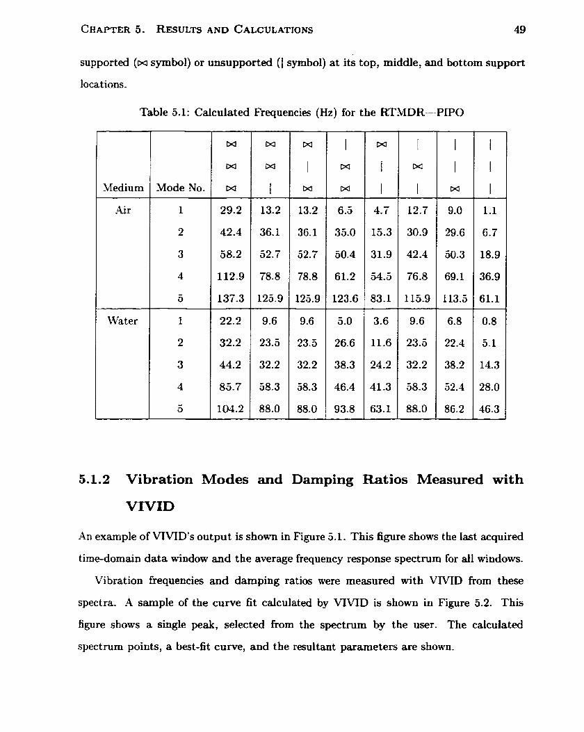
supported (w symbol) or unsupportecl ( 1 symbol) at its top, middle, and bottom support
locations.
Table 5.1: Calculated Frequencies (Hz) for the RTMDR--PIPO
Medium
Air
Water
Mode No. 1 w
5.1.2 Vibration Modes and Damping Ratios Measured with
VWID
An example of VIVID's output is s h o w in Figure 5.1. This figure shows the Iast acquired
time-domain data window and the average fkquency response spectrum for ail windows.
Vibration kequencies and darnping ratios were measured wit h VNID from t hese
spectra. A sample of the curve fit calculated by WVID is shown in Figure 5.2. This
figure shows a single peak, selected from the spectrum by the user. The calculated
spectrum points, a best-fit curve, and the resultant parameters are shown.
CHAPTER 5 . RESULTS AND CALCULATIONS 50
Vibration frequency and damping ratios for al1 RTMDR tests are shown in Table 5.2.
These values are the averages of al1 midspan amplitude spectra wit h distinguishable
peaks (Le., up to six spectra, two directions at each rnidspan). Blank entries indicate
that VIVID analysis found no distinguishable peaks.
Table 5.2: RTMDR Fre
Water a
uencies and Dam
Vibration
Frequency (Hz)
h g Ratios
Damping
Ratio (%)
5.1.3 Midspan Amplitudes for Water Tests Measured with VIVID
Midspan amplitudes were measured for al1 water tests to calculate energy dissipation due
to viscous damping. Those measurements are given in Table 5.3.
Table 5.3: RTMDR -%fids~an Ani~litudes
Shaker
Power Level
Top Midspan
Amplitude ( ~ m )
Middle Midspan
Amplitude ( ~ m )
Bottom Midspan
Amplitude (pm)
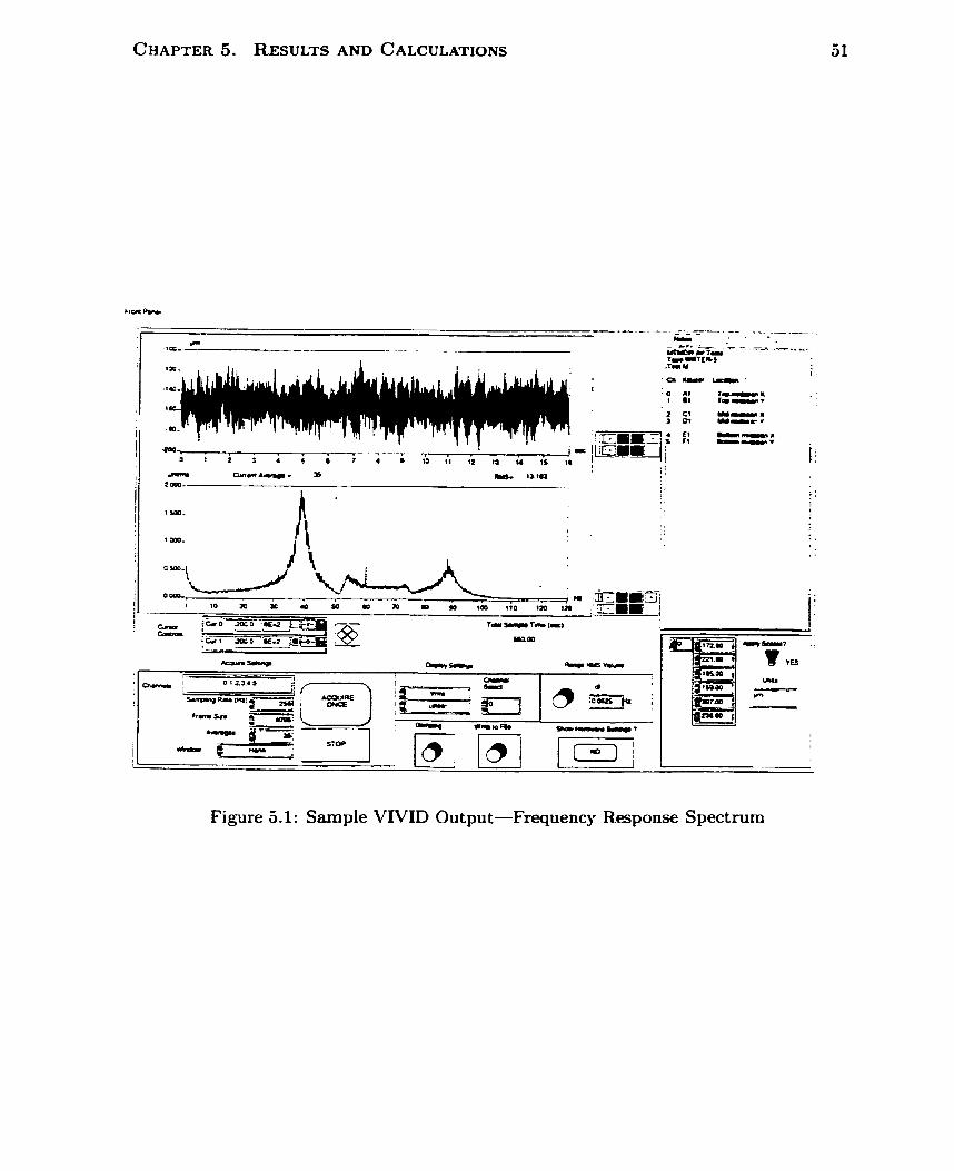
CHAPTER 5 . RESULTS AND CALCULATIONS
Figure 5.1: Sample VIVID Output-Frequency Response Spectrum
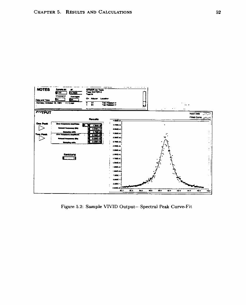
CHAPTER 5 . RESULTS AND CALCULATIONS
Figure 5.2: Sample VIWD Output-SpectraI Peak Curve-Fit
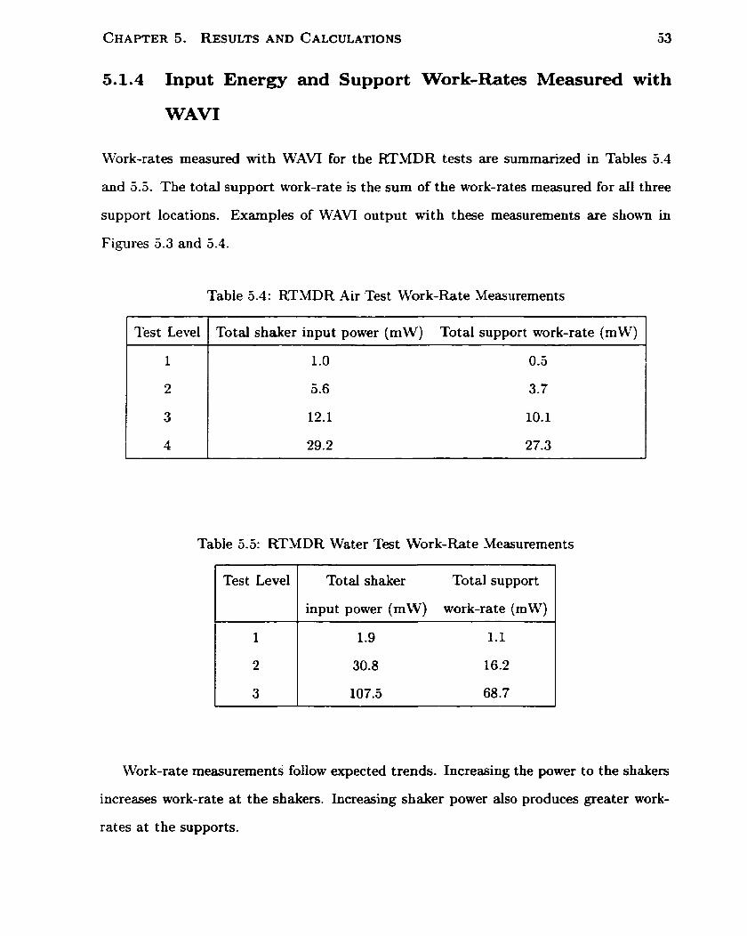
CHAPTER 5. RESULTS AND CALCULATIONS 53
5.1.4 Input Energy and Support Work-Rates Measured with
WAVI
Work-rates measured with WAVI for the RTMDR tests are summarized in Tables 5.4
and 5.5. The total support work-rate is the sum of the work-rates measured for al1 three
support locations. Examples of WAVI output with these measurements are shown in
Figures 5.3 and 5.4.
Table 5.4: RTMDR Air Test Wbrk-Rate Measurements
Test Level Total shaker input power (mW) Total support work-rate (mW) 1
Table 5.5: RTMDR Water Test Work-Rate Measurements
Work-rate measurements follow expected trends. Increasing the power to the shakers
increases work-rat e at the shakers. Increasing shaker power also produces great er work-
rates at the supports.
Test Level Total shaker Total support
input power (mW) work-rate (mW)

CHAPTER 5. RESULTS AND CALCULATIONS
Y - . . . :
Figure 5.3: SampIe W N I Output-Support Work-Rate
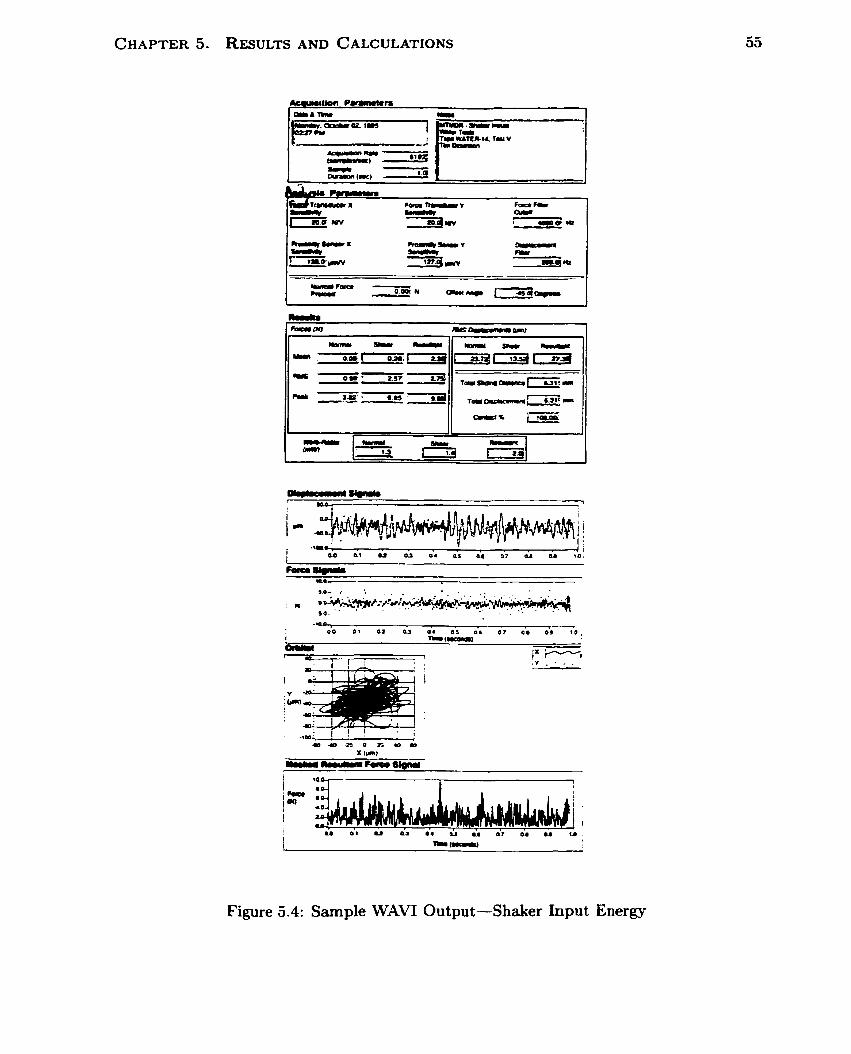
-- O * ,
Figure 5.4: Sarnple WAVI Output-Shaker Input Energy

Damping Ratio Estirnates fiom Input Work-Rates
The effective rnass expression
can be simplified by the small confinement ratio value. The confinement effect c, is
and since is small (the tube is several diameters away from the rig walls) , c, is
approxirnately 1 .O and the m a s Equation 5.1 becomes
From published water property tables [l?] and the tube properties found in Table 3.1
the tube density (phk) is 7944 kg/m3, the water density is ( ~ ~ ~ ~ r ~ ~ ~ o ~ ) is 997 kg/rn3,
the tube outer diameter (Do) is 15.9 mm, the tube inner diarneter (Di) is 13.7 mm, and
the water viscosity (v) is 0.906 x 10-~ rn2/s, from which the effective mass per unit tube
Iength is
n = 0.751 kg/m
From Equation 2.9, the effective mass of an RTMDR span is then calculated to be:
In Subsection 2.4.1 it was assurned that the amplitude of vibration is twice the RUS
value. As an example calculation, the results from Test Level 1 of the RTMDR water
test midspan amplitudes are:
60 pm x 2 = 120 pm at the top midspan
38 pm x 2 = 76 pm at the middle midspan
40 prn x 2 = 80 pm at the bottom rnidspan

CHAPTER 5. RESULTS AND CALCULATIONS
The average vibration amplitude is:
From Table 3.5 the shaker input power for Test Level 1 in water is 1.9mW. -4t a
measured frequency of 24 Hz, this corresponds to an energy input of 79.2pJ/cycle.
From earlier calculations, the effective vibrating tube mass per span is 0.458 kg. Thus:
for the three spans, the total effective tube m a s is 1.374 kg.
From Equation 2.8, the equivalent viscous damping based on dissipated input energy
is:
Sirnilar calculations produce total equivalent viscous damping values for each test
case for the RT-MDR in air and in water. These results are contained in Table 5.6.
Table 5.6: RTMDR Damping Ratio Estimates from Energy Dissipation
1 Medium Test level
Air 1
2
3
4
Water 1
2
3
Total damping ratio (%)
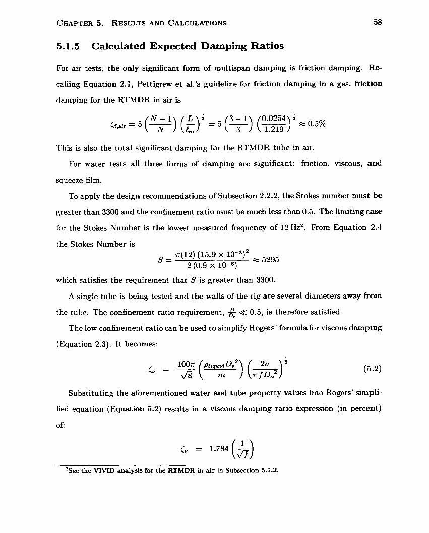
CHAPTER 5 . RESULTS AND CALCULATIONS
5.1.5 Calculated Expected Damping Ratios
For air tests, the only significant form of rnultispan darnping is friction darnping. Re-
calling Equation 2.1, Pettigrew e t a l . ' ~ guideline for fnction damping in a gas, fnction
damping for the RTMDR in air is
This is also the total significant damping for the RTMDR tube in air.
For water tests al1 three forms of damping are significant: friction, viscous, a n d
squeeze-film.
To apply the design recommendations of Subsection 2.2.2, the Stokes number must be
greater than 3300 and the confinement ratio must be much less than O.S. The Iimiting case
for the Stokes Number is the lowest measured frequency of 12 Hz2. From Equation 2.4
the Stokes Number is
which satisfis the requirement that S is greater than 3300-
A single tube is being tested and the walls of the rig are several diameters away from
the tube. The confinement ratio requirement, & « 0.5, is therefore satisfied.
The low confinement ratio can be used t o simplih Rogers' formula for viscous darnping
(Equation 2.3). It becomes:
Su bstituting the aforementioned water and tube property values into Rogers' simpli-
fied equation (Equation 5.2) results in a viscous darnping ratio expression (in percent)
of:
2See the VIVID analysis for the RTMDR in air in Subsection 5.1 -2.
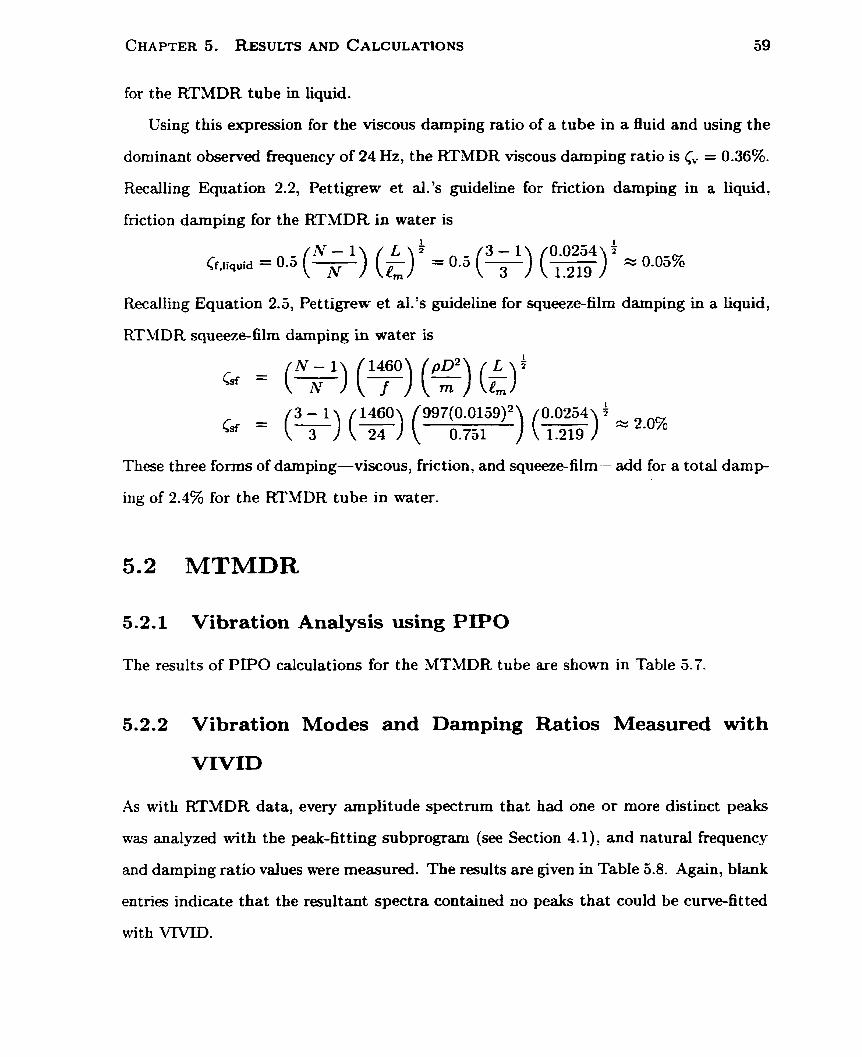
for the RTMDR tube in liquid.
Using this expression for the viscous damping ratio of a tube in a fluid and using the
dominant observed frequency of 24 Hz, the RTMDR viscous damping ratio is C, = 0.36%.
Recalling Equation 2.2, Pettigrew et al.% guideline for fiction damping in a liquid,
friction damping for the EYTMDR in water is
Recalling Equation 2.5, Pettigrew et al.% guideline for squeeze-film damping in a liquid,
RTMDR squeeze- film damping in water is
These three forms of damping-viscous, friction, and squeeze-film-add for a total d a m p
ing of 2.4% for the RTMDR tube in water.
5.2 MTMDR
5.2.1 Vibration Analysis using PIPO
The results of PIPO calculations for the MTMDR tube are shown in 'Table 5.7.
5.2.2 Vibration Modes and Damping Ratios Measured with
As with RTMDR data, every amplitude spectrum that had one or more distinct peaks
was analyzed with the peak-fitting subprogram (see Section 4.1): and natural frequency
and damping ratio values were measured. The results are given in Table 5.8. Again, blank
entries indicate that the resultant spectra contained no peaks that could be curve-fitted
with VTVID.
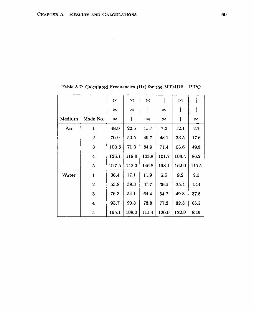
Table 3.7: Calculated Frequencies (Hz) for the MTY DR -PIPO
Air
Mode No.
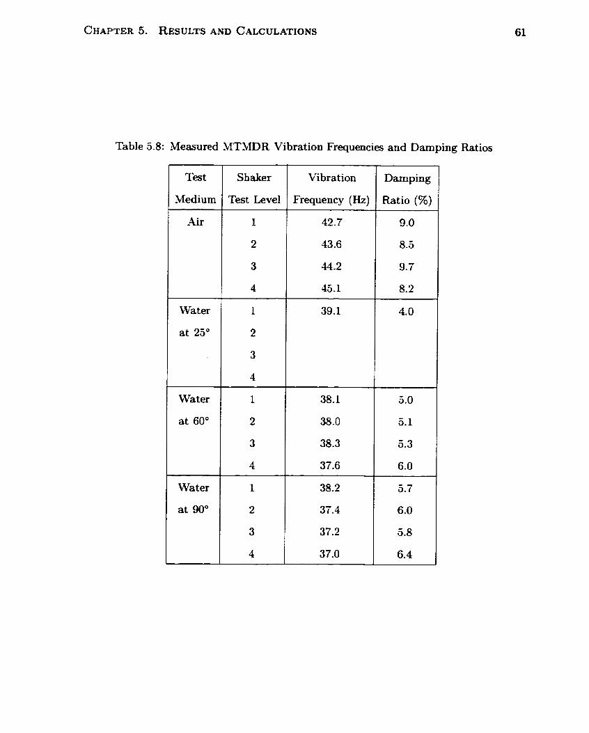
CHAPTER 5. RESULTS AND CALCULATIONS
Table 5.8: Measured MTMDR Vibration Frequencies and Damping Ratios
Test 1 Shaker 1 Vibration / Damping
Medium
-4ir
Water
at 60"
Water
at 25"
Test Level
1
Frequency (Hz) 1 Ratio (%)
42.7 1 9.0
4
1
2
Water
at 90"
45.1
39.1
4
1
2
3
8.2
4. O
37.6
38.2
37.4
37.2
6.0
5.7
6.0
5.8

CHAPTER 5. RESULTS AND CALCULATIONS 62
5.2.3 Midspan Amplitudes for Water Tests Measured with VIVID
Midspan amplitudes were measured for al1 water tests to caiculate energy dissipation due
to viscous damping. Those measurements are given in Table 3.9.
Medium 1 Shaker
( Power Level
Water
at 25°C
Water 1 1
Water
at 90°C
5.9: MTMDR M
Top Midspan
Amplitude (pm)
ispan Amplitudes
Amplitude ( p m ) 1 Amplitude (pm)
Middle Midspan
5.2.4 Input Energy and Support Work-Rates Measured with
WAVI
Bottom Midspan
Work-rates measured with WAVI are shown in Table 5.10 (air tests) and 3.11 (water
tests).
These measurements follow expected patterns. Increasing shaker power produces
increasing work-rates measured at the shakers and at the supports. As with the RTMDR,
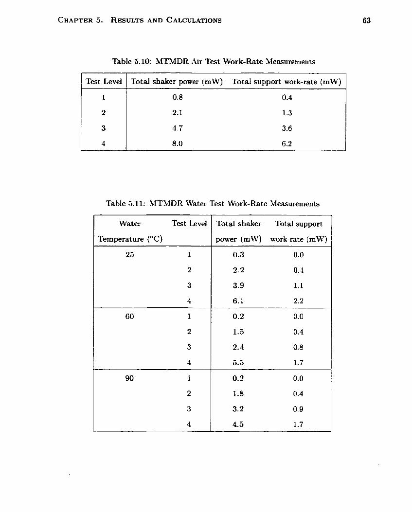
Table 5.10: MTMDR Air Test Work-Rate Measurements
1 Test Level 1 Total shaker power (mW) Total support work-rate (mW)
Table 5.11: -MTMDR Water Test Work-Rate Measurements
Wa t er Test Level
Temperature (OC)
Total shaker Total support
power (m W) work-rate (mW)

CHAPTER 5. RESULTS AND CALCULATIONS
the sum of the support work-rates in air is slightly less than the shaker work-rates.
Damping Ratio Estimates From Input Work-Rates
Damping ratios from input power dissipation are shown in Tables 5.12 and 5.13. Calcu-
lations are the same as those done in Subsection 5.1.4.
Table 5.12: Damping Ratio Estimates from Shaker Work-Rates for the MTMDR in Air
5.2.5 Calculated Expected Damping Ratios
Test
level
Using Equation 2.1 -Pet tigrew et al.'s guideline for friction damping in a gas-friction
Total damping
ratio (%)
damping for the MTMDR in air is cf,,, = 0.6%.
From Equation 2.4): the limi ting case Stokes number (i.e., lowest frequency and high-
est viscosity) is
which is greater than 3300.
Here as well, the confinement ratio & « 0.5, since only a single tube is being tested
and the walls of the rig are several diameters away from the tube.
Water density, viscosity, and tube effective mass per unit length are shown in Ta-
ble 5.14. Since the water parameters are temperature-dependent, the effective m a s is
slightly different for each test ing temperature.
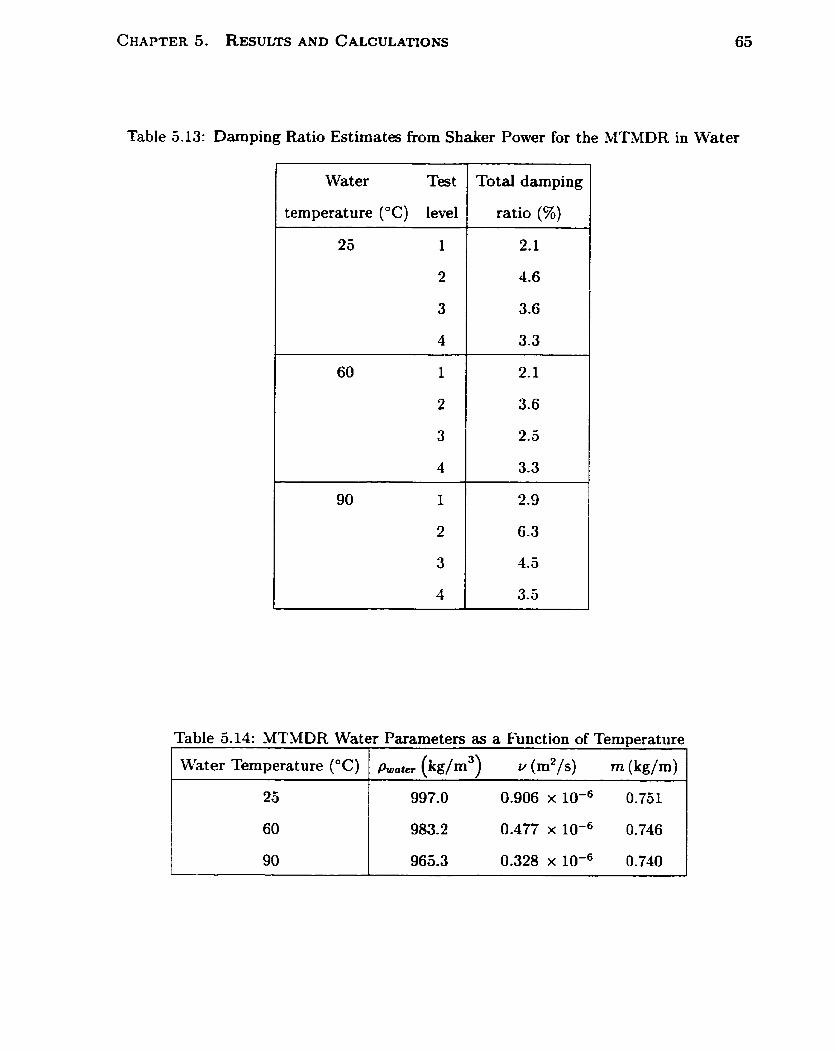
CHAPTER 5. RESULTS AND CALCULATXONS
Table 5.13: Damping Ratio Estirnates from Shaker Power for the MTMDR in Water
Water Test
temperature (OC) level
Total damping
ratio (%)
Table 5.14: MTMDR Water Parameters as a Function of Temperature
\Vater Temperature (OC)
25
p,.t., (kg/rn3) v (m2/s) m (kg/m)
997.0 0.906 x 10-~ 0.751

CHAPTER 5. RESULTS AND CALCULATIONS 66
Substituting these values into Equation 5.2 results in an expression for MTMDR v i s
cous damping ratio for each test temperature. These expressions are shown in Table 5-15.
For the dominant observed frequency of 45 Hz, the MTMDR viscous damping ratios
are :
Table 5.15: Viscous Damping Ratio Expressions for the MTMDR Tube in Water
Recalling Equation 2.2, friction damping for the MTMDR in water is C r , g = 0.1%:
and for Equation 2.5, values for MTMDR squeeze-film damping in water are
Water Temperature (OC)
25
60
90
Total damping ratios for the water tests are 1.6% for tests a t 25" C , and 1.5% for tests
at 60" C and 90" C.
Viscous Damping Ratio Equation (%)
1.781 " = 7 1.283 " = J I
"='J"' f
1
Chapter 6
Discussion
The results reported previously are discussed in this chapter in iight of the objectives of
this work.
Output fiom VIVID and WAVI are sometimes shown in figures in this section for
illustration. Examples are not given for every case, since the quantity of results horn
VIVID and WAW is too large for complete inclusion in this document.
6.1 Comparing Vibration Frequencies Measured wit h
VIVID and PIPO Results
PIPO is a validated code. Modes calculated with PIPO represent vibrating tubes with
clamped and pinned boundary conditions. Although RTMDR and MTMDR tube sup-
port conditions are not perfectly clamped and pinned, agreement between fiequencies
calculated with PIF0 and measured with VIVID are evidence that the correct vibration
modes are identified.
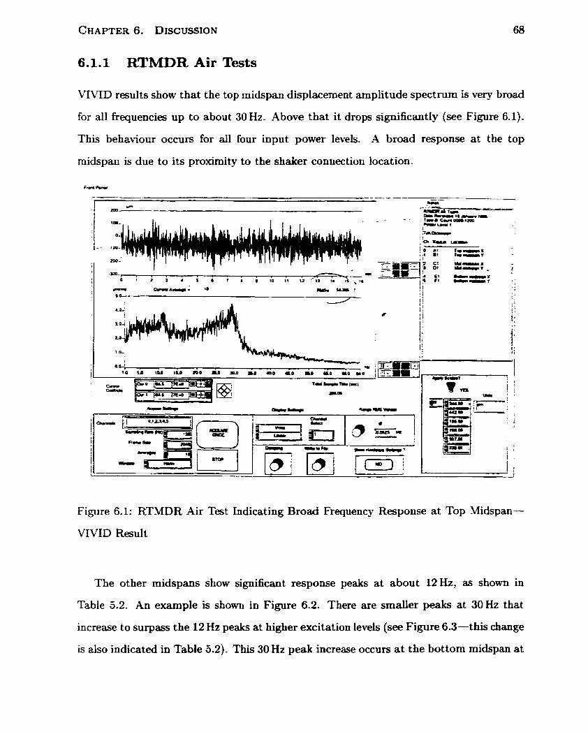
6.11 RTMDR Air Tests
VIVID results show that the top rnidspan displacement amplitude spectrurn is v e l broad
for al1 frequencies up to about 30 Hz. Above that it drops significantly (see Figure 6.1).
This behaviour occurs for al1 four input power levels. -4 broad response at the top
midspan is due to its proximity to the shaker connection location.
Figure 6.1: RTMDR Air Test Indicating Broad Frequency Response a t Top Midspan-
VIVID Result
The other midspans show significant response peaks a t about 12 Hz, as shown in
Table 5.2. An example is shown in Figure 6.2. There are smaller peaks at 30 Hz that
increase to surpass the 12 Hz peaks at higher excitation levels (see Figure 6.3-this change
is also indicated in Table 5.2). This 30 Hz peak increase occurs at the bottom midspan at

Figure 6.2: RTMDR Air Test 12 Hz Peak at Middle Midspan-VNID Result

low excitation levels and occurs a t the middle and upper midspans at higher excitation
levels.
Figure 6.3: RTYDR Air Test 30Hz Peak Growing with Increased Excitation at Middle
Midspan-VIVID Result
PIPO predicts a fundamental natural frequency of 13.2 Hz (Table 5.1) for the case
where only the top and middle supports are effective. Tbese values correspond with the
12 Hz response peak seen at low power levels (the bottorn support was the only one where
the tube was properly centered). At low input forces the tube did not contact the bottom
support. The support was ineffective.
At higher excitation levels, as indicated . above, the dominant amplitude spectrum
peak changed to 30Hz. The PIPO results of Table 5.1 indicate that the fundamental
mode of the dl-supportseffective case is very close to this (29.2 Hz). At these levels the

tube is contacting the bottom support more often and al1 supports are effective.
6.1.2 RTMDR Water Tests
As found in the air tests, the top midspan displacement amplitude spectrum is very broad
up to about 23 Hz for al1 levels (see Figure 6.4).
O-- - b L Y . C I 8 . l r-O Cri-
;'-
. O Ai T i r 'I m* 70- v
El - x . s CI rm-t
Figure 6.4: RTMDR Water Test with Broad Frequency Response at Top Midspan-
WVID Result
The middle and bottom midspan displacement frequency spectra each show a peak
at approximately 24 Hz for al1 power levels (see Figure 6.5 and Table 5.2).
Table 5.1 indicates that PIPO predicts a fundamental frequency of 22.2Hz for the
dl-supports-effective case of the RTMDR in water. This is a reasonable match with the
measured frequency since al1 supports were preloaded.

Figure 6.5: RTMDR Water Test 24 Hz Peak at Middle Midspan-VIVID Result

6.1.3 MTMDR Air Tests
Top and middle midspan measurements produced the most distinct vibration peaks. The
Iargest occurs a t approximately 43 to 45 Hz. The averages are reported in Table 5.8, and
an example is shown in Figure 6.6.
Figure 6.6: MTMDR Air Test 44 Hz Peak-WVID Result
From Table 5.7, PIPO predicts a fundamental natural frequency of 48 Hz for three
effective supports. This is close to the measured value.
6.1.4 MTMDR water tests
The natural frequencies measured in MTMDR water tests using VTVID are shown in
Table 5.8. They are d l approximately 38 Hz. PIPO predicts a natural frequency of

36.4 Hz for an .MTMDR tube in water with d l supports effective.
Damping Ratios Measured with VIVID from Fre-
quency Responses
6.2.1 RTMDR Air Tests
Damping ratios measured with MVID mried significantly, fmm 2% to 8%. Averages,
again, are in Table 5.2. An example is shown in Figure 6.7.
Figure 6.7: Sample RTMDR Air Darnping Ratio-VIVID Result
Previous experimentation by Pet tigrew et al. [5] indicates t bat heat exchanger tube
damping ratios in air are typically near 1%. One possible reason for the large damping
ratios measured by VIVID in these tests is that even the two-peak analysis is a sim-

plification of the non-linear tube dynamics. The non-linearities of a tube contacting
its supports at different points, or of different tube material properties, may not be so
discrete. -4 close "cluster" of spectral peaks could emerge that rnay show up as one or
more broadened peaks. Such peaks rnay still center on the correct fiquency. The peak
broadness implies an exaggerated damping ratio in the same way that fit ting two peaks
with a single curve would.
6.2.2 RTMDR Water Tests
-4s in air tests, damping ratios rneasured with V M D in water tests were large-between
8% and 10% as pouer levels increased (see Figure 6.8 and Table 5.2).
c-4- . . . . . . . . . .. J ; 1- iu 1~ ara =O a n 140 MO w n.o no a o .
Figure 6.8: Sample RTMDR Water Damping Ratio-VWID Result

6.2.3 MTMDR Air Tests
Damping ratios rneasured with V N I D fkom the top and middle midspan responses varied
between 8% and 1 l%, with averages shown in Table 5.8. These are also larger than the 1%
range predicted by Pettigrew et al. The reasons are the same-probably non-linearities
of the tube/support interaction.
6.2.4 MTMDR Water Tests
Damping ratios for MTMDR water tests are also given in Table 5.8. Average rarige from
4% to more than 6%.
These results are unusual. Damping ratios measured increased slightly with temper-
ature. It was expected that damping would decrease with increased water temperature
as water viscosity decreases.
6.3 Darnping Ratio Cornparisons
Figures 6.9 to 6.14 contain graphs comparing damping ratios calculated or estirnated
from each of three methods: Pet tigrew et a1.k equations, cuwe-fi t ting frequency response
peaks with VIVID, and the dissipation rate of the input energies rneasured by WAVI.
In al1 cases, the graphs indicate that the damping values measured with the two
test methods are always greater than Pettigrew et a1.k guidelines. This is expected,
since the guidelines are a lower bound of many experirnental data and meant to make a
conservative (i.e., worst-case) estimate of darnping.
At almost every data point, damping measured by spectral peak cuwe-fits is greater
than that estirnated from input energy. This is probably due to the aforementioned dif-
ficulty in estimating damping from spectral curve-fits: non-lineaxities contribute to peak
broadening resulting in incorrect ly large damping estimates. Estimating damping from
the dissipated input energy avoids this difficulty, and produces lower damping estimates

that are closer to the guideline values.
There does not appear to be any significant effect of excitation level on damping in
any of the graphs (Figures 6.10. 6.12, 6.13: and 6.14). This agrees with the previous
experimental data bounded by Pettigrew et d ' s guidelines.
There does not appear to be any significant effect of temperature on damping in
the water test results. While this agrees with Pettigrew et a1.k guidelines: it is not
immediately clear why there should be no temperature effect. The viscosity of water
decreases by a factor of nearly three between 25" C and 90" C. It might be q e c t e d
that this changing viscosity would have a significant impact on viscous and squeeze-film
damping. One possible explanation for the lack of temperature effect is that a t higher
temperatures the fluid viscosity will be lower, but the fluid film between the tube and
support may be thinner. The decrease in damping due to the lower viscosity of the
squeezed fluid may be offset by an increase in damping due to the greater constriction
of the tube/support gap allowing displacernent of the squeezed fluid. The absence of
temperature effect is still under investigation, however.
It is important to note that the da ta reported in the graphs is highly statistical
in nature. That is, there are a number of factors (e-g., tube/support preloading o r
clearances, bent tubes) that c m change with every test. These factors can explain the
small variations in damping seen between different tests. These factors also imply that
these tests form one or two statistical "points" in the group of test data from which
Pettigrew et al.'s guidelines were made. The real significance of this work is that these
data points were made with a new and improved damping measurement method: the
work-rate method.

-
UWûR Air Test
- - Design Guide(ine Lower Bound + C m i i t Spectral Peak (VNID) -- Dissipaled hpit En= (WAVI)
Figure 6.9: RTMDR Air Test Damping Ratios

RTMûR Weter Test
12 - - - Design Guideliri4 Lcmer Bainci +- C h r e m Spectral Peak (VNlD) -- - Dissimed Inpuî Enegy (WAVI)
O
O 20 40 60 80 1 0 0 l a )
Sh8L.r input Powor (mW)
Figure 6.10: RT-MDR Water Test Damping Ratios

6 - -- - - Design Guideiine Laww Bound + Cum-fil Spectral Peak (VIVID)
5 - -- : Dissipatedlnprt Energy (WAVi) .-
1 -
0 - P
O 1 2 3 4 5 6 i 8 - Shmlur ln@ Powar (mW)
Figure 6.11: MTMDR Air Test Damping Ratios

8 -
-- - Design Gutddine iower Band -f- bw+fil SpsEtral Peak (VNID) 7 - -- - Dissipated hprt Enagy (WAVI)
0 - O 1 2 3 4 5 6 7
S b b r Input Powar (mW)
Figure 6.12: MTMDR ?Vater at 25" Test Damping Ratios

8 - - . - Design Guiddine Loiiuer Barnd +- C w f t t Spectral Peak (VNID) --
7 - - Rssipad Input Encrgy (WAVI)
Figure 6.13: MTMDR Water at 60" Test Damping Ratios
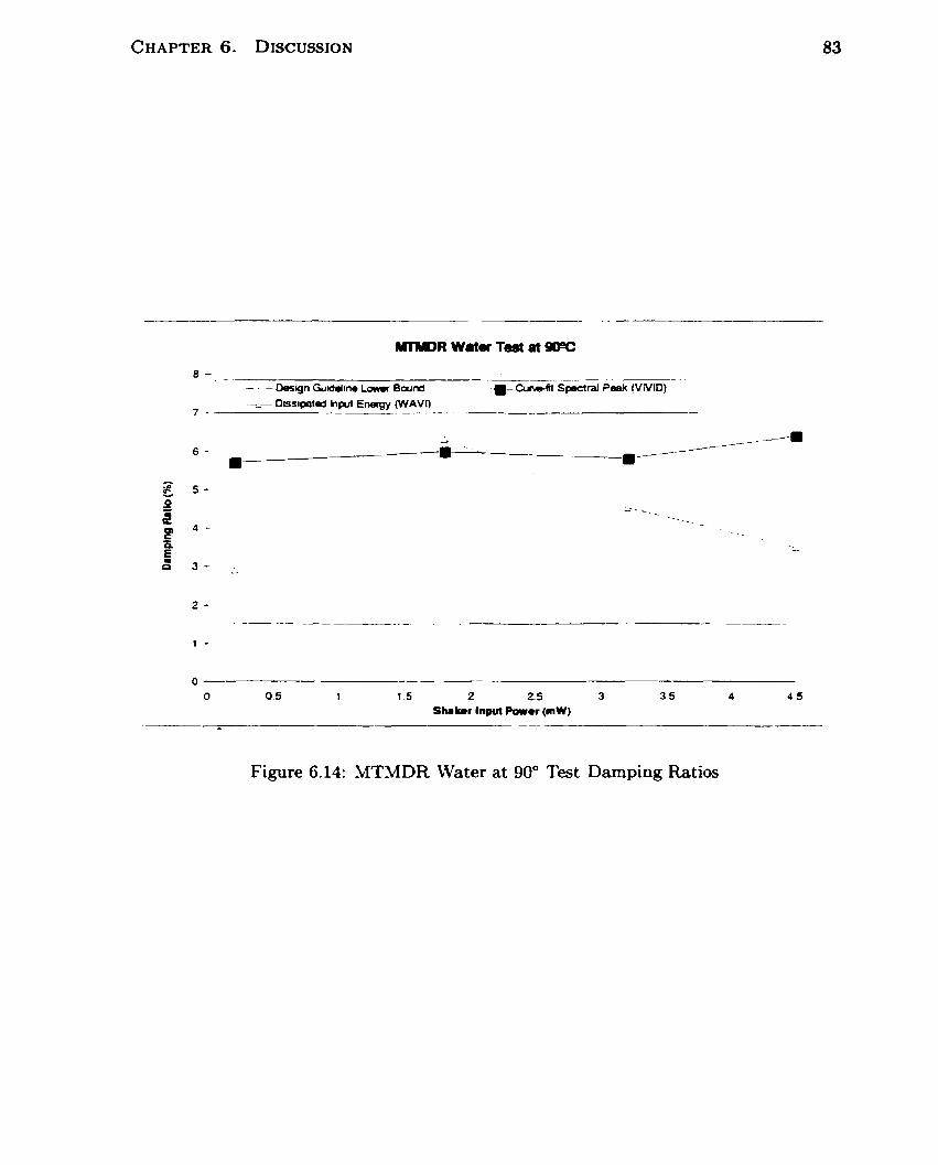
8 - - . - Design Guiddine Laul.r Bwnd - Cuirblil Spsctral Pmk [VIVID)
Figure 6.14: MTMDR Water at 90" Test Damping Ratios
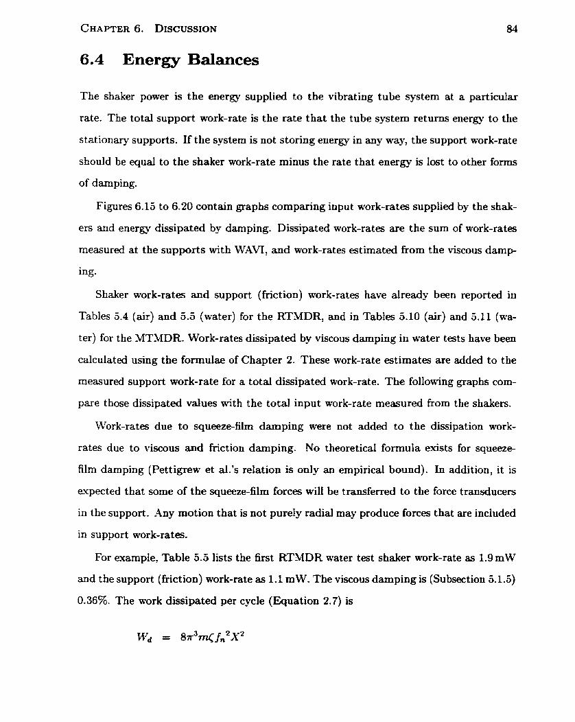
6.4 Energy Balances
The shaker power is the energy supplied to the vibrating tube system at a particular
rate. The total support work-rate is the rate that the tube system retums energy to the
stationary supports. If the system is not storing energy in any way, the support work-rate
should be equal to the shaker work-rate minus the rate that energy is lost to other forms
of damping.
Figures 6-15 to 6.20 contain graphs comparing input work-rates supplied by the shak-
ers and energy dissipated by damping. Dissipated work-rates are the sum of work-rates
measured at the supports with WAVI, and work-rates estimated from the viscous darnp-
ing.
Shaker work-rates and support (fnction) work-rates have already been reported in
Tables 5.4 (air) and 5.5 (water) for the RTMDR, and in Tables 5.10 (air) and 5.11 (wa-
ter) for the YTMDR. Work-rates dissipated by viscous damping in water tests have been
calculated using the forrnulae of Chapter 2. These work-rate estimates are added to the
measured support work-rate for a total dissipated work-rate. The following graphs com-
pare those dissipated values with the total input work-rate measured from the shakers.
Nrork-rates due to squeeze-film damping were not added to the dissipation work-
rates due to viscous and fnction damping. No theoretical formula exists for squeeze-
film damping (Pettigrew et a1.k relation is only an ernpirical bound). Ln addition, it is
expected that some of the squeeze-film forces will be transferred to the force transducers
in the support. Any motion that is not purely radial may produce forces that are included
in support work-rates.
For example, Table 3.5 lists the first RTMDR water test shaker work-rate as 1.9mW
and the support (friction) work-rate as 1.1 mW. The viscous damping is (Subsection 5.1.5)
0.36%. The work dissipated per cycle (Equation 2.7) is

which, at a frequency of 24 Hz, corresponds to 0.1 mW. Adding this to the support work-
rate results in a total dissipated work-rate of 1.2 mW. Similar calculations are made for
al1 other water tests for both rigs.
The sum of the support work-rates is very close to the shaker power for air tests.
This is expected for air tests since the only significant contribution to the darnping is
friction. It is also expected that the input-output diReremes are greater for the water
tests. Viscous and squeeze-film darnping would add to the total darnping for a tube
vibrating in water.
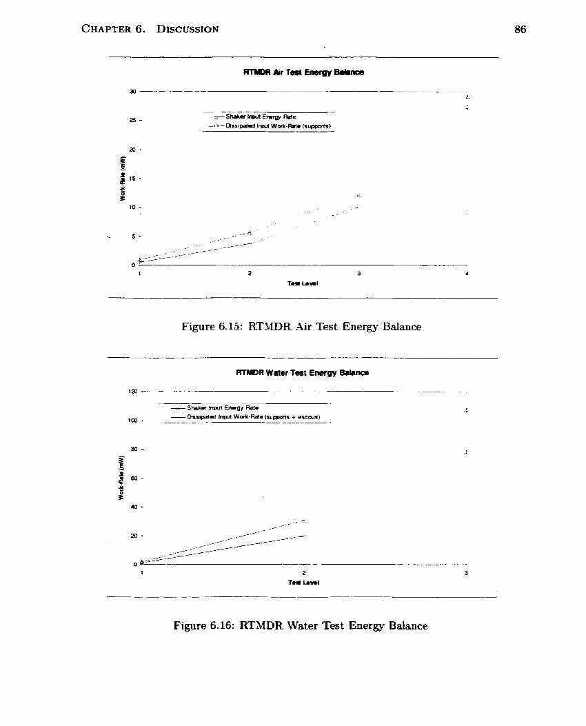
Figure 6.15: RTMDR Air Test Energy Bdance
Figure 6.16: RTMDR Water Test Energy Bdance
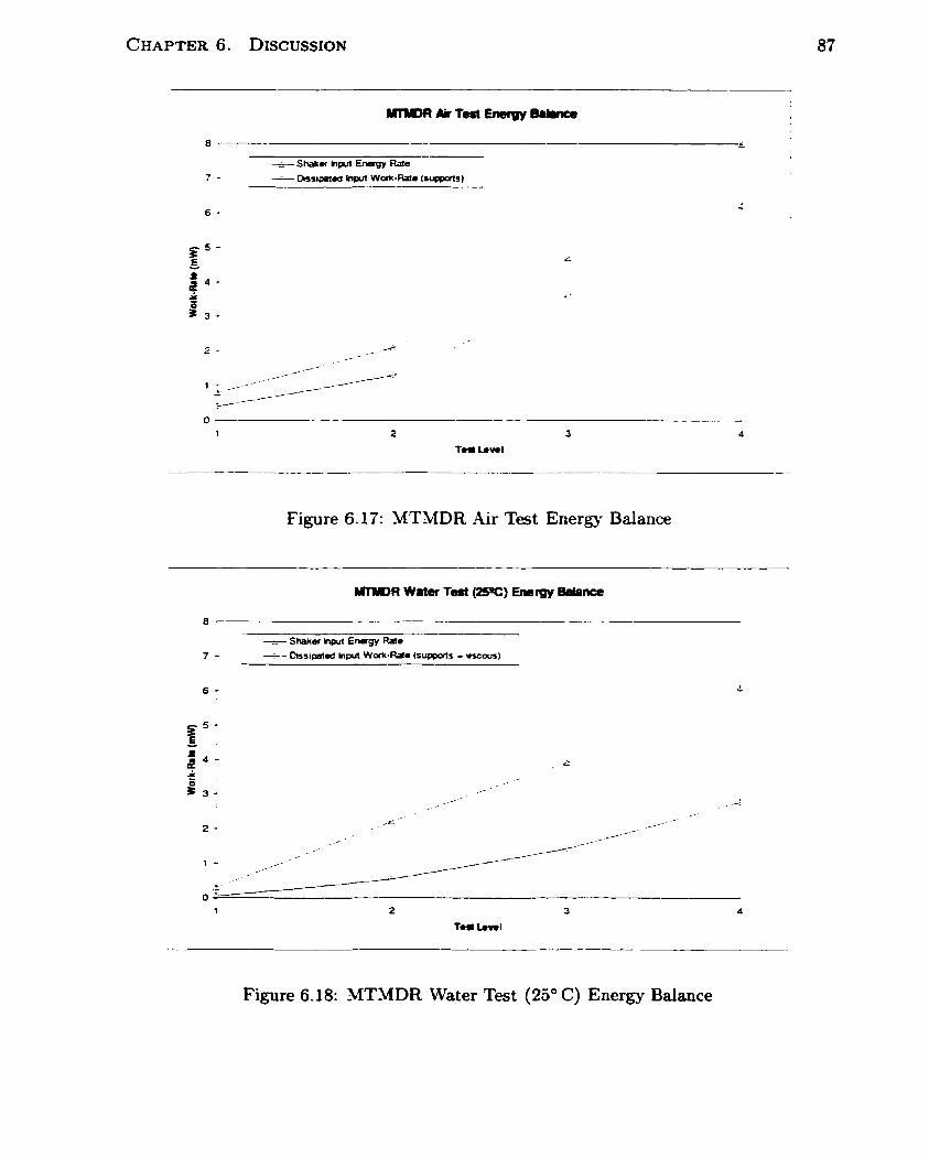
8 -.- -=-- Shalra hm E n w M e
7 - - - Dnsiptid hpuî Wak-m~ (S-1
Figure 6.17: MTMDR .&r Test Energ). Balance
Figure 6.18: MTMDR Water Test (26" C) Energy Balance
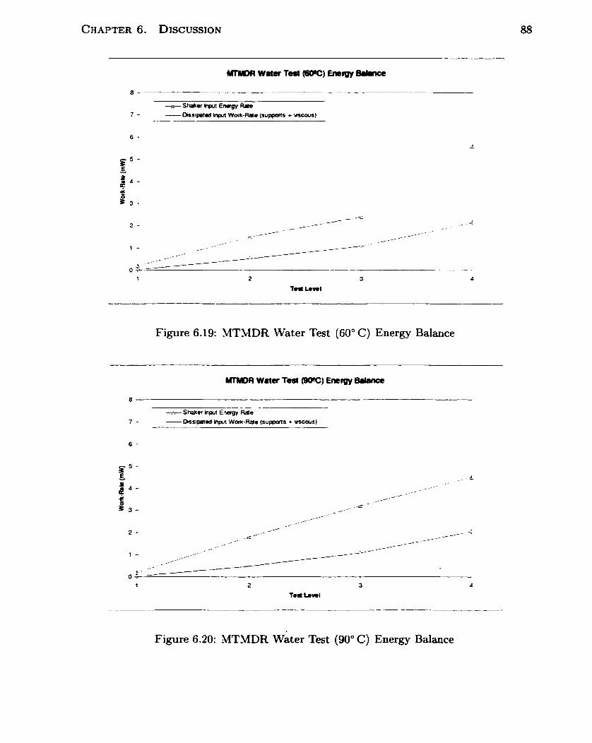
Figure 6.19: MTMDR Water Test (60" C) Energy Balance
Figure 6.20: MTMDR ~ a t e r Test (90" C) Energy Balance

Chapter 7
Conclusions
This thesis describes work done to understand damping in multispan heat exchanger
tubes.
-4 test facility was developed to measure damping of multispan heat exchanger tubes
in air and in water a t different temperatures up to 90°C. This rig is now used for further
damping studies.
A computer program narned VIVID was developed and used to measure hequency
response and tube vibration amplitudes. It can also calculate system parameters such as
natural hequency and damping fiorn curve fits of the frequency response. This software
has a simple user interface, d o w s several channels of data to be analyzed simultaneously,
and contains advanced numencal routines to allow curve-fi tting of two adjacent spectral
peaks. VNID is now used for other applications.
A computer program named WAVI was developed and used t o calculate shaker exci-
tation work-rates dissipated at rig supports. WAVI is a development of a program used
to measure work-rates in fretting-wear testing. Changes were made to improve the user
interface, and to include measurements of shaker work-rates. WAVI was essential to this
work, since an important objective was to develop a method of estimating damping using
work-rates.

As expected, damping values estirnated fIom the rate of dissipated input energy are
slightly greater than the lower lirnit values of Pettigrew et al.k guidelines. They are
less than values estimated from curve-fit ting response spectra. This was expected, since
the energy method avoids some of the limitations of the spectral peak method. This
energy method appears to be a better method of measuring damping for systems with
non-linearities and multi-peak ftequency responses, such as heat exchanger tubes.
For the air tests--where fî-iction damping at the support is the only significant d a m p
ing occurring-the support work-rate is only slightly las than the shaker work-rate?
indicating a reasonable energy balance. For water tests, the difference between the sup-
port work-rate and shaker work-rate is greater, as expected, due to the additional viscous
damping. When the viscous work-rate is added there is still a difference between dissi-
pated work-rate and shaker input work-rate: this may be due to the inability to accurately
measure or calculate the squeezefilm energy dissipation. This is the first knoun time
that energy balance and the dissipated energy approach is used to characterize d a m p
ing of heat exchanger tubes. As mentioned earlier, subsequent work has confirmeci the
validity of the energy approach.
Damping values did not change significantly wit h temperature or excitation level.
Both of these results agree with past experimental data bounded by Pettigrew et al.'s
guidelines, although further work needs to be done to determine why no temperature
effect exists.
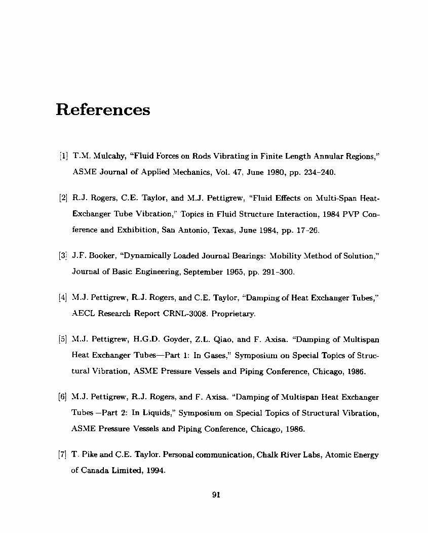
References
[l] T.M. Mulcahy, "Fluid Forces on Rods Vibrating in Finite Length Annular Regions,"
ASME Joumal of Applied bkhanics, Vol. 47. June 1980, pp. 234-240.
[2] R. J. Rogers, C.E. Taylor, and M.J. Pettigrew, "Fluid Effects on Multi-Span Heat-
Exchanger Tube Vibration," Topics in Fluid Structure Interaction, 1984 PVP Con-
ference and Exhibition, San Antonio, Texas, June 1984, pp. 17-26.
[3] J.F. Booker, 'LDynarnically Loaded Journal Bearings: Mobility Wethod of Solution,"
Journal of Basic Engineering, September 1965, pp. 291-300.
[4] M. J. Pettigrew, R. J . Rogers, and C.E. Taylor, "Damping of Heat Exchanger Tubes,"
XECL Research Report CRNL-3008. Proprietary.
[5] M.J. Pettigrew, H.G.D. Goyder, Z.L. Qiao, and F. .&sa. "Damping of Wultispan
Heat Exchanger Tubes-Part 1: In Gases," Symposium on Special Topics of Struc-
tural Vibration, ASME Pressure Vessels and Piping Conference, Chicago, 1986.
[6] M.J. Pettigrew, R.J. Rogers, and F. Axisa. "Damping of Multispan Heat Exchanger
Tubes-Part 2: In Liquids," Symposium on Special Topics of Structural Vibration,
ASME Pressure Vessels and Piping Conference, Chicago, 1986.
[7] T. Pike and C.E. Taylor. Personal communication, Chalk River Labs, Atomic Energy
of Canada Limited, 1994.
[8] S.S. Chen, M. W. Wambsganss, and J.A. Jendnejczyk. "Added Hass and Damping of
a Vibrating Rod in Confined Viscous Fluids," ASME Journal of Applied Mechanics,
Vol. 43, pp. 325-329, 1976.
[9] J. Mastorakos. "A Numerical Technique for Deducing the Dynamic Parameters from
Amplitude spectnun Functions," Technical Memorandum SP-VIBR-73, Chalk River
Nuclear Laboratories, May 1984.
[IO] D. W. Yarquardt . "An Algonthm for Least-Squares Estimation of Nonlinear Param-
eters," Journal Society Industrial Applied Mathematics, Vol. 11, No. 2, June 1963,
pp. 431 -441.
[II] W. Press, B. Flannery, S. Teukolsky, and W. Vetterling. "Numerical Recipies," Cam-
bridge University Press, 1989.
[12] N.J. Fisher, A.B. Chow, and M.K. Weckwerth. "Experimental Fretting-Wear Studies
of S team Generator Materials," ASME PVP-Vo1.273, Flow-Induced Vibration, pp.
241-255, 1994.
[13] W.T. Thomson, 'Theory of Vibration with Applications, 3rd ed.:" Prentice Hall,
1988? pp. 61-71, 74-75.
[14] C.E. Taylor, M.J. Pettigrew, T.J. Dickinson, I.G. Curie, P. Vidalou, "Vibration
Damping in Multispan Heat Exchanger Tubes," ASME Journal of Pressure Vesse1
Technology, 1998, 120 (3), pp. 283-289.
[l5] M.J. Pettigrew, C.E. Taylor, N. J. Fisher, M. Yetisir, B.A. W. Smith, "Flow-Induced
Vibration: Receat Findings and Open Questions:' Nuclear Engineering and Design,
1998, 185, pp. 249-276.

[16] M. Yetisir, E. McKerrow, M. J. Pet tigrew, "Fret ting-wear Damage of Heat Exchanger
Tubes: A Proposed Damage Criterion Based on Tube Vibration Response," ASME
Journal of Pressure Vesse1 Technology, 1998, 120 (3)? pp. 297-305.
[l?] I.H. Shames, "Mechanics of Fluids, 2nd ed.," McGraw-Hill, 1982, p. 8-36.

Appendix A
LabVIE W and Data Acquisition
Paramet ers
This appendix briefiy describes LabVIEW and the data acquisition hardware used for
measurements.
VTU is using software developed with LabVIEW because of the programos versatili ty,
portability, and customizable graphical user interfaces. It was logical to use LabVIEW
to create specialized tools for the measurements and calculations this work required.
A . l LabVIEW
LabVTEW for Windows Version 3.0. l1 runs under Microsoft Windows 3.1 in 386 enhanced
mode. It requires a math CO-processor, and a minimum 80386-based PC.
LabVlEW requires 2.2 M B of RAM and allocates 4 -MB of system memory by default,
in addition to memory requirements for Windows and any installed drivers. Experience
indicated that vibration frequency analysis generdly required more memory, particularly
for long averaging penods with many input channels. Analysis for this work was done on
'This was the curent version of LabVIEW at the time of this work.
94
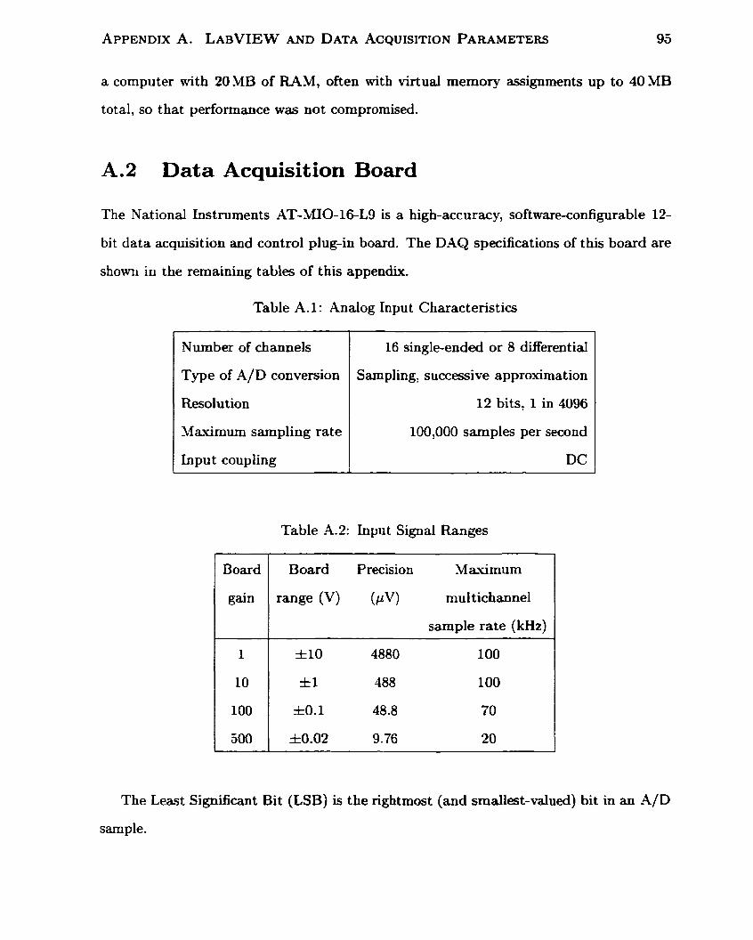
a cornputer with 20 MB of RAM, often with virtual memory assignments up to 40 MB
total, so that performance was not compromised.
A.2 Data Acquisition Board
The National Instruments i\S-MO-16-L9 is a high-accuracy, software-configurable 12-
bit data acquisition and control plug-in board. The DAQ specifications of this board are
shown in the remaining tables of this appendix.
Table A. 1 : Anaiog Input Characteristics
Nurnber of channels
Type of A/D conversion
Resolution
Maximum sarnpling rate
Input coupling
16 single-ended or 8 differential
Sampling, successive approximation
12 bits, I in 4096
100?000 samples per second
DC
Table -4.2: Input Signal Ranges
Board
gain
The Least Significant Bit (LSB) is the rightmost (and smallest-valued) bit in an A/D
sample.
Board Precision Maximum
range (V) (/IV) mu1 tichannel
1
10
100
a00
sample rate (kHz) -
3110 4880 100
+l 488 100
&O. 1 48.8 70
=t0.02 9.76 20

APPENDIX A. LABVIEW AND DATA ACQUISITION PARAMETERS
Table A.3: Transfer Characteristics
Table A.4: Amplifier Characteristics
Relative accuracy
Gain error (relative to calibration ref.)
f 0.9 LSB typical, kl.5 LSB max.
0.0244% of reading max.
Table A.5: Amplifier Common-Mode Rejec tion Ratio
Input impedance
1 Board gain 1 CMRR, DC to lOOHz (dB) 1
1 GR in paralle1 with 50 pF

The Common-Mode Rejection Ratio (CMRR) is a mesure (in dB) of an instrument's
ability to reject interference from a cornmon-mode signal.
Table -4.6: Dynamic Characteristics
Table A.7: Dynamic System Noise
Bandwidth (small signal, -3 dB)
Slew rate
1 Board gain 1 I l 0 V range
650 kHz at gain = 1
5.0 V/ps
I 5 10
100
500
0.10 LSB RUS
0.15 LSB RUS
0.30 LSB R\lS

Appendix B
VIVID
This appendix descnbes how VTU previously measured natural frequencies and damp
ing ratios from time-domain data. It also describes how the same information can be
determined using VTVID.
B. 1 Previous Procedure
The method previously used to measure twepeak damping ratios in VTU was compli-
cated. The procedure is outlined below:
1. Acquire the data and perform a spectral analysis with WAVEPAK (spectral analysis
software on a dedicated portable cornputer).
2. Estimate the six paxameters from a graph of the frequency spectnim.
3. Save the spectrum data as a special text file.
4. Edit the text file so that only the frequency and amplitude data pairs for the
spectrum remain. The text file contains other data such as parameter inputs and
time-domain input.
5 . Create a text file with estirnates of the six parameters fiom Step 2.

APPENDIX B. VIVID 99
6. Run the VTU program ~ P E A K . Supply the spectrum data file name, the frequency
range for the curve fit, and the parameter estimate file name. N PEAK iterates
and displays its final solution for parameters. If a solution is not reached (Le.,
divergence) make new parameter estimates and repeat Steps 5 and 6.
This method required transferring data between a t least three prograrns (WAVEPAK,
a tevt editor, and ~ P E A K ) . A user may have to graph the data to get an idea of suitable
initial guesses before ruming ~ P E A K . In addition, only two data channels can be acquired
by WAVEPAK at once. Repeated acquisitions and analyses are necessary if the experiment
recorded more than two channels of data.
B.2 New Procedure
The procedure developed to calculate damping ratios for this work is simpler. The
procedure is a subroutine of a larger LabVIEW analysis program (VIVID).
1. Acquire the data and perform a spectral analysis w-ith VIVID.
2. Select a channel. LabVIEW shows a new screen with a plot of the selected spectra.
3. Select one- or two-peak fitting.
4. Move graph cursors to delimit a spectral peak.
5. A dialog box appears in the top left corner of the screeu and prompts the user to
supply initial guesses.
6. Program iterates and displays its final solutions for the parameters. It also overlays
the best-fit plot over the spectral data points. The user can print this display.
Finally, control reverts back to the analysis VI. The user can then do damping
ratio cuwe fits of the other channels or acquire new data.

APPENDIX B. VIVID 100
The method is both simpler and more versatile. The user does not have to switch
between platforms and the VIS guide one through the steps with prompts and messages.
The number of data channels that can be analyzed simultaneously is greater than was
possible with WAVEPAK. The analyses done for this work were accomplished using a
data acquisition board with 16 analog input channels and a maximum total acquisition
rate of 100 kHz (e-g., 10 channels at 10 kHz each, maximum).
The structure of the damping ratio subroutine is shown below. -4 description of its
function follo~s.
Figure B. 1: Damping ratio substmcture hierarchy of VNID
When a user presses the appropriate Damping front panel button! the spectrum for the
currently-selected channel is passed to subVI DAMP. This subVI sends the information
to its own subVIs to do the iterative curve fit and retum the damping ratio parameter.
When called, a subVI named DAMP displays its front panel with three fields:
1. Input has a control for the user to select one or two peaks, a control to set the
maximum number of iterations to calculate, and buttons that will perform the
APPENDIX B. VIVID
curve fit or return to the VTVlD toplevel VI.
2. Notes displays the date and time, the channel number analyzed, sample duration
and number of averages, and analysis frequency resolution. There is also a box
where the user can enter additional information if desired.
3. Output has displays that indicate the parameters calculated after each iteration
and the current iteration number. It also has a graph that shows a plot of the
acquired hequency spectrum data points. When the iteration is done, it overlays
this information with a line plot of the calculated fit.
After the user sets the controls in Input and presses the button to perform the fit,
the following procedure executes in D AMP:
The date and time, the cbannel number, and sample data that were passed to
DAMP are displayed. The spectral data is re-plotted.
The program is paused. This allows the user to position cursors to delimit the
spectral peak (or peaks) they wish to fit.
When the Fit button is pressed, SELECT INRANGE is called to remove the part of
the spectrum the user delimited. DAMP SCALE scales that selection into a range
from O to The iterative method works more reliably when the values are scaled
wi t hin t his range. Scaled amplitudes and the corresponding hequency values are
passed to subV1 LOOPI .
SubVI GUESSES is called and the user is prompted for initial parameter values. The
user prompt appears in a small window in the upper left-hand corner of the screen
so that the user can still see the spectral plot data underneath. If there is only
one peak to be fit then there are three required inputs. If there are two peaks then
six parameters are required. Note that the default values for the zero-fiequency
amplitude and darnping ratio (0.00001 and 0.001, respectively) are nearly always
APPENDIX B. VIVID 102
adequate for the curve-fitting iteration. Users should attempt to make an accurate
guess at the peak natural frequency, however. The equations involved make the
Marquardt met hod's convergence very sensitive to t his parameter. These guesses
are returned to LOOPI.
5 . The number of iteration parameters and convergence criteria are passed to L o o ~ 2 .
6. L O O P ~ performs the calculations necessary for the Marquardt iteration met hod.
7. L O O P ~ executes in a While Loop. It stops when its convergence criteria are met
(i-e., it finds a solution) or when the iteration number exceeds the iteration limit set
by the user. The calculated parameters are scaled back to their correct values by a
cal1 to DAMP SCALE BACK and displayed on the front panel after each iteration.
8. After the Whzle Loop finishes, DAMP calculates a plot for the frequency range that
the user selected using the final values of the parameters it has calculated. This
plot is then superimposed on the spectral data.
9. The user may then repeat the process (Mth new initial guesses, for instance, if the
method did not converge) or stop the damping ratio subroutine and return to the
VIVID program.
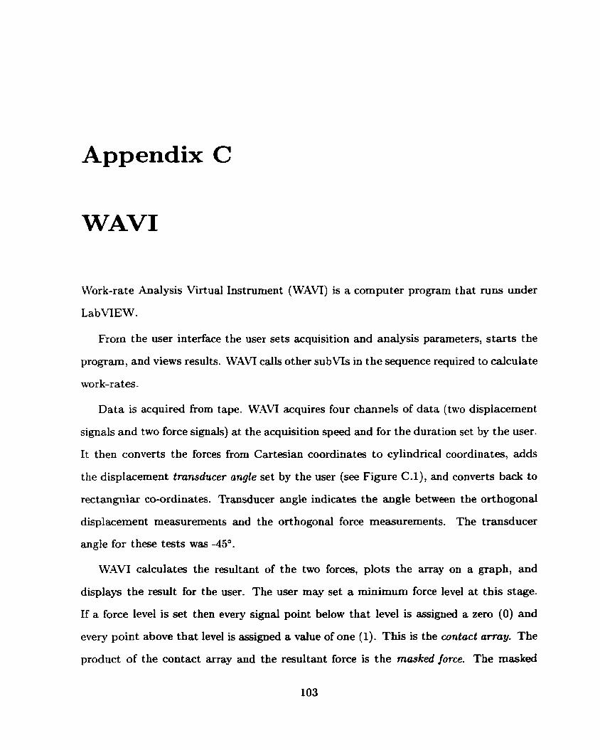
Appendix C
WAVI
Work-rate Analysis Virtual Instrument (WAVI) is a cornputer program that runs under
LabVIEW.
From the user interface the user sets acquisition and analysis parameters, starts the
program, and views results. WAVI calls other subVIs in the sequence required to calculate
work-rates.
Data is acquired from tape. WAVI acquires four channels of data (two displacement.
signals and two force signals) at the acquisition speed and for the duration set by the user.
It then converts the forces from Cartesian coordinates to cylindrical coordinates, adds
the displacement transducer angle set by the user (see Figure CJ), and converts back to
rectangular coordinates. Transducer angle indicates the angle between the orthogonal
displacement measurements and the orthogonal force measurernents. The transducer
angle for these tests was -45".
W.WI calculates the resultant of the two forces, plots the array on a graph, and
displays the result for the user. The user may set a minimum force level at this stage.
If a force level is set then every signal point below that level is assigned a zero (0) and
every point above that level is assigned a value of one f 1). This is the contact array. The
product of the contact array and the resultant force is the mwked force. The masked

APPENDUC C. WAVI
1.2,3,4 - Forces A B - Disp.
Figure C.1: Force and Displacement Transducer tayout
force is displayed for the user as well. -411 elements in the contact array are summed and
the result is divided by the size of the array and multiplied by 100%. This is the time the
tube spends in contact with the support as a percentage of t h e total sample duration.
WAVI then resotves the impact forces into normal and shear components a t the point
of contact and calculates force statistics (mean, maximum and RMS). It then takes the
displacement and contact arrays and calculates sliding distance: total displacement and
RMS displacements. It does this by calculating xi - xi- 1 and y; - y;- l for i = 1 to JV - 1,
producing an array of displacement differences, [,Y] and [Y]. These arrays of differences
are each summed for the total dasplucements.
The arrays of differences are multiplied by the contact array. This removes any
values where there is no contact. The sum of these resultant differences is the sum of
displacements that occur during contact and is the sliding distance. Normal, shear, and
resultant force arrays are multiplied by the contact array for a masked force array.
These masked force and X and Y arrays are used t o calculate normal, shear, and total
work-rates. The average force between two successive force values in the signal arrays is
Using the arrays of displacement differences

APPENDIX C. WAVI 105
Note that this equation is tme for each of what the program c d s %ormaln and
"shear7' work-rates. Normal work is defined as the normal force of the tube-support
contact multiplied by the sliding distance travelled Shear work is defined as the sliding
force multiplied by the sIiding distance traveled. Not that normal work is not "work," in
the strict physical sense since the incremental forces and displacements are orthogonal.
Normal work-rate is a quantity that has traditionally been used to predict fietting-wear
tube damage.
IK4W uses the totd displacement, not just the sliding cornponent, to calculate work-
rate. However, non-contacting motions will be multiplied by zero force values since the
ivork-rate is calculated by multiplying the user-defined contact array forces with the
displacements. This procedure rnight produce errors if motions are very srnall and radial
motion is of the magnitude of sliding motion.
Another possible source of enor to these work-rate calculations rnight occur when the
tube is impacting' the support. A significant squeeze-film force may be generated when
the tube approaches the support, and the tube will do work on the fluid if it continues to
move against this force. However, if the tube is impacting (a purely radial motion) there
will be no circumferential component to its displacement and no work will be measured
for this motion, even if the force falls above the cutoff threshold. This means that the
actual work-rate of a tube at a support in a liquid rnay be higher than that calculated
according to the definition given above.
The total work is calculated by
The total work divided by the sample duration is the work-rate.
When the calculations are done: the
results are displayed on screen, and may
' See Figure 2.1.
cornputer emits a beep to notify the user. A11
be printed out in a summary report.