A MATHEMATICAL APPROACH FOR COST AND SCHEDULE RISK ATTRIBUTION

N A S A 2 0 1 4 C O S T S Y M P O S I U M

F R E D K U O

1

CONTENTS

• Motivation for Risk Attribution

• Defining Concept of “Portfolio” • Portfolio concept in financial industry

• Portfolio concept in cost and schedule risks

• Deriving Cost Risk Attribution • Mathematical Formulation for cost risks

• An example

• Extension to include cost opportunity

• An Example

• An extension to schedule risk attribution • Schedule with task uncertainty only

• An example

• Schedule with both task uncertainty and discrete risks

• An example

2

MOTIVATION

• There are many cost/schedule risk tools that allow analyst to perform more

complex simulations, and that is a good thing.

• We have a good understanding, from the current tools, an overall risks impact

on cost and schedule.

• Confidence Level and Joint Confidence Level analyses results are well

understood, and are supported by various tools.

• One shortcoming for most of simulation tools is the individual risk’s contribution

to the overall project cost or schedule duration.

• There are tools that only hint at the “significance of contribution” through

sensitivity analysis and Tornado charts. Some outputs are ambiguous and hard

to understand what it means.

• For example, see Pertmaster tool

3

EXAMPLE COST RISK SENSITIVITY

• The cost sensitivity of a task

is a measure of the correlation

between its cost and the cost

of the project (or a key task or

summary).

• What does that mean? And

how do I use this information?

4

ANOTHER EXAMPLE SCHEDULE RISK SENSITIVITY

• The duration sensitivity of a

risk event is a measure of the

correlation between the

occurrence of any of its

impacts and the duration (or

dates) of the project (or a key

task).

• What does that mean? And

how do I use this information?

• What does negative sign

means? Does it mean higher

risk will actually reduce my

duration?

Correlation is not a good sensitivity measure, especially for schedule

5

A MORE CONCISE VIEW WOULD SHOW

Why can’t we have some explicit measures like this?

6

HOW DO WE GET THERE?

• Borrowing a concept of “Portfolio” from financial industry

• The main attributes of a portfolio of assets are its expected return and standard deviation.

Financial industry defines risk by “volatility”, which is basically standard deviation.

• Standard deviation defines the steepness of the S-Curve or “riskiness” of the estimate in the

parlance of cost/schedule analysis as well.

• The familiar formulas are:

𝑛 𝑟𝑝 = 𝑖=1𝑤𝑖𝑟𝑖

𝜎𝑝 = 𝑤′Σ𝑤

𝑟𝑖 is the return of asset i

𝑤𝑖 is the weight of asset i in the portfolio

𝜎11 ⋯ 𝜎1𝑛 Σ = ⋮ ⋱ ⋮ is the covariance matrix

𝜎𝑛1 ⋯ 𝜎𝑛𝑛 𝑤 = [ 𝑤1, 𝑤2,...,𝑤𝑛] is a vector of portfolio weights

𝑤′ is the transpose of 𝑤.

• Note that portfolio weights are not unique, for instance SP500 is market capitalization weighted, and DJ

Industrial is price weighted

7

WHY CHOOSE THIS PORTFOLIO APPROACH?

• 𝜎𝑝 = 𝑤′Σ𝑤 is a homogeneous function of degree one

The advantage of choosing 𝜎𝑝 as the risk measure is that now we can decompose risks as:

𝜎𝑝 = 𝑤1 𝜕𝜎𝑝

𝜕𝑤1+ 𝑤2

𝜕𝜎𝑝

𝜕𝑤2+ . . . . . . . . + 𝑤𝑛

𝜕𝜎𝑝

𝜕𝑤𝑛 (Euler’s Theorem)

Note that

𝑀𝐶𝑅1= 𝜕𝜎𝑝

𝜕𝑤1 is defined as the marginal contribution to risk measure by risk #1

Then

𝐶𝑅1 = 𝑤1 ∗ 𝑀𝐶𝑅1 is the contribution to risk measure by risk #1,

and the total risk is the summation of each of the risk contribution 𝐶𝑅𝑖

𝜎𝑝 = 𝐶𝑅1 + 𝐶𝑅2+ . . . . . . + 𝐶𝑅𝑛

So the percent contribution from each risk is

𝑃𝐶𝑅𝑖=𝐶𝑅𝑖

𝜎𝑝

•

8

ANALOGOUS TERMS IN COST AND SCHEDULE RISKS

• Main attributes of interest in cost estimate and risks • Expected cost estimate (mean cost)

• Cost estimate standard deviation (steepness of cost estimate S-Curve)

• Main attributes of interest in schedule risks • Expected project duration (translate to project schedule)

• Schedule duration standard deviation (steepness of schedule S-Curve)

• These two attributes can be reframed in the portfolio sense

𝜇𝑝 = 𝜇𝑖 ,𝑛𝑖=1 and

𝜎𝑝 = 𝑤′Σ𝑤

where now we define 𝑤𝑖 =𝜇𝑖

𝜇𝑝, and 𝑤𝑖 = 1

𝑛𝑖=1

• The intuition here is that “portfolio standard deviation is weighted by individual’s mean”

• This selection of weights is not unique but reasonable, just like SP500 and DJ Industrial

9

HERE IS THE MECHANICS OF CALCULATION

• Derivation of MCR (some calculus and matrix algebra)

𝜕𝜎𝑝

𝜕𝒘=𝜕(𝒘′𝜮𝒘)

12

𝜕𝒘= 𝒘′𝜮𝒘

−1

2 (𝜮𝒘) =𝜮𝒘

(𝒘′𝜮𝒘)12

= 𝜮𝒘

𝜎𝑝

So, 𝜕𝜎𝑝

𝜕𝑤𝑖= ith row of =

𝜮𝒘

𝜎𝑝

• Example for a portfolio of 2 Risks

𝜎𝑝 = 𝑤′Σ𝑤

Σ𝑤= 𝜎12 𝜎12

𝜎12 𝜎22

𝑤1𝑤2

=𝑤1𝜎1

2 + 𝑤2𝜎12𝑤2𝜎2

2 + 𝑤1𝜎12

Σ𝑤

𝜎𝑝=

𝑤1𝜎12+𝑤2𝜎12

𝜎𝑝

𝑤2𝜎22+𝑤1𝜎12

𝜎𝑝

=𝑀𝐶𝑅1𝑀𝐶𝑅2

• 𝐶𝑅1 = 𝑤1 𝑀𝐶𝑅1 ; 𝑃𝐶𝑅1 =𝐶𝑅1

𝜎𝑝=𝑤12𝜎1

2+𝑤1𝑤2𝜎12

𝜎𝑝2

• 𝐶𝑅2 = 𝑤2 𝑀𝐶𝑅2 ; 𝑃𝐶𝑅2 =𝐶𝑅2

𝜎𝑝=𝑤22𝜎2

2+𝑤1𝑤2𝜎12

𝜎𝑝2

• It is obvious that 𝑃𝐶𝑅𝑖 = 1𝑛𝑖=1 , the sum of “percent contribution to risks” equals 1.

10

SIMPLE EXAMPLES

• A portfolio of 5 risks, or a project

with 5 subsystems.

• Assign a correlation of 0.5

• The mean cost is 84.41, and SD is

11.88

11

Type Mean so W( i) MCR( i) CR( i) PCR(i)

Risk 1 Lognormal 9.981 2.004 0.118 0.146 0.017 0.123

Risk 2 Lognormal 19.957 3.013 0.235 0.117 0.028 0.196

Risk 3 Triangular 18.312 4.236 0.216 0.189 0.041 0.292

Risk4 Triangular 11.658 3.046 0. 137 0.200 0.028 0.197

Risk 5 Normal 24.962 2.981 0.294 0.092 0.027 0.193

Portfol io 84.411 11.881 1.000 0.140 1.000

SIMPLE EXAMPLES WITH OPPORTUNITY

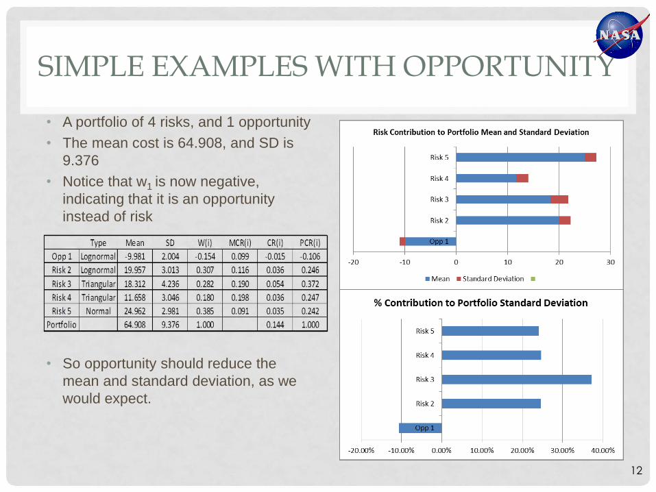
• A portfolio of 4 risks, and 1 opportunity

• The mean cost is 64.908, and SD is

9.376

• Notice that w1 is now negative,

indicating that it is an opportunity

instead of risk

Type Mean so W( i) MCR(i) CR(i) PCR( i)

Opp 1 Lognormal -9.981 2.004 -0.154 0.099 -0.015 -0.106

Risk 2 Lognormal 19.957 3.013 0.307 0.116 0.036 0.246

Risk 3 Triangular 18.312 4.236 0.282 0.190 0.054 0.372

Risk4 Triangu lar 11.658 3.046 0. 180 0.198 0.036 0.247

Risk 5 Normal 24.962 2.981 0.385 0.091 0.035 0.242

Portfolio 64.908 9.376 1.000 0.144 1.000

• So opportunity should reduce the

mean and standard deviation, as we

would expect.

12

HOW TO EXTEND TO SCHEDULE RISK

• What is a portfolio in a schedule sense?

• How do we define this portfolio in a project with many

tasks?

• Main measure is project duration, driven by critical path.

• Not every task contributes to critical path though all contributes to

overall costs.

• So a portfolio for schedule should only consists of tasks that are

on, or potentially will be on critical path.

• Make use of criticality index, a common output of many schedule

tools, to define critical tasks.

13

SCHEDULE EXAMPLES (1) WITH TASK UNCERTAINTIES ONLY

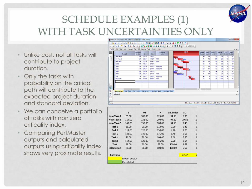
• Unlike cost, not all tasks will

contribute to project

duration.

• Only the tasks with

probability on the critical

path will contribute to the

expected project duration

and standard deviation.

• We can conceive a portfolio

of tasks with non zero

criticality index.

• Comparing PertMaster

outputs and calculated

outputs using criticality index

shows very proximate results.

L ML H Cri_index SD

New Task A 095.00 100.00 125.00 94.10 6.93 1

New Task B 5114.00 132.00 204.00 94.10 19.82 1

New Task C 5143.00 150.00 180.00 94.10 8.40 1

Task E 86.00 90.00 113.00 3.90 6.32 9

Task F 2114.00 120.00 150.00 4.20 8.25 1

Task G 4133.00 140.00 175.00 6.40 9.56 1

Task H 76.00 80.00 104.00 2.60 6.55 8

Task I 3114.00 120.00 156.00 2.20 9.64 1

Test 48.00 50.00 63.00 100.00 3.68 5

Integration 76.00 80.00 100.00 100.00 5.62 8

Portfolio 522.47 5

Model output

Calculated

Mean

Duration

Mean*

Cri_index

Sd*

Cri_index

6.67 100.38 6.52

0.00 141.15 18.65

7.66 148.36 7.90

6.33 3.76 0.25

8.00 5.38 0.35

9.33 9.56 0.61

6.67 2.25 0.17

0.00 2.86 0.21

3.67 53.67 3.68

5.34 85.34 5.62

3.00 552.70 22.33

14

SCHEDULE EXAMPLES (1) WITH TASK UNCERTAINTIES ONLY

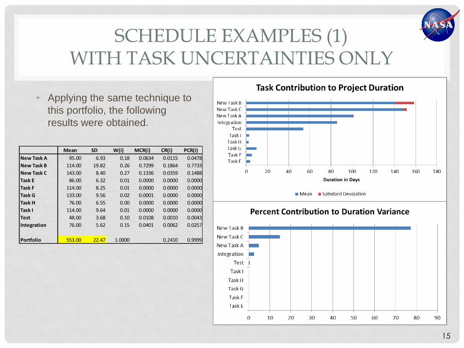
• Applying the same technique to

this portfolio, the following

results were obtained.

Mean SD W(i) MCR(i) CR(i) PCR(i)

New Task A 95.00 6.93 0.18 0.0634 0.0115 0.0478

New Task B 114.00 19.82 0.26 0.7299 0.1864 0.7733

New Task C 143.00 8.40 0.27 0.1336 0.0359 0.1488

Task E 86.00 6.32 0.01 0.0000 0.0000 0.0000

Task F 114.00 8.25 0.01 0.0000 0.0000 0.0000

Task G 133.00 9.56 0.02 0.0001 0.0000 0.0000

Task H 76.00 6.55 0.00 0.0000 0.0000 0.0000

Task I 114.00 9.64 0.01 0.0000 0.0000 0.0000

Test 48.00 3.68 0.10 0.0108 0.0010 0.0043

Integration 76.00 5.62 0.15 0.0401 0.0062 0.0257

Portfolio 553.00 22.47 1.0000 0.2410 0.9999

15

SCHEDULE EXAMPLES (2) WITH TASK UNCERTAINTIES PLUS RISKS

• In this case 2 discrete risks were added.

• Adding discrete risks changes the dynamics of the critical path.

• Discrete risks push Tasks E,F,G to be on the critical path.

• It is also important to note that discrete risks increases portfolio standard deviation substantially.

• For example, discrete risks increase expected duration by 9.2% but standard deviation by 59%.

• The increase in variance of discrete risks is due to binomial nature of probability of existence of risks.

L ML H Cri_index SD

Mean

Duration

Mean*

Cri_index

Sd*

Cri_index

New Task A 95 100 125 16.35 6.93

New Task B 114 132 204 16.35 19.83

New Task C 143 150 180 16.35 8.4

Task E 83.16 23.67

Task E 86 90 113 83.16 6.32

22.84risk 1 40 60 80 96.06

Task F 84.08 31.84

Task F 114 120 150 84.08

93.25

8.25

30.68risk 2 40 50 90

Task G 133 140 175 84.21 9.56

Task H 76 80 104 1.18 6.55

Task I 114 120 156 0.13 9.64

Test 48 50 63 100.00 3.68

Integration 76 80 100 100.00 5.62

Portfolio Model (

Calculate

106.67 17.44 1.13

150 24.53 3.24

157.67 25.78 1.37

147.37 0.00 19.68

96.33 80.11 5.26

51.04 49.03 21.94

164.07 0.00 26.77

128 107.62 6.94

36.07 33.64 28.61

149.33 125.75 8.05

86.67 1.02 0.08

130 0.17 0.01

53.67 53.67 3.68

85.33 85.33 5.62

MC) 604.00 35.50

d 604.08 35.04

16

SCHEDULE EXAMPLES (2) WITH TASK UNCERTAINTIES PLUS RISKS

17

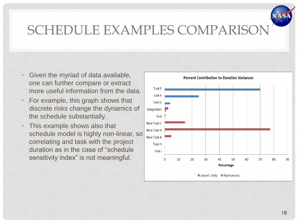
SCHEDULE EXAMPLES COMPARISON

• Given the myriad of data available,

one can further compare or extract

more useful information from the data.

• For example, this graph shows that

discrete risks change the dynamics of

the schedule substantially.

• This example shows also that

schedule model is highly non-linear, so

correlating and task with the project

duration as in the case of “schedule

sensitivity index” is not meaningful.

18

CONCLUSION AND FUTURE WORK

• A portfolio approach to risk attribution for cost and schedule risks, and the

mathematical framework has been developed.

• This risk attribution methodology can be extended to include cost “opportunity” in

reducing the expected cost and cost variance as one would expect.

• The same methodology can be extended to schedule risks by properly considering

only the tasks that affect the critical path as a portfolio.

• This algorithm provides a more precise risk impact quantification and disaggregation

so that each risk/uncertainty can be better quantified.

• The methodology is simple and can be incorporated easily into existing cost/schedule

simulation tools using mainly matrix operations.

• This algorithm has not been tested for more complex risk topology such as multiple

risks assigned to the same task, serial or parallel assignment of risks to the same

task.

• Therefore, future work will consider this more complex topology.

19