1

A Mathematical Theory of Deep ConvolutionalNeural Networks for Feature Extraction

Thomas Wiatowski and Helmut Bolcskei, Fellow, IEEE

Abstract—Deep convolutional neural networks have led tobreakthrough results in numerous practical machine learningtasks such as classification of images in the ImageNet dataset, control-policy-learning to play Atari games or the boardgame Go, and image captioning. Many of these applications firstperform feature extraction and then feed the results thereof intoa trainable classifier. The mathematical analysis of deep convo-lutional neural networks for feature extraction was initiated byMallat, 2012. Specifically, Mallat considered so-called scatteringnetworks based on a wavelet transform followed by the modulusnon-linearity in each network layer, and proved translationinvariance (asymptotically in the wavelet scale parameter) anddeformation stability of the corresponding feature extractor.This paper complements Mallat’s results by developing a theorythat encompasses general convolutional transforms, or in moretechnical parlance, general semi-discrete frames (including Weyl-Heisenberg filters, curvelets, shearlets, ridgelets, wavelets, andlearned filters), general Lipschitz-continuous non-linearities (e.g.,rectified linear units, shifted logistic sigmoids, hyperbolic tan-gents, and modulus functions), and general Lipschitz-continuouspooling operators emulating, e.g., sub-sampling and averaging.In addition, all of these elements can be different in differentnetwork layers. For the resulting feature extractor we prove atranslation invariance result of vertical nature in the sense ofthe features becoming progressively more translation-invariantwith increasing network depth, and we establish deformationsensitivity bounds that apply to signal classes such as, e.g., band-limited functions, cartoon functions, and Lipschitz functions.

Index Terms—Machine learning, deep convolutional neuralnetworks, scattering networks, feature extraction, frame theory.

I. INTRODUCTION

A central task in machine learning is feature extraction[2]–[4] as, e.g., in the context of handwritten digit

classification [5]. The features to be extracted in this casecorrespond, for example, to the edges of the digits. Theidea behind feature extraction is that feeding characteristicfeatures of the signals—rather than the signals themselves—toa trainable classifier (such as, e.g., a support vector machine(SVM) [6]) improves classification performance. Specifically,non-linear feature extractors (obtained, e.g., through the useof a so-called kernel in the context of SVMs) can map inputsignal space dichotomies that are not linearly separable intolinearly separable feature space dichotomies [3]. Sticking tothe example of handwritten digit classification, we would,moreover, want the feature extractor to be invariant to the

The authors are with the Department of Information Technologyand Electrical Engineering, ETH Zurich, 8092 Zurich, Switzerland.Email: withomas, boelcskei@nari.ee.ethz.ch

The material in this paper was presented in part at the 2015 IEEEInternational Symposium on Information Theory (ISIT), Hong Kong, China.

Copyright (c) 2017 IEEE. Personal use of this material is permitted.However, permission to use this material for any other purposes must beobtained from the IEEE by sending a request to pubs-permissions@ieee.org.

digits’ spatial location within the image, which leads tothe requirement of translation invariance. In addition, it isdesirable that the feature extractor be robust with respectto (w.r.t.) handwriting styles. This can be accomplished bydemanding limited sensitivity of the features to certain non-linear deformations of the signals to be classified.

Spectacular success in practical machine learning tasks hasbeen reported for feature extractors generated by so-calleddeep convolutional neural networks (DCNNs) [2], [7]–[11],[13], [14]. These networks are composed of multiple layers,each of which computes convolutional transforms, followedby non-linearities and pooling1 operators. While DCNNs canbe used to perform classification (or other machine learningtasks such as regression) directly [2], [7], [9]–[11], typicallybased on the output of the last network layer, they can also actas stand-alone feature extractors [15]–[21] with the resultingfeatures fed into a classifier such as a SVM. The present paperpertains to the latter philosophy.

The mathematical analysis of feature extractors generatedby DCNNs was pioneered by Mallat in [22]. Mallat’s the-ory applies to so-called scattering networks, where signalsare propagated through layers that compute a semi-discretewavelet transform (i.e., convolutions with filters that are ob-tained from a mother wavelet through scaling and rotationoperations), followed by the modulus non-linearity, withoutsubsequent pooling. The resulting feature extractor is shownto be translation-invariant (asymptotically in the scale param-eter of the underlying wavelet transform) and stable w.r.t.certain non-linear deformations. Moreover, Mallat’s scatteringnetworks lead to state-of-the-art results in various classificationtasks [23]–[25].

Contributions. DCNN-based feature extractors that werefound to work well in practice employ a wide range of i) filters,namely pre-specified structured filters such as wavelets [16],[19]–[21], pre-specified unstructured filters such as randomfilters [16], [17], and filters that are learned in a super-vised [15], [16] or an unsupervised [16]–[18] fashion, ii)non-linearities beyond the modulus function [16], [21], [22],namely hyperbolic tangents [15]–[17], rectified linear units[26], [27], and logistic sigmoids [28], [29], and iii) poolingoperators, namely sub-sampling [19], average pooling [15],[16], and max-pooling [16], [17], [20], [21]. In addition, thefilters, non-linearities, and pooling operators can be differentin different network layers [14]. The goal of this paper isto develop a mathematical theory that encompasses all theseelements (apart from max-pooling) in full generality.

1In the literature “pooling” broadly refers to some form of combining“nearby” values of a signal (e.g., through averaging) or picking one rep-resentative value (e.g, through maximization or sub-sampling).

arX

iv:1

512.

0629

3v3

[cs

.IT

] 2

4 O

ct 2

017

2

Convolutional transforms as employed in DCNNs canbe interpreted as semi-discrete signal transforms [30]–[37](i.e., convolutional transforms with filters that are countablyparametrized). Corresponding prominent representatives arecurvelet [34], [35], [38] and shearlet [36], [39] transforms,both of which are known to be highly effective in extract-ing features characterized by curved edges in images. Ourtheory allows for general semi-discrete signal transforms,general Lipschitz-continuous non-linearities (e.g., rectifiedlinear units, shifted logistic sigmoids, hyperbolic tangents,and modulus functions), and incorporates continuous-timeLipschitz pooling operators that emulate discrete-time sub-sampling and averaging. Finally, different network layersmay be equipped with different convolutional transforms,different (Lipschitz-continuous) non-linearities, and different(Lipschitz-continuous) pooling operators.

Regarding translation invariance, it was argued, e.g., in[15]–[17], [20], [21], that in practice invariance of the featuresis crucially governed by network depth and by the presence ofpooling operators (such as, e.g., sub-sampling [19], average-pooling [15], [16], or max-pooling [16], [17], [20], [21]). Weshow that the general feature extractor considered in this paper,indeed, exhibits such a vertical translation invariance and thatpooling plays a crucial role in achieving it. Specifically, weprove that the depth of the network determines the extent towhich the extracted features are translation-invariant. We alsoshow that pooling is necessary to obtain vertical translationinvariance as otherwise the features remain fully translation-covariant irrespective of network depth. We furthermore es-tablish a deformation sensitivity bound valid for signal classessuch as, e.g., band-limited functions, cartoon functions [40],and Lipschitz functions [40]. This bound shows that small non-linear deformations of the input signal lead to small changesin the corresponding feature vector.

In terms of mathematical techniques, we draw heavilyfrom continuous frame theory [41], [42]. We develop a proofmachinery that is completely detached from the structures2

of the semi-discrete transforms and the specific form of theLipschitz non-linearities and Lipschitz pooling operators. Theproof of our deformation sensitivity bound is based on two keyelements, namely Lipschitz continuity of the feature extractorand a deformation sensitivity bound for the signal class underconsideration, namely band-limited functions (as establishedin the present paper) or cartoon functions and Lipschitzfunctions as shown in [40]. This “decoupling” approach hasimportant practical ramifications as it shows that wheneverwe have deformation sensitivity bounds for a signal class,we automatically get deformation sensitivity bounds for theDCNN feature extractor operating on that signal class. Ourresults hence establish that vertical translation invariance andlimited sensitivity to deformations—for signal classes withinherent deformation insensitivity—are guaranteed by the net-work structure per se rather than the specific convolutionkernels, non-linearities, and pooling operators.

2Structure here refers to the structural relationship between the convolutionkernels in a given layer, e.g., scaling and rotation operations in the case ofthe wavelet transform.

Notation. The complex conjugate of z ∈ C is denoted byz. We write Re(z) for the real, and Im(z) for the imaginarypart of z ∈ C. The Euclidean inner product of x, y ∈ Cd is〈x, y〉 :=

∑di=1 xiyi, with associated norm |x| :=

√〈x, x〉.

We denote the identity matrix by E ∈ Rd×d. For the matrixM ∈ Rd×d, Mi,j designates the entry in its i-th row and j-th column, and for a tensor T ∈ Rd×d×d, Ti,j,k refers to its(i, j, k)-th component. The supremum norm of the matrix M ∈Rd×d is defined as |M |∞ := supi,j |Mi,j |, and the supremumnorm of the tensor T ∈ Rd×d×d is |T |∞ := supi,j,k |Ti,j,k|.We write Br(x) ⊆ Rd for the open ball of radius r > 0centered at x ∈ Rd. O(d) stands for the orthogonal group ofdimension d ∈ N, and SO(d) for the special orthogonal group.

For a Lebesgue-measurable function f : Rd → C, wewrite

∫Rd f(x)dx for the integral of f w.r.t. Lebesgue mea-

sure µL. For p ∈ [1,∞), Lp(Rd) stands for the spaceof Lebesgue-measurable functions f : Rd → C satisfying‖f‖p := (

∫Rd |f(x)|pdx)1/p <∞. L∞(Rd) denotes the space

of Lebesgue-measurable functions f : Rd → C such that‖f‖∞ := infα > 0 | |f(x)| ≤ α for a.e.3 x ∈ Rd < ∞.For f, g ∈ L2(Rd) we set 〈f, g〉 :=

∫Rd f(x)g(x)dx. For

R > 0, the space of R-band-limited functions is denotedas L2

R(Rd) := f ∈ L2(Rd) | supp(f) ⊆ BR(0). Fora countable set Q, (L2(Rd))Q stands for the space of setss := sqq∈Q, sq ∈ L2(Rd), for all q ∈ Q, satisfying|||s||| := (

∑q∈Q ‖sq‖22)1/2 <∞.

Id : Lp(Rd) → Lp(Rd) denotes the identity operator onLp(Rd). The tensor product of functions f, g : Rd → C is (f⊗g)(x, y) := f(x)g(y), (x, y) ∈ Rd×Rd. The operator norm ofthe bounded linear operator A : Lp(Rd)→ Lq(Rd) is definedas ‖A‖p,q := sup‖f‖p=1 ‖Af‖q . We denote the Fourier trans-form of f ∈ L1(Rd) by f(ω) :=

∫Rd f(x)e−2πi〈x,ω〉dx and

extend it in the usual way to L2(Rd) [43, Theorem 7.9]. Theconvolution of f ∈ L2(Rd) and g ∈ L1(Rd) is (f ∗ g)(y) :=∫Rd f(x)g(y− x)dx. We write (Ttf)(x) := f(x− t), t ∈ Rd,

for the translation operator, and (Mωf)(x) := e2πi〈x,ω〉f(x),ω ∈ Rd, for the modulation operator. Involution is defined by(If)(x) := f(−x).

A multi-index α = (α1, . . . , αd) ∈ Nd0 is an orderedd-tuple of non-negative integers αi ∈ N0. For a multi-index α ∈ Nd0, Dα denotes the differential operator Dα :=(∂/∂x1)α1 . . . (∂/∂xd)

αd , with order |α| :=∑di=1 αi. If

|α| = 0, Dαf := f , for f : Rd → C. The space of functionsf : Rd → C whose derivatives Dαf of order at most N ∈ N0

are continuous is designated by CN (Rd,C), and the spaceof infinitely differentiable functions is C∞(Rd,C). S(Rd,C)stands for the Schwartz space, i.e., the space of functionsf ∈ C∞(Rd,C) whose derivatives Dαf along with the func-tion itself are rapidly decaying [43, Section 7.3] in the senseof sup|α|≤N supx∈Rd(1+|x|2)N |(Dαf)(x)| <∞, for all N ∈N0. We denote the gradient of a function f : Rd → C as ∇f .The space of continuous mappings v : Rp → Rq is C(Rp,Rq),and for k, p, q ∈ N, the space of k-times continuously differ-entiable mappings v : Rp → Rq is written as Ck(Rp,Rq).For a mapping v : Rd → Rd, we let Dv be its Jacobianmatrix, and D2v its Jacobian tensor, with associated norms

3Throughout “a.e.” is w.r.t. Lebesgue measure.

3

‖v‖∞ := supx∈Rd |v(x)|, ‖Dv‖∞ := supx∈Rd |(Dv)(x)|∞,and ‖D2v‖∞ := supx∈Rd |(D2v)(x)|∞.

II. SCATTERING NETWORKS

We set the stage by reviewing scattering networks as intro-duced in [22], the basis of which is a multi-layer architecturethat involves a wavelet transform followed by the modulusnon-linearity, without subsequent pooling. Specifically, [22,Definition 2.4] defines the feature vector ΦW (f) of the signalf ∈ L2(Rd) as the set4

ΦW (f) :=

∞⋃n=0

ΦnW (f), (1)

where Φ0W (f) := f ∗ ψ(−J,0), and

ΦnW (f)

:=

(U[λ

(j)

, . . . , λ(p)︸ ︷︷ ︸

n indices

]f)∗ ψ(−J,0)

λ(j),...,λ

(p)∈ΛW\(−J,0),

for all n ∈ N, with

U[λ

(j)

, . . . , λ(p)]

f :=∣∣ · · · ∣∣ |f ∗ ψ

λ(j) | ∗ ψ

λ(k)

∣∣ · · · ∗ ψλ(p)

∣∣︸ ︷︷ ︸n−fold convolution followed by modulus

.

Here, the index set ΛW :=

(−J, 0)∪

(j, k) | j ∈Z with j > −J, k ∈ 0, . . . ,K−1

contains pairs of scales

j and directions k (in fact, k is the index of the directiondescribed by the rotation matrix rk), and

ψλ(x) := 2djψ(2jr−1k x), (2)

where λ = (j, k) ∈ ΛW\(−J, 0) are directional wavelets[30], [44], [45] with (complex-valued) mother wavelet ψ ∈L1(Rd) ∩ L2(Rd). The rk, k ∈ 0, . . . ,K − 1, are elementsof a finite rotation group G (if d is even, G is a subgroupof SO(d); if d is odd, G is a subgroup of O(d)). The index(−J, 0) ∈ ΛW is associated with the low-pass filter ψ(−J,0) ∈L1(Rd)∩L2(Rd), and J ∈ Z corresponds to the coarsest scaleresolved by the directional wavelets (2).

The family of functions ψλλ∈ΛW is taken to form a semi-discrete Parseval frame

ΨΛW := TbIψλb∈Rd,λ∈ΛW,

for L2(Rd) [30], [41], [42] and hence satisfies∑λ∈ΛW

∫Rd

|〈f, TbIψλ〉|2db =∑λ∈ΛW

‖f ∗ ψλ‖22 = ‖f‖22,

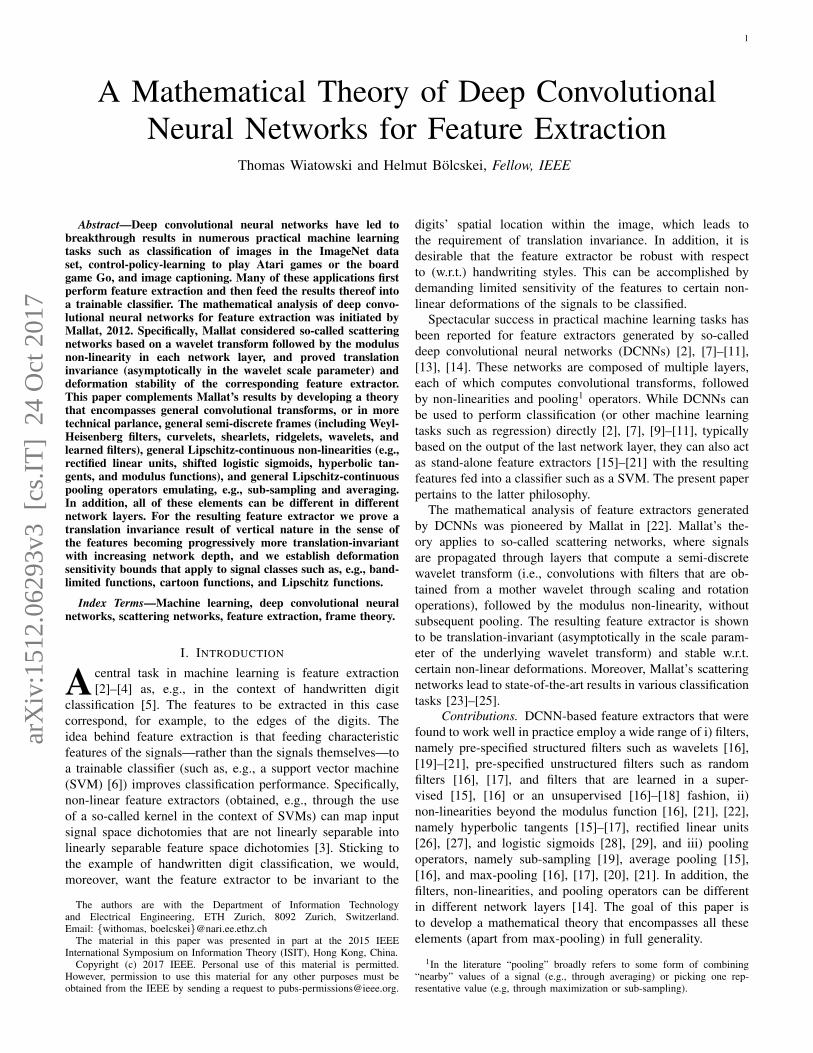
for all f ∈ L2(Rd), where 〈f, TbIψλ〉 = (f ∗ ψλ)(b),(λ, b) ∈ ΛW × Rd, are the underlying frame coefficients.Note that for given λ ∈ ΛW, we actually have a continuumof frame coefficients as the translation parameter b ∈ Rd isleft unsampled. We refer to Figure 1 for a frequency-domainillustration of a semi-discrete directional wavelet frame. InAppendix A, we give a brief review of the general theory ofsemi-discrete frames, and in Appendices B and C we collectstructured example frames in 1-D and 2-D, respectively.

4We emphasize that the feature vector ΦW (f) is a union of the sets offeature vectors ΦnW (f).

ω1

ω2

Fig. 1: Partitioning of the frequency plane R2 induced by a semi-discretedirectional wavelet frame with K = 12 directions.

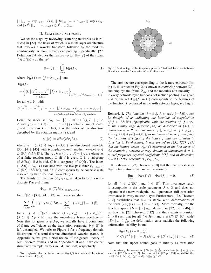
The architecture corresponding to the feature extractor ΦWin (1), illustrated in Fig. 2, is known as scattering network [22],and employs the frame ΨΛW and the modulus non-linearity | · |in every network layer, but does not include pooling. For givenn ∈ N, the set ΦnW (f) in (1) corresponds to the features ofthe function f generated in the n-th network layer, see Fig. 2.

Remark 1. The function |f ∗ ψλ|, λ ∈ ΛW\(−J, 0), canbe thought of as indicating the locations of singularitiesof f ∈ L2(Rd). Specifically, with the relation of |f ∗ ψλ|to the Canny edge detector [46] as described in [31], indimension d = 2, we can think of |f ∗ ψλ| = |f ∗ ψ(j,k)|,λ = (j, k) ∈ ΛW\(−J, 0), as an image at scale j specifyingthe locations of edges of the image f that are oriented indirection k. Furthermore, it was argued in [23], [25], [47]that the feature vector Φ1

W (f) generated in the first layer ofthe scattering network is very similar, in dimension d = 1,to mel frequency cepstral coefficients [48], and in dimensiond = 2 to SIFT-descriptors [49], [50].

It is shown in [22, Theorem 2.10] that the feature extractorΦW is translation-invariant in the sense of

limJ→∞

|||ΦW (Ttf)− ΦW (f)||| = 0, (3)

for all f ∈ L2(Rd) and t ∈ Rd. This invariance resultis asymptotic in the scale parameter J ∈ Z and does notdepend on the network depth, i.e., it guarantees full translationinvariance in every network layer. Furthermore, [22, Theorem2.12] establishes that ΦW is stable w.r.t. deformations ofthe form (Fτf)(x) := f(x − τ(x)). More formally, for thefunction space (HW , ‖ · ‖HW

) defined in [22, Eq. 2.46], itis shown in [22, Theorem 2.12] that there exists a constantC > 0 such that for all f ∈ HW , and τ ∈ C1(Rd,Rd) with5

‖Dτ‖∞ ≤ 12d , the deformation error satisfies the following

deformation stability bound

|||ΦW (Fτf)− ΦW (f)|||≤ C

(2−J‖τ‖∞ + J‖Dτ‖∞ + ‖D2τ‖∞

)‖f‖HW

. (4)

Note that this upper bound goes to infinity as translation

5It is actually the assumption ‖Dτ‖∞ ≤ 12d

, rather than ‖Dτ‖∞ ≤ 12

asstated in [22, Theorem 2.12], that is needed in [22, p. 1390] to establish that|det(E − (Dτ)(x))| ≥ 1− d‖Dτ‖∞ ≥ 1/2.

4

f

|f ∗ ψλ(j) |

|f ∗ ψλ(j) | ∗ ψ(−J,0)

||f ∗ ψλ(j) | ∗ ψ

λ(l) |

||f ∗ ψλ(j) | ∗ ψ

λ(l) | ∗ ψ(−J,0)

|||f ∗ ψλ(j) | ∗ ψ

λ(l) | ∗ ψ

λ(m) |

· · ·

|f ∗ ψλ(p) |

|f ∗ ψλ(p) | ∗ ψ(−J,0)

||f ∗ ψλ(p) | ∗ ψ

λ(r) |

||f ∗ ψλ(p) | ∗ ψ

λ(r) | ∗ ψ(−J,0)

|||f ∗ ψλ(p) | ∗ ψ

λ(r) | ∗ ψ

λ(s) |

· · ·

f ∗ ψ(−J,0)

Fig. 2: Scattering network architecture based on wavelet filters and the modulus non-linearity. The elements of the feature vector ΦW (f) in (1) are indicatedat the tips of the arrows.

invariance through J → ∞ is induced. In practice sig-nal classification based on scattering networks is performedas follows. First, the function f and the wavelet frameatoms ψλλ∈ΛW are discretized to finite-dimensional vectors.The resulting scattering network then computes the finite-dimensional feature vector ΦW (f), whose dimension is typ-ically reduced through an orthogonal least squares step [51],and then feeds the result into a trainable classifier such as, e.g.,a SVM. State-of-the-art results for scattering networks werereported for various classification tasks such as handwrittendigit recognition [23], texture discrimination [23], [24], andmusical genre classification [25].

III. GENERAL DEEP CONVOLUTIONALFEATURE EXTRACTORS

As already mentioned, scattering networks follow the ar-chitecture of DCNNs [2], [7]–[11], [15]–[21] in the senseof cascading convolutions (with atoms ψλλ∈ΛW of thewavelet frame ΨΛW ) and non-linearities, namely the modulusfunction, but without pooling. General DCNNs as studied inthe literature exhibit a number of additional features:

– a wide variety of filters are employed, namely pre-specified unstructured filters such as random filters [16],[17], and filters that are learned in a supervised [15], [16]or an unsupervised [16]–[18] fashion.

– a wide variety of non-linearities are used such as, e.g.,hyperbolic tangents [15]–[17], rectified linear units [26],[27], and logistic sigmoids [28], [29].

– convolution and the application of a non-linearity istypically followed by a pooling operator such as, e.g.,sub-sampling [19], average-pooling [15], [16], or max-pooling [16], [17], [20], [21].

– the filters, non-linearities, and pooling operators are al-lowed to be different in different network layers [11],[14].

As already mentioned, the purpose of this paper is to developa mathematical theory of DCNNs for feature extraction thatencompasses all of the aspects above (apart from max-pooling)with the proviso that the pooling operators we analyze arecontinuous-time emulations of discrete-time pooling operators.Formally, compared to scattering networks, in the n-th networklayer, we replace the wavelet-modulus operation |f ∗ ψλ| bya convolution with the atoms gλn ∈ L1(Rd) ∩ L2(Rd) of ageneral semi-discrete frame Ψn := TbIgλnb∈Rd,λn∈Λn

forL2(Rd) with countable index set Λn (see Appendix A for abrief review of the theory of semi-discrete frames), followedby a non-linearity Mn : L2(Rd) → L2(Rd) that satisfies theLipschitz property ‖Mnf − Mnh‖2 ≤ Ln‖f − h‖2, for allf, h ∈ L2(Rd), and Mnf = 0 for f = 0. The output of thisnon-linearity, Mn(f ∗ gλn

), is then pooled according to

f 7→ Sd/2n Pn(f)(Sn·), (5)

where Sn ≥ 1 is the pooling factor and Pn : L2(Rd) →L2(Rd) satisfies the Lipschitz property ‖Pnf − Pnh‖2 ≤Rn‖f − h‖2, for all f, h ∈ L2(Rd), and Pnf = 0 forf = 0. We next comment on the individual elements in ournetwork architecture in more detail. The frame atoms gλn arearbitrary and can, therefore, also be taken to be structured,e.g., Weyl-Heisenberg functions, curvelets, shearlets, ridgelets,or wavelets as considered in [22] (where the atoms gλn

areobtained from a mother wavelet through scaling and rotationoperations, see Section II). The corresponding semi-discretesignal transforms6, briefly reviewed in Appendices B and C,

6Let gλλ∈Λ ⊆ L1(Rd) ∩ L2(Rd) be a set of functions indexed bya countable set Λ. Then, the mapping f 7→ f ∗ gλ(b)b∈Rd,λ∈Λ =

〈f, TbIgλ〉λ∈Λ, f ∈ L2(Rd), is called a semi-discrete signal transform,as it depends on discrete indices λ ∈ Λ and continuous variables b ∈ Rd.We can think of this mapping as the analysis operator in frame theory [53],with the proviso that for given λ ∈ Λ, we actually have a continuum of framecoefficients as the translation parameter b ∈ Rd is left unsampled.

5

have been employed successfully in the literature in variousfeature extraction tasks [32], [54]–[61], but their use—apartfrom wavelets—in DCNNs appears to be new. We refer thereader to Appendix D for a detailed discussion of severalrelevant example non-linearities (e.g., rectified linear units,shifted logistic sigmoids, hyperbolic tangents, and, of course,the modulus function) that fit into our framework. We nextexplain how the continuous-time pooling operator (5) emulatesdiscrete-time pooling by sub-sampling [19] or by averaging[15], [16]. Consider a one-dimensional discrete-time signalfd ∈ `2(Z) := fd : Z → C |

∑k∈Z |fd[k]|2 < ∞. Sub-

sampling by a factor of S ∈ N in discrete time is defined by[62, Sec. 4]

fd 7→ hd := fd[S·]

and amounts to simply retaining every S-th sample of fd. Thediscrete-time Fourier transform of hd is given by a summationover translated and dilated copies of fd according to [62, Sec.4]

hd(θ) :=∑k∈Z

hd[k]e−2πikθ =1

S

S−1∑k=0

fd

(θ − kS

). (6)

The translated copies of fd in (6) are a consequence ofthe 1-periodicity of the discrete-time Fourier transform. Wetherefore emulate the discrete-time sub-sampling operation incontinuous time through the dilation operation

f 7→ h := Sd/2f(S·), f ∈ L2(Rd), (7)

which in the frequency domain amounts to dilation accordingto h = S−d/2f(S−1·). The scaling by Sd/2 in (7) ensuresunitarity of the continuous-time sub-sampling operation. Theoverall operation in (7) fits into our general definition ofpooling as it can be recovered from (5) simply by taking P toequal the identity mapping (which is, of course, Lipschitz-continuous with Lipschitz constant R = 1 and satisfiesIdf = 0 for f = 0). Next, we consider average pooling. Indiscrete time average pooling is defined by

fd 7→ hd := (fd ∗ φd)[S·] (8)

for the (typically compactly supported) “averaging kernel”φd ∈ `2(Z) and the averaging factor S ∈ N. Taking φd tobe a box function of length S amounts to computing localaverages of S consecutive samples. Weighted averages areobtained by identifying the desired weights with the averagingkernel φd. The operation (8) can be emulated in continuoustime according to

f 7→ Sd/2(f ∗ φ

)(S·), f ∈ L2(Rd), (9)

with the averaging window φ ∈ L1(Rd) ∩ L2(Rd). We notethat (9) can be recovered from (5) by taking P (f) = f ∗ φ,f ∈ L2(Rd), and noting that convolution with φ is Lipschitz-continuous with Lipschitz constant R = ‖φ‖1 (thanks toYoung’s inequality [63, Theorem 1.2.12]) and trivially satisfiesPf = 0 for f = 0. In the remainder of the paper, we referto the operation in (5) as Lipschitz pooling through dilationto indicate that (5) essentially amounts to the application of aLipschitz-continuous mapping followed by a continuous-time

dilation. Note, however, that the operation in (5) will not beunitary in general.

We next state definitions and collect preliminary resultsneeded for the analysis of the general DCNN feature extractorconsidered. The basic building blocks of this network arethe triplets (Ψn,Mn, Pn) associated with individual networklayers n and referred to as modules.

Definition 1. For n ∈ N, let Ψn = TbIgλnb∈Rd,λn∈Λnbe

a semi-discrete frame for L2(Rd) and let Mn : L2(Rd) →L2(Rd) and Pn : L2(Rd) → L2(Rd) be Lipschitz-continuousoperators with Mnf = 0 and Pnf = 0 for f = 0, respectively.Then, the sequence of triplets

Ω :=((Ψn,Mn, Pn)

)n∈N

is referred to as a module-sequence.

The following definition introduces the concept of paths onindex sets, which will prove useful in formalizing the featureextraction network. The idea for this formalism is due to [22].

Definition 2. Let Ω =((Ψn,Mn, Pn)

)n∈N be a module-

sequence, let gλnλn∈Λn be the atoms of the frame Ψn, andlet Sn ≥ 1 be the pooling factor (according to (5)) associatedwith the n-th network layer. Define the operator Un associatedwith the n-th layer of the network as Un : Λn × L2(Rd) →L2(Rd),

Un(λn, f) := Un[λn]f := Sd/2n Pn(Mn(f ∗gλn

))(Sn·). (10)

For n ∈ N, define the set Λn1 := Λ1 × Λ2 × · · · × Λn. Anordered sequence q = (λ1, λ2, . . . , λn) ∈ Λn1 is called a path.For the empty path e := ∅ we set Λ0

1 := e and U0[e]f := f ,for all f ∈ L2(Rd).

The operator Un is well-defined, i.e., Un[λn]f ∈ L2(Rd),for all (λn, f) ∈ Λn × L2(Rd), thanks to

‖Un[λn]f‖22 = Sdn

∫Rd

∣∣∣Pn(Mn(f ∗ gλn))(Snx)

∣∣∣2dx

=

∫Rd

∣∣∣Pn(Mn(f ∗ gλn))(y)∣∣∣2dy

= ‖Pn(Mn(f ∗ gλn

))‖22 ≤ R2

n‖Mn(f ∗ gλn)‖22 (11)

≤ L2nR

2n‖f ∗ gλn

‖22 ≤ BnL2nR

2n‖f‖22. (12)

For the inequality in (11) we used the Lipschitz continuityof Pn according to ‖Pnf − Pnh‖22 ≤ R2

n‖f − h‖22, togetherwith Pnh = 0 for h = 0 to get ‖Pnf‖22 ≤ R2

n‖f‖22. Similararguments lead to the first inequality in (12). The last step in(12) is thanks to

‖f ∗ gλn‖22 ≤∑

λ′n∈Λn

‖f ∗ gλ′n‖22 ≤ Bn‖f‖22,

which follows from the frame condition (30) on Ψn. We willalso need the extension of the operator Un to paths q ∈ Λn1according to

U [q]f =U [(λ1, λ2, . . . , λn)]f

:=Un[λn] · · ·U2[λ2]U1[λ1]f, (13)

with U [e]f := f . Note that the multi-stage operation (13) is

6

U [e]f = f

U[λ

(j)1

]f

(U[λ

(j)1

]f)∗ χ1

U[(λ

(j)1 , λ

(l)2

)]f

(U[(λ

(j)1 , λ

(l)2

)]f)∗ χ2

U[(λ

(j)1 , λ

(l)2 , λ

(m)3

)]f

· · ·

U[λ

(p)1

]f

(U[λ

(p)1

]f)∗ χ1

U[(λ

(p)1 , λ

(r)2

)]f

(U[(λ

(p)1 , λ

(r)2

)]f)∗ χ2

U[(λ

(p)1 , λ

(r)2 , λ

(s)3

)]f

· · ·

f ∗ χ0

Fig. 3: Network architecture underlying the general DCNN feature extractor. The index λ(k)n corresponds to the k-th atom g

λ(k)n

of the frame Ψn associatedwith the n-th network layer. The function χn is the output-generating atom of the n-th layer.

again well-defined thanks to

‖U [q]f‖22 ≤

(n∏k=1

BkL2kR

2k

)‖f‖22, (14)

for q ∈ Λn1 and f ∈ L2(Rd), which follows by repeatedapplication of (12).

In scattering networks one atom ψλ, λ ∈ ΛW, in thewavelet frame ΨΛW , namely the low-pass filter ψ(−J,0), issingled out to generate the extracted features according to (1),see also Fig. 2. We follow this construction and designateone of the atoms in each frame in the module-sequenceΩ =

((Ψn,Mn, Pn)

)n∈N as the output-generating atom

χn−1 := gλ∗n , λ∗n ∈ Λn, of the (n − 1)-th layer. The atomsgλnλn∈Λn\λ∗n ∪ χn−1 in Ψn are thus used across two

consecutive layers in the sense of χn−1 = gλ∗n generatingthe output in the (n − 1)-th layer, and the gλn

λn∈Λn\λ∗npropagating signals from the (n − 1)-th layer to the n-thlayer according to (10), see Fig. 3. Note, however, that ourtheory does not require the output-generating atoms to below-pass filters7. From now on, with slight abuse of notation,we shall write Λn for Λn\λ∗n as well. Finally, we notethat extracting features in every network layer via an output-generating atom can be regarded as employing skip-layerconnections [13], which skip network layers further down andfeed the propagated signals into the feature vector.

We are now ready to define the feature extractor ΦΩ basedon the module-sequence Ω.

Definition 3. Let Ω =((Ψn,Mn, Pn)

)n∈N be a module-

sequence. The feature extractor ΦΩ based on Ω maps L2(Rd)

7It is evident, though, that the actual choices of the output-generating atomswill have an impact on practical performance.

to its feature vector

ΦΩ(f) :=

∞⋃n=0

ΦnΩ(f), (15)

where ΦnΩ(f) := (U [q]f) ∗ χnq∈Λn1

, for all n ∈ N.

The set ΦnΩ(f) in (15) corresponds to the features of thefunction f generated in the n-th network layer, see Fig.3, where n = 0 corresponds to the root of the network.The feature extractor ΦΩ : L2(Rd) → (L2(Rd))Q, withQ :=

⋃∞n=0 Λn1 , is well-defined, i.e., ΦΩ(f) ∈ (L2(Rd))Q, for

all f ∈ L2(Rd), under a technical condition on the module-sequence Ω formalized as follows.

Proposition 1. Let Ω =((Ψn,Mn, Pn)

)n∈N be a module-

sequence. Denote the frame upper bounds of Ψn by Bn > 0and the Lipschitz constants of the operators Mn and Pn byLn > 0 and Rn > 0, respectively. If

maxBn, BnL2nR

2n ≤ 1, ∀n ∈ N, (16)

then the feature extractor ΦΩ : L2(Rd)→ (L2(Rd))Q is well-defined, i.e., ΦΩ(f) ∈ (L2(Rd))Q, for all f ∈ L2(Rd).

Proof. The proof is given in Appendix E.

As condition (16) is of central importance, we formalize itas follows.

Definition 4. Let Ω =((Ψn,Mn, Pn)

)n∈N be a module-

sequence with frame upper bounds Bn > 0 and Lipschitzconstants Ln, Rn > 0 of the operators Mn and Pn, respec-tively. The condition

maxBn, BnL2nR

2n ≤ 1, ∀n ∈ N, (17)

is referred to as admissibility condition. Module-sequencesthat satisfy (17) are called admissible.

7

(a) (b) (c)

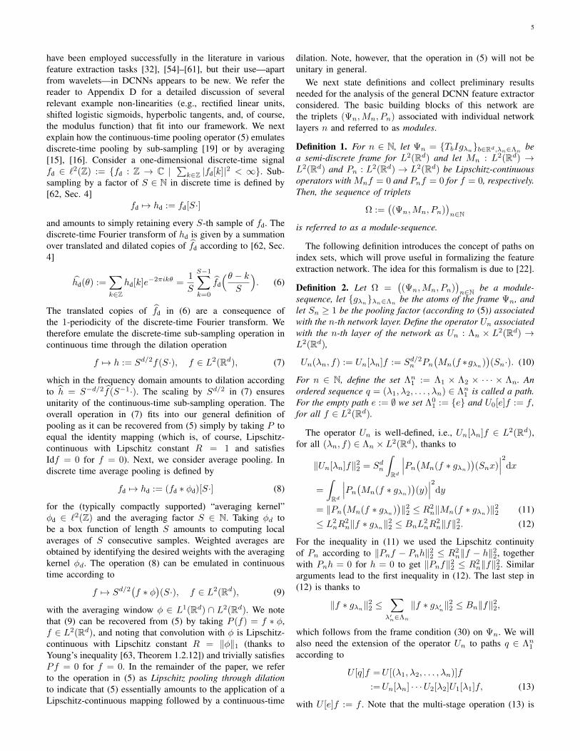
Fig. 4: Handwritten digits from the MNIST data set [5]. For practical machine learning tasks (e.g., signal classification), we often want the feature vectorΦΩ(f) to be invariant to the digits’ spatial location within the image f . Theorem 1 establishes that the features ΦnΩ(f) become more translation-invariantwith increasing layer index n.

We emphasize that condition (17) is easily met in practice.To see this, first note that Bn is determined through the frameΨn (e.g., the directional wavelet frame introduced in SectionII has B = 1), Ln is set through the non-linearity Mn (e.g.,the modulus function M = | · | has L = 1, see Appendix D),and Rn depends on the operator Pn in (5) (e.g., pooling bysub-sampling amounts to P = Id and has R = 1). Obviously,condition (17) is met if

Bn ≤ min1, L−2n R−2

n , ∀n ∈ N,

which can be satisfied by simply normalizing the frameelements of Ψn accordingly. We refer to Proposition 3 in Ap-pendix A for corresponding normalization techniques, which,as explained in Section IV, affect neither our translationinvariance result nor our deformation sensitivity bounds.

IV. PROPERTIES OF THE FEATURE EXTRACTOR ΦΩ

A. Vertical translation invariance

The following theorem states that under very mild de-cay conditions on the Fourier transforms χn of the output-generating atoms χn, the feature extractor ΦΩ exhibits verticaltranslation invariance in the sense of the features becomingmore translation-invariant with increasing network depth. Thisresult is in line with observations made in the deep learningliterature, e.g., in [15]–[17], [20], [21], where it is informallyargued that the network outputs generated at deeper layers tendto be more translation-invariant.

Theorem 1. Let Ω =((Ψn,Mn, Pn)

)n∈N be an admissible

module-sequence, let Sn ≥ 1, n ∈ N, be the pooling factors in(10), and assume that the operators Mn : L2(Rd)→ L2(Rd)and Pn : L2(Rd) → L2(Rd) commute with the translationoperator Tt, i.e.,

MnTtf = TtMnf, PnTtf = TtPnf, (18)

for all f ∈ L2(Rd), t ∈ Rd, and n ∈ N.

i) The features ΦnΩ(f) generated in the n-th network layersatisfy

ΦnΩ(Ttf) = Tt/(S1···Sn)ΦnΩ(f), (19)

for all f ∈ L2(Rd), t ∈ Rd, and n ∈ N, where TtΦnΩ(f)refers to element-wise application of Tt, i.e., TtΦnΩ(f) :=Tth | ∀h ∈ ΦnΩ(f).

ii) If, in addition, there exists a constant K > 0 (thatdoes not depend on n) such that the Fourier transformsχn of the output-generating atoms χn satisfy the decaycondition

|χn(ω)||ω| ≤ K, a.e. ω ∈ Rd, ∀n ∈ N0, (20)

then

|||ΦnΩ(Ttf)− ΦnΩ(f)||| ≤ 2π|t|KS1 · · ·Sn

‖f‖2, (21)

for all f ∈ L2(Rd) and t ∈ Rd.

Proof. The proof is given in Appendix F.

We start by noting that all pointwise (also referred to asmemoryless in the signal processing literature) non-linearitiesMn : L2(Rd) → L2(Rd) satisfy the commutation relation in(18). A large class of non-linearities widely used in the deeplearning literature, such as rectified linear units, hyperbolictangents, shifted logistic sigmoids, and the modulus func-tion as employed in [22], are, indeed, pointwise and hencecovered by Theorem 1. Moreover, P = Id as in poolingby sub-sampling trivially satisfies (18). Pooling by averagingPf = f ∗ φ, with φ ∈ L1(Rd) ∩ L2(Rd), satisfies (18) as aconsequence of the convolution operator commuting with thetranslation operator Tt.

Note that (20) can easily be met by taking the output-generating atoms χnn∈N0

either to satisfy

supn∈N0

‖χn‖1 + ‖∇χn‖1 <∞,

see, e.g., [43, Ch. 7], or to be uniformly band-limited in thesense of supp(χn) ⊆ Br(0), for all n ∈ N0, with an r that isindependent of n (see, e.g., [30, Ch. 2.3]). The bound in (21)shows that we can explicitly control the amount of translationinvariance via the pooling factors Sn. This result is in line withobservations made in the deep learning literature, e.g., in [15]–[17], [20], [21], where it is informally argued that pooling iscrucial to get translation invariance of the extracted features.Furthermore, the condition lim

n→∞S1 ·S2 · . . . ·Sn =∞ (easily

met by taking Sn > 1, for all n ∈ N) guarantees, thanks to(21), asymptotically full translation invariance according to

limn→∞

|||ΦnΩ(Ttf)− ΦnΩ(f)||| = 0, (22)

for all f ∈ L2(Rd) and t ∈ Rd. This means that the features

8

(a) (b) (c)

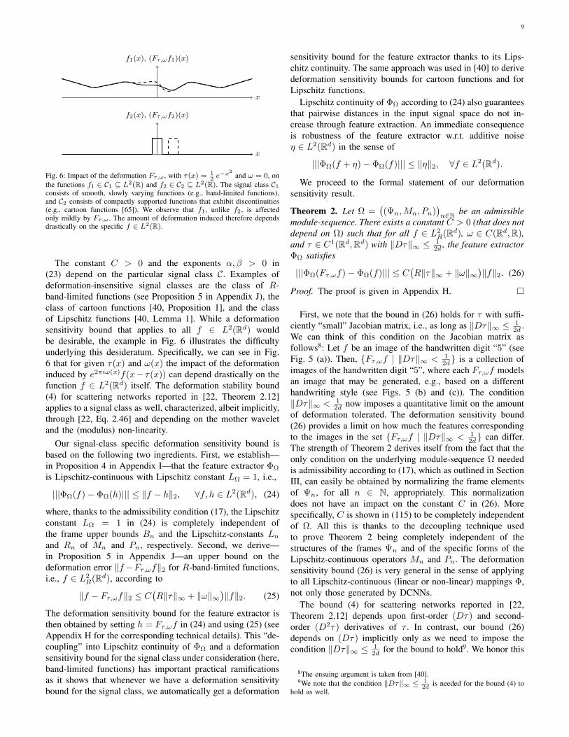
Fig. 5: Handwritten digits from the MNIST data set [5]. If f denotes the image of the handwritten digit “5” in (a), then—for appropriately chosen τ—thefunction Fτf = f(· − τ(·)) models images of “5” based on different handwriting styles as in (b) and (c).

ΦnΩ(Ttf) corresponding to the shifted versions Ttf of thehandwritten digit “3” in Figs. 4 (b) and (c) with increasingnetwork depth increasingly “look like” the features ΦnΩ(f)corresponding to the unshifted handwritten digit in Fig. 4(a). Casually speaking, the shift operator Tt is increasinglyabsorbed by ΦnΩ as n → ∞, with the upper bound (21)quantifying this absorption.

In contrast, the translation invariance result (3) in [22] isasymptotic in the wavelet scale parameter J , and does notdepend on the network depth, i.e., it guarantees full translationinvariance in every network layer. We honor this difference byreferring to (3) as horizontal translation invariance and to (22)as vertical translation invariance.

We emphasize that vertical translation invariance is a struc-tural property. Specifically, if Pn is unitary (such as, e.g., inthe case of pooling by sub-sampling where Pn simply equalsthe identity mapping), then so is the pooling operation in (5)owing to

‖Sd/2n Pn(f)(Sn·)‖22 = Sdn

∫Rd

|Pn(f)(Snx)|2dx

=

∫Rd

|Pn(f)(x)|2dx = ‖Pn(f)‖22 = ‖f‖22,

where we employed the change of variables y = Snx,dydx = Sdn. Regarding average pooling, as already mentioned,the operators Pn(f) = f ∗ φn, f ∈ L2(Rd), n ∈ N, are,in general, not unitary, but we still get translation invarianceas a consequence of structural properties, namely translationcovariance of the convolution operator combined with unitarydilation according to (7).

Finally, we note that in practice in certain applications itis actually translation covariance in the sense of ΦnΩ(Ttf) =TtΦ

nΩ(f), for all f ∈ L2(Rd) and t ∈ Rd, that is desirable,

for example, in facial landmark detection where the goal is toestimate the absolute position of facial landmarks in images. Insuch applications features in the layers closer to the root of thenetwork are more relevant as they are less translation-invariantand more translation-covariant. The reader is referred to [64]where corresponding numerical evidence is provided. Weproceed to the formal statement of our translation covarianceresult.

Corollary 1. Let Ω =((Ψn,Mn, Pn)

)n∈N be an admissible

module-sequence, let Sn ≥ 1, n ∈ N, be the pooling factors in(10), and assume that the operators Mn : L2(Rd)→ L2(Rd)

and Pn : L2(Rd) → L2(Rd) commute with the translationoperator Tt in the sense of (18). If, in addition, there existsa constant K > 0 (that does not depend on n) such thatthe Fourier transforms χn of the output-generating atoms χnsatisfy the decay condition (20), then

|||ΦnΩ(Ttf)− TtΦnΩ(f)||| ≤ 2π|t|K∣∣1/(S1 . . . Sn)− 1

∣∣‖f‖2,for all f ∈ L2(Rd) and t ∈ Rd.

Proof. The proof is given in Appendix G.

Corollary 1 shows that in the absence of pooling, i.e., takingSn = 1, for all n ∈ N, leads to full translation covariancein every network layer. This proves that pooling is necessaryto get vertical translation invariance as otherwise the featuresremain fully translation-covariant irrespective of the networkdepth. Finally, we note that scattering networks [22] (whichdo not employ pooling operators, see Section II) are renderedhorizontally translation-invariant by letting the wavelet scaleparameter J →∞.

B. Deformation sensitivity bound

The next result provides a bound—for band-limited signalsf ∈ L2

R(Rd)—on the sensitivity of the feature extractor ΦΩ

w.r.t. time-frequency deformations of the form

(Fτ,ωf)(x) := e2πiω(x)f(x− τ(x)).

This class of deformations encompasses non-linear distortionsf(x − τ(x)) as illustrated in Fig. 5, and modulation-likedeformations e2πiω(x)f(x) which occur, e.g., if the signal fis subject to an undesired modulation and we therefore haveaccess to a bandpass version of f only.

The deformation sensitivity bound we derive is signal-classspecific in the sense of applying to input signals belonging toa particular class, here band-limited functions. The proof tech-nique we develop applies, however, to all signal classes thatexhibit “inherent” deformation insensitivity in the followingsense.

Definition 5. A signal class C ⊆ L2(Rd) is calleddeformation-insensitive if there exist α, β, C > 0 such thatfor all f ∈ C, ω ∈ C(Rd,R), and (possibly non-linear)τ ∈ C1(Rd,Rd) with ‖Dτ‖∞ ≤ 1

2d , it holds that

‖f − Fτ,ωf‖2 ≤ C(‖τ‖α∞ + ‖ω‖β∞

). (23)

9

x

f1(x), (Fτ,ωf1)(x)

x

f2(x), (Fτ,ωf2)(x)

Fig. 6: Impact of the deformation Fτ,ω , with τ(x) = 12e−x

2and ω = 0, on

the functions f1 ∈ C1 ⊆ L2(R) and f2 ∈ C2 ⊆ L2(R). The signal class C1consists of smooth, slowly varying functions (e.g., band-limited functions),and C2 consists of compactly supported functions that exhibit discontinuities(e.g., cartoon functions [65]). We observe that f1, unlike f2, is affectedonly mildly by Fτ,ω . The amount of deformation induced therefore dependsdrastically on the specific f ∈ L2(R).

The constant C > 0 and the exponents α, β > 0 in(23) depend on the particular signal class C. Examples ofdeformation-insensitive signal classes are the class of R-band-limited functions (see Proposition 5 in Appendix J), theclass of cartoon functions [40, Proposition 1], and the classof Lipschitz functions [40, Lemma 1]. While a deformationsensitivity bound that applies to all f ∈ L2(Rd) wouldbe desirable, the example in Fig. 6 illustrates the difficultyunderlying this desideratum. Specifically, we can see in Fig.6 that for given τ(x) and ω(x) the impact of the deformationinduced by e2πiω(x)f(x− τ(x)) can depend drastically on thefunction f ∈ L2(Rd) itself. The deformation stability bound(4) for scattering networks reported in [22, Theorem 2.12]applies to a signal class as well, characterized, albeit implicitly,through [22, Eq. 2.46] and depending on the mother waveletand the (modulus) non-linearity.

Our signal-class specific deformation sensitivity bound isbased on the following two ingredients. First, we establish—in Proposition 4 in Appendix I—that the feature extractor ΦΩ

is Lipschitz-continuous with Lipschitz constant LΩ = 1, i.e.,

|||ΦΩ(f)− ΦΩ(h)||| ≤ ‖f − h‖2, ∀f, h ∈ L2(Rd), (24)

where, thanks to the admissibility condition (17), the Lipschitzconstant LΩ = 1 in (24) is completely independent ofthe frame upper bounds Bn and the Lipschitz-constants Lnand Rn of Mn and Pn, respectively. Second, we derive—in Proposition 5 in Appendix J—an upper bound on thedeformation error ‖f−Fτ,ωf‖2 for R-band-limited functions,i.e., f ∈ L2

R(Rd), according to

‖f − Fτ,ωf‖2 ≤ C(R‖τ‖∞ + ‖ω‖∞

)‖f‖2. (25)

The deformation sensitivity bound for the feature extractor isthen obtained by setting h = Fτ,ωf in (24) and using (25) (seeAppendix H for the corresponding technical details). This “de-coupling” into Lipschitz continuity of ΦΩ and a deformationsensitivity bound for the signal class under consideration (here,band-limited functions) has important practical ramificationsas it shows that whenever we have a deformation sensitivitybound for the signal class, we automatically get a deformation

sensitivity bound for the feature extractor thanks to its Lips-chitz continuity. The same approach was used in [40] to derivedeformation sensitivity bounds for cartoon functions and forLipschitz functions.

Lipschitz continuity of ΦΩ according to (24) also guaranteesthat pairwise distances in the input signal space do not in-crease through feature extraction. An immediate consequenceis robustness of the feature extractor w.r.t. additive noiseη ∈ L2(Rd) in the sense of

|||ΦΩ(f + η)− ΦΩ(f)||| ≤ ‖η‖2, ∀f ∈ L2(Rd).

We proceed to the formal statement of our deformationsensitivity result.

Theorem 2. Let Ω =((Ψn,Mn, Pn)

)n∈N be an admissible

module-sequence. There exists a constant C > 0 (that does notdepend on Ω) such that for all f ∈ L2

R(Rd), ω ∈ C(Rd,R),and τ ∈ C1(Rd,Rd) with ‖Dτ‖∞ ≤ 1

2d , the feature extractorΦΩ satisfies

|||ΦΩ(Fτ,ωf)− ΦΩ(f)||| ≤ C(R‖τ‖∞ + ‖ω‖∞

)‖f‖2. (26)

Proof. The proof is given in Appendix H.

First, we note that the bound in (26) holds for τ with suffi-ciently “small” Jacobian matrix, i.e., as long as ‖Dτ‖∞ ≤ 1

2d .We can think of this condition on the Jacobian matrix asfollows8: Let f be an image of the handwritten digit “5” (seeFig. 5 (a)). Then, Fτ,ωf | ‖Dτ‖∞ < 1

2d is a collection ofimages of the handwritten digit “5”, where each Fτ,ωf modelsan image that may be generated, e.g., based on a differenthandwriting style (see Figs. 5 (b) and (c)). The condition‖Dτ‖∞ < 1

2d now imposes a quantitative limit on the amountof deformation tolerated. The deformation sensitivity bound(26) provides a limit on how much the features correspondingto the images in the set Fτ,ωf | ‖Dτ‖∞ < 1

2d can differ.The strength of Theorem 2 derives itself from the fact that theonly condition on the underlying module-sequence Ω neededis admissibility according to (17), which as outlined in SectionIII, can easily be obtained by normalizing the frame elementsof Ψn, for all n ∈ N, appropriately. This normalizationdoes not have an impact on the constant C in (26). Morespecifically, C is shown in (115) to be completely independentof Ω. All this is thanks to the decoupling technique usedto prove Theorem 2 being completely independent of thestructures of the frames Ψn and of the specific forms of theLipschitz-continuous operators Mn and Pn. The deformationsensitivity bound (26) is very general in the sense of applyingto all Lipschitz-continuous (linear or non-linear) mappings Φ,not only those generated by DCNNs.

The bound (4) for scattering networks reported in [22,Theorem 2.12] depends upon first-order (Dτ) and second-order (D2τ) derivatives of τ . In contrast, our bound (26)depends on (Dτ) implicitly only as we need to impose thecondition ‖Dτ‖∞ ≤ 1

2d for the bound to hold9. We honor this

8The ensuing argument is taken from [40].9We note that the condition ‖Dτ‖∞ ≤ 1

2dis needed for the bound (4) to

hold as well.

10

difference by referring to (4) as deformation stability boundand to our bound (26) as deformation sensitivity bound.

The dependence of the upper bound in (26) on the band-width R reflects the intuition that the deformation sensitivitybound should depend on the input signal class “descriptioncomplexity”. Many signals of practical significance (e.g.,natural images) are, however, either not band-limited dueto the presence of sharp (and possibly curved) edges orexhibit large bandwidths. In the latter case, the bound (26)is effectively rendered void owing to its linear dependence onR. We refer the reader to [40] where deformation sensitivitybounds for non-smooth signals were established. Specifically,the main contributions in [40] are deformation sensitivitybounds—again obtained through decoupling—for non-lineardeformations (Fτf)(x) = f(x− τ(x)) according to

‖f − Fτf‖2 ≤ C‖τ‖α∞, ∀f ∈ C ⊆ L2(Rd), (27)

for the signal classes C ⊆ L2(Rd) of cartoon functions[65] and for Lipschitz-continuous functions. The constantC > 0 and the exponent α > 0 in (27) depend on theparticular signal class C and are specified in [40]. As thevertical translation invariance result in Theorem 1 applies toall f ∈ L2(Rd), the results established in the present paper andin [40] taken together show that vertical translation invarianceand limited sensitivity to deformations—for signal classeswith inherent deformation insensitivity—are guaranteed bythe feature extraction network structure per se rather thanthe specific convolution kernels, non-linearities, and poolingoperators.

Finally, the deformation stability bound (4) for scatteringnetworks reported in [22, Theorem 2.12] applies to the space

HW :=f ∈ L2(Rd)

∣∣∣ ‖f‖HW<∞

, (28)

where

‖f‖HW:=

∞∑n=0

( ∑q∈(ΛW )n1

‖U [q]f‖22)1/2

and (ΛW )n1 denotes the set of paths q =(λ

(j)

, . . . , λ(p))

oflength n with λ

(j)

, . . . , λ(p) ∈ ΛW . While [22, p. 1350] cites

numerical evidence on the series∑q∈(ΛW )n1

‖U [q]f‖22 beingfinite for a large class of signals f ∈ L2(Rd), it seems difficultto establish this analytically, let alone to show that

∞∑n=0

( ∑q∈(ΛW )n1

‖U [q]f‖22)1/2

<∞.

In contrast, the deformation sensitivity bound (26) appliesprovably to the space of R-band-limited functions L2

R(Rd).Finally, the space HW in (28) depends on the wavelet frameatoms ψλλ∈ΛW

and the (modulus) non-linearity, and therebyon the underlying signal transform, whereas L2

R(Rd) is, triv-ially, independent of the module-sequence Ω.

V. FINAL REMARKS AND OUTLOOK

It is interesting to note that the frame lower bounds An > 0of the semi-discrete frames Ψn affect neither the vertical

translation invariance result in Theorem 1 nor the defor-mation sensitivity bound in Theorem 2. In fact, the entiretheory in this paper carries through as long as the collectionsΨn = TbIgλn

b∈Rd,λn∈Λn, for all n ∈ N, satisfy the Bessel

property∑λn∈Λn

∫Rd

|〈f, TbIgλn〉|2db =

∑λn∈Λn

‖f ∗ gλn‖22 ≤ Bn‖f‖22,

for all f ∈ L2(Rd) for some Bn > 0, which, by Proposition2, is equivalent to∑

λn∈Λn

|gλn(ω)|2 ≤ Bn, a.e. ω ∈ Rd. (29)

Pre-specified unstructured filters [16], [17] and learned filters[15]–[18] are therefore covered by our theory as long as (29)is satisfied. In classical frame theory An > 0 guaranteescompleteness of the set Ψn = TbIgλn

b∈Rd,λn∈Λnfor the

signal space under consideration, here L2(Rd). The absence ofa frame lower bound An > 0 therefore translates into a lack ofcompleteness of Ψn, which may result in the frame coefficients〈f, TbIgλn

〉 = (f ∗gλn)(b), (λn, b) ∈ Λn×Rd, not containing

all essential features of the signal f . This will, in general, havea (possibly significant) impact on practical feature extractionperformance which is why ensuring the entire frame property(30) is prudent. Interestingly, satisfying the frame property(30) for all Ψn, n ∈ Z, does, however, not guarantee that thefeature extractor ΦΩ has a trivial null-space, i.e., ΦΩ(f) = 0 ifand only if f = 0. We refer the reader to [66, Appendix A] foran example of a feature extractor with non-trivial null-space.

APPENDIX ASEMI-DISCRETE FRAMES

This appendix gives a brief review of the theory of semi-discrete frames. A list of structured example frames of interestin the context of this paper is provided in Appendix B forthe 1-D case, and in Appendix C for the 2-D case. Semi-discrete frames are instances of continuous frames [41], [42],and appear in the literature, e.g., in the context of translation-covariant signal decompositions [31]–[33], and as an interme-diate step in the construction of various fully-discrete frames[34], [35], [37], [52]. We first collect some basic results onsemi-discrete frames.

Definition 6. Let gλλ∈Λ ⊆ L1(Rd) ∩ L2(Rd) be a set offunctions indexed by a countable set Λ. The collection

ΨΛ := TbIgλ(λ,b)∈Λ×Rd

is a semi-discrete frame for L2(Rd) if there exist constantsA,B > 0 such that

A‖f‖22 ≤∑λ∈Λ

∫Rd

|〈f, TbIgλ〉|2db

=∑λ∈Λ

‖f ∗ gλ‖22 ≤ B‖f‖22, ∀f ∈ L2(Rd). (30)

The functions gλλ∈Λ are called the atoms of the frame ΨΛ.When A = B the frame is said to be tight. A tight frame withframe bound A = 1 is called a Parseval frame.

11

The frame operator associated with the semi-discrete frameΨΛ is defined in the weak sense as SΛ : L2(Rd)→ L2(Rd),

SΛf :=∑λ∈Λ

∫Rd

〈f, TbIgλ〉(TbIgλ) db

=(∑λ∈Λ

gλ ∗ Igλ)∗ f, (31)

where 〈f, TbIgλ〉 = (f ∗gλ)(b), (λ, b) ∈ Λ×Rd, are called theframe coefficients. SΛ is a bounded, positive, and boundedlyinvertible operator [41].

The reader might want to think of semi-discrete frames asshift-invariant frames [67], [68] with a continuous translationparameter, and of the countable index set Λ as labeling acollection of scales, directions, or frequency-shifts, hence theterminology semi-discrete. For instance, scattering networksare based on a (single) semi-discrete wavelet frame, where theatoms gλλ∈ΛW are indexed by the set ΛW :=

(−J, 0)

∪

(j, k) | j ∈ Z with j > −J, k ∈ 0, . . . ,K − 1

labelinga collection of scales j and directions k.

The following result gives a so-called Littlewood-Paley con-dition [53], [69] for the collection ΨΛ = TbIgλ(λ,b)∈Λ×Rd

to form a semi-discrete frame.

Proposition 2. Let Λ be a countable set. The collection ΨΛ =TbIgλ(λ,b)∈Λ×Rd with atoms gλλ∈Λ ⊆ L1(Rd)∩L2(Rd)is a semi-discrete frame for L2(Rd) with frame bounds A,B >0 if and only if

A ≤∑λ∈Λ

|gλ(ω)|2 ≤ B, a.e. ω ∈ Rd. (32)

Proof. The proof is standard and can be found, e.g., in [30,Theorem 5.11].

Remark 2. What is behind Proposition 2 is a result onthe unitary equivalence between operators [70, Definition5.19.3]. Specifically, Proposition 2 follows from the fact thatthe multiplier

∑λ∈Λ |gλ|2 is unitarily equivalent to the frame

operator SΛ in (31) according to

FSΛF −1 =∑λ∈Λ

|gλ|2,

where F : L2(Rd) → L2(Rd) denotes the Fourier transform.We refer the interested reader to [71] where the frameworkof unitary equivalence was formalized in the context of shift-invariant frames for `2(Z).

The following proposition states normalization results forsemi-discrete frames that come in handy in satisfying theadmissibility condition (17) as discussed in Section III.

Proposition 3. Let ΨΛ = TbIgλ(λ,b)∈Λ×Rd be a semi-discrete frame for L2(Rd) with frame bounds A,B.

i) For C > 0, the family of functions ΨΛ :=TbIgλ

(λ,b)∈Λ×Rd , gλ := C−1/2gλ, ∀λ ∈ Λ, is a semi-

discrete frame for L2(Rd) with frame bounds A := AC

and B := BC .

ii) The family of functions Ψ\Λ :=

TbIg

\λ

(λ,b)∈Λ×Rd ,

g\λ := F−1(gλ

( ∑λ′∈Λ

|gλ′ |2)−1/2)

, ∀λ ∈ Λ,

is a semi-discrete Parseval frame for L2(Rd), i.e., theframe bounds satisfy A\ = B\ = 1.

Proof. We start by proving statement i). As ΨΛ is a frame forL2(Rd), we have

A‖f‖22 ≤∑λ∈Λ

‖f ∗ gλ‖22 ≤ B‖f‖22, ∀f ∈ L2(Rd). (33)

With gλ =√C gλ, for all λ ∈ Λ, in (33) we get A‖f‖22 ≤∑

λ∈Λ ‖f ∗√C gλ‖22 ≤ B‖f‖22, for all f ∈ L2(Rd), which

is equivalent to AC ‖f‖

22 ≤

∑λ∈Λ ‖f ∗ gλ‖22 ≤

BC ‖f‖

22,

for all f ∈ L2(Rd), and hence establishes i). To provestatement ii), we first note that Fg\λ = gλ

(∑λ′∈Λ |gλ′ |2

)−1/2,

for all λ ∈ Λ, and thus∑λ∈Λ |(Fg

\λ)(ω)|2 =∑

λ∈Λ |gλ(ω)|2(∑

λ′∈Λ |gλ′(ω)|2)−1

= 1, a.e. ω ∈ Rd.Application of Proposition 2 then establishes that Ψ\

Λ isa semi-discrete Parseval frame for L2(Rd), i.e., the framebounds satisfy A\ = B\ = 1.

APPENDIX BEXAMPLES OF SEMI-DISCRETE FRAMES IN 1-D

General 1-D semi-discrete frames are given by collections

Ψ = TbIgk(k,b)∈Z×R (34)

with atoms gk ∈ L1(R) ∩ L2(R), indexed by the integersΛ = Z, and satisfying the Littlewood-Paley condition

A ≤∑k∈Z|gk(ω)|2 ≤ B, a.e. ω ∈ R. (35)

The structural example frames we consider are Weyl-Heisenberg (Gabor) frames where the gk are obtained throughmodulation from a prototype function, and wavelet frameswhere the gk are obtained through scaling from a motherwavelet.

Semi-discrete Weyl-Heisenberg (Gabor) frames: Weyl-Heisenberg frames [72]–[75] are well-suited to the extractionof sinusoidal features [76], and have been applied successfullyin various practical feature extraction tasks [54], [77]. A semi-discrete Weyl-Heisenberg frame for L2(R) is a collectionof functions according to (34), where gk(x) := e2πikxg(x),k ∈ Z, with the prototype function g ∈ L1(R) ∩ L2(R). Theatoms gkk∈Z satisfy the Littlewood-Paley condition (35)according to

A ≤∑k∈Z|g(ω − k)|2 ≤ B, a.e. ω ∈ R. (36)

A popular function g ∈ L1(R) ∩ L2(R) satisfying (36) is theGaussian function [74].

Semi-discrete wavelet frames: Wavelets are well-suited to theextraction of signal features characterized by singularities [31],[53], and have been applied successfully in various practical

12

ω1

ω2

ω1

ω2

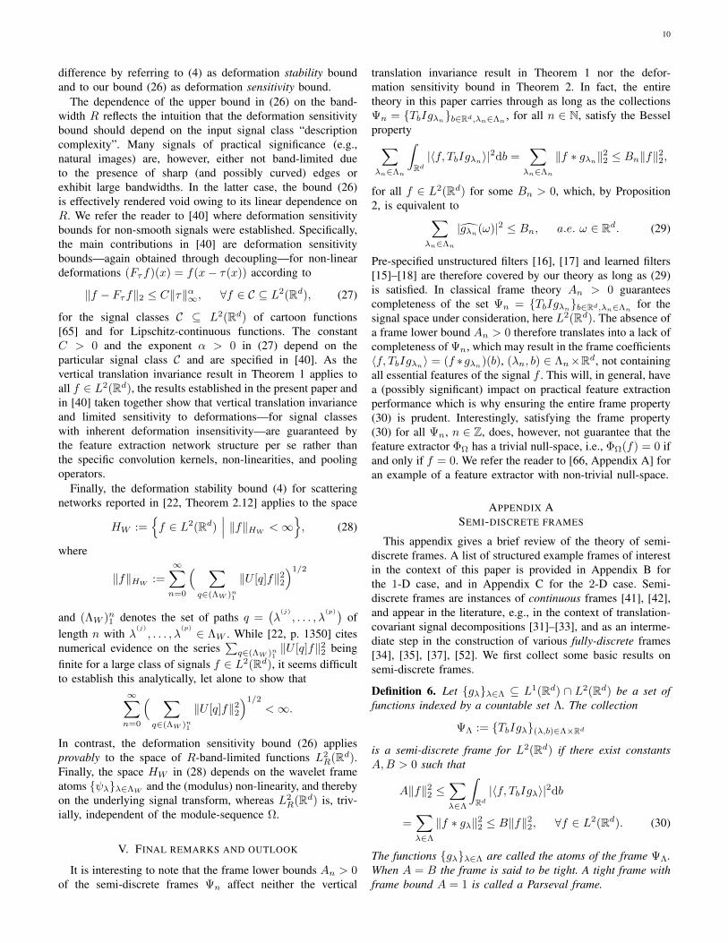
Fig. 7: Partitioning of the frequency plane R2 induced by (left) a semi-discrete tensor wavelet frame, and (right) a semi-discrete directional wavelet frame.

feature extraction tasks [55], [56]. A semi-discrete waveletframe for L2(R) is a collection of functions according to(34), where gk(x) := 2kψ(2kx), k ∈ Z, with the motherwavelet ψ ∈ L1(R) ∩ L2(R). The atoms gkk∈Z satisfy theLittlewood-Paley condition (35) according to

A ≤∑k∈Z|ψ(2−kω)|2 ≤ B, a.e. ω ∈ R. (37)

A large class of functions ψ satisfying (37) can be obtainedthrough a multi-resolution analysis in L2(R) [30, Definition7.1].

Semi-discrete curvelet frames: Curvelets, introduced in [34],[38], are well-suited to the extraction of signal featurescharacterized by curve-like singularities (such as, e.g., curvededges in images), and have been applied successfully invarious practical feature extraction tasks [60], [61].

APPENDIX CEXAMPLES OF SEMI-DISCRETE FRAMES IN 2-D

Semi-discrete wavelet frames: Two-dimensional waveletsare well-suited to the extraction of signal features characte-rized by point singularities (such as, e.g., stars in astronomicalimages [78]), and have been applied successfully in variouspractical feature extraction tasks, e.g., in [19]–[21], [32].Prominent families of two-dimensional wavelet frames aretensor wavelet frames and directional wavelet frames:

i) Semi-discrete tensor wavelet frames: A semi-discretetensor wavelet frame for L2(R2) is a collection of func-tions according to ΨΛTW := TbIg(e,j)(e,j)∈ΛTW,b∈R2 ,g(e,j)(x) := 22jψe(2jx), where ΛTW :=

((0, 0), 0)

∪

(e, j) | e ∈ E\(0, 0), j ≥ 0

, and E := 0, 12.Here, the functions ψe ∈ L1(R2) ∩ L2(R2) are tensorproducts of a coarse-scale function φ ∈ L1(R)∩L2(R)and a fine-scale function ψ ∈ L1(R)∩L2(R) accordingto ψ(0,0) := φ ⊗ φ, ψ(1,0) := ψ ⊗ φ, ψ(0,1) := φ ⊗ ψ,and ψ(1,1) := ψ ⊗ ψ. The corresponding Littlewood-Paley condition (32) reads

A ≤∣∣ψ(0,0)(ω)

∣∣2+∑j≥0

∑e∈E\(0,0)

|ψe(2−jω)|2 ≤ B, (38)

a.e. ω ∈ R2. A large class of functions φ, ψ satisfying(38) can be obtained through a multi-resolution analysisin L2(R) [30, Definition 7.1].

ii) Semi-discrete directional wavelet frames: A semi-discrete directional wavelet frame for L2(R2) is a col-lection of functions according to

ΨΛDW := TbIg(j,k)(j,k)∈ΛDW,b∈R2 ,

with g(−J,0)(x) := 2−2Jφ(2−Jx), g(j,k)(x) :=22jψ(2jRθkx), where ΛDW :=

(−J, 0)

∪

(j, k) | j ∈Z with j > −J, k ∈ 0, . . . ,K − 1

, Rθ is a 2 × 2

rotation matrix defined as

Rθ :=

(cos(θ) − sin(θ)sin(θ) cos(θ)

), θ ∈ [0, 2π), (39)

and θk := 2πkK , with k = 0, . . . ,K − 1, for a fixed

K ∈ N, are rotation angles. The functions φ ∈ L1(R2)∩L2(R2) and ψ ∈ L1(R2)∩L2(R2) are referred to in theliterature as coarse-scale wavelet and fine-scale wavelet,respectively. The integer J ∈ Z corresponds to thecoarsest scale resolved and the atoms g(j,k)(j,k)∈ΛDW

satisfy the Littlewood-Paley condition (32) according to

A ≤ |φ(2Jω)|2 +∑j>−J

K−1∑k=0

|ψ(2−jRθkω)|2 ≤ B, (40)

a.e. ω ∈ R2. Prominent examples of functions φ, ψsatisfying (40) are the Gaussian function for φ and amodulated Gaussian function for ψ [30].

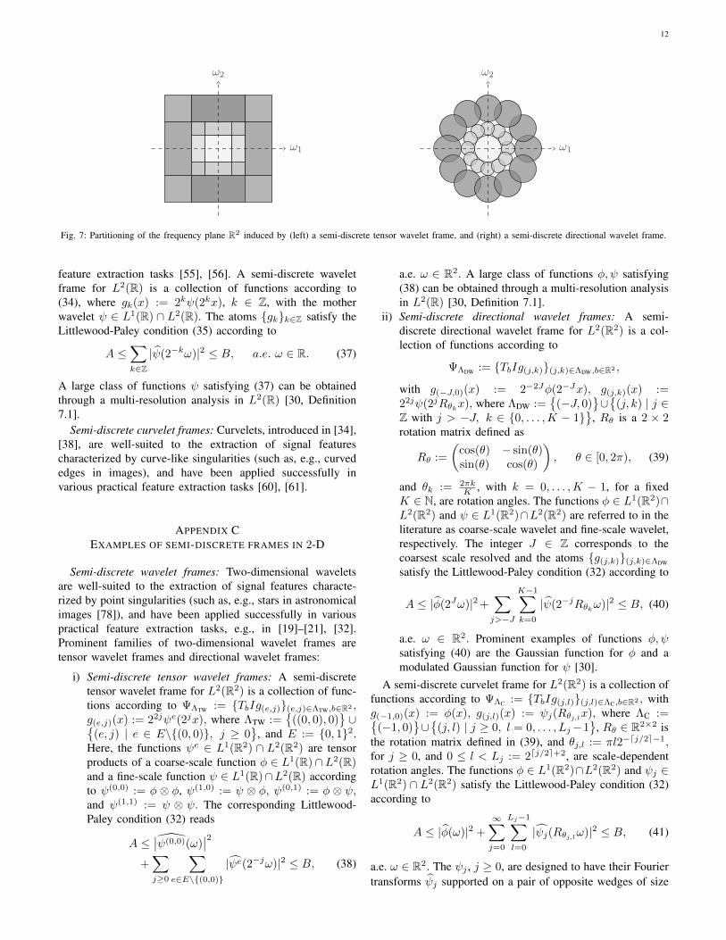
A semi-discrete curvelet frame for L2(R2) is a collection offunctions according to ΨΛC := TbIg(j,l)(j,l)∈ΛC,b∈R2 , withg(−1,0)(x) := φ(x), g(j,l)(x) := ψj(Rθj,lx), where ΛC :=

(−1, 0)∪

(j, l) | j ≥ 0, l = 0, . . . , Lj−1

, Rθ ∈ R2×2 isthe rotation matrix defined in (39), and θj,l := πl2−dj/2e−1,for j ≥ 0, and 0 ≤ l < Lj := 2dj/2e+2, are scale-dependentrotation angles. The functions φ ∈ L1(R2)∩L2(R2) and ψj ∈L1(R2) ∩ L2(R2) satisfy the Littlewood-Paley condition (32)according to

A ≤ |φ(ω)|2 +

∞∑j=0

Lj−1∑l=0

|ψj(Rθj,lω)|2 ≤ B, (41)

a.e. ω ∈ R2. The ψj , j ≥ 0, are designed to have their Fouriertransforms ψj supported on a pair of opposite wedges of size

13

ω1

ω2

ω1

ω2

Fig. 8: Partitioning of the frequency plane R2 induced by (left) a semi-discrete curvelet frame, and (right) a semi-discrete ridgelet frame.

2−j/2×2j in the dyadic corona ω ∈ R2 | 2j ≤ |ω| ≤ 2j+1,see Fig. 8 (left). We refer the reader to [34, Theorem 4.1] forconstructions of functions φ, ψj satisfying (41) with A = B =1.

Semi-discrete ridgelet frames: Ridgelets, introduced in [79],[80], are well-suited to the extraction of signal featurescharacterized by straight-line singularities (such as, e.g.,straight edges in images), and have been applied successfullyin various practical feature extraction tasks [57]–[59], [61].

A semi-discrete ridgelet frame for L2(R2) is a collectionof functions according to ΨΛR := TbIg(j,l)(j,l)∈ΛR,b∈R2 ,with g(0,0)(x) := φ(x), g(j,l)(x) := ψ(j,l)(x), where ΛR :=

(0, 0)∪

(j, l) | j ≥ 1, l = 1, . . . , 2j − 1

, and theatoms g(j,l)(j,l)∈ΛR satisfy the Littlewood-Paley condition(32) according to

A ≤ |φ(ω)|2 +

∞∑j=1

2j−1∑l=1

|ψ(j,l)(ω)|2 ≤ B, (42)

a.e. ω ∈ R2. The ψ(j,l) ∈ L1(R2) ∩ L2(R2), (j, l) ∈ΛR\(0, 0), are designed to be constant in the directionspecified by the parameter l, and to have Fourier transformsψ(j,l) supported on a pair of opposite wedges of size 2−j×2j

in the dyadic corona ω ∈ R2 | 2j ≤ |ω| ≤ 2j+1, seeFig. 8 (right). We refer the reader to [37, Proposition 6]for constructions of functions φ, ψ(j,l) satisfying (42) withA = B = 1.

Remark 3. For further examples of interesting structuredsemi-discrete frames, we refer to [36], which discusses semi-discrete shearlet frames, and [35], which deals with semi-discrete α-curvelet frames.

APPENDIX DNON-LINEARITIES

This appendix gives a brief overview of non-linearities M :L2(Rd) → L2(Rd) that are widely used in the deep learningliterature and that fit into our theory. For each example, weestablish how it satisfies the conditions on M : L2(Rd) →L2(Rd) in Theorems 1 and 2 and in Corollary 1. Specifically,we need to verify the following:(i) Lipschitz continuity: There exists a constant L ≥ 0 such

that ‖Mf −Mh‖2 ≤ L‖f − h‖2, for all f, h ∈ L2(Rd).(ii) Mf = 0 for f = 0.

All non-linearities considered here are pointwise (memoryless)operators in the sense of

M : L2(Rd)→ L2(Rd), (Mf)(x) = ρ(f(x)), (43)

where ρ : C→ C. An immediate consequence of this propertyis that the operator M commutes with the translation operatorTt (see Theorem 2 and Corollary 1):

(MTtf)(x) = ρ((Ttf)(x)) = ρ(f(x− t)) = Ttρ(f(x))

= (TtMf)(x), ∀f ∈ L2(Rd),∀t ∈ Rd.

Modulus function: The modulus function

| · | : L2(Rd)→ L2(Rd), |f |(x) := |f(x)|,

has been applied successfully in the deep learning literature,e.g., in [16], [21], and most prominently in scattering networks[22]. Lipschitz continuity with L = 1 follows from

‖|f | − |h|‖22 =

∫Rd

||f(x)| − |h(x)||2dx

≤∫Rd

|f(x)− h(x)|2dx = ‖f − h‖22,

for f, h ∈ L2(Rd), by the reverse triangle inequality. Further-more, obviously |f | = 0 for f = 0, and finally | · | is pointwiseas (43) is satisfied with ρ(x) := |x|.Rectified linear unit: The rectified linear unit non-linearity(see, e.g., [26], [27]) is defined as R : L2(Rd)→ L2(Rd),

(Rf)(x) := max0,Re(f(x))+ imax0, Im(f(x)).

We start by establishing that R is Lipschitz-continuous withL = 2. To this end, fix f, h ∈ L2(Rd). We have

|(Rf)(x)− (Rh)(x)|=∣∣max0,Re(f(x))+ imax0, Im(f(x))

−(

max0,Re(h(x))+ imax0, Im(h(x)))∣∣

≤∣∣max0,Re(f(x)) −max0,Re(h(x))

∣∣ (44)

+∣∣max0, Im(f(x)) −max0, Im(h(x))

∣∣≤∣∣Re(f(x))− Re(h(x))

∣∣+∣∣ Im(f(x))− Im(h(x))

∣∣ (45)

≤∣∣f(x)− h(x)

∣∣+∣∣f(x)− h(x)

∣∣ = 2|f(x)− h(x)|, (46)

where we used the triangle inequality in (44),

|max0, a −max0, b| ≤ |a− b|, ∀a, b ∈ R,

14

in (45), and the Lipschitz continuity (with L = 1) of themappings Re : C→ R and Im : C→ R in (46). We thereforeget

‖Rf −Rh‖2 =(∫

Rd

|(Rf)(x)− (Rh)(x)|2dx)1/2

≤ 2(∫

Rd

|f(x)− h(x)|2dx)1/2

= 2 ‖f − h‖2,

which establishes Lipschitz continuity of R with Lipschitzconstant L = 2. Furthermore, obviously Rf = 0 for f = 0,and finally (43) is satisfied with ρ(x) := max0,Re(x) +imax0, Im(x).Hyperbolic tangent: The hyperbolic tangent non-linearity (see,e.g., [15]–[17]) is defined as H : L2(Rd)→ L2(Rd),

(Hf)(x) := tanh(Re(f(x))) + i tanh(Im(f(x))),

where tanh(x) := ex−e−x

ex+e−x . We start by proving that H isLipschitz-continuous with L = 2. To this end, fix f, h ∈L2(Rd). We have

|(Hf)(x)− (Hh)(x)|=∣∣ tanh(Re(f(x))) + i tanh(Im(f(x)))

−(

tanh(Re(h(x))) + i tanh(Im(h(x))))∣∣

≤∣∣ tanh(Re(f(x)))− tanh(Re(h(x)))

∣∣+∣∣ tanh(Im(f(x)))− tanh(Im(h(x)))

∣∣, (47)

where, again, we used the triangle inequality. In order tofurther upper-bound (47), we show that tanh is Lipschitz-continuous. To this end, we make use of the following result.

Lemma 1. Let h : R → R be a continuously differentiablefunction satisfying supx∈R |h′(x)| ≤ L. Then, h is Lipschitz-continuous with Lipschitz constant L.

Proof. See [81, Theorem 9.5.1].

Since tanh′(x) = 1 − tanh2(x), x ∈ R, we havesupx∈R | tanh′(x)| ≤ 1. By Lemma 1 we can thereforeconclude that tanh is Lipschitz-continuous with L = 1, whichwhen used in (47), yields

|(Hf)(x)− (Hh)(x)| ≤∣∣Re(f(x))− Re(h(x))

∣∣+∣∣ Im(f(x))− Im(h(x))

∣∣≤∣∣f(x)− h(x)

∣∣+∣∣f(x)− h(x)

∣∣= 2|f(x)− h(x)|.

Here, again, we used the Lipschitz continuity (with L = 1) ofRe : C → R and Im : C → R. Putting things together, weobtain

‖Hf −Hh‖2 =(∫

Rd

|(Hf)(x)− (Hh)(x)|2dx)1/2

≤ 2(∫

Rd

|f(x)− h(x)|2dx)1/2

= 2 ‖f − h‖2,

which proves that H is Lipschitz-continuous with L = 2.Since tanh(0) = 0, we trivially have Hf = 0 for f =

0. Finally, (43) is satisfied with ρ(x) := tanh(Re(x)) +i tanh(Im(x)).

Shifted logistic sigmoid: The shifted logistic sigmoid non-linearity10 (see, e.g., [28], [29]) is defined as P : L2(Rd) →L2(Rd),

(Pf)(x) := sig(Re(f(x))) + isig(Im(f(x))),

where sig(x) := 11+e−x − 1

2 . We first establish that P isLipschitz-continuous with L = 1

2 . To this end, fix f, h ∈L2(Rd). We have

|(Pf)(x)− (Ph)(x)| =∣∣sig(Re(f(x))) + isig(Im(f(x)))

−(sig(Re(h(x))) + isig(Im(h(x)))

)∣∣≤∣∣sig(Re(f(x)))− sig(Re(h(x)))

∣∣+∣∣sig(Im(f(x)))− sig(Im(h(x)))

∣∣, (48)

where, again, we employed the triangle inequality. As before,to further upper-bound (48), we show that sig is Lipschitz-continuous. Specifically, we apply Lemma 1 with sig′(x) =

e−x

(1+e−x)2 , x ∈ R, and hence supx∈R |sig′(x)| ≤ 14 , to conclude

that sig is Lipschitz-continuous with L = 14 . When used in

(48) this yields (together with the Lipschitz continuity, withL = 1, of Re : C→ R and Im : C→ R)

|(Pf)(x)− (Ph)(x)| ≤ 1

4

∣∣∣Re(f(x))− Re(h(x))∣∣∣

+1

4

∣∣∣ Im(f(x))− Im(h(x))∣∣∣ ≤ 1

4

∣∣∣f(x)− h(x)∣∣∣

+1

4

∣∣∣f(x)− h(x)∣∣∣ =

1

2

∣∣∣f(x)− h(x)∣∣∣. (49)

It now follows from (49) that

‖Pf − Ph‖2 =(∫

Rd

|(Pf)(x)− (Ph)(x)|2dx)1/2

≤1

2

(∫Rd

|f(x)− h(x)|2dx)1/2

=1

2‖f − h‖2,

which establishes Lipschitz continuity of P with L = 12 . Since

sig(0) = 0, we trivially have Pf = 0 for f = 0. Finally, (43)is satisfied with ρ(x) := sig(Re(x)) + isig(Im(x)).

APPENDIX EPROOF OF PROPOSITION 1

We need to show that ΦΩ(f) ∈ (L2(Rd))Q, for allf ∈ L2(Rd). This will be accomplished by proving an evenstronger result, namely

|||ΦΩ(f)||| ≤ ‖f‖2, ∀f ∈ L2(Rd), (50)

which, by ‖f‖2 < ∞, establishes the claim. For ease ofnotation, we let fq := U [q]f , for f ∈ L2(Rd), in the following.Thanks to (14) and (17), we have ‖fq‖2 ≤ ‖f‖2 < ∞, andthus fq ∈ L2(Rd). The key idea of the proof is now—similarly

10Strictly speaking, it is actually the sigmoid function x 7→ 11+e−x rather

than the shifted sigmoid function x 7→ 11+e−x − 1

2that is used in [28], [29].

We incorporated the offset 12

in order to satisfy the requirement Pf = 0 forf = 0.

15

to the proof of [22, Proposition 2.5]—to judiciously employ atelescoping series argument. We start by writing

|||ΦΩ(f)|||2 =

∞∑n=0

∑q∈Λn

1

||fq ∗ χn||22

= limN→∞

N∑n=0

∑q∈Λn

1

||fq ∗ χn||22︸ ︷︷ ︸:=an

. (51)

The key step is then to establish that an can be upper-boundedaccording to

an ≤ bn − bn+1, ∀n ∈ N0, (52)

with bn :=∑q∈Λn

1‖fq‖22, n ∈ N0, and to use this result in a

telescoping series argument according toN∑n=0

an ≤N∑n=0

(bn − bn+1) = (b0 − b1) + (b1 − b2)

+ · · ·+ (bN − bN+1) = b0 − bN+1︸ ︷︷ ︸≥0

(53)

≤ b0 =∑q∈Λ0

1

‖fq‖22 = ‖U [e]f‖22 = ‖f‖22. (54)

By (51) this then implies (50). We start by noting that (52)reads ∑

q∈Λn1

‖fq ∗ χn‖22 ≤∑q∈Λn

1

||fq‖22 −∑

q∈Λn+11

‖fq‖22, (55)

for all n ∈ N0, and proceed by examining the second term onthe right hand side (RHS) of (55). Every path

q ∈ Λn+11 = Λ1 × · · · × Λn︸ ︷︷ ︸

=Λn1

×Λn+1

of length n+1 can be decomposed into a path q ∈ Λn1 of lengthn and an index λn+1 ∈ Λn+1 according to q = (q, λn+1).Thanks to (13) we have

U [q] = U [(q, λn+1)] = Un+1[λn+1]U [q],

which yields∑q∈Λn+1

1

‖fq‖22 =∑q∈Λn

1

∑λn+1∈Λn+1

‖Un+1[λn+1]fq‖22. (56)

Substituting the second term on the RHS of (55) by (56) nowyields∑q∈Λn

1

‖fq ∗ χn‖22

≤∑q∈Λn

1

(||fq‖22 −

∑λn+1∈Λn+1

‖Un+1[λn+1]fq‖22), ∀n ∈ N0,

which can be rewritten as∑q∈Λn

1

(‖fq ∗ χn‖22 +

∑λn+1∈Λn+1

‖Un+1[λn+1]fq‖22)

(57)

≤∑q∈Λn

1

||fq‖22, ∀n ∈ N0.

Next, note that the second term inside the sum on the left handside (LHS) of (57) can be written as∑λn+1∈Λn+1

‖Un+1[λn+1]fq‖22

=∑

λn+1∈Λn+1

∫Rd

|(Un+1[λn+1]fq)(x)|2dx

=∑

λn+1∈Λn+1

Sdn+1

∫Rd

∣∣∣Pn+1

(Mn+1(fq ∗ gλn+1

))(Sn+1x)

∣∣∣2dx

=∑

λn+1∈Λn+1

∫Rd

∣∣∣Pn+1

(Mn+1(fq ∗ gλn+1

))(y)∣∣∣2dy

=∑

λn+1∈Λn+1

‖Pn+1

(Mn+1(fq ∗ gλn+1

))‖22, (58)

for all n ∈ N0. Noting that fq ∈ L2(Rd), as established above,and gλn+1

∈ L1(Rd), by assumption, it follows that (fq ∗gλn+1

) ∈ L2(Rd) thanks to Young’s inequality [63, Theorem1.2.12]. We use the Lipschitz property of Mn+1 and Pn+1,i.e., ‖Mn+1(fq ∗gλn+1)−Mn+1h‖2 ≤ Ln+1‖fq ∗gλn+1−h‖,and ‖Pn+1(fq ∗ gλn+1

)− Pn+1h‖2 ≤ Rn+1‖fq ∗ gλn+1− h‖,

together with Mn+1h = 0 and Pn+1h = 0 for h = 0, toupper-bound the term inside the sum in (58) according to

‖Pn+1

(Mn+1(fq ∗ gλn+1

))‖22 ≤ R2

n+1‖Mn+1(fq ∗ gλn+1)‖22

≤ L2n+1R

2n+1‖fq ∗ gλn+1

‖22, ∀n ∈ N0. (59)

Substituting the second term inside the sum on the LHS of(57) by the upper bound resulting from insertion of (59) into(58) yields∑

q∈Λn1

(‖fq ∗ χn‖22 + L2

n+1R2n+1

∑λn+1∈Λn+1

‖fq ∗ gλn+1‖22)

≤∑q∈Λn

1

max1, L2n+1R

2n+1

(‖fq ∗ χn‖22

+∑

λn+1∈Λn+1

‖fq ∗ gλn+1‖22), ∀n ∈ N0. (60)

As the functions gλn+1λn+1∈Λn+1 ∪ χn are the atoms ofthe semi-discrete frame Ψn+1 for L2(Rd) and fq ∈ L2(Rd),as established above, we have

‖fq ∗ χn‖22 +∑

λn+1∈Λn+1

‖fq ∗ gλn+1‖22 ≤ Bn+1‖fq‖22,

which, when used in (60) yields∑q∈Λn

1

(‖fq ∗ χn‖22 +

∑λn+1∈Λn+1

‖Un+1[λn+1]fq‖22)

≤∑q∈Λn

1

max1, L2n+1R

2n+1Bn+1‖fq‖22

=∑q∈Λn

1

maxBn+1, Bn+1L2n+1R

2n+1‖fq‖22, (61)

for all n ∈ N0. Finally, invoking the assumption

maxBn, BnL2nR

2n+1 ≤ 1, ∀n ∈ N,

in (61) yields (57) and thereby completes the proof.

16

APPENDIX FPROOF OF THEOREM 1

We start by proving i). The key step in establishing (19) isto show that the operator Un, n ∈ N, defined in (10) satisfiesthe relation

Un[λn]Ttf = Tt/SnUn[λn]f, (62)

for all f ∈ L2(Rd), t ∈ Rd, and λn ∈ Λn. With the definitionof U [q] in (13) this then yields

U [q]Ttf = Tt/(S1···Sn)U [q]f, (63)

for all f ∈ L2(Rd), t ∈ Rd, and q ∈ Λn1 . The identity(19) is then a direct consequence of (63) and the translation-covariance of the convolution operator:

ΦnΩ(Ttf) =(U [q]Ttf

)∗ χn

q∈Λn

1

=(Tt/(S1···Sn)U [q]f

)∗ χn

q∈Λn

1

=Tt/(S1···Sn)

((U [q]f) ∗ χn

)q∈Λn

1

= Tt/(S1···Sn)

(U [q]f) ∗ χn

q∈Λn

1

= Tt/(S1···Sn)ΦnΩ(f), ∀f ∈ L2(Rd), ∀t ∈ Rd.

To establish (62), we first define the unitary operator

Dn : L2(Rd)→ L2(Rd), Dnf := Sd/2n f(Sn·),

and note that

Un[λn]Ttf = Sd/2n Pn

(Mn

((Ttf) ∗ gλn

))(Sn·)

= DnPn

(Mn

((Ttf) ∗ gλn

))= DnPn

(Mn

(Tt(f ∗ gλn

)))

= DnPn

(Tt(Mn(f ∗ gλn

)))

(64)

= DnTt

(Pn

((Mn(f ∗ gλn)

))), (65)

for all f ∈ L2(Rd) and t ∈ Rd, where in (64) and (65) weemployed

MnTt = TtMn, and PnTt = TtPn,

for all n ∈ N and t ∈ Rd, respectively, both of which are byassumption. Next, using

DnTtf = Sd/2n f(Sn · −t) = Sd/2n f(Sn(· − t/Sn))

= Tt/SnDnf, ∀f ∈ L2(Rd), ∀t ∈ Rd,

in (65) yields

Un[λn]Ttf = DnTt

(Pn

((Mn(f ∗ gλn)

)))= Tt/Sn

(DnPn

((Mn(f ∗ gλn

))))

= Tt/SnUn[λn]f,

for all f ∈ L2(Rd) and t ∈ Rd. This completes the proof ofi).

Next, we prove ii). For ease of notation, again, we let fq :=U [q]f , for f ∈ L2(Rd). Thanks to (14) and the admissibility

condition (17), we have ‖fq‖2 ≤ ‖f‖2 < ∞, and thus fq ∈L2(Rd). We first write

|||ΦnΩ(Ttf)− ΦnΩ(f)|||2

= |||Tt/(S1···Sn)ΦnΩ(f)− ΦnΩ(f)|||2 (66)

=∑q∈Λn

1

‖Tt/(S1···Sn)(fq ∗ χn)− fq ∗ χn‖22

=∑q∈Λn

1

‖M−t/(S1···Sn)(fq ∗ χn)− fq ∗ χn‖22, (67)

for all n ∈ N, where in (66) we used (19), and in (67) weemployed Parseval’s formula [43, p. 189] (noting that (fq ∗χn) ∈ L2(Rd) thanks to Young’s inequality [63, Theorem1.2.12]) together with the relation

Ttf = M−tf , ∀f ∈ L2(Rd),∀ t ∈ Rd.

The key step is then to establish the upper bound

‖M−t/(S1···Sn)(fq ∗ χn)− fq ∗ χn‖22

≤ 4π2|t|2K2

(S1 · · ·Sn)2‖fq‖22, ∀n ∈ N, (68)

where K > 0 corresponds to the constant in the decaycondition (20), and to note that∑

q∈Λn1

‖fq‖22 ≤∑

q∈Λn−11

‖fq‖22, ∀n ∈ N, (69)

which follows from (52) thanks to

0 ≤∑

q∈Λn−11

||fq ∗ χn−1||22 = an−1 ≤ bn−1 − bn (70)

=∑

q∈Λn−11

‖fq‖22 −∑q∈Λn

1

‖fq‖22, ∀n ∈ N. (71)

Iterating on (69) yields∑q∈Λn

1

‖fq‖22 ≤∑

q∈Λn−11

‖fq‖22 ≤ · · · ≤∑q∈Λ0

1

‖fq‖22

= ‖U [e]f‖22 = ‖f‖22, ∀n ∈ N. (72)

The identity (67) together with the inequalities (68) and (72)then directly imply

|||ΦnΩ(Ttf)− ΦnΩ(f)|||2 ≤ 4π2|t|2K2

(S1 · · ·Sn)2‖f‖22, (73)

for all n ∈ N. It remains to prove (68). To this end, we firstnote that

‖M−t/(S1···Sn)(fq ∗ χn)− fq ∗ χn‖22

=

∫Rd

∣∣e−2πi〈t,ω〉/(S1···Sn) − 1∣∣2|χn(ω)|2|fq(ω)|2dω. (74)

Since |e−2πix − 1| ≤ 2π|x|, for all x ∈ R, it follows that

|e−2πi〈t,ω〉/(S1···Sn) − 1|2 ≤ 4π2|〈t, ω〉|2

(S1 · · ·Sn)2

≤ 4π2|t|2|ω|2

(S1 · · ·Sn)2, (75)

where in the last step we employed the Cauchy-Schwartz

17

inequality. Substituting (75) into (74) yields

‖M−t/(S1···Sn)(fq ∗ χn)− fq ∗ χn‖22

≤ 4π2|t|2

(S1 · · ·Sn)2

∫Rd

|ω|2|χn(ω)|2|fq(ω)|2dω

≤ 4π2|t|2K2

(S1 · · ·Sn)2

∫Rd

|fq(ω)|2dω (76)

=4π2|t|2K2

(S1 · · ·Sn)2‖fq‖22 =

4π2|t|2K2

(S1 · · ·Sn)2‖fq‖22, (77)

for all n ∈ N, where in (76) we employed the decay condition(20), and in the last step, again, we used Parseval’s formula[43, p. 189]. This establishes (68) and thereby completes theproof of ii).

APPENDIX GPROOF OF COROLLARY 1

The key idea of the proof is—similarly to the proof ofii) in Theorem 1—to upper-bound the deviation from perfectcovariance in the frequency domain. For ease of notation,again, we let fq := U [q]f , for f ∈ L2(Rd). Thanks to (14) andthe admissibility condition (17), we have ‖fq‖2 ≤ ‖f‖2 <∞,and thus fq ∈ L2(Rd). We first write

|||ΦnΩ(Ttf)− TtΦnΩ(f)|||2

= |||Tt/(S1···Sn)ΦnΩ(f)− TtΦnΩ(f)|||2 (78)

=∑q∈Λn

1

‖(Tt/(S1···Sn) − Tt)(fq ∗ χn)‖22

=∑q∈Λn

1

‖(M−t/(S1···Sn) −M−t)(fq ∗ χn)‖22, (79)

for all n ∈ N, where in (78) we used (19), and in (79) weemployed Parseval’s formula [43, p. 189] (noting that (fq ∗χn) ∈ L2(Rd) thanks to Young’s inequality [63, Theorem1.2.12]) together with the relation

Ttf = M−tf , ∀f ∈ L2(Rd),∀ t ∈ Rd.

The key step is then to establish the upper bound

‖(M−t/(S1···Sn) −M−t)(fq ∗ χn)‖22≤ 4π2|t|2K2

∣∣1/(S1 · · ·Sn)− 1∣∣2‖fq‖22, (80)

where K > 0 corresponds to the constant in the decaycondition (20). Arguments similar to those leading to (73) thencomplete the proof. It remains to prove (80):

‖(M−t/(S1···Sn) −M−t)(fq ∗ χn)‖22

=

∫Rd

∣∣e−2πi〈t,ω〉/(S1···Sn)

− e−2πi〈t,ω〉∣∣2|χn(ω)|2|fq(ω)|2dω. (81)

Since |e−2πix − e−2πiy| ≤ 2π|x − y|, for all x, y ∈ R, itfollows that ∣∣e−2πi〈t,ω〉/(S1···Sn) − e−2πi〈t,ω〉∣∣2

≤ 4π2|t|2|ω|2∣∣1/(S1 · · ·Sn)− 1

∣∣2, (82)

where, again, we employed the Cauchy-Schwartz inequality.Substituting (82) into (81), and employing arguments similar

to those leading to (77), establishes (80) and thereby completesthe proof.

APPENDIX HPROOF OF THEOREM 2

As already mentioned at the beginning of Section IV-B,the proof of the deformation sensitivity bound (26) is basedon two key ingredients. The first one, stated in Proposition4 in Appendix I, establishes that the feature extractor ΦΩ isLipschitz-continuous with Lipschitz constant LΩ = 1, i.e.,

|||ΦΩ(f)− ΦΩ(h)||| ≤ ‖f − h‖2, ∀f, h ∈ L2(Rd), (83)

and needs the admissibility condition (17) only. The secondingredient, stated in Proposition 5 in Appendix J, is an upperbound on the deformation error ‖f − Fτ,ωf‖2 given by

‖f − Fτ,ωf‖2 ≤ C(R‖τ‖∞ + ‖ω‖∞

)‖f‖2, (84)

for all f ∈ L2R(Rd), and is valid under the assumptions ω ∈

C(Rd,R) and τ ∈ C1(Rd,Rd) with ‖Dτ‖∞ < 12d . We now

show how (83) and (84) can be combined to establish thedeformation sensitivity bound (26). To this end, we first apply(83) with h := Fτ,ωf = e2πiω(·)f(· − τ(·)) to get

|||ΦΩ(f)− ΦΩ(Fτ,ωf)||| ≤ ‖f − Fτ,ωf‖2, (85)

for all f ∈ L2(Rd). Here, we used Fτ,ωf ∈ L2(Rd), which isthanks to

‖Fτ,ωf‖22 =

∫Rd

|f(x− τ(x))|2dx ≤ 2‖f‖22,

obtained through the change of variables u = x − τ(x),together with

du

dx= |det(E − (Dτ)(x))| ≥ 1− d‖Dτ‖∞ ≥ 1/2, (86)

for x ∈ Rd. The first inequality in (86) follows from:

Lemma 2. [82, Corollary 1]: Let M ∈ Rd×d be such that|Mi,j | ≤ α, for all i, j with 1 ≤ i, j ≤ d. If dα ≤ 1, then

|det(E −M)| ≥ 1− dα.

The second inequality in (86) is a consequence of theassumption ‖Dτ‖∞ ≤ 1

2d . The proof is finalized by replacingthe RHS of (85) by the RHS of (84).

APPENDIX IPROPOSITION 4

Proposition 4. Let Ω =((Ψn,Mn, Pn)

)n∈N be an admissible

module-sequence. The corresponding feature extractor ΦΩ :L2(Rd) → (L2(Rd))Q is Lipschitz-continuous with Lipschitzconstant LΩ = 1, i.e.,

|||ΦΩ(f)− ΦΩ(h)||| ≤ ‖f − h‖2, ∀f, h ∈ L2(Rd). (87)

Remark 4. Proposition 4 generalizes [22, Proposition 2.5],which shows that the wavelet-modulus feature extractor ΦWgenerated by scattering networks is Lipschitz-continuous withLipschitz constant LW = 1. Specifically, our generalizationallows for general semi-discrete frames (i.e., general convolu-tion kernels), general Lipschitz-continuous non-linearities Mn,

18

and general Lipschitz-continuous operators Pn, all of whichcan be different in different layers. Moreover, thanks to theadmissibility condition (17), the Lipschitz constant LΩ = 1in (87) is completely independent of the frame upper boundsBn and the Lipschitz-constants Ln and Rn of Mn and Pn,respectively.

Proof. The key idea of the proof is again—similarly to theproof of Proposition 1 in Appendix E—to judiciously employ atelescoping series argument. For ease of notation, we let fq :=U [q]f and hq := U [q]h, for f, h ∈ L2(Rd). Thanks to (14) andthe admissibility condition (17), we have ‖fq‖2 ≤ ‖f‖2 <∞and ‖hq‖2 ≤ ‖h‖2 < ∞ and thus fq, hq ∈ L2(Rd). We startby writing

|||ΦΩ(f)− ΦΩ(h)|||2 =

∞∑n=0

∑q∈Λn

1

||fq ∗ χn − hq ∗ χn||22

= limN→∞

N∑n=0

∑q∈Λn

1

||fq ∗ χn − hq ∗ χn||22︸ ︷︷ ︸=:an

.

As in the proof of Proposition 1 in Appendix E, the key stepis to show that an can be upper-bounded according to

an ≤ bn − bn+1, ∀n ∈ N0, (88)

where here

bn :=∑q∈Λn

1

‖fq − hq‖22, ∀n ∈ N0,

and to note that, similarly to (54),N∑n=0

an ≤N∑n=0

(bn − bn+1) = (b0 − b1) + (b1 − b2)

+ · · ·+ (bN − bN+1) = b0 − bN+1︸ ︷︷ ︸≥0

≤ b0 =∑q∈Λ0

1

‖fq − hq‖22 = ‖U [e]f − U [e]h‖22

= ‖f − h‖22,

which then yields (87) according to

|||ΦΩ(f)− ΦΩ(h)|||2 = limN→∞

N∑n=0

an ≤ limN→∞

‖f − h‖22

= ‖f − h‖22.

Writing out (88), it follows that we need to establish∑q∈Λn

1

‖fq ∗ χn − hq ∗ χn‖22

≤∑q∈Λn

1

||fq − hq‖22 −∑

q∈Λn+11

‖fq − hq‖22, (89)

for all n ∈ N0. We start by examining the second term on theRHS of (89) and note that, thanks to the decomposition

q ∈ Λn+11 = Λ1 × · · · × Λn︸ ︷︷ ︸

=Λn1

×Λn+1

and U [q] = U [(q, λn+1)] = Un+1[λn+1]U [q], by (13), wehave ∑

q∈Λn+11

‖fq − hq‖22 =∑q∈Λn

1

∑λn+1∈Λn+1

‖Un+1[λn+1]fq

− Un+1[λn+1]hq‖22. (90)

Substituting (90) into (89) and rearranging terms, we obtain∑q∈Λn

1

(‖fq ∗ χn − hq ∗ χn‖22

+∑

λn+1∈Λn+1

‖Un+1[λn+1]fq − Un+1[λn+1]hq‖22)

≤∑q∈Λn

1

||fq − hq‖22, ∀n ∈ N0. (91)

We next note that the second term inside the sum on the LHSof (91) satisfies∑

λn+1∈Λn+1

‖Un+1[λn+1]fq − Un+1[λn+1]hq‖22

≤∑

λn+1∈Λn+1

‖Pn+1

(Mn+1(fq ∗ gλn+1

))

− Pn+1

(Mn+1(hq ∗ gλn+1

))‖22, (92)

where we employed arguments similar to those leading to (58).Substituting the second term inside the sum on the LHS of (91)by the upper bound (92), and using the Lipschitz property ofMn+1 and Pn+1 yields∑

q∈Λn1

(‖fq ∗ χn − hq ∗ χn‖22

+∑

λn+1∈Λn+1

‖Un+1[λn+1]fq − Un+1[λn+1]hq‖22)

≤∑q∈Λn

1

max1, L2n+1R

2n+1

(‖(fq − hq) ∗ χn‖22

+∑

λn+1∈Λn+1

‖(fq − hq) ∗ gλn+1‖22), (93)

for all n ∈ N0. As the functions gλn+1λn+1∈Λn+1

∪ χnare the atoms of the semi-discrete frame Ψn+1 for L2(Rd)and fq, hq ∈ L2(Rd), as established above, we have

‖(fq − hq) ∗ χn‖22 +∑

λn+1∈Λn+1

‖(fq − hq) ∗ gλn+1‖22

≤ Bn+1‖fq − hq‖22,

which, when used in (93) yields∑q∈Λn

1

(‖fq ∗ χn − hq ∗ χn‖22

+∑

λn+1∈Λn+1

‖Un+1[λn+1]fq − Un+1[λn+1]hq‖22)

≤∑q∈Λn

1

maxBn+1, Bn+1L2n+1R

2n+1‖fq − hq‖22, (94)

for all n ∈ N0. Finally, invoking the admissibility condition

maxBn, BnL2nR

2n ≤ 1, ∀n ∈ N,

19

in (94) we get (91) and hence (88). This completes the proof.

APPENDIX JPROPOSITION 5

Proposition 5. There exists a constant C > 0 such that forall f ∈ L2

R(Rd), ω ∈ C(Rd,R), and τ ∈ C1(Rd,Rd) with‖Dτ‖∞ < 1

2d , it holds that

‖f − Fτ,ωf‖2 ≤ C(R‖τ‖∞ + ‖ω‖∞

)‖f‖2. (95)

Remark 5. A similar bound was derived in [22, App. B] forscattering networks, namely

‖f ∗ψ(−J,0)−Fτ (f ∗ψ(−J,0))‖2 ≤ C2−J+d‖τ‖∞‖f‖2, (96)

for all f ∈ L2(Rd), where ψ(−J,0) is the low-pass filter ofa semi-discrete directional wavelet frame for L2(Rd), and(Fτf)(x) = f(x − τ(x)). The techniques for proving (95)and (96) are related in the sense of both employing Schur’sLemma [63, App. I.1] and a Taylor series expansion argument[83, p. 411]. The signal-class specificity of our bound (95)comes with new technical elements detailed at the beginningof the proof.

Proof. We first determine an integral operator

(Kf)(x) =

∫Rd

k(x, u)f(u)du (97)

satisfying the signal-class specific identity

Kf = Fτ,ωf − f, ∀f ∈ L2(Rd),

and then upper-bound the deformation error ‖f − Fτ,ωf‖2according to

‖f − Fτ,ωf‖2 = ‖Fτ,ωf − f‖2 = ‖Kf‖2 ≤ ‖K‖2,2‖f‖2,

for all f ∈ L2R(Rd). Application of Schur’s Lemma, stated

below, then yields

‖K‖2,2 ≤ C(R‖τ‖∞ + ‖ω‖∞

), with C > 0,

which completes the proof.

Schur’s Lemma. [63, App. I.1]: Let k : Rd ×Rd → C be alocally integrable function satisfying

(i) supx∈Rd

∫Rd

|k(x, u)|du ≤ α,

(ii) supu∈Rd

∫Rd

|k(x, u)|dx ≤ α, (98)

where α > 0. Then, (Kf)(x) =∫Rd k(x, u)f(u)du is a

bounded operator from L2(Rd) to L2(Rd) with operator norm‖K‖2,2 ≤ α.

We start by determining the integral operator K in (97). Tothis end, consider η ∈ S(Rd,C) such that η(ω) = 1, for allω ∈ B1(0). Setting γ(x) := Rdη(Rx) yields γ ∈ S(Rd,C)and γ(ω) = η(ω/R). Thus, γ(ω) = 1, for all ω ∈ BR(0), andhence f = f ·γ, so that f = f∗γ, for all f ∈ L2

R(Rd). Next, wedefine the operator Aγ : L2(Rd)→ L2(Rd), Aγf := f∗γ, andnote that Aγ is well-defined, i.e., Aγf ∈ L2(Rd), for all f ∈

L2(Rd), thanks to Young’s inequality [63, Theorem 1.2.12](since f ∈ L2(Rd) and γ ∈ S(Rd,C) ⊆ L1(Rd)). Moreover,Aγf = f , for all f ∈ L2

R(Rd). Setting K := Fτ,ωAγ−Aγ , weget Kf = Fτ,ωAγf −Aγf = Fτ,ωf −f , for all f ∈ L2

R(Rd),as desired. Furthermore, it follows from

(Fτ,ωAγf)(x) = e2πiω(x)

∫Rd

γ(x− τ(x)− u)f(u)du,

that the integral operator K = Fτ,ωAγ −Aγ , i.e.,

(Kf)(x) =

∫Rd

k(x, u)f(u)du,

has the kernel

k(x, u) := e2πiω(x)γ(x− τ(x)− u)− γ(x− u). (99)

Before we can apply Schur’s Lemma to establish an upperbound on ‖K‖2,2, we need to verify that k in (99) is locallyintegrable, i.e., we need to show that for every compact setS ⊆ Rd × Rd we have∫

S

|k(x, u)|d(x, u) <∞.

To this end, let S ⊆ Rd ×Rd be a compact set. Next, choosecompact sets S1, S2 ⊆ Rd such that S ⊆ S1 × S2. Thanksto γ ∈ S(Rd,C), τ ∈ C1(Rd,Rd), and ω ∈ C(Rd,R), allby assumption, the function |k| : S1 × S2 → C is continuousas a composition of continuous functions, and therefore alsoLebesgue-measurable. We further have∫

S1

∫S2

|k(x, u)|dxdu ≤∫S1

∫Rd

|k(x, u)|dxdu

≤∫S1

∫Rd

|γ(x− τ(x)− u)|dxdu+

∫S1

∫Rd

|γ(x− u)|dxdu

≤ 2

∫S1

∫Rd

|γ(y)|dydu+

∫S1

∫Rd

|γ(y)|dy du (100)

= 3µL(S1)‖γ‖1 <∞,

where the first term in (100) follows by the change of variablesy = x− τ(x)− u, together with

dy

dx= |det(E − (Dτ)(x))| ≥ 1− d‖Dτ‖∞ ≥ 1/2, (101)

for all x ∈ Rd. The arguments underlying (101) were alreadydetailed at the end of Appendix H. It follows that k is locallyintegrable owing to∫

S

|k(x, u)|d(x, u) ≤∫S1×S2

|k(x, u)|d(x, u)

=

∫S1

∫S2

|k(x, u)|dxdu <∞, (102)

where the first step in (102) follows from S ⊆ S1 × S2,the second step is thanks to the Fubini-Tonelli Theorem [84,Theorem 14.2] noting that |k| : S1 × S2 → C is Lebesgue-measurable (as established above) and non-negative, and thelast step is due to (100). Next, we need to verify conditions(i) and (ii) in (98) and determine the corresponding α > 0. Infact, we seek a specific constant α of the form

α = C(R‖τ‖∞ + ‖ω‖∞

), with C > 0. (103)

20

This will be accomplished as follows: For x, u ∈ Rd, weparametrize the integral kernel in (99) according to hx,u(t) :=e2πitω(x)γ(x−tτ(x)−u)−γ(x−u). A Taylor series expansion[83, p. 411] of hx,u(t) w.r.t. the variable t now yields

hx,u(t) = hx,u(0)︸ ︷︷ ︸=0

+

∫ t

0

h′x,u(λ)dλ =

∫ t

0

h′x,u(λ)dλ, (104)

for t ∈ R, where h′x,u(t) = ( ddthx,u)(t). Note that hx,u ∈

C1(R,C) thanks to γ ∈ S(Rd,C). Setting t = 1 in (104) weget

|k(x, u)| = |hx,u(1)| ≤∫ 1

0

|h′x,u(λ)|dλ, (105)

where

h′x,u(λ) = −e2πiλω(x)〈∇γ(x− λτ(x)− u), τ(x)〉+ 2πiω(x)e2πiλω(x)γ(x− λτ(x)− u), (106)

for λ ∈ [0, 1]. We further have

|h′x,u(λ)| ≤∣∣⟨∇γ(x− λτ(x)− u), τ(x)

⟩∣∣+ |2πω(x)γ(x− λτ(x)− u)|≤ |τ(x)||∇γ(x− λτ(x)− u)|+ 2π|ω(x)||γ(x− λτ(x)− u)|. (107)

Now, using |τ(x)| ≤ supy∈Rd |τ(y)| = ‖τ‖∞ and |ω(x)| ≤supy∈Rd |ω(y)| = ‖ω‖∞ in (107), together with (105), we getthe upper bound

|k(x, u)| ≤ ‖τ‖∞∫ 1

0

|∇γ(x− λτ(x)− u)|dλ

+ 2π‖ω‖∞∫ 1

0

|γ(x− λτ(x)− u)|dλ. (108)

Next, we integrate (108) w.r.t. u to establish (i) in (98):∫Rd

|k(x, u)|du

≤‖τ‖∞∫Rd

∫ 1

0

|∇γ(x− λτ(x)− u)|dλdu

+ 2π‖ω‖∞∫Rd

∫ 1

0

|γ(x− λτ(x)− u)|dλdu

= ‖τ‖∞∫ 1

0

∫Rd

|∇γ(x− λτ(x)− u)|dudλ

+ 2π‖ω‖∞∫ 1

0

∫Rd

|γ(x− λτ(x)− u)|dudλ (109)

= ‖τ‖∞∫ 1

0

∫Rd

|∇γ(y)|dydλ

+ 2π‖ω‖∞∫ 1

0

∫Rd

|γ(y)|dydλ

= ‖τ‖∞‖∇γ‖1 + 2π‖ω‖∞‖γ‖1, (110)

where (109) follows by application of the Fubini-Tonelli The-orem [84, Theorem 14.2] noting that the functions (u, λ) 7→|∇γ(x−λτ(x)−u)|, (u, λ) ∈ Rd×[0, 1], and (u, λ) 7→ |γ(x−λτ(x) − u)|, (u, λ) ∈ Rd × [0, 1], are both non-negative andcontinuous (and thus Lebesgue-measurable) as compositionsof continuous functions. Finally, using γ = Rdη(R·), and thus

∇γ = Rd+1∇η(R·), ‖γ‖1 = ‖η‖1, and ‖∇γ‖1 = R‖∇η‖1 in(110) yields

supx∈Rd

∫Rd

|k(x, u)|du ≤ R‖τ‖∞‖∇η‖1 + 2π‖ω‖∞‖η‖1

≤ max‖∇η‖1, 2π‖η‖1

(R‖τ‖∞ + ‖ω‖∞

), (111)

which establishes an upper bound of the form (i) in (98) thatexhibits the desired structure for α. Condition (ii) in (98) isestablished similarly by integrating (108) w.r.t. x according to∫

Rd

|k(x, u)|dx

≤‖τ‖∞∫Rd

∫ 1

0

|∇γ(x− λτ(x)− u)|dλdx

+ 2π‖ω‖∞∫Rd

∫ 1

0

|γ(x− λτ(x)− u)|dλdx

= ‖τ‖∞∫ 1

0

∫Rd

|∇γ(x− λτ(x)− u)|dxdλ

+ 2π‖ω‖∞∫ 1

0

∫Rd

|γ(x− λτ(x)− u)|dxdλ (112)

≤ 2 ‖τ‖∞∫ 1

0

∫Rd

|∇γ(y)|dydλ

+ 4π‖ω‖∞∫ 1

0

∫Rd

|γ(y)|dydλ (113)

= 2 ‖τ‖∞‖∇γ‖14π‖ω‖∞‖γ‖1≤ max

2‖∇η‖1, 4π‖η‖1

(R‖τ‖∞ + ‖ω‖∞

). (114)

Here, again, (112) follows by application of the Fubini-Tonelli Theorem [84, Theorem 14.2] noting that the functions(x, λ) 7→ |∇γ(x − λτ(x) − u)|, (x, λ) ∈ Rd × [0, 1], and(x, λ) 7→ |γ(x − λτ(x) − u)|, (x, λ) ∈ Rd × [0, 1], are bothnon-negative and continuous (and thus Lebesgue-measurable)as compositions of continuous functions. The inequality (113)follows from a change of variables argument similar to the onein (100) and (101). Combining (111) and (114), we finally get(103) with

C := max

2‖∇η‖1, 4π‖η‖1. (115)

This completes the proof.

ACKNOWLEDGMENTS

The authors would like to thank P. Grohs, S. Mallat, R. Alai-fari, M. Tschannen, and G. Kutyniok for helpful discussionsand comments on the paper.

REFERENCES

[1] T. Wiatowski and H. Bolcskei, “Deep convolutional neural networks basedon semi-discrete frames,” in Proc. of IEEE International Symposium onInformation Theory (ISIT), pp. 1212–1216, 2015.

[2] Y. Bengio, A. Courville, and P. Vincent, “Representation learning: Areview and new perspectives,” IEEE Trans. Pattern Anal. Mach. Intell.,vol. 35, no. 8, pp. 1798–1828, 2013.

[3] C. M. Bishop, Pattern recognition and machine learning. Springer, 2009.[4] R. O. Duda, P. E. Hart, and D. G. Stork, Pattern classification. John

Wiley, 2nd ed., 2001.[5] Y. LeCun and C. Cortes, “The MNIST database of handwritten digits.”

http://yann.lecun.com/exdb/mnist/, 1998.[6] C. Cortes and V. Vapnik, “Support-vector networks,” Machine Learning,

vol. 20, no. 3, pp. 273–297, 1995.

21

[7] Y. LeCun, B. Boser, J. Denker, D. Henderson, R. Howard, W. Hubbard,and L. Jackel, “Handwritten digit recognition with a back-propagationnetwork,” in Proc. of International Conference on Neural InformationProcessing Systems (NIPS), pp. 396–404, 1990.

[8] D. E. Rumelhart, G. Hinton, and R. J. Williams, “Learning internalrepresentations by error propagation,” in Parallel distributed processing:Explorations in the microstructure of cognition (J. L. McClelland andD. E. Rumelhart, eds.), pp. 318–362, MIT Press, 1986.

[9] Y. LeCun, L. Bottou, Y. Bengio, and P. Haffner, “Gradient-based learningapplied to document recognition,” in Proc. of the IEEE, pp. 2278–2324,1998.

[10] Y. LeCun, K. Kavukcuoglu, and C. Farabet, “Convolutional networksand applications in vision,” in Proc. of IEEE International Symposiumon Circuits and Systems (ISCAS), pp. 253–256, 2010.

[11] Y. LeCun, Y. Bengio, and G. Hinton, “Deep learning,” Nature, vol. 521,pp. 436–444, 2015.

[12] M. Cisse, P. Bojanowski, E. Grave, Y. Dauphin, and N. Usunier, “ParsevalNetworks: Improving Robustness to Adversarial Examples,” in Proc. ofInternational Conference on Machine Learning (ICML), pp. 854–863,2017.

[13] K. He, X. Zhang, S. Ren, and J. Sun, “Deep residual learning for imagerecognition,” in Proc. of IEEE International Conference on ComputerVision and Pattern Recognition (CVPR), pp. 770–778, 2015.

[14] I. Goodfellow, Y. Bengio, and A. Courville, Deep Learning. MIT Press,2016. http://www.deeplearningbook.org.

[15] F. J. Huang and Y. LeCun, “Large-scale learning with SVM andconvolutional nets for generic object categorization,” in Proc. of IEEEInternational Conference on Computer Vision and Pattern Recognition(CVPR), pp. 284–291, 2006.

[16] K. Jarrett, K. Kavukcuoglu, M. Ranzato, and Y. LeCun, “What is thebest multi-stage architecture for object recognition?,” in Proc. of IEEEInternational Conference on Computer Vision (ICCV), pp. 2146–2153,2009.

[17] M. A. Ranzato, F. J. Huang, Y. Boureau, and Y. LeCun, “Unsupervisedlearning of invariant feature hierarchies with applications to objectrecognition,” in Proc. of IEEE International Conference on ComputerVision and Pattern Recognition (CVPR), pp. 1–8, 2007.

[18] M. Ranzato, C. Poultney, S. Chopra, and Y. LeCun, “Efficient learningof sparse representations with an energy-based model,” in Proc. of Inter-national Conference on Neural Information Processing Systems (NIPS),pp. 1137–1144, 2006.

[19] N. Pinto, D. Cox, and J. DiCarlo, “Why is real-world visual objectrecognition hard,” PLoS Computational Biology, vol. 4, no. 1, pp. 151–156, 2008.

[20] T. Serre, L. Wolf, and T. Poggio, “Object recognition with featuresinspired by visual cortex,” in Proc. of IEEE International Conference onComputer Vision and Pattern Recognition (CVPR), pp. 994–1000, 2005.

[21] J. Mutch and D. Lowe, “Multiclass object recognition with sparse, local-ized features,” in Proc. of IEEE International Conference on ComputerVision and Pattern Recognition (CVPR), pp. 11–18, 2006.

[22] S. Mallat, “Group invariant scattering,” Comm. Pure Appl. Math., vol. 65,no. 10, pp. 1331–1398, 2012.

[23] J. Bruna and S. Mallat, “Invariant scattering convolution networks,” IEEETrans. Pattern Anal. Mach. Intell., vol. 35, no. 8, pp. 1872–1886, 2013.

[24] L. Sifre, Rigid-motion scattering for texture classification. PhD thesis,Centre de Mathematiques Appliquees, Ecole Polytechnique Paris-Saclay,2014.

[25] J. Anden and S. Mallat, “Deep scattering spectrum,” IEEE Trans. SignalProcess., vol. 62, no. 16, pp. 4114–4128, 2014.

[26] X. Glorot, A. Bordes, and Y. Bengio, “Deep sparse rectifier neuralnetworks,” in Proc. of International Conference on Artificial Intelligenceand Statistics (AISTATS), pp. 315–323, 2011.

[27] V. Nair and G. Hinton, “Rectified linear units improve restricted Boltz-mann machines,” in Proc. of International Conference on MachineLearning (ICML), pp. 807–814, 2010.

[28] A. Mohamed, G. E. Dahl, and G. Hinton, “Acoustic modeling using deepbelief networks,” IEEE Trans. Audio, Speech, and Language Process.,vol. 20, pp. 14–22, Jan. 2011.

[29] X. Glorot and Y. Bengio, “Understanding the difficulty of training deepfeedforward neural networks,” in Proc. of International Conference onArtificial Intelligence and Statistics (AISTATS), pp. 249–256, 2010.

[30] S. Mallat, A wavelet tour of signal processing: The sparse way. AcademicPress, 3rd ed., 2009.

[31] S. Mallat and S. Zhong, “Characterization of signals from multiscaleedges,” IEEE Trans. Pattern Anal. Mach. Intell., vol. 14, no. 7, pp. 710–732, 1992.

[32] M. Unser, “Texture classification and segmentation using waveletframes,” IEEE Trans. Image Process., vol. 4, no. 11, pp. 1549–1560,1995.

[33] P. Vandergheynst, “Directional dyadic wavelet transforms: Design andalgorithms,” IEEE Trans. Image Process., vol. 11, no. 4, pp. 363–372,2002.

[34] E. J. Candes and D. L. Donoho, “Continuous curvelet transform: II.Discretization and frames,” Appl. Comput. Harmon. Anal., vol. 19, no. 2,pp. 198–222, 2005.

[35] P. Grohs, S. Keiper, G. Kutyniok, and M. Schafer, “Cartoon approxima-tion with α-curvelets,” J. Fourier Anal. Appl., pp. 1–59, 2015.

[36] G. Kutyniok and D. Labate, eds., Shearlets: Multiscale analysis formultivariate data. Birkhauser, 2012.

[37] P. Grohs, “Ridgelet-type frame decompositions for Sobolev spaces relatedto linear transport,” J. Fourier Anal. Appl., vol. 18, no. 2, pp. 309–325,2012.

[38] E. J. Candes and D. L. Donoho, “New tight frames of curvelets andoptimal representations of objects with piecewise C2 singularities,”Comm. Pure Appl. Math., vol. 57, no. 2, pp. 219–266, 2004.

[39] K. Guo, G. Kutyniok, and D. Labate, “Sparse multidimensional represen-tations using anisotropic dilation and shear operators,” in Wavelets andSplines (G. Chen and M. J. Lai, eds.), pp. 189–201, Nashboro Press,2006.

[40] P. Grohs, T. Wiatowski, and H. Bolcskei, “Deep convolutional neural net-works on cartoon functions,” in Proc. of IEEE International Symposiumon Information Theory (ISIT), pp. 1163–1167, 2016.

[41] S. T. Ali, J. P. Antoine, and J. P. Gazeau, “Continuous frames in Hilbertspaces,” Annals of Physics, vol. 222, no. 1, pp. 1–37, 1993.

[42] G. Kaiser, A friendly guide to wavelets. Birkhauser, 1994.[43] W. Rudin, Functional analysis. McGraw-Hill, 2nd ed., 1991.[44] J. P. Antoine, R. Murrenzi, P. Vandergheynst, and S. T. Ali, Two-

dimensional wavelets and their relatives. Cambridge University Press,2008.

[45] T. Lee, “Image representation using 2D Gabor wavelets,” IEEE Trans.Pattern Anal. Mach. Intell., vol. 18, no. 10, pp. 959–971, 1996.

[46] J. Canny, “A computational approach to edge detection,” IEEE Trans.Pattern Anal. Mach. Intell., vol. PAMI-8, no. 6, pp. 679–698, 1986.

[47] E. Oyallon and S. Mallat, “Deep roto-translation scattering for objectclassification,” in Proc. of IEEE International Conference on ComputerVision and Pattern Recognition (CVPR), pp. 2865–2873, 2015.

[48] S. Davis and P. Mermelstein, “Comparison of parametric representationsfor monosyllabic word recognition in continuously spoken sentences,”IEEE Trans. Acoust., Speech, and Signal Process., vol. 28, no. 4, pp. 357–366, 1980.

[49] D. G. Lowe, “Distinctive image features from scale-invariant keypoints,”International Journal of Computer Vision, vol. 60, no. 2, pp. 91–110,2004.

[50] E. Tola, V. Lepetit, and P. Fua, “DAISY: An efficient dense descriptorapplied to wide-baseline stereo,” IEEE Trans. Pattern Anal. Mach. Intell.,vol. 32, no. 5, pp. 815–830, 2010.

[51] S. Chen, C. Cowan, and P. M. Grant, “Orthogonal least squares learningalgorithm for radial basis function networks,” IEEE Trans. Neural Netw.,vol. 2, no. 2, pp. 302–309, 1991.

[52] G. Kutyniok and D. Labate, “Introduction to shearlets,” in Shearlets:Multiscale analysis for multivariate data [36], pp. 1–38.

[53] I. Daubechies, Ten lectures on wavelets. Society for Industrial andApplied Mathematics, 1992.

[54] D. Ellis, Z. Zeng, and J. McDermott, “Classifying soundtracks with audiotexture features,” in Proc. of IEEE International Conference on Acoust.,Speech, and Signal Process. (ICASSP), pp. 5880–5883, 2011.

[55] G. Tzanetakis and P. Cook, “Musical genre classification of audiosignals,” IEEE Trans. Speech Audio Process., vol. 10, no. 5, pp. 293–302, 2002.

[56] J. Lin and L. Qu, “Feature extraction based on Morlet wavelet and itsapplication for mechanical fault diagnosis,” J. Sound Vib., vol. 234, no. 1,pp. 135–148, 2000.

[57] G. Y. Chen, T. D. Bui, and A. Krzyzak, “Rotation invariant patternrecognition using ridgelets, wavelet cycle-spinning and Fourier features,”Pattern Recognition, vol. 38, no. 12, pp. 2314–2322, 2005.

[58] Y. L. Qiao, C. Y. Song, and C. H. Zhao, “M-band ridgelet transformbased texture classification,” Pattern Recognition Letters, vol. 31, no. 3,pp. 244–249, 2010.

[59] S. Arivazhagan, L. Ganesan, and T. S. Kumar, “Texture classificationusing ridgelet transform,” Pattern Recognition Letters, vol. 27, no. 16,pp. 1875–1883, 2006.

[60] J. Ma and G. Plonka, “The curvelet transform,” IEEE Signal Process.Mag., vol. 27, no. 2, pp. 118–133, 2010.

22

[61] L. Dettori and L. Semler, “A comparison of wavelet, ridgelet, andcurvelet-based texture classification algorithms in computed tomography,”Computers in Biology and Medicine, vol. 37, no. 4, pp. 486–498, 2007.

[62] P. P. Vaidyanathan, Multirate systems and filter banks. Prentice Hall,1993.

[63] L. Grafakos, Classical Fourier analysis. Springer, 2nd ed., 2008.[64] T. Wiatowski, M. Tschannen, A. Stanic, P. Grohs, and H. Bolcskei,

“Discrete deep feature extraction: A theory and new architectures,”in Proc. of International Conference on Machine Learning (ICML),pp. 2149–2158, 2016.

[65] D. L. Donoho, “Sparse components of images and optimal atomicdecompositions,” Constructive Approximation, vol. 17, no. 3, pp. 353–382, 2001.

[66] T. Wiatowski, P. Grohs, and H. Bolcskei, “Energy propagation in deepconvolutional neural networks,” IEEE Transactions on Information The-ory, to appear.

[67] A. J. E. M. Janssen, “The duality condition for Weyl-Heisenberg frames,”in Gabor analysis: Theory and applications (H. G. Feichtinger andT. Strohmer, eds.), pp. 33–84, Birkhauser, 1998.

[68] A. Ron and Z. Shen, “Frames and stable bases for shift-invariantsubspaces of L2(Rd),” Canad. J. Math., vol. 47, no. 5, pp. 1051–1094,1995.

[69] M. Frazier, B. Jawerth, and G. Weiss, Littlewood-Paley theory and thestudy of function spaces. American Mathematical Society, 1991.

[70] A. W. Naylor and G. R. Sell, Linear operator theory in engineering andscience. Springer, 1982.

[71] H. Bolcskei, F. Hlawatsch, and H. G. Feichtinger, “Frame-theoreticanalysis of oversampled filter banks,” IEEE Trans. Signal Process.,vol. 46, no. 12, pp. 3256–3268, 1998.

[72] A. J. E. M. Janssen, “Duality and biorthogonality for Weyl-Heisenbergframes,” J. Fourier Anal. Appl., vol. 1, no. 4, pp. 403–436, 1995.

[73] I. Daubechies, H. J. Landau, and Z. Landau, “Gabor time-frequencylattices and the Wexler-Raz identity,” J. Fourier Anal. Appl., vol. 1, no. 4,pp. 438–478, 1995.

[74] K. Grochening, Foundations of time-frequency analysis. Birkhauser,2001.

[75] I. Daubechies, A. Grossmann, and Y. Meyer, “Painless nonorthogonalexpansions,” J. Math. Phys., vol. 27, no. 5, pp. 1271–1283, 1986.

[76] K. Grochenig and S. Samarah, “Nonlinear approximation with localFourier bases,” Constr. Approx., vol. 16, no. 3, pp. 317–331, 2000.

[77] C. Lee, J. Shih, K. Yu, and H. Lin, “Automatic music genre classificationbased on modulation spectral analysis of spectral and cepstral features,”IEEE Trans. Multimedia, vol. 11, no. 4, pp. 670–682, 2009.

[78] G. Kutyniok and D. L. Donoho, “Microlocal analysis of the geometricseparation problem,” Comm. Pure Appl. Math., vol. 66, no. 1, pp. 1–47,2013.

[79] E. J. Candes, Ridgelets: Theory and applications. PhD thesis, StanfordUniversity, 1998.

[80] E. J. Candes and D. L. Donoho, “Ridgelets: A key to higher-dimensionalintermittency?,” Philos. Trans. R. Soc. London Ser. A, vol. 357, no. 1760,pp. 2495–2509, 1999.

[81] M. Searcoid, Metric spaces. Springer, 2007.[82] R. P. Brent, J. H. Osborn, and W. D. Smith, “Note on best possible

bounds for determinants of matrices close to the identity matrix,” LinearAlgebra and its Applications, vol. 466, pp. 21–26, 2015.

[83] W. Rudin, Real and complex analysis. McGraw-Hill, 2nd ed., 1983.[84] E. DiBenedetto, Real analysis. Birkhauser, 2002.

Thomas Wiatowski was born in Strzelce Opolskie, Poland, on December 20,1987, and received the BSc and MSc degrees, both in Mathematics, from theTechnical University of Munich, Germany, in 2010 and 2012, respectively.In 2012 he was a researcher with the Institute of Computational Biology atthe Helmholtz Zentrum in Munich, Germany. He joined ETH Zurich in 2013,where he graduated with the Dr. sc. degree in 2017. His research interestsare in deep machine learning, mathematical signal processing, and appliedharmonic analysis.

Helmut Bolcskei was born in Modling, Austria, on May 29, 1970, andreceived the Dipl.-Ing. and Dr. techn. degrees in electrical engineeringfrom Vienna University of Technology, Vienna, Austria, in 1994 and 1997,respectively. In 1998 he was with Vienna University of Technology. From1999 to 2001 he was a postdoctoral researcher in the Information SystemsLaboratory, Department of Electrical Engineering, and in the Department ofStatistics, Stanford University, Stanford, CA. He was in the founding teamof Iospan Wireless Inc., a Silicon Valley-based startup company (acquiredby Intel Corporation in 2002) specialized in multiple-input multiple-output(MIMO) wireless systems for high-speed Internet access, and was a co-founder of Celestrius AG, Zurich, Switzerland. From 2001 to 2002 he was anAssistant Professor of Electrical Engineering at the University of Illinois atUrbana-Champaign. He has been with ETH Zurich since 2002, where he isa Professor of Electrical Engineering. He was a visiting researcher at PhilipsResearch Laboratories Eindhoven, The Netherlands, ENST Paris, France, andthe Heinrich Hertz Institute Berlin, Germany. His research interests are ininformation theory, mathematical signal processing, machine learning, andstatistics.

He received the 2001 IEEE Signal Processing Society Young Author BestPaper Award, the 2006 IEEE Communications Society Leonard G. AbrahamBest Paper Award, the 2010 Vodafone Innovations Award, the ETH “GoldenOwl” Teaching Award, is a Fellow of the IEEE, a 2011 EURASIP Fellow,was a Distinguished Lecturer (2013-2014) of the IEEE Information TheorySociety, an Erwin Schrodinger Fellow (1999-2001) of the Austrian NationalScience Foundation (FWF), was included in the 2014 Thomson ReutersList of Highly Cited Researchers in Computer Science, and is the 2016Padovani Lecturer of the IEEE Information Theory Society. He served asan associate editor of the IEEE Transactions on Information Theory, theIEEE Transactions on Signal Processing, the IEEE Transactions on WirelessCommunications, and the EURASIP Journal on Applied Signal Processing.He was editor-in-chief of the IEEE Transactions on Information Theory duringthe period 2010-2013. He served on the editorial board of the IEEE SignalProcessing Magazine and is currently on the editorial boards of “Foundationsand Trends in Networking” and “Foundations and Trends in Communicationsand Information Theory”. He was TPC co-chair of the 2008 IEEE InternationalSymposium on Information Theory and the 2016 IEEE Information TheoryWorkshop and serves on the Board of Governors of the IEEE InformationTheory Society. He has been a delegate of the president of ETH Zurich forfaculty appointments since 2008.