a matlab- and simulink-based signals and systems...
TRANSCRIPT

A MATLAB- and Simulink-based Signals andSystems Laboratory
Shlomo Engelberg1
April 7, 2008
1Copyright c©2008 by Shlomo Engelberg

2

Contents
1 Preface 7
2 Getting Started 92.1 Some Very Basic Instructions . . . . . . . . . . . . . . . . . . 92.2 MATLAB as a Vector-enabled Calculator . . . . . . . . . . . . 102.3 Ways of Manipulating Vectors . . . . . . . . . . . . . . . . . . 112.4 Plotting with MATLAB . . . . . . . . . . . . . . . . . . . . . 122.5 Using the Editor . . . . . . . . . . . . . . . . . . . . . . . . . 132.6 Comments . . . . . . . . . . . . . . . . . . . . . . . . . . . . . 142.7 Exercises . . . . . . . . . . . . . . . . . . . . . . . . . . . . . . 15
3 Symbolic Calculations Using MATLAB 173.1 Overview . . . . . . . . . . . . . . . . . . . . . . . . . . . . . . 173.2 Getting Started . . . . . . . . . . . . . . . . . . . . . . . . . . 173.3 Plotting Symbolic Functions . . . . . . . . . . . . . . . . . . . 183.4 Substitutions . . . . . . . . . . . . . . . . . . . . . . . . . . . 183.5 Exercises . . . . . . . . . . . . . . . . . . . . . . . . . . . . . . 19
4 Convolution Using the Symbolic Toolbox 234.1 Overview . . . . . . . . . . . . . . . . . . . . . . . . . . . . . . 234.2 An Easy to Perform Convolution . . . . . . . . . . . . . . . . 234.3 An Exercise . . . . . . . . . . . . . . . . . . . . . . . . . . . . 264.4 Exercises . . . . . . . . . . . . . . . . . . . . . . . . . . . . . . 27
5 Solving Differential Equations 295.1 Overview . . . . . . . . . . . . . . . . . . . . . . . . . . . . . . 295.2 Solving Ordinary Differential Equations Symbolically . . . . . 295.3 An Introduction to Matrices . . . . . . . . . . . . . . . . . . . 305.4 Looping in MATLAB . . . . . . . . . . . . . . . . . . . . . . . 315.5 Solving Differential Equations Numerically–A Very Brief In-
troduction . . . . . . . . . . . . . . . . . . . . . . . . . . . . . 32
3

4 CONTENTS
5.6 Converting a High-order ODE into a First-order ODE . . . . . 33
5.7 ODEs, Transfer Functions, and the Step Response . . . . . . . 36
5.7.1 The Analytical Solution . . . . . . . . . . . . . . . . . 37
5.8 The Numerical Solution . . . . . . . . . . . . . . . . . . . . . 37
5.9 Exercises . . . . . . . . . . . . . . . . . . . . . . . . . . . . . . 39
6 Fourier Series and the Gibbs Phenomenon 41
6.1 The Fourier Series of the Square Wave . . . . . . . . . . . . . 41
6.2 A Quick Check . . . . . . . . . . . . . . . . . . . . . . . . . . 42
6.3 “Seeing” the Sum . . . . . . . . . . . . . . . . . . . . . . . . . 43
6.4 The Experiment . . . . . . . . . . . . . . . . . . . . . . . . . . 44
7 Linearity and Nonlinearity 45
7.1 Linearity . . . . . . . . . . . . . . . . . . . . . . . . . . . . . . 45
7.2 Simulink . . . . . . . . . . . . . . . . . . . . . . . . . . . . . . 45
7.3 A Simple Example . . . . . . . . . . . . . . . . . . . . . . . . 46
7.4 Testing Linearity . . . . . . . . . . . . . . . . . . . . . . . . . 46
7.5 A Nonlinear System . . . . . . . . . . . . . . . . . . . . . . . . 48
7.6 Exercise . . . . . . . . . . . . . . . . . . . . . . . . . . . . . . 48
8 Continuous-time Linear Systems 49
8.1 Overview . . . . . . . . . . . . . . . . . . . . . . . . . . . . . . 49
8.2 Defining a Transfer Function Object . . . . . . . . . . . . . . 49
8.3 Analyzing a Transfer Function . . . . . . . . . . . . . . . . . . 50
8.4 Transfer Function Manipulations . . . . . . . . . . . . . . . . 52
8.5 Systems with Feedback . . . . . . . . . . . . . . . . . . . . . . 54
8.6 Exercises . . . . . . . . . . . . . . . . . . . . . . . . . . . . . . 55
9 Non-minimum-phase Systems 57
9.1 Overview . . . . . . . . . . . . . . . . . . . . . . . . . . . . . . 57
9.2 The Step Response of a Non-minimum-phase System . . . . . 57
9.3 The Experiment: Part I . . . . . . . . . . . . . . . . . . . . . 58
9.4 Short-term Vs. Long-term Behavior . . . . . . . . . . . . . . . 58
9.5 The Experiment: Part II . . . . . . . . . . . . . . . . . . . . . 59
9.5.1 The Step Response . . . . . . . . . . . . . . . . . . . . 59
9.5.2 The Derivative of the Step Response . . . . . . . . . . 60
9.6 The Experiment: Part III . . . . . . . . . . . . . . . . . . . . 60
9.7 Exercises . . . . . . . . . . . . . . . . . . . . . . . . . . . . . . 61

CONTENTS 5
10 Analog Filter Design Using MATLAB 6310.1 Overview . . . . . . . . . . . . . . . . . . . . . . . . . . . . . . 6310.2 Designing a Butterworth Filter . . . . . . . . . . . . . . . . . 6310.3 Exercises . . . . . . . . . . . . . . . . . . . . . . . . . . . . . . 65
11 Using MATLAB to Calculate Transforms 6711.1 The Fourier Transform . . . . . . . . . . . . . . . . . . . . . . 6711.2 Z-transforms . . . . . . . . . . . . . . . . . . . . . . . . . . . . 6911.3 Exercises . . . . . . . . . . . . . . . . . . . . . . . . . . . . . . 70

6 CONTENTS

Chapter 1
Preface
MATLAB is an environment for performing calculations and simulations ofa variety of types. MATLAB, short for matrix laboratory, was developedby Cleve Moler, a professor of mathematics and computer science, in thelate 70s and early 80s. In 1984, Cleve Moler and Jack Little founded TheMathWorks which has been developing MATLAB ever since. In the earliestversion of MATLAB, there were about 80 commands, and they allowed formatrix calculations. Now there are thousands of commands, and there aremany, many types of calculations that one can perform [3]. Simulink is aMATLAB “add-on” that allows one to simulate systems by combining blocksof various types. We will make use of Simulink as well.
During the course of this lab, the student will learn how to make calcula-tions using MATLAB and will learn a little about simulating systems usingthe simulation tools provided by MATLAB and Simulink.
7

8 CHAPTER 1. PREFACE
Chapter 2
Getting Started
2.1 Some Very Basic Instructions
To start MATLAB, double click on the MATLAB icon on the computer’sdesktop. This opens the main MATLAB window.
When working with MATLAB there are two ways of programming. Onecan either enter commands in the command window, or one can write func-tions using the M-file editor. In this first lab, we will take the easy way outand use the command window. At the end of the chapter, we introduce theeditor. In all save the first lab, the editor must be used for writing MATLABcode.
The basic MATLAB interface is pretty easy to use. MATLAB does notrequire that variables be declared; MATLAB allocates space for the variablethe first time the variable is used. To assign a value to a variable, one usesan equal sign. To set x equal to 2, one writes x = 2. When one does this,MATLAB replies with:
x =
2
Let us consider a few simple calculations. In order to have MATLABraise a number, n, to a power, m one writes n^m. Thus, to calculate the 10thpower of 2, one writes 2^10. After being given this command, MATLABresponds with
ans =
1024
9
10 CHAPTER 2. GETTING STARTED
Note that ans is itself the name of a MATLAB variable, and one can manip-ulate it just as one can manipulate any other variable.
2.2 MATLAB as a Vector-enabled Calculator
Two features make MATLAB particularly useful. MATLAB knows how towork with vectors, and it knows how to produce all sorts of graphs. Let usstart with vectors. Then we will move on to plotting graphs.
To define a vector, a—an ordered set of numbers that will be representedby the letter a—one types a = [num1 num2 num3 ... numN]. (One can in-sert commas between the different elements, but MATLAB does not requirethat one insert them.) MATLAB recognizes this as a command to allocatememory for a and to assign the set of numbers listed to a. For example, giv-ing MATLAB the command a = [1 2 3 4 5] causes MATLAB to respondwith
a =
1 2 3 4 5
Once a has been defined there are many ways that it can be processed.
Most MATLAB functions are vectorized; they can take vector arguments,and they will return vectors as answers. When using MATLAB, to calculatethe sine of π, one types sin(pi). To calculate the value of sine at thepoints π, . . . , 5π, one could give MATLAB five separate commands; that isnot necessary, however. Instead, one can type sin(pi*a). (The asteriskdenotes multiplication. MATLAB does not “understand” that if one writesab one would like MATLAB to multiply to elements. One must always tellMATLAB to multiply them.) MATLAB will respond to the command with
ans =
1.0e-015 *
0.1225 -0.2449 0.3674 -0.4899 0.6123
Note that MATLAB did not answer 100% correctly. Though its answers areall very near zero, they are not precisely zero.

2.3. WAYS OF MANIPULATING VECTORS 11
2.3 Ways of Manipulating Vectors
MATLAB allows the user to refer to a single element of a vector a by writinga(ele_num). MATLAB always starts numbering elements from element 1.(This is different from C. In C, arrays start from element 0.)
Continuing with the previous example, if one types ans(2), MATLABresponds with
ans =
-2.4493e-016
MATLAB will happily sum the elements of a vector—all one needs todo is type sum(vect_name). Continuing with our example, if one typessum(sin(pi*a)), MATLAB responds with
ans =
3.6739e-016
In mathematics, one can add vectors—and the same is true when usingMATLAB. The following set of commands is legal, and the answer given iswhat MATLAB would reply with.
>> a = [1 2 3]
a =
1 2 3
>> b = [4 5 6]
b =
4 5 6
>> a+b
ans =
5 7 9
12 CHAPTER 2. GETTING STARTED
It is often convenient to perform an operation on each element of avector. MATLAB allows one to do this by preceding the operation bya period. Suppose that one defines the vector a by giving the commanda = [2 4 6 8 10]. Then to square each element, one writes a.^2. To thiscommand MATLAB responds with
ans =
4 16 36 64 100
A final command that often comes in handy is the command:
low_lim : inc : upper_lim
This command causes MATLAB to create a vectors whose first element islow_lim, whose elements increase in jumps of inc, and whose final elementsis less than or equal to upper_lim and is within inc of upper_lim. Thus,giving MATLAB the command
a = 1:2:10
causes MATLAB to respond with
a =
1 3 5 7 9
(If inc is less than zero, then the vector’s elements decrease from upper_lim
to lower_lim.) If one defines a vector by using the command low_lim:upper_lim,MATLAB interprets the command as low_lim:1:upper_lim. That is, thedefault increment is one.
2.4 Plotting with MATLAB
MATLAB has many functions that allow one to plot data. We consider someof the simplest uses of the simplest of the plotting functions: plot. If onetypes plot(a), MATLAB plots the values of a against the integers. Forexample, giving MATLAB the command plot(1:2:10) causes MATLAB torespond with Figure 2.1. (By default, plot interpolates between the pointsin a plot.)
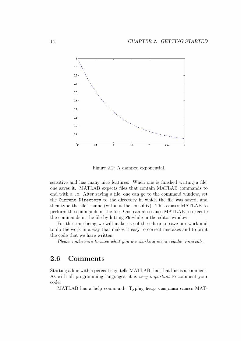
If one gives MATLAB the command plot(t,a), then MATLAB plotsthe vector a against the vector t. Suppose that one gives MATLAB thecommands

2.5. USING THE EDITOR 13
Figure 2.1: A very simple plot
t = 0:0.1:3;
a = exp(-t);
plot(t, a)
Then MATLAB will respond with the graph of Figure 2.2. There are twopoints to note in the code given above. First of all the use of a semi-colonat the end of a line causes MATLAB to suppress the printing of the resultof the assignment. When one is dealing with vectors with tens, hundreds,or thousands of elements this is very helpful. Secondly, the function exp
calculates e to the power given as the argument of the function. As theexample demonstrates, the exp function is vectorized.
2.5 Using the Editor
One can open the MATLAB editor either by typing edit at the MATLABcommand prompt or by clicking on the blank page on the toolbar on theMATLAB window. (If one would like to open a file in the editor, then oneclicks on the folder on the toolbar, selects the relevant file, and then clickson it. MATLAB will open the file in the editor.) The editor is context
14 CHAPTER 2. GETTING STARTED
Figure 2.2: A damped exponential.
sensitive and has many nice features. When one is finished writing a file,one saves it. MATLAB expects files that contain MATLAB commands toend with a .m. After saving a file, one can go to the command window, setthe Current Directory to the directory in which the file was saved, andthen type the file’s name (without the .m suffix). This causes MATLAB toperform the commands in the file. One can also cause MATLAB to executethe commands in the file by hitting F5 while in the editor window.
For the time being we will make use of the editor to save our work andto do the work in a way that makes it easy to correct mistakes and to printthe code that we have written.
Please make sure to save what you are working on at regular intervals.
2.6 Comments
Starting a line with a percent sign tells MATLAB that that line is a comment.As with all programming languages, it is very important to comment yourcode.
MATLAB has a help command. Typing help com_name causes MAT-

2.7. EXERCISES 15
LAB to respond with information about the command. If one writes a file,places comments at the very beginning of the file, and types help filename,MATLAB prints the comments that appear at the beginning of the file. Thisallows the user to “expand” the MATLAB help facility.
2.7 Exercises
1. Recall that the Cauchy-Schwarz inequality states that for any two vec-tors, ~x and ~y, the absolute value of the dot (scalar) product of the twovectors is less than or equal to the product of the norms of the twovectors. Moreover, equality is attained if and only one of the vectors isa multiple of the other vector.
(a) Define the three “vectors”
• ~a = [ 1 2 3 4 5 ]
• ~b = [ 1 3 5 7 9 ]
• ~c = [ 2 4 6 8 10 ]
• Calculate the dot products of ~a with ~b, of ~a with ~c, and of ~bwith ~c.
• Calculate the norms of each of the vectors.
• Verify the Cauchy-Schwarz inequality for the three dot prod-uct calculated above.
2. MATLAB treats the command const ./ vect to mean create a newvectors whose elements are const divided by the elements of vect.Using MATLAB and the commands we have seen, calculate
(a)∑100
k=0 k
(b)∑100
k=0 k2
(c)∑100
k=1 1/k
(d)∑100
k=1 1/k2
(e)∑10000
k=1 1/k2
(f) “Bonus question” To what number are the series of 2d and 2etending?
3. “Bonus question” Derive the formula for
N∑k=0
k2.

16 CHAPTER 2. GETTING STARTED
You may wish to consult [1].
4. Plot five periods of the function cos(2πt). Define a vector t with 100elements the first of which is zero.
5. Write a file that expects the variable N to be defined already. Have thecommands in the file cause MATLAB to calculate the sum
N∑k=1
1
k2.
Add comments to the beginning of the file so that typing help file_name
causes MATLAB to explain what the code does.

Chapter 3
Symbolic Calculations UsingMATLAB
3.1 Overview
Though MATLAB was not really designed to handle symbolic calculations, asthe need for such an ability became clear The MathWorks made an arrange-ment with the designers of Maple—which is a symbolic calculation package.MATLAB’s symbolic math toolbox is a sort of “front end” for Maple. Inthis lab, we learn how to perform symbolic calculations using MATLAB.The book [2] is a good general reference for this subject.
3.2 Getting Started
To define a symbolic variable, x, one can either use the command syms x
or x = sym(’x’). The first command is shorter; the second command issomewhat more versatile. One can define other symbols in terms of symbolsthat have already been defined.
If one gives MATLAB the commands
x = sym(’x’)
y = 1/ (1 + x^2)
MATLAB responds with
y =
1/(1+x^2)
17

18 CHAPTER 3. SYMBOLIC CALCULATIONS USING MATLAB
Figure 3.1: The ezplot command at its simplest
The extremely observant reader will note that when MATLAB printed itsoutput here, it did not indent the answer. The symbolic value 1/(1+x^2}
is printed flush with the margin. In general, MATLAB indents numericalvalues but prints symbolic values flush with the margin.
3.3 Plotting Symbolic Functions
MATLAB has a separate command for plotting symbolic functions: ezplot.The simplest way to use ezplot is to give the command ezplot(y). MAT-LAB then plots the function over a default interval. With y as defined above,giving the command ezplot(y) causes MATLAB to respond with Figure 3.1.If one would like to cause ezplot to plot from xmin to xmax, one can use thecommand ezplot(y, [xmin xmax]).
3.4 Substitutions
MATLAB provides a command that allows us to substitute values, symbolicor otherwise, for symbolic values. The command that performs the substitu-

3.5. EXERCISES 19
tion is called subs. To substitute 2 in the y we defined previously, one givesMATLAB the command subs(y, 2). When given this command, MATLABresponds with
ans =
0.2000
Note that, based on the indentation, we find that MATLAB has given us anumeric value—and not a symbolic one. It is possible to tell MATLAB thatour intention is to substitute the symbol 2—and not some representation of 2.(That is, we tell MATLAB to use an “ideal” 2 and to try to keep everythingas ideal as possible.) To do this one uses sym(’2’) rather than 2. GivingMATLAB the command subs(y, sym(’2’)) causes MATLAB to respondwith
ans =
1/5
Note that the answer here is not indented. MATLAB knows that the symbolit is giving is the correct and precise value it should be returning.
It is also possible to have MATLAB substitute one symbolic value foranother. The command subs(y,x^2), for example, causes MATLAB torespond with
ans =
1/(1+x^4)
3.5 Exercises
1. Define the symbolic variable x. Make use of this variable to definethe symbolic function sin(1/x). Then, plot the function from 0 to 2π.What do you see? Why might the plotting routine be having troubleplotting this function?
2. (Odd and even functions.) To break a function, f(x), into odd andeven parts, one can compute the two functions
fodd(x) =f(x)− f(−x)
2
feven(x) =f(x) + f(−x)
2.

20 CHAPTER 3. SYMBOLIC CALCULATIONS USING MATLAB
You will now perform these operations using MATLAB and examinethe resulting functions.
(a) Define the symbolic variable x.
(b) Define the symbolic function y = ex (using the appropriate MAT-LAB commands).
(c) Define the symbolic function z = e−x by making a substitution inthe symbolic function you found in the previous section.
(d) Using the results of the previous two sections, calculate fodd(x)and feven(x) for the function y = ex.
(e) Use ezplot to plot the functions that you found over the region[−1, 1].
3. Let us evaluate sin(x) at the points π, . . . , 5π again.
(a) Define the symbolic vector a by giving the command
a = sym(’1’):sym(’5’).
This command should give you an array of five “ideal” numbers.
(b) Define the symbol p = sym(’pi’). This command gives you avariable, p, that holds an ideal π.
(c) Now have MATLAB calculate the values of sin(π), . . . , sin(5π) us-ing a single command.
(d) What is the command’s output? Why does it differ from thevalues found in §2.2.
4. (Calculus using the symbolic toolbox) The symbolic toolbox has manycommands that allow one to calculate sums, derivatives and integralsof symbolic quantities. In this exercise we demonstrate a few of thetoolbox’s abilities.
(a) The command symsum causes MATLAB to sum a symbolic expres-sion. Give MATLAB the command symsum(1/sym(’n’)^2,1,inf).That is, have MATLAB calculate
∞∑n=1
1
n2.
Compare this with the values found in exercises 2d and 2e ofChapter 2.

3.5. EXERCISES 21
(b) Calculate the indefinite integral of 1/(1+t2) by using the symbolicintegration command, int.
(c) Calculate the integral ∫ ∞
−∞e−x2/2 dx
by using the command int(funct, low_lim, upper_lim). Pleasenote that inf is the “ideal” infinity and -inf is the ideal negativeinfinity.

22 CHAPTER 3. SYMBOLIC CALCULATIONS USING MATLAB

Chapter 4
Convolution Using theSymbolic Toolbox
4.1 Overview
In this chapter we describe how to use the symbolic toolbox to calculate theconvolution of two functions. As we will see, such calculations seem to be onthe border of what the symbolic toolbox is capable of performing.
4.2 An Easy to Perform Convolution
Let us consider the convolution of 1/(1 + t2) with itself. That is, let uscalculate ∫ ∞
−∞
1
1 + τ 2
1
1 + (t− τ)2dτ.
To do this, we give MATLAB the commands
syms t tau
f = 1/(1 + t^2)
z = int(subs(f,tau)*subs(f,t-tau),tau,-inf,inf)
z = simplify(z)
figure(1)
ezplot(f)
figure(2)
ezplot(z)
MATLAB responds with
f =
23

24 CHAPTER 4. CONVOLUTION USING THE SYMBOLIC TOOLBOX
Figure 4.1: The graph of the function 1/(1 + t2)
1/(1+t^2)
z =
2*pi*t^2/(t^4+4*t^2)
z =
2*pi/(t^2+4)
and Figures 4.1 and 4.2. (The command simplify(z) causes MATLAB tosimplify the symbolic expression given by z, and the command figure(num)
causes MATLAB to open a figure window which it numbers num.)
The calculation of the integral makes use of the int command. Thiscommand performs symbolic integration. As we have used it, the first ar-gument is the function being integrated. The second argument is the vari-

4.2. AN EASY TO PERFORM CONVOLUTION 25
Figure 4.2: The graph of the function 1/(1 + t2) convolved with itself

26 CHAPTER 4. CONVOLUTION USING THE SYMBOLIC TOOLBOX
able over which the integration is to be performed. The third and fourtharguments are the limits of integration. There are many simpler forms ofthe command. Making use of the MATLAB help command, one can findout quite a bit about the command. (The general form of the help com-mand is help command_name. To find out more information about int,type help int.) MATLAB responds to the above commands with all thefunctions—in functional form—and with the graphs of the functions.
4.3 An Exercise
Now we perform a convolution that is more difficult to perform using MAT-LAB. We consider the convolution of the unit step function with itself.
MATLAB does not have a built-in unit step function. Thus, we mustdesign it ourselves. We start by putting together a signum function—a func-tion that returns a one if its input is positive and a minus one if its input isnegative. To do this, we give MATLAB the commands
syms x
sig = x / abs(x)
This looks a bit nasty, but it is pretty clear that for all positive numbers itsoutput is one and for all negative numbers its output is minus one. Try usingezplot to plot the function. If using the simplest form does not work, tryproviding ezplot with the region as well.
Next, we define the step function in terms of the function we have alreadycreated. It is clear that the command
st = (sig + 1)/2
will do the trick. Please plot this function as well.Having defined the step function, we must calculate the convolution. To
do this we give the commands
syms xi
ramp = int(subs(st,xi) * subs(st,x - xi), xi, -inf, inf)
At this point (at least when using MATLAB 6.5), MATLAB flatly refusesto allow ezplot to plot the function. One work-around is to use the subs
command to substitute values into the symbolic function and then to plotthe values. Giving MATLAB the commands
t = [-9.9:0.2:9.9];
a = subs(ramp, t);
plot(t,a)

4.4. EXERCISES 27
Figure 4.3: The result of the convolution in graphical form
causes MATLAB to respond with plot given in Figure 4.3. The functiongiven in the figure, a ramp, is the correct answer.
4.4 Exercises
1. Please calculate the convolution of §4.2 analytically. (You may wantto use residues or Fourier transforms.)
2. Using the symbolic toolbox and the tricks of this chapter, have MAT-LAB calculate and plot the convolution of a unit pulse,
u(t) =
{1, 0 ≤ t < 10, otherwise
,
with itself.

28 CHAPTER 4. CONVOLUTION USING THE SYMBOLIC TOOLBOX
Chapter 5
Solving Differential Equations
5.1 Overview
In this chapter we describe several ways of solving differential equations usingMATLAB. We make use of the symbolic toolbox when possible, and we alsouse numerical methods when desirable. Finally, we show how to use thesetools to evaluate the behavior of a linear time-invariant (LTI) system.
5.2 Solving Ordinary Differential Equations
Symbolically
MATLAB has a command, dsolve, that solves ordinary differential equations(ODEs) symbolically. One form of the dsolve command is
dsolve(’ODE’,’initial conditions’)
In the ODE string, D is used to represent the first derivative and Dn representsthe nth derivative. To solve the differential equation y′(t) = ay(t) subjectto the initial condition y(0) = c and assign the solution to y, one gives thecommands
syms a c
y = dsolve(’Dy = a*y’,’y(0) = c’)
MATLAB replies with
y =
c*exp(a*t)
It is possible to solve much more complicated differential equations this way.
29

30 CHAPTER 5. SOLVING DIFFERENTIAL EQUATIONS
5.3 An Introduction to Matrices
Our next major goal is to solve differential equations numerically. In orderto do this, we will make use of matrices as well as vectors. If one would likeMATLAB to “create” the M ×N dimensional matrix
A =
a11 · · · a1N...
......
aM1 · · · aMN
,
One gives MATLAB the command
A = [a11 ... a1N; ... ; aM1 ... AMN]
That is, one lists the elements of each row separating the elements by spaces(or commas) and separating the rows by semicolons.
If one gives MATLAB the command A = [1 0; 0 1], MATLAB re-sponds with
A =
1 0
0 1
Though many of the commands provided by MATLAB do not care whethera vector is a column vector or a row vector, when using matrices the differenceis critical. If one defines a vector using the command a = [1 2 3], one hasdefined a three-element row vector. To define a column vector, one separateseach element by using a semicolon. If, for example, one gives MATLAB thecommand v = [1; 2; 3], then MATLAB responds with
v =
1
2
3
One can use MATLAB as a simple matrix calculator without defining thematrices and vectors “variables” first. If, for example, one needs to calculate 1 2 3
4 5 67 8 9
1
23
one gives MATLAB the commands

5.4. LOOPING IN MATLAB 31
[1 2 3; 4 5 6; 7 8 9] * [1; 2; 3]
and MATLAB responds with
ans =
14
32
50
(Once again, note that when one would like MATLAB to multiply to objects,one must tell MATLAB to multiply the objects by using an asterisk (*).)
To access the elements of a matrix, one gives the matrix’s name and theposition of the element to be accessed. To access Amn, one types A(m,n).To access the elements of a vector, type the vectors name and the numberof the element. In order to access the second element of the ans vector, forexample, one types ans(2). To this command, MATLAB responds with
ans =
32
(It is worth noting that this new ans variable has overwritten the old ans
vector.)MATLAB has many, many commands for matrix manipulation. To list
just a few:
• inv(A) which inverts the (previously defined) matrix A.
• A^2 which calculates A2.
• More generally, A^N which calculates AN .
• A’ which calculates the conjugate transpose of the matrix A.
For still more matrix operations, give MATLAB the command help elmat
or help matfun.
5.4 Looping in MATLAB
When one is programming, it is often necessary to perform a set of instruc-tions many times. One way to do this is to use some form of loop. MATLABhas a very simple for loop.
The structure of the for loop is

32 CHAPTER 5. SOLVING DIFFERENTIAL EQUATIONS
for var = expression
command1
.
.
.
commandN
end
The expression is a row vector. If one starts a loop with for i = 1:10,then one is “asking” MATLAB to loop through the following commands untilthe matching end is hit. On the first loop, i will be one. On the tenth it willbe 10. Note that indenting the contents of the loop is not necessary, but itmakes the code easier to read. The MATLAB editor generally indents thecontents of a loop.
As a simple example, to have MATLAB calculate ten factorial, one cangive MATLAB the commands
out = 1;
for i = 2:10
out = out * i;
end
out
MATLAB will respond with
out =
3628800
which is indeed 10!.
5.5 Solving Differential Equations Numerically–
A Very Brief Introduction
Consider the equation
d
dty(t) = ay(t) + x(t), y(0) = α.
Let xk = x(kTs), k ≥ 0. Considering the definition of the derivative, it isnot unreasonable to hope that if Ts is sufficiently small, then the sequence

5.6. CONVERTING A HIGH-ORDER ODE INTO A FIRST-ORDER ODE33
{yk} defined by
≈ dydt︷ ︸︸ ︷
yk+1 − yk
Ts
= ayk+1 + xk+1, y0 = α, k ≥ 0
will tend to {y(kTs)}. That is, for small Ts we should find that yk ≈ y(kTs).If Ts is small enough, the sequence should provide a good approximation tothe solution of the differential equation.
Consider, for example, the equation y′ = y, y(0) = 1. Clearly, the exactsolution of this equation is y(t) = et. Rewriting our approximation, we findthat the sequence we are looking for satisfies
yk+1 = yk + Tsyk+1, y0 = 1.
Let us take Ts = 0.1.The following code calculates the approximation. In this code yk is the
k + 1th element of the vector y. This is done because MATLAB does notallow a vector to start from element zero; all vectors start from element 1.
y(1) = 1;
for i = 2:11
y(i) = y(i-1)/(1 - 0.1);
end
plot(0:0.1:1, y, 0:0.1:1, exp(0:0.1:1))
legend(’The Approximation’,’The Exact Solution’)
MATLAB responds to the commands with the plot of Figure 5.1. (Thelegend command causes MATLAB to add a legend to the plot. Use theMATLAB help command to find out more about the legend command.)
5.6 Converting a High-order ODE into a First-
order ODE
Suppose that one would like to write the second order ODE
y′′ + y′ + y = 0, y(0) = 1, y′(0) = 0
as a set of first order ODEs. One can proceed as follows. Define:
~x(t) =
[y(t)y′(t)
].

34 CHAPTER 5. SOLVING DIFFERENTIAL EQUATIONS
Figure 5.1: A comparison of the exact and the approximate solutions of thedifferential equation.
5.6. CONVERTING A HIGH-ORDER ODE INTO A FIRST-ORDER ODE35
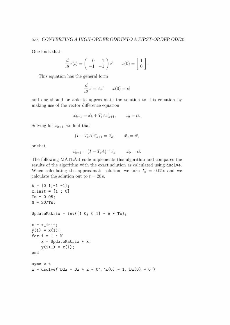
One finds that:
d
dt~x(t) =
(0 1
−1 −1
)~x ~x(0) =
[10
].
This equation has the general form
d
dt~x = A~x ~x(0) = ~α
and one should be able to approximate the solution to this equation bymaking use of the vector difference equation
~xk+1 = ~xk + TsA~xk+1, ~x0 = ~α.
Solving for ~xk+1, we find that
(I − TsA)~xk+1 = ~xk, ~x0 = ~α,
or that~xk+1 = (I − TsA)−1~xk, ~x0 = ~α.
The following MATLAB code implements this algorithm and compares theresults of the algorithm with the exact solution as calculated using dsolve.When calculating the approximate solution, we take Ts = 0.05 s and wecalculate the solution out to t = 20 s.
A = [0 1;-1 -1];
x_init = [1 ; 0]
Ts = 0.05;
N = 20/Ts;
UpdateMatrix = inv([1 0; 0 1] - A * Ts);
x = x_init;
y(1) = x(1);
for i = 1 : N
x = UpdateMatrix * x;
y(i+1) = x(1);
end
syms z t
z = dsolve(’D2z + Dz + z = 0’,’z(0) = 1, Dz(0) = 0’)

36 CHAPTER 5. SOLVING DIFFERENTIAL EQUATIONS
Figure 5.2: A comparison of the exact and the approximate solutions of thedifferential equation.
time = [0 : N] * Ts;
z_eval = subs(z,t,time);
plot(time, y, ’-’, time, z_eval, ’--’)
legend(’The numerical solution’,’The solution as provided by dsolve’)
The code’s output is given in Figure 5.2
5.7 ODEs, Transfer Functions, and the Step
Response
Let us use the knowledge we now have to calculate the step response of theblock whose transfer function is
G(s) =1
τs + 1
in two different ways. First, we solve the relevant equations analytically usingthe dsolve command. Then, we solve the equations numerically.

5.8. THE NUMERICAL SOLUTION 37
5.7.1 The Analytical Solution
Let Y (s) be the Laplace transform of the output of the system, and let X(s)be the Laplace transform of the input of the system. Then, we know that
Y (s)
X(s)=
1
τs + 1.
Cross-multiplying, we find that
τsY (s) + Y (s) = X(s).
Converting back to a differential equation, we find that
τy′(t) + y(t) = x(t).
Recall that when calculating the step response of a system we assume thatall relevant initial conditions are zero and the input, x(t), is 1 for t ≥ 0.
We find that in order to calculate the step response, we must solve theODE
τy′(t) + y(t) = 1
subject to the initial condition y(0) = 0. Making use of the symbolic toolboxby giving MATLAB the commands
syms tau y t
step = dsolve(’tau * Dy + y = 1’, ’y(0) = 0’)
causes MATLAB to respond with
step =
1-exp(-1/tau*t)
5.8 The Numerical Solution
To solve this equation numerically, we make use of the approximation
yk+1 − yk
Ts
≈ y′((k + 1)Ts).
Making use of this approximation, we find that the ODE can be approximatedby the difference equation
τ
Ts
(yk+1 − yk) + yk+1 = 1, y0 = 0.
Translating this equation into MATLAB code and choosing Ts = 0.01 andτ = 0.5, we find that giving MATLAB the commands
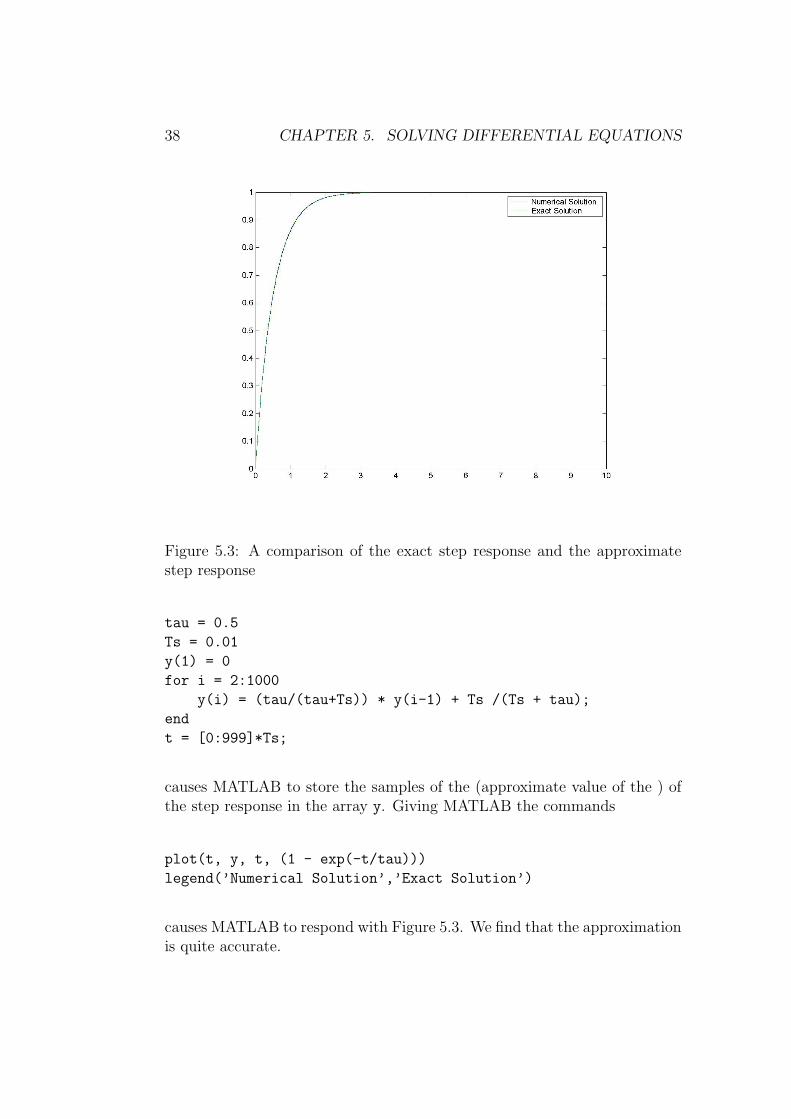
38 CHAPTER 5. SOLVING DIFFERENTIAL EQUATIONS
Figure 5.3: A comparison of the exact step response and the approximatestep response
tau = 0.5
Ts = 0.01
y(1) = 0
for i = 2:1000
y(i) = (tau/(tau+Ts)) * y(i-1) + Ts /(Ts + tau);
end
t = [0:999]*Ts;
causes MATLAB to store the samples of the (approximate value of the ) ofthe step response in the array y. Giving MATLAB the commands
plot(t, y, t, (1 - exp(-t/tau)))
legend(’Numerical Solution’,’Exact Solution’)
causes MATLAB to respond with Figure 5.3. We find that the approximationis quite accurate.

5.9. EXERCISES 39
5.9 Exercises
1. Use the dsolve command to solve the differential equation y′′(t) =−y(t) subject to the initial conditions y(0) = 1, y′(0) = 0. Use theMATLAB help command (type help dsolve) if you need help withthe commands syntax. Plot the solution using the ezplot command.
2. Use the dsolve command to solve the differential equation y′′(t) =−2y′(t)− y(t) subject to the initial conditions y(0) = 1, y′(0) = 0. Plotthe solution using the ezplot command.
3. Define the matrix
A =
1 2 53 7 91 5 9
and the vector ~v,
~v =
159
Calculate A~v, A2~v, and A−1~v.
4. Use MATLAB to approximate the solution of the equation y′′(t) =−y(t) subject to the initial conditions y(0) = 1, y′(0) = 0. Comparethe approximate solution to the exact one found in exercise 1.
5. Use MATLAB to calculate the step response of the system whose trans-fer function is
G(s) =1
s2 + s + 1
(a) Derive the differential equation satisfied by the step response.
(b) Use the dsolve command to solve the ODE.
(c) Next, approximate the solution of the ODE using the techniqueswe have studied.
(d) Compare the solutions of parts 5b and 5c.

40 CHAPTER 5. SOLVING DIFFERENTIAL EQUATIONS
Chapter 6
Fourier Series and the GibbsPhenomenon
6.1 The Fourier Series of the Square Wave
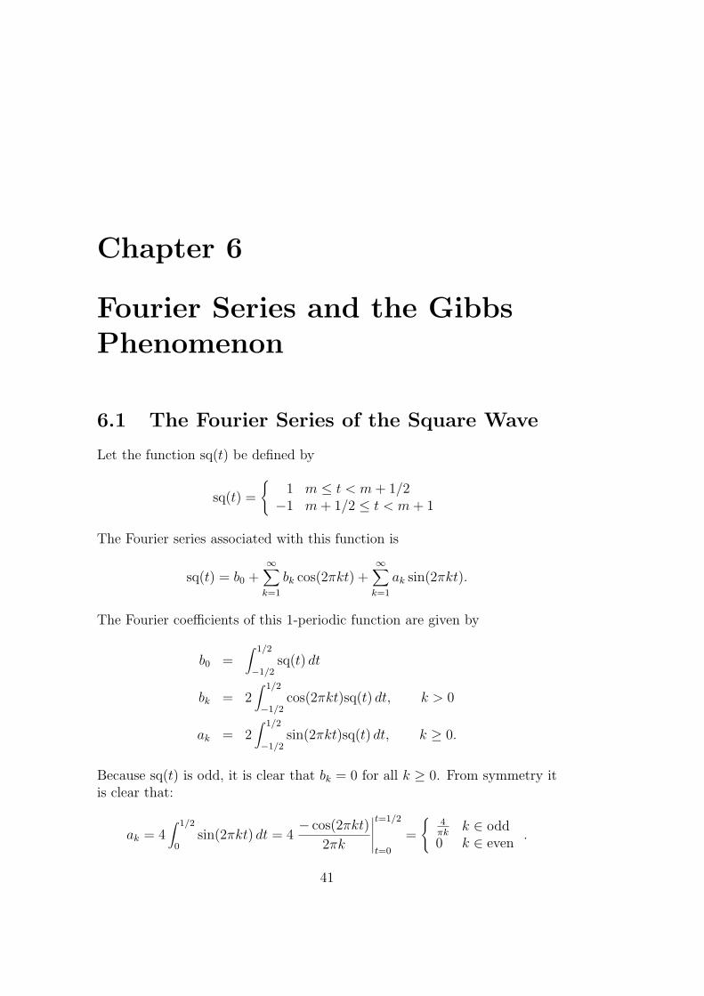
Let the function sq(t) be defined by
sq(t) =
{1 m ≤ t < m + 1/2
−1 m + 1/2 ≤ t < m + 1
The Fourier series associated with this function is
sq(t) = b0 +∞∑
k=1
bk cos(2πkt) +∞∑
k=1
ak sin(2πkt).
The Fourier coefficients of this 1-periodic function are given by
b0 =∫ 1/2
−1/2sq(t) dt
bk = 2∫ 1/2
−1/2cos(2πkt)sq(t) dt, k > 0
ak = 2∫ 1/2
−1/2sin(2πkt)sq(t) dt, k ≥ 0.
Because sq(t) is odd, it is clear that bk = 0 for all k ≥ 0. From symmetry itis clear that:
ak = 4∫ 1/2
0sin(2πkt) dt = 4
− cos(2πkt)
2πk
∣∣∣∣∣t=1/2
t=0
=
{4
πkk ∈ odd
0 k ∈ even.
41

42 CHAPTER 6. FOURIER SERIES AND THE GIBBS PHENOMENON
Thus, we find that the Fourier series associated with sq(t) is∞∑
k=0
4 sin(2π(2k + 1)t)
π(2k + 1).
We would now like to examine the extent to which this series truly representsthe square wave.
6.2 A Quick Check
Before proceeding to analyze the series we have found, it behooves us to checkthat the calculations were performed correctly. For a 1-periodic function likesq(t), Parseval’s equation states that∫ 1/2
−1/2sq2(t) dt = b2
0 +1
2
∞∑k=1
(a2k + b2
k).
In our case this means that
1 =1
2
∞∑k=0
(4
π(2k + 1)
)2
=8
π2
∞∑k=0
1
(2k + 1)2.
We can check that this sum is correct using MATLAB. One way to per-form a quick check is to give MATLAB the commands
L = [1:2:10001];
(8/pi^2) * sum(1./L.^2)
MATLAB responds with
ans =
1.0000
which is an indication that we may have performed all of the calculationscorrectly.
A second way to have MATLAB check this computation is to give MAT-LAB the commands
syms k
(sym(’8’)/sym(’pi’)^2) * symsum(1/(2*k+1)^2,k,0,Inf)
MATLAB responds to these commands with
ans =
1
indicating that the series does, indeed, sum to 1.

6.3. “SEEING” THE SUM 43
Figure 6.1: Summing the Fourier series. The “ringing” associated with Gibb’sphenomenon is clearly visible.
6.3 “Seeing” the Sum
It is not difficult to have MATLAB calculate the Fourier series and displayits values. Conisder the following code:
t = [-500:500] * 0.001;
total = zeros(size(t));
for k = 1 : 2 : 101
total = total + (4/pi) * sin(2*pi*k*t) / k;
end
plot(t,total)
This code defines a “time” vector, t, with 1001 elements. It then defines avector to hold the sum, total, and proceeds to sum the first 51 terms inthe Fourier series. The code causes MATLAB to produce the plot shown inFigure 6.1. The “ringing” produced by Gibb’s phenomenon is clearly visible.
44 CHAPTER 6. FOURIER SERIES AND THE GIBBS PHENOMENON
6.4 The Experiment
Letsaw(t) = t
for −1/2 < t ≤ 1/2 and continue saw(t) periodically outside of this region.
1. Calculate the Fourier coefficients associated with saw(t).
2. Check Parseval’s equation for saw(t) both numerically and symboli-cally.
3. Sum the first 3 terms in the Fourier series and plot the Fourier seriesas a function of time.
4. Sum the first 10 terms in the Fourier series and plot the Fourier seriesas a function of time.
5. Sum the first 50 terms in the Fourier series and plot the Fourier seriesas a function of time.
When summing the Fourier series, make sure that the time samples you takeare sufficiently closely spaced that you clearly see Gibb’s phenomenon.

Chapter 7
Linearity and Nonlinearity
7.1 Linearity
Suppose that when one inputs x1 to a system, the output of the system isy1, and when one inputs x2 to a system, the output of the system is y2. Asystem is said to be linear if from these two facts one can conclude that ifthe input to the system is α1x1 +α2x2, then the output of the system will beα1y1 +α2y2. Linear systems are said to satisfy the principle of superposition.
7.2 Simulink
To “see” when a system is linear and when it is not, we make use of Simulink—a MATLAB “add-on.” Simulink is, essentially, a graphical user interface(GUI) to MATLAB. It allows one to drag-and-drop blocks to build up asystem.
To open Simulink, one can type “simulink” at the MATLAB commandprompt. Alternatively one can click on the Simulink icon on the toolbar inthe main MATLAB window.
After performing either of these actions, the Simulink Library Browserwill open. After it has opened, click on the blank page in this window’stoolbar to open a new Simulink “page.” To start working, one drags anddrops items from the library browser into the worksheet, one connects theitems, and then one runs the simulation.
45

46 CHAPTER 7. LINEARITY AND NONLINEARITY
7.3 A Simple Example
We start by building a system that amplifies a sine wave by a factor of two.To do this, go to the browser, click on the “sources” tab (in the Simulink“blockset”), and then drag a “sine wave” over to the untitled worksheet.
Having actually put something in the worksheet, it is probably best tosave the worksheet; do so. Note that Simulink saves its worksheets with a.mdl extension. (Make sure to save worksheets regularly while working onthem.)
Next, go to the “Math Operations” tab, click on it and drag a gain blockto the worksheet. To connect the sine wave to the gain block select the sinewave block, hold down the control key and left-click on the gain block. (Thisis the general procedure for connecting blocks.)
Go to the “Sinks” tab, click on it, and drag a Scope block from the right-hand panel to the worksheet. Then connect the gain block to the scope.Double click on the gain block, and use the dialog box that opens to changethe gain of the gain block from 1 to 2. Double click on the sine wave block,and change its frequency from 1 radian per second to 2π radians per second.(Enter 2 * pi as the frequency.) Double click on the scope to actually open ascope window. Finally hit the “play” button on top of the worksheet window,and a sine wave should appear in the scope window.
The sine wave may not be very pretty. Simulink is numerical software,and it is not always good at “guessing” how many samples of a function theuser needs. In our case, in order to improve the quality of the sine wave,one can click on the sine wave block again and change the sample time fromzero—which is “continuous-time”—to 0.001 s—which gives lots of samples ineach period of the sine wave. Make the change and hit play again. How doesthe sine wave look now?
7.4 Testing Linearity
We now test the linearity of the gain block. To do this, build the system ofFigure 7.1. The following tips should prove helpful.
• To copy a block, hold down the control key, left-click on the block anddrag the copy to wherever it is needed.
• The summing block (the circle with the pluses inside) is located in the“Math Operations” library.
• Double clicking on the summing block opens up a dialog box that allows

7.4. TESTING LINEARITY 47
Figure 7.1: A system to test the linearity of the gain block

48 CHAPTER 7. LINEARITY AND NONLINEARITY
one to change the sums to differences. That is how one produces adifferencing block.
• To add a connection to a “wire,” hold down the control key, click onthe spot on the wire to which you would like to add a connection, anddrag the cursor to the input of the item to which you would like toconnect. Release the cursor when a double cross-hair is shown over theblock’s input.
• In order to open a scope window, double click on the scope of interest.
• If one does not see the whole signal on a scope, the problem is probablythat the window is limiting the number of samples that it saves. Toremove this restriction, go to the scope window. Go to the “parame-ters” tab (the second tab from the left) and click on it. A dialog boxwill open. Click on the “data history” tab, and unclick the “limit datapoints to last” box.
• Make the frequencies of the two sine waves different.
7.5 A Nonlinear System
Save the model that you have build for the linear system. Pick another blockthat should be nonlinear—perhaps the “sign” block in the “Math Operations”sub-library—and replace all the gains with this block. Run the simulationagain. What is the output of the differencing block? How do your resultsshow that the new block is not linear—that it is non-linear?
7.6 Exercise
1. Use the symbolic toolbox to show that the squaring operation is notlinear. That is, use the symbolic toolbox to show that
(αx + βy)2 6= αx2 + βy2.
You may wish to use the commands pretty and collect to make theresults of the symbolic calculations easier to read and understand. (Usethe help command to find out how to use these new commands.)

Chapter 8
Continuous-time LinearSystems
8.1 Overview
One of the first, if not the first, MATLAB toolboxes was the control theorytoolbox. By using the commands in this toolbox it is possible to define trans-fer function objects and to examine the properties of the systems describedby the transfer functions.
8.2 Defining a Transfer Function Object
To define a transfer function object that corresponds to a transfer functionthat is rational function—a function that is the quotient of polynomials—one gives MATLAB the command tf(num,den). The vector num containsthe coefficients of the numerator polynomial and the vector den contains thecoefficient of the denominator polynomial. The first element of each vectoris the coefficient of the highest power in the polynomial, and each elementafterwards corresponds to the next lower power of s. Suppose that one hasa system for which
G(s) =1
0.1s + 1.
Giving MATLAB the command
G = tf([1],[0.1 1])
cause MATLAB to respond with
Transfer function:
49
50 CHAPTER 8. CONTINUOUS-TIME LINEAR SYSTEMS
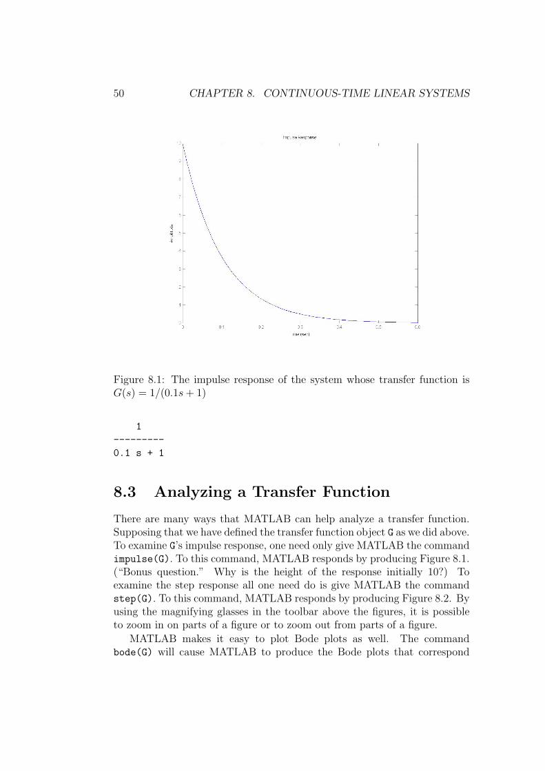
Figure 8.1: The impulse response of the system whose transfer function isG(s) = 1/(0.1s + 1)
1
---------
0.1 s + 1
8.3 Analyzing a Transfer Function
There are many ways that MATLAB can help analyze a transfer function.Supposing that we have defined the transfer function object G as we did above.To examine G’s impulse response, one need only give MATLAB the commandimpulse(G). To this command, MATLAB responds by producing Figure 8.1.(“Bonus question.” Why is the height of the response initially 10?) Toexamine the step response all one need do is give MATLAB the commandstep(G). To this command, MATLAB responds by producing Figure 8.2. Byusing the magnifying glasses in the toolbar above the figures, it is possibleto zoom in on parts of a figure or to zoom out from parts of a figure.
MATLAB makes it easy to plot Bode plots as well. The commandbode(G) will cause MATLAB to produce the Bode plots that correspond

8.3. ANALYZING A TRANSFER FUNCTION 51
Figure 8.2: The step response of the system whose transfer function is G(s) =1/(0.1s + 1)

52 CHAPTER 8. CONTINUOUS-TIME LINEAR SYSTEMS
Figure 8.3: The block diagram of the system in which G(s) and H(s) arecascaded
to the system. If all that one is interested in is the magnitude plot, MAT-LAB provides one with the command bodemag.
For more information about any given command, use the MATLAB help
command.
8.4 Transfer Function Manipulations
Suppose that one is working with the system of Figure 8.3 where
G(s) =1
0.1s + 1and H(s) =
s
0.1s + 1.
As we have already seen, G(s) is the transfer function of a low-pass filter. Itis easy to see that H(s) is the transfer function of a high-pass filter. GivingMATLAB the command
H = tf([1 0],[0.1 1])
causes MATLAB to define the transfer function of the second block.
How will the system behave? If one cascades two blocks, then the transferfunction of the cascaded blocks is the product of the transfer functions ofthe blocks. MATLAB knows how to multiply transfer functions, and givingMATLAB the command T = G*H, causes MATLAB to respond with
Transfer function:
s
--------------------
0.01 s^2 + 0.2 s + 1
Giving MATLAB the command bodemag(T), cause MATLAB to produceFigure 8.4. We find that the cascaded blocks lead to a bandpass filter.

8.4. TRANSFER FUNCTION MANIPULATIONS 53
Figure 8.4: The magnitude plot of the system in which G(s) and H(s) arecascaded

54 CHAPTER 8. CONTINUOUS-TIME LINEAR SYSTEMS
Figure 8.5: A system with feedback
8.5 Systems with Feedback
Considering the system of Figure 8.5 and starting from Vout(s), it is easy tosee that:
Vout(s) = G(s)(Vin(s)−H(s)Vout(s)).
Rearranging terms, we find that
(1 + G(s)H(s))Vout(s) = G(s)Vin(s).
We find thatVout(s)
Vin(s)=
G(s)
1 + G(s)H(s).
This is the transfer function of the system of Figure 8.5.MATLAB is capable of computing the transfer function of the system with
feedback from the trasnfer functions of its constituent parts. For example, ifG(s)1/(s + 1) and H(s) = 2, then giving MATLAB the commands
G = tf([1],[1 1]);
H = tf([2],[1]);
T = G / (1 + G*H)
causes MATLAB to respond with
Transfer function:
s + 1
-------------
s^2 + 4 s + 3
8.6. EXERCISES 55
This is somewhat odd, as a simple calculation shows that the transferfunction of the system with feedback is
T (s) =G(s)
1 + G(s)H(s)=
1
s + 3.
If one considers the answer provided by MATLAB somewhat more carefully,one finds that
s + 1
s2 + 4s + 3=
s + 1
(s + 1)(s + 3)=
1
s + 3.
That is, MATLAB found the correct answer but expressed it in an oddfashion. MATLAB took a first order transfer function and made it look likea second order transfer function.
8.6 Exercises
1. What kind of system is described by the transfer function
G(s) =1
τs + 1?
2. Analyze the system whose transfer function is
G(s) =s
s2 + s + (2π100)2.
(a) Define the transfer function object, G.
(b) Find the impulse response of the system.
(c) Explain the frequency of the oscillations that you see.
(d) Find the step response of the system.
(e) Explain why the step response of the system starts from zero andends at zero.
3. Analyze the system whose transfer function is
G(s) =−s + 1
2s2 + s + 3.
(a) Use the ltiview command to open the ltiviewer—the linear time-invariant system viewer. Use the help command to discover howthis command is used.

56 CHAPTER 8. CONTINUOUS-TIME LINEAR SYSTEMS
(b) Have the ltiviewer display the step and impulse responses of thesystem.
(c) Explain why the step response of the system is initially negative.
4. Consider the system of Figure 8.5. Let H(s) = 1. Have MATLABcalculate the step response of the system described by the figure when:
(a) G(s) = 0.125/(s2 + s)
(b) G(s) = 0.25/(s2 + s)
(c) G(s) = 0.5/(s2 + s)
(d) G(s) = 1/(s2 + s)
What effect does the increased gain have on the system’s performance?(Please address both the system’s rise time and the amount of overshootin the system’s output.)

Chapter 9
Non-minimum-phase Systems
9.1 Overview
Generally speaking, the transfer functions we see have both their poles andtheir zeros in the left half-plane. For causal systems, having a pole in theright half-plane is a big problem. Such a pole indicates that the system isnot stable.
Systems with zeros in the right half-plane are said to be non-minimum-phase systems. What can one say about such systems?
One point that should be immediately obvious is that if G(s) has a zeroin the right half-plane, then 1/G(s) has a pole in the right half-plane andis not the transfer function of a stable system. This means that one cannotbuild a perfect open-loop compensator for G(s). What else can one say aboutnon-minimum-phase systems?
9.2 The Step Response of a Non-minimum-
phase System
Suppose that one has a stable system whose transfer function is G(s) andwhose DC gain, G(0), is positive. Suppose that in addition, G(a) = 0 forsome a > 0; suppose that G(s) has a zero in the right half-plane. Thenwe can show that at some point the step response of the system must gonegative.
On an intuitive level, inputting a value of 1 to a system should causethe system to head towards the positive numbers. Assuming that a system’sinitial conditions are zero, inputting a value of 1 should cause the systemto head in the positive “direction.” We now show that this is not neces-
57

58 CHAPTER 9. NON-MINIMUM-PHASE SYSTEMS
sarily what happens. Non-minimum-phase systems behave in an anomalousfashion.
The output of the system whose transfer function is G(s) to a unit step,vstep(t), satisfies
Vstep(s) =1
sG(s).
From the final value theorem, we know that
limt→∞
vstep(t) = lims→0+
s(
1
sG(s)
)= lim
s→0+G(s) = G(0) > 0.
Thus, we know that the step response converges to a positive value.
We also know that
0 =1
sG(s)
∣∣∣∣s=a
= G(a)/a
=∫ ∞
0e−atvstep(t) dt.
We know that for large enough t the step response is greater than zero, andthe exponential is always greater than zero. In order for the integral to equalzero, the step response must be negative at some point.
9.3 The Experiment: Part I
Define a transfer function object whose transfer function is given by
G(s) =−s/2 + 1
s2 + s/2 + 1
Use the step command to plot the step response of the system. Does thestep response agree with the predictions made by our theory?
9.4 Short-term Vs. Long-term Behavior
In §9.2, we found that if a stable system has a zero or zeros in the right half-plane, then the system’s step response must be negative for some positivevalue of t. In the example of §9.3, we found that the step response startedoff negative and then turned positive. Must this always be the case?

9.5. THE EXPERIMENT: PART II 59
Let us consider transfer functions with a zero or zeros at a > 0, with allother zeros and poles in the left half-plane, and with positive DC gain. Suchtransfer functions must be of the form
G(s) = (a− s)mF (s)
where F (s) has all of its poles and zeros in the left-half plane and F (0) > 0.The initial value theorem states that if H(s) is the Laplace transform of
h(t), thenh(0+) = lim
s→∞sH(s).
In particular, if the degree of the denominator of G(s) is greater than thatof the numerator of G(s), then the initial value of the step response of thesystem described by G(s) will be
initial value = lims→∞
s1
sG(s) = 0.
The Laplace transform of f ′(t) is sF (s)−f(0+). If f(0+) is zero, then theLaplace transform of f ′(t) is sF (s). Considering the step response again, wefind that the Laplace transform of the derivative of the step response is G(s).Assuming that the difference in the degrees of the numerator is exactly one,we find that the initial value of the derivative is
v′step(0) = lims→∞
sG(s) = lims→∞
s(a− s)mF (s).
As the degrees of the numerator and the denominator of sG(s) are the same,the limit will be a non-zero number. As the sign of F (s) is positive for largevalue of s, the sign of the number will be the same as that of (a−s)m. If m iseven, the sign will be positive, and if m is odd, the sign will be negative. Thatis, if m is even, the derivative of the step response is initially positive, andstep response initially increases from 0, then turns negative, and eventuallytends to G(0). If m is odd, then the step response decreases initially.
9.5 The Experiment: Part II
9.5.1 The Step Response
Define a transfer function object that corresponds to a system whose transferfunction is
G(s) =(1− s/2)2
s3 + 6.25s2 + 7s + 1
Have MATLAB plot the step response of the system. Does the plot agreewith theory developed? Explain.

60 CHAPTER 9. NON-MINIMUM-PHASE SYSTEMS
9.5.2 The Derivative of the Step Response
For the G(s) given above, we find that the degree of the denominator is onegreater than the degree of the numerator. As we have already seen, thisimplies that the step response of the system is zero when t = 0 and that thederivative of the step response is G(s).
In order to understand the step response somewhat better, we would liketo cause MATLAB to plot the derivative of the step response. To do this,we need to cause MATLAB to plot the inverse Laplace transform of G(s).This, however, is precisely the impulse response of the system. As we saw in§8.3, MATLAB has a command, impulse, that plots the impulse response.Have MATLAB plot the derivative of the step response.
Now, explain the connection between the plot of the derivative of the stepresponse and the plot of the step response. How does the first plot explainwhat we see in the second plot?
9.6 The Experiment: Part III
It is possible to arrive at the transfer function
G(s) =(1− s/2)2
s3 + 6.25s2 + 7s + 1(9.1)
by considering a system like that of Figure 8.5 and taking
G(s) =(1− s/2)2
s3 + 6s2 + 8s(9.2)
and H(s) = 1.
Define the trasnfer function object G to have the transfer function givenby (9.2). Let T be defined by T = G/(1+G). Note that the resulting transferfunction does not seem to match that of (9.1). Actually, MATLAB hassimply “inflated” the transfer function (as it did in §8.5).
Give MATLAB the command step(T). Examine the region near t = 0carefully. Does the step response of the system rise above zero before dippingbellow zero? Try to explain why the step response as given by MATLABdoes not quite match the step response it gave in the previous section. Thisexample shows that sometimes using the correct form for a function can beimportant to numerical methods used to evaluate the function.

9.7. EXERCISES 61
9.7 Exercises
1. Explain why if the denominator of a function, G(s), is of higher degreethan the numerator of G(s), then
lims→∞
G(s) = 0.
2. Let u(t) be the unit step function. Let g(t) be a system’s impulseresponse, and let G(s), the Laplace transform of g(t), be the system’stransfer function. By definition, the step response of a system is theoutput of the system when the input is u(t). For our system,
vstep(t) =∫ ∞
−∞u(t− τ)g(τ) dτ.
Differentiate this function, and show that v′step(t) = g(t). (You mayassume that any calculation that looks “legal” is.)

62 CHAPTER 9. NON-MINIMUM-PHASE SYSTEMS

Chapter 10
Analog Filter Design UsingMATLAB
10.1 Overview
MATLAB provides many filter design tools. Most of the tools are aimed atdigital filter design, but some of the tools also support analog filter design.We briefly consider some analog filter design tools.
10.2 Designing a Butterworth Filter
To design an analog low-pass Butterworth filter using MATLAB, one usesthe command
[b a] = butter(order, cutoff_freq, ’s’)
This command tells MATLAB to design a low-pass Butterworth filter oforder order and cutoff frequency cutoff_freq. The ’s’ tells MATLAB todesign an analog filter. (Without this command, MATLAB designs a digitalfilter.) The vectors a and b hold the coefficients of the denominator and thenumerator (respectively) of the filter’s transfer function. Giving MATLABthe commands
[b a] = butter(4, 100, ’s’);
G = tf(b,a)
causes MATLAB to respond with
63

64 CHAPTER 10. ANALOG FILTER DESIGN USING MATLAB
Figure 10.1: The magnitude plot of the fourth-order low-pass Butterworthfilter with a cutoff frequency of 100 rad/s.
Transfer function:
1e008
-----------------------------------------------------
s^4 + 261.3 s^3 + 3.414e004 s^2 + 2.613e006 s + 1e008
Giving MATLAB the command bodemag(G,{30,3000}) causes MATLAB torespond with Figure 10.1. (The term {30,3000} in the bodemag commandcauses the command to plot the magnitude response from 30 rad/s out to3,000 rad/s.)
Two points are worth noting. Looking at the magnitude plot, one seesthat at 100 rad/s the response seems to have decreased by about 3 dB—asit should. Also, one notes that from 100 rad/s to 1,000 rad/s the responseseems to drop by about 80 dB. As this is a fourth order filter its rolloff shouldbe 4× 20 dB/dec.

10.3. EXERCISES 65
10.3 Exercises
1. Design a fourth order high-pass Butterworth filter whose cutoff fre-quency is 1,000 rad/s.
(a) What is the transfer function of the filter?
(b) Plot the magnitude response of the filter.
(c) What is the high-frequency rolloff?
2. Compare the performance of a fourth-order low-pass Chebyshev filterwith a cutoff frequency of 1 kHz with the performance of Butterworthfilter of the same order.
(a) Use the MATLAB help command to learn how to use the cheby2command.
(b) Use the commands butter and cheby2 to design the two filters.
(c) Plot the magnitude plots of the two filters.
(d) Which of the filters has a narrower transition region?
(e) Which of the filters has a “prettier” magnitude response?

66 CHAPTER 10. ANALOG FILTER DESIGN USING MATLAB

Chapter 11
Using MATLAB to CalculateTransforms
11.1 The Fourier Transform
In principle, calculating Fourier transforms using the symbolic toolbox shouldnot be too hard. In practice it seems to require a fair amount of thought andeffort.
Consider the Fourier transform of a pulse—of a function of the form:
Πa(t) =
{1 |t| ≤ a/20 otherwise
.
In principle, calculating the transform should be simple. All that one needsto do is to calculate the integral of e−2πjftΠa(t) with respect to t. In practice,one must first define the pulse function.
One way to define the function is to give MATLAB the commands
syms t a
sgn = t/abs(t)
stp = (sym(’1’) + sgn)/sym(’2’)
pulse = subs(stp,t+a/sym(’2’)) - subs(stp,t-a/sym(’2’))
MATLAB responds with
pulse =
1/2*(t+1/2*a)/abs(t+1/2*a)-1/2*(t-1/2*a)/abs(-t+1/2*a)
If one would like to see this in a more human-readable form, one can giveMATLAB the command pretty(pulse). MATLAB responds with
67

68 CHAPTER 11. USING MATLAB TO CALCULATE TRANSFORMS
t + 1/2 a t - 1/2 a
1/2 ------------- - 1/2 --------------
| t + 1/2 a | | -t + 1/2 a |
The symbol pulse is just what we need. To calculate the Fourier trans-form of Π1(t), we give MATLAB the commands
j = sqrt(sym(’-1’))
pulse_trans = int(exp(-2*pi*j*f*t) * subs(pulse,a,1), t, -inf, inf)
MATLAB responds with
-1/2*i*(-exp(-i*pi*f)+exp(i*pi*f))/pi/f
To simplify this expression and present it in a more human-readable form,one can use the command pretty(simple(pulse_trans)). The simple
command looks for a simple form of pulse_trans, and, as we have seen, thepretty command presents the results in a more human-readable form. Theresults MATLAB gives are
sin(pi f)
---------
pi f
This is both a pretty and a simple form of the transform.To plot this function one could use the ezplot command. For some
reason, this does not seem to give optimal results. It is also possible to givethe commands
t = -20.005:0.01:20.005;
out = subs(pulse_trans,t);
plot(t,out,t,zeros(size(t)))
axis tight
These commands cause MATLAB to respond by producing Figure 11.1. (Thereason for the somewhat odd-looking definition of t—the set of points atwhich the Fourier transform is to be evaluated—is to avoid having any ele-ment of t equal to zero. Evaluating
sin(πf)
πf
at f = 0 causes MATLAB to generate a divide-by-zero error.)The command axis tight causes MATLAB to make the border of the
figure fit the plotted values “tightly.” The command zeros(size(obj))

11.2. Z-TRANSFORMS 69
Figure 11.1: The Fourier transform of Π1(t)
causes MATLAB to generate a new object all of whose elements are zero andthat has the same dimensions as obj. The plot command used here causesMATLAB to plot the values of out against those of t and then to plot thevalues of zeros(size(t)) against those of t. This is what produced the liney = 0.
11.2 Z-transforms
Calculating the Z-transform can be done by using the symsum command.This command calculates sums of symbolic random variables and is verysimilar to the int command.
Let us calculate the Z-transform of the sequence
ak =
{kTs k ≥ 00 otherwise
To do this and cause MATLAB to output the results in an eye-pleasingfashion, we give MATLAB the commands
syms k Ts z

70 CHAPTER 11. USING MATLAB TO CALCULATE TRANSFORMS
trans = symsum(Ts * k * z^(-k),k,0,inf);
pretty(trans)
MATLAB responds with
Ts z
---------
2
(-1 + z)
11.3 Exercises
1. Show that the expression
t + 1/2 a t - 1/2 a
1/2 ------------- - 1/2 --------------
| t + 1/2 a | | -t + 1/2 a |
is, in fact, equal to Πa(t). You may want to examine the value of theexpression when t < −a/2, when −a/2 ≤ t < a/2, and when t ≥ a/2.
2. Make use of the symbolic toolbox to calculate the Fourier transform of
g(t) =
{e−t t ≥ 00 otherwise
3. Make use of the symbolic toolbox to calculate the Fourier transform of
g(t) = e−|t|.
It may be necessary to calculate the Fourier transform of g(t) by cal-culating the integral from −∞ to 0 and from 0 to ∞ separately. Then,of course, one must add the two results to get the final result.
4. Make use of the techniques of §11.1 to calculate and plot the Fouriertransform of Π1(t) cos(2π100t).
5. Make use of the symbolic toolbox to calculate the Z-transform of thesequences:
(a)
ak =
{k2 k ≥ 00 otherwise
(b) ak = b−|k|

Bibliography
[1] Courant, R. and Robbins, H., What is Mathematics?, Oxford UniversityPress, 1996.
[2] The MathWorks, Inc., Symbolic Math Toolbox, Version 3.1.
[3] Moler, C., “The Origins of MATLAB,” video clip,http://www.mathworks.com/company/aboutus/founders/clevemoler.html
71