a maximum entropy approach to adaptive statistical language
TRANSCRIPT

Computer Speech and Language (1996) 10, 187–228
A maximum entropy approach to adaptivestatistical language modelling
Ronald RosenfeldComputer Science Department, Carnegie Mellon University, Pittsburgh,
PA 15213, U.S.A., e-mail: [email protected]
Abstract
An adaptive statistical language model is described, which successfullyintegrates long distance linguistic information with other knowledgesources. Most existing statistical language models exploit only theimmediate history of a text. To extract information from further backin the document’s history, we propose and use trigger pairs as thebasic information bearing elements. This allows the model to adapt itsexpectations to the topic of discourse. Next, statistical evidence frommultiple sources must be combined. Traditionally, linear interpolationand its variants have been used, but these are shown here to beseriously deficient. Instead, we apply the principle of MaximumEntropy (ME). Each information source gives rise to a set ofconstraints, to be imposed on the combined estimate. The intersectionof these constraints is the set of probability functions which areconsistent with all the information sources. The function with thehighest entropy within that set is the ME solution. Given consistentstatistical evidence, a unique ME solution is guaranteed to exist, andan iterative algorithm exists which is guaranteed to converge to it.The ME framework is extremely general: any phenomenon that canbe described in terms of statistics of the text can be readilyincorporated. An adaptive language model based on the MEapproach was trained on the Wall Street Journal corpus, and showeda 32–39% perplexity reduction over the baseline. When interfaced toSPHINX-II, Carnegie Mellon’s speech recognizer, it reduced its errorrate by 10–14%. This thus illustrates the feasibility of incorporatingmany diverse knowledge sources in a single, unified statisticalframework. 1996 Academic Press Limited
1. Introduction
Language modelling is the attempt to characterize, capture and exploit regularities innatural language. In statistical language modelling, large amounts of text are used toautomatically determine the model’s parameters, in a process known as training.Language modelling is useful in automatic speech recognition, machine translation,and any other application that processes natural language with incomplete knowledge.
0885–2308/96/030187+42 $18.00/0 1996 Academic Press Limited

188 R. Rosenfeld
1.1. View from Bayes Law
Natural language can be viewed as a stochastic process. Every sentence, document, orother contextual unit of text is treated as a random variable with some probabilitydistribution. For example, in speech recognition, an acoustic signal A is given, and thegoal is to find the linguistic hypothesis L that is most likely to have given rise to it.Namely, we seek the L that maximizes Pr(L|A). Using Bayes Law:
arg maxL
Pr(L|A)=arg maxL
Pr(A|L) · Pr(L)Pr(A)
=arg maxL
Pr(A|L) · Pr(L) (1)
For a given signal A, Pr(A|L) is estimated by the acoustic matcher, which comparesA to its stored models of all speech units. Providing an estimate for Pr(L) is theresponsibility of the language model.
Let L=wn1
def= w1, w2, . . . wn, where the wi’s are the words that make up the hypothesis.One way to estimate Pr(L) is to use the chain rule:
Pr(L)=\n
i=1
Pr(wi|wi−11 )
Indeed, most statistical language models try to estimate expressions of the formPr(wi|wi−1
1 ). The latter is often written as Pr(w|h), where h def→= wi−11 is called the history.
1.2. View from information theory
Another view of statistical language modelling is grounded in information theory.Language is considered an information source L (Abramson, 1963), which emits asequence of symbols wi from a finite alphabet (the vocabulary). The distribution of thenext symbol is highly dependent on the identity of the previous ones—the source L isa high-order Markov chain.
The information source L has a certain inherent entropy H. This is the amount ofnon-redundant information conveyed per word, on average, by L. According toShannon’s theorem (Shannon, 1948), any encoding of L must use at least H bits perword, on average.
The quality of a language model M can be judged by its cross entropy with regardto the distribution PT(x) of some hitherto unseen text T :
H′(PT ; PM)=−]x
PT(x) · log PM(x) (2)
H′(PT ; PM) has also been called the logprob (Jelinek, 1989). Often, the perplexity (Jelineket al., 1977) of the text with regard to the model is reported. It is defined as:
PPM(T)=2H′(PT;PM) (3)
Using an ideal model, which capitalizes on every conceivable correlation in the
189A ME approach to adaptive statistical language modelling
language, L’s cross entropy would equal its true entropy H. In practice, however, allmodels fall far short of that goal. Worse, the quantity H is not directly measurable(though it can be bounded, see Shannon (1951), Cover and King (1978) and Jelinek(1989)). On the other extreme, if the correlations among the wi’s were completelyignored, the cross entropy of the source L would be Rw PrPRIOR(w) log PrPRIOR(w), wherePrPRIOR(w) is the prior probability of w. This quantity is typically much greater than H.All other language models fall within this range.
Under this view, the goal of statistical language modelling is to identify and exploitsources of information in the language stream, so as to bring the cross entropy down,as close as possible to the true entropy. This view of statistical language modelling isdominant in this work.
2. Information sources in the document’s history
There are many potentially useful information sources in the history of a document.It is important to assess their potential before attempting to incorporate them into amodel. In this work, several different methods were used for doing so, including mutualinformation (Abramson, 1963), training-set perplexity [perplexity of the training data,see Huang et al. (1993)] and Shannon-style games (Shannon, 1951). See Rosenfeld(1994b) for more details. In this section we describe several information sources andvarious indicators of their potential.
2.1. Context-free estimation (unigram)
The most obvious information source for predicting the current word wi is the priordistribution of words. Without this “source”, entropy is log V, where V is the vocabularysize. When the priors are estimated from the training data, a Maximum Likelihoodbased model will have training-set cross-entropy1 of H′=−;wvVP(w) log P(w). Thus
the information provided by the priors is
H(wi)−H(wi|οπ)=log V+]wvV
P(w) log P(w) (4)
2.2. Short-term history (conventional N-gram)
An N-gram (Bahl et al., 1983) uses the last N-1 words of the history as its soleinformation source. Thus a bigram predicts wi from wi−1, a trigram predicts it from(wi−2, wi−1), and so on. The N-gram family of models are easy to implement and easyto interface to the application (e.g. to the speech recognizer’s search component). Theyare very powerful, and surprisingly difficult to improve on (Jelinek, 1991). They seemto capture well short-term dependencies. It is for these reasons that they have becomethe staple of statistical language modelling. Unfortunately, they are also seriouslydeficient as follows.
• They are completely “blind” to any phenomenon, or constraint, that is outside
1 A smoothed unigram will have a slightly higher cross-entropy.

190 R. Rosenfeld
T I. Training-set perplexity of long-distance bigrams for various distances, based on 1 millionwords of the Brown Corpus. The distance=1000 case was included as a control
Distance 1 2 3 4 5 6 7 8 9 10 1000
PP 83 119 124 135 139 138 138 139 139 139 141
their limited scope. As a result, nonsensical and even ungrammatical utterancesmay receive high scores as long as they do not violate local constraints.
• The predictors in N-gram models are defined by their ordinal place in the sentence,not by their linguistic role. The histories “GOLD PRICES FELL TO” and “GOLDPRICES FELL YESTERDAY TO” seem very different to a trigram, yet they arelikely to have a very similar effect on the distribution of the next word.
2.3. Short-term class history (class-based N-gram)
The parameter space spanned by N-gram models can be significantly reduced, andreliability of estimates consequently increased, by clustering the words into classes. Thiscan be done at many different levels: one or more of the predictors may be clustered,as may the predicted word itself. See Bahl et al. (1983) for more details.
The decision as to which components to cluster, as well as the nature and extent ofthe clustering, are examples of the detail vs. reliability tradeoff which is central to allmodelling. In addition, one must decide on the clustering itself. There are three generalmethods for doing so as follows.
(1) Clustering by Linguistic Knowledge (Derouault & Merialdo, 1986; Jelinek, 1989).(2) Clustering by Domain Knowledge (Price, 1990).(3) Data Driven Clustering (Jelinek, 1989: appendices C & D; Brown et al., 1990b;
Kneser & Ney, 1991; Suhm & Waibel, 1994).
See Rosenfeld (1994b) for a more detailed exposition.
2.4. Intermediate distance
Long-distance N-grams attempt to capture directly the dependence of the predictedword on N-1-grams which are some distance back. For example, a distance-2 trigrampredicts wi based on (wi−3, wi−2). As a special case, distance-1 N-grams are the familiarconventional N-grams.
In Huang et al. (1993a) we attempted to estimate the amount of information in long-distance bigrams. A long-distance bigram was constructed for distance d=1, . . . , 10,1000, using the 1 million word Brown Corpus as training data. The distance-1000 casewas used as a control, since at that distance no significant information was expected.For each such bigram, the training-set perplexity was computed. The latter is anindication of the average mutual information between word wi and word wi−d. Asexpected, we found perplexity to be low for d=1, and to increase significantly as wemoved through d=2, 3, 4 and 5. For d=5, . . . , 10, training-set perplexity remained atabout the same level2 (see Table I). We concluded that significant information exists inthe last four words of the history.
2 Although below the perplexity of the d=1000 case. See Section 2.5.2.

191A ME approach to adaptive statistical language modelling
Long-distance N-grams are seriously deficient. Although they capture word-sequencecorrelations even when the sequences are separated by distance d, they fail to ap-propriately merge training instances that are based on different values of d. Thus theyunnecessarily fragment the training data.
2.5. Long distance (triggers)
2.5.1. Evidence for long distance informationEvidence for the significant amount of information present in the longer-distance historyis found in the following two experiments.
(1) Long-distance bigrams. The previous section discusses the experiment on long-distance bigrams reported in Huang et al. (1993). As mentioned, training-setperplexity was found to be low for the conventional bigram (d=1), and to increasesignificantly as one moved through d=2, 3, 4 and 5. For d=5, . . . , 10, training-set perplexity remained at about the same level. But interestingly, that level wasslightly yet consistently below perplexity of the d=1000 case (see Table I). Weconcluded that some information indeed exists in the more distant past, but it isspread thinly across the entire history.
(2) Shannon game at IBM (Mercer & Roukos, pers. comm.). A “Shannon game”program was implemented at IBM, where a person tries to predict the next wordin a document while given access to the entire history of the document. Theperformance of humans was compared to that of a trigram language model. Inparticular, the cases where humans outsmarted the model were examined. It wasfound that in 40% of these cases, the predicted word, or a word related to it,occurred in the history of the document.
2.5.2. The concept of a trigger pair
Based on the above evidence, we chose the trigger pair as the basic information bearingelement for extracting information from the long-distance document history (Rosenfeld,1992). If a word sequence A is significantly correlated with another word sequence B,then (A→B) is considered a “trigger pair”, with A being the trigger and B the triggeredsequence. When A occurs in the document, it triggers B, causing its probability estimateto change.
How should trigger pairs be selected for inclusion in a model? Even if we restrictour attention to trigger pairs where A and B are both single words, the number of suchpairs is too large. Let V be the size of the vocabulary. Note that, unlike in a bigrammodel, where the number of different consecutive word pairs is much less than V2, thenumber of word pairs where both words occurred in the same document is a significantfraction of V2.
Our goal is to estimate probabilities of the form P(h, w) or P(w|h). We are thusinterested in correlations between the current word w and features of the history h.For clarity of exposition, we will concentrate on trigger relationships between singlewords, although the ideas carry over to longer sequences. Let W be any given word.Define the events W and W0 over the joint event space (h, w) as follows:
192 R. Rosenfeld
W : {W=w, i.e. W is the next word}
W0 : {Wvh, i.e. W occurred somewhere in the document’s history}
When considering a particular trigger pair (A→B), we are interested in the correlationbetween the event A0 and the event B. We can assess the significance of the correlationbetween A0 and B by measuring their cross product ratio. But significance or evenextent of correlation are not enough in determining the utility of a proposed triggerpair. Consider a highly correlated trigger pair consisting of two rare words, such as(BREST→LITOVSK), and compare it to a less-well-correlated, but much more commonpair,3 such as (STOCK→BOND). The occurrence of BREST provides much moreinformation about LITOVSK than the occurrence of STOCK does about BOND.Therefore, an occurrence of BREST in the test data can be expected to benefit ourmodelling more than an occurrence of STOCK. But since STOCK is likely to be muchmore common in the test data, its average utility may very well be higher. If we canafford to incorporate only one of the two trigger pairs into our model, (STOCK→BOND)may be preferable.
A good measure of the expected benefit provided by A0 in predicting B is the averagemutual information between the two (see for example Abramson, 1963: p. 106):
I(A0: B)=P(A0, B) logP(B|A0)
P(B)+P(A0, B) log
P(B|A0)P(B)
+P(A0, B) logP(B|A0)
P(B)+P(A0, B) log
P(B|A0)P(B)
(5)
In a related work, Church and Hanks (1990) uses a variant of the first term ofEquation (5) to automatically identify co-locational constraints.
2.5.3. Detailed trigger relations
In the trigger relations considered so far, each trigger pair partitioned the history intotwo classes, based on whether the trigger occurred or did not occur in it (call thesetriggers binary). One might wish to model long-distance relationships between wordsequences in more detail. For example, one might wish to consider how far back inthe history the trigger last occurred, or how many times it occurred. On the last case,for example, the space of all possible histories is partitioned into several (>2) classes,each corresponding to a particular number of times a trigger occurred. Equation (5)can then be modified to measure the amount of information conveyed on average bythis many-way classification.
Before attempting to design a trigger-based model, one should study what longdistance factors have significant effects on word probabilities. Obviously, some in-formation about P(B) can be gained simply by knowing that A had occurred. But cansignificantly more be gained by considering how recently A occurred, or how manytimes?
We have studied these issues using the Wall Street Journal corpus of 38 millionwords. First, an index file was created that contained, for every word, a record of all
3 In the WSJ corpus, at least.

193A ME approach to adaptive statistical language modelling
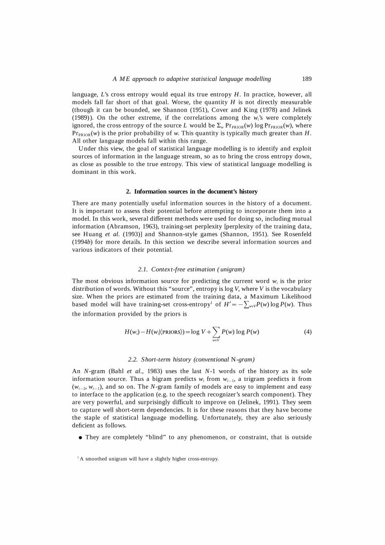
P (shares ~stock)
P (shares)
P (
shar
es)
1 2 3 4–10 11–25 26–50 51–100
101–200
201–500
501+
P (shares stock)
Figure 1. Probability of “SHARES” as a function of the distance (in words)from the last occurrence of “STOCK” in the same document. The middlehorizontal line is the unconditional probability. The top (bottom) line is theprobability of “SHARES” given that “STOCK” occurred (did not occur)before in the document).
of its occurrences. Then, for any candidate pair of words, we computed log crossproduct ratio, average mutual information (MI), and distance-based and count-basedco-occurrence statistics. The latter were used to draw graphs depicting detailed triggerrelations. Some illustrations are given in Figs 1 and 2. After using the program tomanually browse through many hundreds of trigger pairs, we were able to draw thefollowing general conclusions.
(1) Different trigger pairs display different behaviour, and hence should be modelleddifferently. More detailed modelling should be used when the expected return ishigher.
(2) Self triggers (i.e. triggers of the form (A→A)) are particularly powerful and robust.In fact, for more than two thirds of the words, the highest-MI trigger proved tobe the word itself. For 90% of the words, the self-trigger was among the top sixtriggers.
(3) Same-root triggers are also generally powerful, depending on the frequency of theirinflection.
(4) Most of the potential of triggers is concentrated in high-frequency words.(STOCK→BOND) is indeed much more useful than (BREST→LITOVSK).
(5) When the trigger and triggered words are from different domains of discourse, thetrigger pair actually shows some slight mutual information. The occurrence of aword like “STOCK” signifies that the document is probably concerned with financial

194 R. Rosenfeld
P (winter)
P (winter summer)
P (
win
ter)
0 1 2 3 4+
C (summer)
Figure 2. Probability of “WINTER” as a function of the number of times“SUMMER” occurred before it in the same document. Horizontal lines areas in Fig. 1.
issues, thus reducing the probability of words characteristic of other domains. Suchnegative triggers can in principle be exploited in much the same way as regular,“positive” triggers. However, the amount of information they provide is typicallyvery small.
2.6. Syntactic constraints
Syntactic constraints are varied. They can be expressed as yes/no decisions aboutgrammaticality, or, more cautiously, as scores, with very low scores assigned toungrammatical utterances.
The extraction of syntactic information would typically involve a parser. Un-fortunately, parsing of general English with reasonable coverage is not currentlyattainable. As an alternative, phrase parsing can be used. Another possibility is loosesemantic parsing (Ward, 1990, 1991), extracting syntactic-semantic information.
The information content of syntactic constraints is hard to measure quantitatively.But they are likely to be very beneficial. This is because this knowledge source seemscomplementary to the statistical knowledge sources we can currently tame. Many ofthe speech recognizer’s errors are easily identified as such by humans because theyviolate basic syntactic constraints.

195A ME approach to adaptive statistical language modelling
3. Combining information sources
Once the desired information sources are identified and the phenomena to be modelledare determined, one main issue still needs to be addressed. Given the part of thedocument processed so far (h), and a word w considered for the next position, thereare many different estimates of P(w|h). These estimates are derived from the differentknowledge sources. How does one combine them all to form one optimal estimate? Wediscuss existing solutions in this section, and propose a new one in the next.
3.1. Linear interpolation
Given k models {Pi(w|h)}i=1...k, we can combine them linearly with:
PCOMBINED(w|h) =def
]k
i=1
kiPi(w|h) (6)
where 0<kiΖ1 and ;ik i=1.
This method can be used both as a way of combining knowledge sources, and as away of smoothing (when one of the component models is very “flat”, such as a uniformdistribution). An Estimation–Maximization (EM) type algorithm (Dempster et al.,1977) is typically used to determine these weights. The result is a set of weights that isprovably optimal with regard to the data used for its optimization. See Jelinek andMercer (1980) for more details, and Rosenfeld (1994b) for further exposition.
Linear interpolation has very significant advantages, which make it the method ofchoice in many situations:
• Linear interpolation is extremely general. Any language model can be used as acomponent. In fact, once a common set of heldout data is selected for weightoptimization, the component models need no longer be maintained explicitly. Instead,they can be represented in terms of the probabilities they assign to the heldout data.Each model is represented as an array of probabilities. The EM algorithm simplylooks for a linear combination of these arrays that would minimize perplexity, andis completely unaware of their origin.
• Linear interpolation is easy to implement, experiment with, and analyse. We havecreated an interpolate program that takes any number of probability streams,and an optional bin-partitioning stream, and runs the EM algorithm to convergence(see Rosenfeld, 1994b: appendix B). We have used the program to experiment withmany different component models and bin-classification schemes. Some of our generalconclusions are as follows.(1) The exact value of the weights does not significantly affect perplexity. Weights
need only be specified to within >5% accuracy.(2) Very little heldout data (several hundred words per weight or less) are enough
to arrive at reasonable weights.• Linear interpolation cannot hurt. The interpolated model is guaranteed to be no
worse than any of its components. This is because each of the components can beviewed as a special case of the interpolation, with a weight of 1 for that componentand 0 for all others. Strictly speaking, this is only guaranteed for the heldout data,not for new data. But if the heldout data set is large enough and representative, the

196 R. Rosenfeld
T II. Perplexity reduction by linearly interpolating the trigram with atrigger model. See Rosenfeld and Huang (1992) for details
Test set Trigram PP Trigram+triggers PP Improvement
70KW (WSJ) 170 153 10%
result will carry over. So, if we suspect that a new knowledge source can contributeto our current model, the quickest way to test it would be to build a simple modelthat uses that source, and to interpolate it with our current one. If the new sourceis not useful, it will simply be assigned a very small weight by the EM algorithm(Jelinek, 1989).
Linear interpolation is so advantageous because it reconciliates the different in-formation sources in a straightforward and simple-minded way. But that simple-mindedness is also the source of its weaknesses:• Linearly interpolated models make suboptimal use of their components. The different
information sources are consulted “blindly”, without regard to their strengths andweaknesses in particular contexts. Their weights are optimized globally, not locally(the “bucketing” scheme is an attempt to remedy this situation piece-meal). Thusthe combined model does not make optimal use of the information at its disposal.
For example, in Section 2.4 we discussed Huang et al. (1993a), and reported ourconclusion that a significant amount of information exists in long-distance bigrams,up to distance 4. We have tried to incorporate this information by combining thesecomponents using linear interpolation. But the combined model improved perplexityover the conventional (distance 1) bigram by an insignificant amount (2%). In Section5 we will see how a similar information source can contribute significantly toperplexity reduction, provided a better method of combining evidence is employed.
As another, more detailed, example, in Rosenfeld and Huang (1992) we report onour early work on trigger models. We used a trigger utility measure, closely relatedto mutual information, to select some 620 000 triggers. We combined evidence frommultiple triggers using several variants of linear interpolation, then interpolated theresult with a conventional backoff trigram. An example result is in Table II. The10% reduction in perplexity, however gratifying, is well below the true potential ofthe triggers, as will be demonstrated in the following sections.• Linearly interpolated models are generally inconsistent with their components. Each
information source typically partitions the event space (h, w) and provides estimatesbased on the relative frequency of training data within each class of the partition.Therefore, within each of the component models, the estimates are consistent withthe marginals of the training data. But this reasonable measure of consistency is ingeneral violated by the interpolated model.
For example, a bigram model partitions the event space according to the last wordof the history. All histories that end in, say, “BANK” are associated with the sameestimate, PBIGRAM(w|h). That estimate is consistent with the portion of the trainingdata that ends in “BANK”, in the sense that, for every word w,

197A ME approach to adaptive statistical language modelling
]hvTRAINING-SETh ends in “BANK”
PBIGRAM(w|h)=C(, w) (7)
where C(, w) is the training-set count of the bigram (, w). However, whenthe bigram component is linearly interpolated with another component, based on adifferent partitioning of the data, the combined model depends on the assignedweights. These weights are in turn optimized globally, and are thus influenced by theother marginals and by other partitions. As a result, Equation (7) generally does nothold for the interpolated model.
3.2. Backoff
In the backoff method (Katz, 1987), the different information sources are ranked inorder of detail or specificity. At runtime, the most detailed model is consulted first. Ifit is found to contain enough information about the predicted word in the currentcontext, then that context is used exclusively to generate the estimate. Otherwise, thenext model in line is consulted. As in the previous case, backoff can be used both as away of combining information sources, and as a way of smoothing.
The backoff method does not actually reconcile multiple models. Instead, it choosesamong them. One problem with this approach is that it exhibits a discontinuity aroundthe point where the backoff decision is made. In spite of this problem, backing off issimple, compact, and often better than linear interpolation.
A problem common to both linear interpolation and backoff is that they give riseto systematic overestimation of some events. This problem was discussed and solvedin Rosenfeld and Huang (1992), and the solution used in a speech recognition systemin Chase et al. (1994).
4. The maximum entropy principle
In this section we discuss an alternative method of combining knowledge sources, whichis based on the Maximum Entropy approach advocated by E. T. Jaynes in the 1950’s(Jaynes, 1957). The Maximum Entropy principle was first applied to language modellingby DellaPietra et al. (1992).
In the methods described in the previous section, each knowledge source was usedseparately to construct a model, and the models were then combined. Under theMaximum Entropy approach, one does not construct separate models. Instead, onebuilds a single, combined model, which attempts to capture all the information providedby the various knowledge sources. Each such knowledge source gives rise to a set ofconstraints, to be imposed on the combined model. These constraints are typicallyexpressed in terms of marginal distributions, as in the example at the end of Section3.1. This solves the inconsistency problem discussed in that section.
The intersection of all the constraints, if not empty, contains a (typically infinite) setof probability functions, which are all consistent with the knowledge sources. Thesecond step in the Maximum Entropy approach is to choose, from among the functionsin that set, that function which has the highest entropy (i.e. the “flattest” function). Inother words, once the desired knowledge sources have been incorporated, no other
198 R. Rosenfeld
T III. The Event Space {(h, w)} is partitioned bythe bigram into equivalence classes (depicted here ascolumns). In each class, all histories end in the sameword
h ends in “THE” h ends in “OF” . . . . . .
· · · ·· · · ·· · · ·· · · ·· · · ·· · · ·
features of the data are assumed about the source. Instead, the “worst” (flattest) of theremaining possibilities is chosen.
Let us illustrate these ideas with a simple example.
4.1. An example
Assume we wish to estimate P(“BANK”|h), namely the probability of the word “BANK”given the document’s history. One estimate may be provided by a conventional bigram.The bigram would partition the event space (h, w) based on the last word of the history.The partition is depicted graphically in Table III. Each column is an equivalence classin this partition.
Consider one such equivalence class, say, the one where the history ends in “THE”.The bigram assigns the same probability estimate to all events in that class:
PBIGRAM(BANK|THE)=K{THE,BANK} (8)
That estimate is derived from the distribution of the training data in that class.Specifically, it is derived as:
K{THE,BANK} =def C(,)
C()(9)
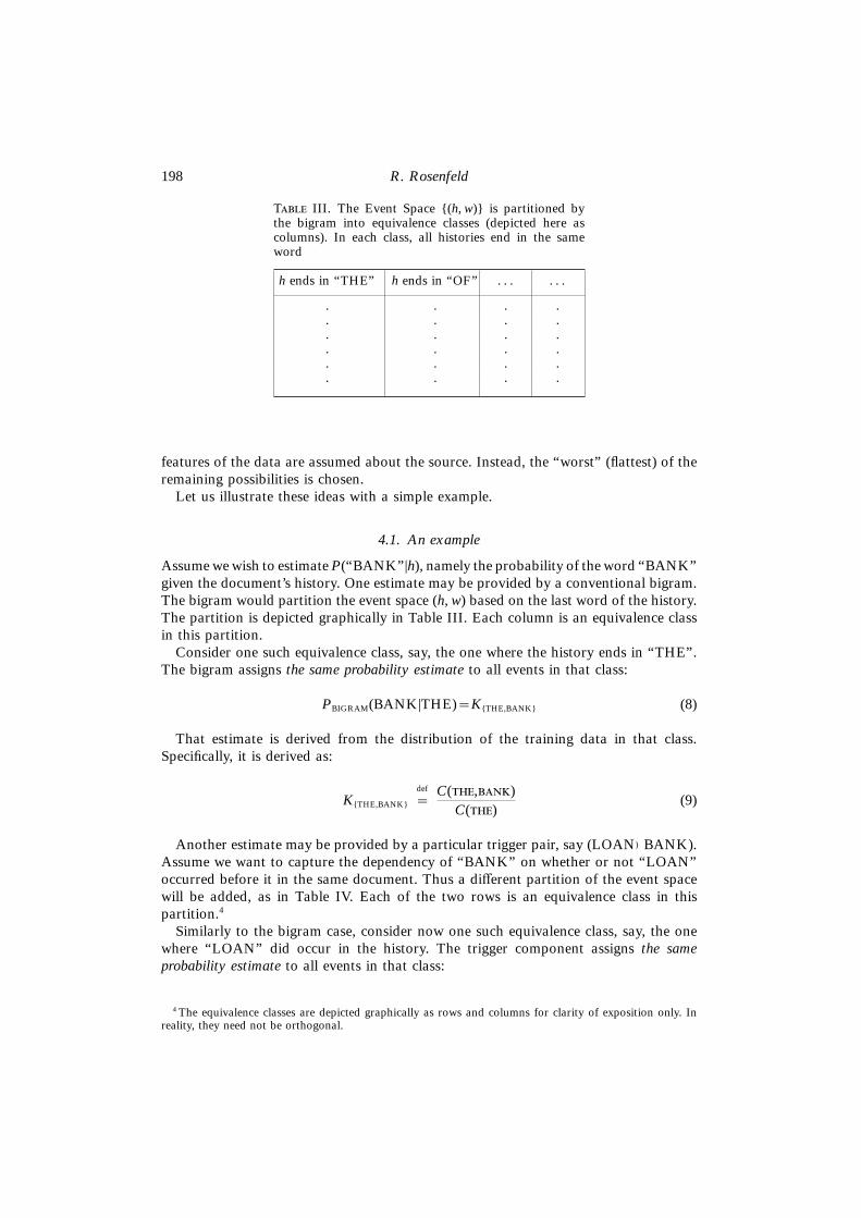
Another estimate may be provided by a particular trigger pair, say (LOAN)BANK).Assume we want to capture the dependency of “BANK” on whether or not “LOAN”occurred before it in the same document. Thus a different partition of the event spacewill be added, as in Table IV. Each of the two rows is an equivalence class in thispartition.4
Similarly to the bigram case, consider now one such equivalence class, say, the onewhere “LOAN” did occur in the history. The trigger component assigns the sameprobability estimate to all events in that class:
4 The equivalence classes are depicted graphically as rows and columns for clarity of exposition only. Inreality, they need not be orthogonal.
199A ME approach to adaptive statistical language modelling
T IV. The Event Space {(h, w)} is independently partitioned by thebinary trigger word “LOAN” into another set of equivalence classes(depicted here as rows)
h ends in “THE” h ends in “OF” . . . . . .
· · · ·LOANvh . . . . . . . . . . . . . . . . . . . .
· · · ·· · · ·
LOANvh . . . . . . . . . . . . . . . . . . . .· · · ·
PLOAN→BANK(BANK|LOANvh)=K{BANK,LOANvh} (10)
That estimate is derived from the distribution of the training data in that class.Specifically, it is derived as:
K{BANK,LOANvh} =def C(BANK,LOANvh)
C(LOANvh)(11)
Thus the bigram component assigns the same estimate to all events in the samecolumn, whereas the trigger component assigns the same estimate to all events in thesame row. These estimates are clearly mutually inconsistent. How can they be reconciled?
Linear interpolation solves this problem by averaging the two answers. The backoffmethod solves it by choosing one of them. The Maximum Entropy approach, on theother hand, does away with the inconsistency by relaxing the conditions imposed by thecomponent sources.
Consider the bigram. Under Maximum Entropy, we no longer insist that P(|h)always have the same value (K{THE,BANK}) whenever the history ends in “THE”. Instead,we acknowledge that the history may have other features that affect the probability of“BANK”. Rather, we only require that, in the combined estimate, P(|h) be equalto K{THE,BANK} on average in the training data. Equation (8) is replaced by
Eh ends in “THE”
[PCOMBINED(BANK|h)]=K{THE,BANK} (12)
where E stands for an expectation, or average. Note that the constraint expressed byEquation (12) is much weaker than that expressed by Equation (8). There are manydifferent functions PCOMBINED that would satisfy it. Only one degree of freedom wasremoved by imposing this new constraint, and many more remain.
Similarly, we require that PCOMBINED(|h) be equal to K{BANK,LOANvh} on averageover those histories that contain occurrences of “LOAN”:
E“LOAN”vh
[PCOMBINED(BANK|h)]=K{BANK,LOANvh} (13)
As in the bigram case, this constraint is much weaker than that imposed by Equation(10).
200 R. Rosenfeld
Given the tremendous number of degrees of freedom left in the model, it is easy tosee why the intersection of all such constraints would be non-empty. The next step inthe Maximum Entropy approach is to find, among all the functions in that intersection,the one with the highest entropy. The search is carried out implicitly, as will be describedin Section 4.3.
4.2. Information sources as constraint functions
Generalizing from the example above, we can view each information source as defininga subset (or many subsets) of the event space (h, w). For each subset, we impose aconstraint on the combined estimate to be derived: that it agrees on average with acertain statistic of the training data, defined over that subset. In the example above,the subsets were defined by a partition of the space, and the statistic was the marginaldistribution of the training data in each one of the equivalence classes. But this neednot be the case. We can define any subset S of the event space, and any desiredexpectation K, and impose the constraint:
](h,w)vS
[P(h, w)]=K (14)
The subset S can be specified by an index function, also called selector function, fs:
fs(h, w) =def
G10
if (h, w)vSotherwise
so Equation (14) becomes:
](h,w)
[P(h, w)fs(h, w)]=K (15)
This notation suggests further generalization. We need not restrict ourselves to indexfunctions. Any real-valued function f(h, w) can be used. We call f(h, w) a constraintfunction, and the associated K the desired expectation. Equation (15) now becomes:
ο f, Pπ=K (16)
This generalized constraint suggests a new interpretation: ο f, Pπ is the expectationof f(h, w) under the desired distribution P(h, w). We require P(h, w) to be such that theexpectation of some given functions { fi(h, w)}i=1,2,... match some desired values{Ki}i=1,2,..., respectively.
The generalizations introduced above are extremely important, because they meanthat any correlation, effect, or phenomenon that can be described in terms of statisticsof (h, w) can be readily incorporated into the Maximum Entropy model. All informationsources described in the previous section fall into this category, as do all otherinformation sources that can be described by an algorithm.
Following is a general description of the Maximum Entropy model and its solution.

201A ME approach to adaptive statistical language modelling
4.3. Maximum entropy and the generalized iterative scaling algorithm
The Maximum Entropy (ME) Principle (Jaynes, 1957; Kullback, 1959) can be statedas follows.
(1) Reformulate the different information sources as constraints to be satisfied by thetarget (combined) estimate.
(2) Among all probability distributions that satisfy these constraints, choose the onethat has the highest entropy.
Given a general event space {x}, to derive a combined probability function P(x),each constraint i is associated with a constraint function fi(x) and a desired expectationKi. The constraint is then written as:
EPfi =def
]x
P(x)fi(x)=Ki (17)
Given consistent constraints, a unique ME solution is guaranteed to exist, and to beof the form:
P(x)=\i
lfi(x)i (18)
where the li’s are some unknown constants, to be found. To search the exponentialfamily defined by Equation (18) for the li’s that will make P(x) satisfy all the constraints,an iterative algorithm, “Generalized Iterative Scaling” (GIS, Darroch & Ratcliff, 1972),exists, which is guaranteed to converge to the solution. GIS starts with some arbitraryl(0)
i values, which define the initial probability estimate:
P(0)(x) =def
\i
l(0)fi(x)i
Each iteration creates a new estimate, which is improved in the sense that it matchesthe constraints better than its predecessor. Each iteration (say j) consists of the followingsteps:
(1) Compute the expectations of all the fi’s under the current estimate function. Namely,
compute EP( j )fi =def
;x P( j)(x)fi(x).
(2) Compare the actual values (EP( j)fi’s) to the desired values (Ki’s), and update the li’saccording to the following formula:
l( j+1)i =l( j)
i ·Ki
EP( j)fi
(19)
(3) Define the next estimate function based on the new li’s:
202 R. Rosenfeld
P( j+1)(x) =def
\i
l( j+1)fi(x)i (20)
Iterating is continued until convergence or near-convergence.
4.4. Estimating conditional distributions
Generalized Iterative Scaling can be used to find the ME estimate of a simple (non-conditional) probability distribution over some event space. But in language modelling,we often need to estimate conditional probabilities of the form P(w|h). How shouldthis be done?
One simple way is to estimate the joint, P(h, w), from which the conditional, P(w|h),can be readily derived. This has been tried, with moderate success only, by Lau et al.(1993b). The likely reason is that the event space {(h, w)} is of size O(VL+1), where Vis the vocabulary size and L is the history length. For any reasonable values of V andL, this is a huge space, and no feasible amount of training data is sufficient to train amodel for it.
A better method was later proposed by Brown et al. (1994). Let P(h, w) be the desiredprobability estimate, and let P(h, w) be the empirical distribution of the training data.Let fi(h, w) be any constraint function, and let Ki be its desired expectation. Equation(17) can be rewritten as:
]h
P(h) ·]w
P(w|h) · fi(h, w)=Ki (21)
We now modify the constraint to be:
]h
P(h) ·]w
P(w|h) · fi(h, w)=Ki (22)
One possible interpretation of this modification is as follows. Instead of constrainingthe expectation of fi(h, w) with regard to P(h, w), we constrain its expectation withregard to a different probability distribution, say Q(h, w), whose conditional Q(w|h) isthe same as that of P, but whose marginal Q(h) is the same as that of P. To betterunderstand the effect of this change, define H as the set of all possible histories h, anddefine Hfi as the partition of H induced by fi. Then the modification is equivalent toassuming that, for every constraint fi, P(Hfi)=P(Hfi). Since typically Hfi is a very smallset, the assumption is reasonable. It has several significant benefits as follows.
(1) Although Q(w|h)=P(w|h), modelling Q(h, w) is much more feasible than modellingP(h, w), since Q(h, w)=0 for all but a minute fraction of the h’s.
(2) When applying the Generalized Iterative Scaling algorithm, we no longer need tosum over all possible histories (a very large space). Instead, we only sum over thehistories that occur in the training data.
(3) The unique ME solution that satisfies equations like Equation (22) can be shownto also be the Maximum Likelihood (ML) solution, namely that function which,among the exponential family defined by the constraints, has the maximum likelihood

203A ME approach to adaptive statistical language modelling
of generating the training data. The identity of the ML and ME solutions, apartfrom being aesthetically pleasing, is extremely useful when estimating the conditionalP(w|h). It means that hillclimbing methods can be used in conjunction withGeneralized Iterative Scaling to speed up the search. Since the likelihood objectivefunction is convex, hillclimbing will not get stuck in local minima.
4.5. Maximum entropy and minimum discrimination information
The principle of Maximum Entropy can be viewed as a special case of the MinimumDiscrimination Information (MDI) principle. Let P0(x) be a prior probability function,and let {Qa(x)}a be a family of probability functions, where a varies over some set. Asin the case of Maximum Entropy, {Qa(x)}a might be defined by an intersection ofconstraints. One might wish to find the function Q0(x) in that family which is closestto the prior P0(x):
Q0(x) =def
arg mina
D(Qa, P0) (23)
where the non-symmetric distance measure, D(Q, P), is the Kullback–Liebler distance,also known as discrimination information or asymmetric divergence (Kullback, 1959):
D(Q(x), P(x)) =def
]x
Q(x) logQ(x)P(x)
(24)
In the special case when P0(x) is the uniform distribution, Q0(x) as defined byEquation (23) is also the Maximum Entropy solution, namely the function with thehighest entropy in the family {Qa(x)}a. We see thus that ME is a special case of MDI,where the distance is measured to the uniform distribution.
In a precursor to this work, DellaPietra et al. (1992) used the history of a documentto construct a unigram. The latter was used to constrain the marginals of a bigram.The static bigram was used as the prior, and the MDI solution was sought among thefamily defined by the constrained marginals.
4.6. Assessing the maximum entropy approach
The ME principle and the Generalized Iterative Scaling algorithm have several importantadvantages as follows.
(1) The ME principle is simple and intuitively appealing. It imposes all of the constituentconstraints, but assumes nothing else. For the special case of constraints derivedfrom marginal probabilities, it is equivalent to assuming a lack of higher-orderinteractions (Good, 1963).
(2) ME is extremely general. Any probability estimate of any subset of the event spacecan be used, including estimates that were not derived from the data or that areinconsistent with it. Many other knowledge sources can be incorporated, such asdistance-dependent correlations and complicated higher-order effects. Note thatconstraints need not be independent of nor uncorrelated with each other.
(3) The information captured by existing language models can be absorbed into the

204 R. Rosenfeld
ME model. Later on in this document we will show how this is done for theconventional N-gram model.
(4) Generalized Iterative Scaling lends itself to incremental adaptation. New constraintscan be added at any time. Old constraints can be maintained or else allowed torelax.
(5) A unique ME solution is guaranteed to exist for consistent constraints. TheGeneralized Iterative Scaling algorithm is guaranteed to converge to it.
This approach also has the following weaknesses.
(1) Generalized Iterative Scaling is computationally very expensive [for more on thisproblem, and on methods for coping with it, see Rosenfeld (1994b): section 5.7].
(2) While the algorithm is guaranteed to converge, we do not have a theoretical boundon its convergence rate (for all systems we tried, convergence was achieved within10–20 iterations).
(3) It is sometimes useful to impose constraints that are not satisfied by the trainingdata. For example, we may choose to use Good–Turing discounting (Good, 1953)(as we have indeed done in this work), or else the constraints may be derived fromother data, or be externally imposed. Under these circumstances, equivalencewith the Maximum Likelihood solution no longer exists. More importantly, theconstraints may no longer be consistent, and the theoretical results guaranteeingexistence, uniqueness and convergence may not hold.
5. Using maximum entropy in language modelling
In this section, we describe how the Maximum Entropy framework was used to createa language model which tightly integrates varied knowledge sources.
5.1. Distance-1 N-grams
5.1.1. Conventional formulationIn the conventional formulation of standard N-grams, the usual unigram, bigram andtrigram Maximum Likelihood estimates are replaced by unigram, bigram and trigramconstraints conveying the same information. Specifically, the constraint function forthe unigram w1 is:
fw1(h, w)=G10
if w=w1
otherwise(25)
The desired value, Kw1, is set to E[ fw1], the empirical expectation of fw1, i.e. its expectationin the training data:
E[ fw1] =def 1
N ](h,w)vTRAINING
fw1(h, w) (26)

205A ME approach to adaptive statistical language modelling
and the associated constraint is:
]h
P(h)]w
P(w|h)fw1(h, w)=E[ fw1] (27)
(As before, P( ) denotes the empirical distribution.) Similarly, the constraint functionfor the bigram {w1, w2} is:
f{w1,w2}(h, w)=G10
if h ends in w1 and w=w2
otherwise(28)
and its associated constraint is:
]h
P(h)]w
P(w|h)f{w1,w2}(h, w)=E[ f{w1,w2}]. (29)
Finally, the constraint function for the trigram {w1, w2, w3} is:
f{w1,w2,w3}(h, w)=G10
if h ends in (w1, w2) and w=w3
otherwise(30)
and its associated constraint is:
]h
P(h)]w
P(w|h)f{w1,w2,w3}(h, w)=E[ f{w1,w2,w3}] (31)
5.1.2. Complemented N-gram formulation
Each constraint in an ME model induces a subset of the event space {(h, w)}. One canmodify the N-gram constraints by modifying their respective subsets. In particular, thefollowing set subtraction operations can be performed.
(1) Modify each bigram constraint to exclude all events (h, w) that are part of anexisting trigram constraint (call these “complemented bigrams”).
(2) Modify each unigram constraint to exclude all events (h, w) that are part of anexisting bigram or trigram constraint (call these “complemented unigrams”).
These changes are not merely notational—the resulting model differs from the originalin significant ways. Neither are they applicable to ME models only. In fact, whenapplied to a conventional Backoff model, they yielded a modest reduction in perplexity.This is because at runtime, backoff conditions are better matched by the “complemented”events. Recently, Kneser and Ney (1995) used a similar observation to motivate theirown modification to the backoff scheme, with similar results.
For the purpose of the ME model, though, the most important aspect of complemented
206 R. Rosenfeld
N-grams is that their associated events do not overlap. Thus only one such constraintis active for any training datapoint (instead of up to three). This in turn results in fasterconvergence of the Generalized Iterative Scaling algorithm (Rosenfeld, 1994b: p. 53).For this reason we have chosen to use the complemented N-gram formulation in thiswork.
5.2. Triggers
5.2.1. Incorporating triggers into METo formulate a (binary) trigger pair A)B as a constraint, define the constraint functionfA)B as:
fA→B(h, w)=G10
if Avh, w=Botherwise
(32)
Set KA)B to E[ fA)B], the empirical expectation of fA)B (i.e. its expectation in thetraining data). Now impose on the desired probability estimate P(h, w) the constraint:
]h
P(h)]w
P(w|h)fA)B(h, w)=E[ fA)B] (33)
5.2.2. Selecting trigger pairs
In Section 2.5.2, we discussed the use of mutual information as a measure of the utilityof a trigger pair. Given the candidate trigger pair (BUENOS→AIRES), this proposedmeasure would be:
I(BUENOS0: AIRES)=P(BUENOS0, AIRES) logP(AIRES|BUENOS0)
P(AIRES)
+P(BUENOS0, AIRES) logP(AIRES|BUENOS0)
P(AIRES)
+P(BUENOS0, AIRES) logP(AIRES|BUENOS0)
P(AIRES)
+P(BUENOS0, AIRES) logP(AIRES|BUENOS0)
P(AIRES)(34)
This measure is likely to result in a high utility score in this case. But is this triggerpair really that useful? Triggers are used in addition to N-grams. Therefore, triggerpairs are only useful to the extent that the information they provide supplements theinformation already provided by N-grams. In the example above, “AIRES” is almostalways predicted by “BUENOS”, using a bigram constraint.
One possible fix is to modify the mutual information measure, so as to factor out

207A ME approach to adaptive statistical language modelling
T V. The best triggers “A” for some given words “B”, in descending order, as measured byMI(A0–3g: B)
HARVEST ⇐ CROP HARVEST CORN SOYBEAN SOYBEANS AGRICULTURE GRAINDROUGHT GRAINS BUSHELS
HARVESTING⇐CROP HARVEST FORESTS FARMERS HARVESTING TIMBER TREESLOGGING ACRES FOREST
HASHEMI ⇐ IRAN IRANIAN TEHRAN IRAN’S IRANIANS LEBANON AYATOLLAHHOSTAGES KHOMEINI ISRAELI HOSTAGE SHIITE ISLAMIC IRAQ PERSIAN TER-RORISM LEBANESE ARMS ISRAEL TERRORIST
HASTINGS ⇐ HASTINGS IMPEACHMENT ACQUITTED JUDGE TRIAL DISTRICTFLORIDA
HATE ⇐ HATE MY YOU HER MAN ME I LOVE
HAVANA ⇐ CUBAN CUBA CASTRO HAVANA FIDEL CASTRO’S CUBA’S CUBANSCOMMUNIST MIAMI REVOLUTION
triggering effects that fall within the range of the N-grams. Let h=wi−11 . Recall that
A0 =def
{Avwi−11 }
Then, in the context of trigram constraints, instead of using MI(A0: B) we can useMI(A0-3g: B), where:
A0-3g =def
{Avwi−31 }
We will designate this measure with MI-3g.Using the WSJ occurrence file described in Section 2.5.2, the 400 million possible
(ordered) trigger pairs of the WSJ’s 20 000 word vocabulary were filtered. As a firststep, only word pairs that co-occurred in at least nine documents were maintained.This resulted in some 25 million (unordered) pairs. Next, MI(A0-3g: B) was computedfor all these pairs. Only pairs that had at least 1 milibit (0·001 bit) of average mutualinformation were kept. This resulted in 1·4 million ordered trigger pairs, which werefurther sorted by MI-3g, separately for each B. A random sample is shown in Table V.A larger sample is provided in Rosenfeld (1994b: appendix C).
Browsing the complete list, several conclusions could be drawn as follows.
(1) Self-triggers, namely words that trigger themselves (A→A) are usually very goodtrigger pairs. In fact, in 68% of the cases, the best predictor for a word is the worditself. In 90% of the cases, the self-trigger is among the top six predictors.
(2) Words based on the same stem are also good predictors.(3) In general, there is great similarity between same-stem words:
• The strongest association is between nouns and their possessive, both for triggers(i.e. B⇐. . . XYZ, . . . XYZ’S . . .) and for triggered words (i.e. the predictor setsof XYZ and XYZ’S are very similar).
• Next is the association between nouns and their plurals.

208 R. Rosenfeld
• Next is adjectivization (IRAN-IAN, ISRAEL-I).
(4) Even when predictor sets are very similar, there is still a preference to self-triggers(i.e. οXYZπ predictor-set is biased towards οXYZπ, οXYZπS predictor-set is biasedtowards οXYZπS, οXYZπ’S predictor-set is biased towards οXYZπ’S).
(5) There is preference to more frequent words, as can be expected from the mutualinformation measure.
The MI-3g measure is still not optimal. Consider the sentence:
“The district attorney’s office launched an investigation into loansmade by several well connected banks.”
The MI-3g measure may suggest that (ATTORNEY→INVESTIGATION) is a goodpair. And indeed, a model incorporating that pair may use “ATTORNEY” to trigger“INVESTIGATION” in the sentence above, raising its probability above the defaultvalue for the rest of the document. But when “INVESTIGATION” actually occurs, itis preceded by “LAUNCHED AN”, which allows the trigram component to predict itwith a much higher probability. Raising the probability of “INVESTIGATION” incurssome cost, which is never justified in this example. This happens because MI-3g stillmeasures “simple” mutual information, and not the excess mutual information beyondwhat is already supplied by the N-grams.
Similarly, trigger pairs affect each others’ usefulness. The utility of the trigger pairA1→B is diminished by the presence of the pair A2→B, if the information they providehas some overlap. Also, the utility of a trigger pair depends on the way it will be usedin the model. MI-3g fails to consider these factors as well.
For an optimal measure of the utility of a trigger pair, a procedure like the followingcould be used:
(1) Train an ME model based on N-grams alone.(2) For every candidate trigger pair (A→B), train a special instance of the base model
that incorporates that pair (and that pair only).(3) Compute the excess information provided by each pair by comparing the entropy
of predicting B with and without it.(4) For every B, choose the one trigger pair that maximizes the excess information.(5) Incorporate the new trigger pairs (one for each B in the vocabulary) into the base
model, and repeat from step 2.For a task as large as the WSJ (40 million words of training data, millions of constraints),this approach is clearly infeasible. But in much smaller tasks it could be employed (see,for example, Ratnaparkhi & Roukos, 1994).
5.2.3. A simple ME system
The difficulty in measuring the true utility of individual triggers means that, in general,one cannot directly compute how much information will be added to the system, andhence by how much entropy will be reduced. However, under special circumstances,this may still be possible. Consider the case where only unigram constraints are present,and only a single trigger is provided for each word in the vocabulary (one “A” foreach “B”). Because there is no “crosstalk” between the N-gram constraints and thetrigger constraints (nor among the trigger constraints themselves), it should be possible

209A ME approach to adaptive statistical language modelling
to calculate in advance the reduction in perplexity due to the introduction of thetriggers.
To verify the theoretical arguments (as well as to test the code), the followingexperiments were conducted on the 38 million words of the WSJ corpus languagetraining data (vocabulary=19 981, see Appendix A). First, an ME model incorporatingonly the unigram constraints was created. Its training-set perplexity (PP) was 962—exactly as calculated from simple Maximum Likelihood estimates. Next, for each word“B” in the vocabulary, the best predictor “A” (as measured by standard mutualinformation) was chosen. The 19 981 trigger pairs had a total mutual information of0·37988 bits. Based on the argument above, the training-set perplexity of the modelafter incorporating these triggers should be:
962×2−0·37988≈739
The triggers were then added to the model, and the Generalized Iterative Scalingalgorithm was run. It produced the following output.
I T-PP I
1 19981·02 1919·6 90·4%3 999·5 47·9%4 821·5 17·8%5 772.5 6·0%6 755·0 2·3%7 747.2 1·0%8 743·1 0·5%9 740·8 0·3%
10 739·4 0·2%
In complete agreement with the theoretical prediction.
5.3. A model combining N-grams and triggers
As a first major test of the applicability of the ME approach, ME models wereconstructed which incorporated both N-gram and trigger constraints. One experimentwas run with the best three triggers for each word (as judged by the MI-3g criterion),and another with the best six triggers per word.
In both N-gram and trigger constraints (as in all other constraints incorporatedlater), the desired value of each constraint (the right-hand side of Equations 27, 29, 31or 33) was replaced by its Good–Turing discounted value, since the latter is a betterestimate of the true expectation of that constraint in new data.5
5 Note that this modification invalidates the equivalence with the Maximum Likelihood solution discussedin Section 4.4. Furthermore, since the constraints no longer match the marginals of the training data, theyare not guaranteed to be consistent, and hence a solution is not guaranteed to exist. Nevertheless, ourintuition was that the large number of remaining degrees of freedom will practically guarantee a solution,and indeed this has always proven to be the case.

210 R. Rosenfeld
T VI. Maximum Entropy models incorporating N-gram and trigger constraints
Vocabulary Top 20 000 words of WSJ corpusTraining set 5MW (WSJ)Test set 325KW (WSJ)Trigram perplexity (baseline) 173 173ME experiment “top 3” “top 6”ME constraints:
unigrams 18 400 18 400bigrams 240 000 240 000trigrams 414 000 414 000triggers 36 000 65 000
ME perplexity 134 130perplexity reduction 23% 25%
0·75 · ME+0·25 · trigram perplexity 129 127perplexity reduction 25% 27%
A conventional backoff trigram model was used as a baseline. The Maximum Entropymodels were also linearly interpolated with the conventional trigram, using a weightof 0·75 for the ME model and 0·25 for the trigram. 325 000 words of new data wereused for testing.6 Results are summarized in Table VI.
Interpolation with the trigram model was done in order to test whether the MEmodel fully retained all the information provided by the N-grams, or whether part of itwas somehow lost when trying to incorporate the trigger information. Since interpolationreduced perplexity by only 2%, we conclude that almost all the N-gram informationwas retained by the integrated ME model. This illustrates the ability of the MEframework to successfully accommodate multiple knowledge sources.
Similarly, there was little improvement in using six triggers per word vs. three triggersper word. This could be because little information was left after three triggers thatcould be exploited by trigger pairs. More likely it is a consequence of the suboptimalmethod we used for selecting triggers (see Section 5.2.2). Many “A” triggers for thesame word “B” are highly correlated, which means that much of the information theyprovide overlaps. Unfortunately, the MI-3g measure discussed in Section 5.2.2 fails toaccount for this overlap.
The baseline trigram model used in this and all other experiments reported here wasa “compact” backoff model: all trigrams occurring only once in the training set wereignored. This modification, which is the standard in the ARPA community, results invery slight degradation in perplexity (1% in this case), but realizes significant savingsin memory requirements. All ME models describe here also discarded this information.
5.4. Class triggers
5.4.1. MotivationIn Section 5.2.2 we mentioned that strong triggering relations exist among differentinflections of the same stem, similar to the triggering relation a word has with itself. It
6 We used a large test set to ensure the statistical significance of the results. At this size, perplexity of halfthe data set, randomly selected, is within >1% of the perplexity of the whole set.
211A ME approach to adaptive statistical language modelling
is reasonable to hypothesize that the triggering relationship is really among the stems,not the inflections. This is further supported by our intuition (and observation) thattriggers capture semantic correlations. One might assume, for example, that the stem“LOAN” triggers the stem “BANK”. This relationship will hopefully capture, in aunified way, the affect that the occurrence of any of “LOAN”, “LOANS”, “LOAN’S”,and “LOANED” might have on the probability of any of “BANK”, “BANKS” and“BANKING” occurring next.
It should be noted that class triggers are not merely a notational shorthand. Even ifone wrote down all possible combinations of word pairs from the above two lists, theresult would not be the same as in using the single, class-based trigger. This is because,in a class trigger, the training data for all such word-pairs is clustered together. Whichsystem is better is an empirical question. It depends on whether these words do indeedbehave similarly with regard to long-distance prediction, which can only be decided bylooking at the data.
5.4.2. ME constraints for class trigger
Let AA =def
{A1, A2, . . . An} be some subset of the vocabulary, and let
BB =def
{B1, B2, . . . Bn} be another subset. The ME constraint function for the classtrigger (AA⇒BB) is:
fAA)BB(h, w)=G10
if (&A, AvAA, Avh)§wvBB
otherwise(35)
Set KAA)BB to E[ fAA)BB], the empirical expectation of fAA)BB. Now impose on the desiredprobability estimate P(h, w) the constraint:
]h
P(h)]w
P(w|h)fAA)BB(h, w)=E[ fAA)BB] (36)
5.4.3. Clustering words for class triggers
Writing the ME constraints for class triggers is straightforward. The hard problem isfinding useful classes. This is reminiscent of the case of class-based N-grams. Indeed,one could use any of the general methods discussed in Section 2.3: clustering bylinguistic knowledge, clustering by domain knowledge, or data driven clustering.
To estimate the potential of class triggers, we chose to use the first of these methods.The choice was based on the strong conviction that some stem-based clustering iscertainly “correct”. This conviction was further supported by the observations madein Section 5.2.2, after browsing the “best-predictors” list.
Using the “morphe” program, developed at Carnegie Mellon,7 each word in thevocabulary was mapped to one or more stems. That mapping was then reversed tocreate word clusters. The >20 000 words formed 13 171 clusters, 8714 of which were
7 We are grateful to David Evans and Steve Henderson for their generosity in providing us with this tool.

212 R. Rosenfeld
T VII. A randomly selected set of examples of stem-based clustering, using morphologicalanalysis provided by the “morphe” program
[ACCRUAL] : ACCRUAL[ACCRUE] : ACCRUE, ACCRUED, ACCRUING[ACCUMULATE] : ACCUMULATE, ACCUMULATED, ACCUMULATING[ACCUMULATION] : ACCUMULATION[ACCURACY] : ACCURACY[ACCURATE] : ACCURATE, ACCURATELY[ACCURAY] : ACCURAY[ACCUSATION] : ACCUSATION, ACCUSATIONS[ACCUSE] : ACCUSE, ACCUSED, ACCUSES, ACCUSING[ACCUSTOM] : ACCUSTOMED[ACCUTANE] : ACCUTANE[ACE] : ACE[ACHIEVE] : ACHIEVE, ACHIEVED, ACHIEVES, ACHIEVING[ACHIEVEMENT] : ACHIEVEMENT, ACHIEVEMENTS[ACID] : ACID
T VIII. Word self-triggers vs. class self-triggers, in the presence of unigram constraints.Stem-based clustering does not help much
Vocabulary Top 20 000 words of WSJ corpusTraining set 300KW (WSJ)Test set 325KW (WSJ)Unigram perplexity 903Model Word self-triggers Class self-triggersME constraints:
unigrams 9017 9017word self-triggers 2658 —class self-triggers — 2409
Training-set perplexity 745 740Test-set perplexity 888 870
singletons. Some words belonged to more than one cluster. A randomly selected sampleis shown in Table VII.
Next, two ME models were trained. The first included all “word self-triggers”, onefor each word in the vocabulary. The second included all “class self-triggers” ( fAA)AA),one for each cluster AA. A threshold of three same-document occurrences was usedfor both types of triggers. Both models also included all the unigram constraints, witha threshold of two global occurrences. The use of only unigram constraints facilitatedthe quick estimation of the amount of information in the triggers, as was discussed inSection 5.2.3. Both models were trained on the same 300 000 words of WSJ text.Results are summarized in Table VIII.
Surprisingly, stem-based clustering resulted in only a 2% improvement in test–setperplexity in this context. One possible reason is the small amount of training data,which may not be sufficient to capture long-distance correlations among the lesscommon members of the clusters. The experiment was therefore repeated, this time

213A ME approach to adaptive statistical language modelling
T IX. Word self-triggers vs. class self-triggers, using more training data than in the previousexperiment (Table VIII). Results are even more disappointing
Vocabulary Top 20 000 words of WSJ corpusTraining set 5MW (WSJ)Test set 325KW (WSJ)Unigram perplexity 948Model Word self-triggers Class self-triggersME constraints:
unigrams 19 490 19 490word self-triggers 10 735 —class self-triggers — 12 298
Training-set perplexity 735 733Test-set perplexity 756 758
training on 5 million words. Results are summarized in Table IX, and are even moredisappointing. The class-based model is actually slightly worse than the word-basedone (though the difference appears insignificant).
Why did stem-based clustering fail to improve perplexity? We did not find a satisfactoryexplanation. One possibility is as follows. Class triggers are allegedly superior to wordtriggers in that they also capture within-word, cross-word effects, such as the effect“ACCUSE” has on “ACCUSED”. But stem-based clusters often consist of one commonword and several much less frequent variants. In these cases, all within-cluster cross-word effects include rare words, which means their impact is very small (recall that atrigger pair’s utility depends on the frequency of both its words).
5.5. Long distance N-grams
In Section 2.4 we showed that there is quite a bit of information in bigrams of distance2, 3 and 4. But in Section 3.1, we reported that we were unable to benefit from thisinformation using linear interpolation. With the Maximum Entropy approach, however,it might be possible to better integrate that knowledge.
5.5.1. Long distance N-gram constraints
Long distance N-gram constraints are incorporated into the ME formalism in muchthe same way as the conventional (distance 1) N-grams. For example, the constraintfunction for distance-j bigram {w1, w2} is
f [j]{w1,w2}(h, w)=G1
0if h=wi−1
1 , wi−j=w1 and w=w2
otherwise(37)
and its associated constraint is
]h
P(h)]w
P(w|h)f [j]{w1,w2}(h, w)=E[f [j]
{w1,w2}]. (38)
where E[ f [j]{w1,w2}] is the expectation of f [ j]
{w1,w2} in the training data:

214 R. Rosenfeld
T X. A Maximum Entropy model incorporating N-gram, distance-2 N-gram and triggerconstraints. The 38MW system used far fewer parameters than the baseline, since it employedhigh N-gram thresholds to reduce training time
Vocabulary Top 20 000 words of WSJ corpusTest set 325KWTraining set 1MW 5MW 38MW∗Trigram perplexity (baseline) 269 173 105ME constraints:
unigrams 13 130 18 421 19 771bigrams 65 397 240 256 327 055trigrams 79 571 411 646 427 560distance-2 bigrams 67 186 280 962 651 418distance-2 trigrams 65 600 363 095 794 818word triggers (max 3/word) 20 209 35 052 43 066
Training time (alpha-days) <1 12 >200Test-set perplexity 203 123 86
perplexity reduction 24% 29% 18%
E[f [ j]{w1,w2} =
def 1N ]
(h,w)vTRAINING
f [ j]{w1,w2}(h, w) (39)
Similarly for the trigram constraints, and similarly for “complemented N-grams”(Section 5.1.2).
5.6. Adding distance-2 N-grams to the model
The model described in Section 5.3 was augmented to include distance-2 bigrams andtrigrams. Three different systems were trained, on different amounts of training data:1 million words, 5 million words, and 38 million words (the entire WSJ corpus). Thesystems and their performance are summarized in Table X. The trigram model used asbaseline was described in Section 5.3. Training time is reported in “alpha-days” whichis the amount of computation done by a DEC/Alpha 3000/500 workstation in 24 h.
The 38MW system was different than the others, in that it employed high thresholds(cutoffs) on the N-gram constraints: distance-1 bigrams and trigrams were includedonly if they occurred at least nine times in the training data. Distance-2 bigrams andtrigrams were included only if they occurred at least five times in the training data.This was done to reduce the computational load, which was quite severe for a systemthis size. The cutoffs used for the conventional N-grams were higher than those appliedto the distance-2 N-grams because it was anticipated that the information lost fromthe former knowledge source will be re-introduced later, at least partially, by in-terpolation with the conventional trigram model. The actual values of the cutoffs werechosen so as to make it possible to finish the computation in 2–3 weeks.
As can be observed, the Maximum Entropy model is significantly better than thetrigram model. Its relative advantage seems greater with more training data. With thelarge (38MW) system, practical consideration required imposing high cutoffs on theME model, and yet its perplexity is still significantly better than that of the baseline.This is particularly notable because the ME model uses only one third the number ofparameters used by the trigram model (2·26 million vs. 6·72 million).
215A ME approach to adaptive statistical language modelling
T XI. Perplexity of Maximum Entropy models for various subsets of the information sourcesused in Table X. With 1MW of training data, information provided by distance-2 N-grams islargely overlapped by that provided by triggers
Vocabulary Top 20 000 words of WSJ corpusTraining set 1MWTest set 325KW
Perplexity % changeTrigram (baseline) 269 —ME models:
dist.-1 N-grams+dist.-2 N-grams 249 −8%dist.-1 N-grams+word triggers 208 −23%dist.-1 N-grams+dist.-2 N-grams+word triggers 203 −24%
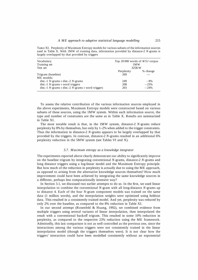
To assess the relative contribution of the various information sources employed inthe above experiments, Maximum Entropy models were constructed based on varioussubsets of these sources, using the 1MW system. Within each information source, thetype and number of constraints are the same as in Table X. Results are summarizedin Table XI.
The most notable result is that, in the 1MW system, distance-2 N-grams reduceperplexity by 8% by themselves, but only by 1–2% when added to the trigger constraints.Thus the information in distance-2 N-grams appears to be largely overlapped by thatprovided by the triggers. In contrast, distance-2 N-grams resulted in an additional 6%perplexity reduction in the 5MW system (see Tables VI and X).
5.7. Maximum entropy as a knowledge integrator
The experiments reported above clearly demonstrate our ability to significantly improveon the baseline trigram by integrating conventional N-grams, distance-2 N-grams andlong distance triggers using a log-linear model and the Maximum Entropy principle.But how much of the reduction in perplexity is actually due to using the ME approach,as opposed to arising from the alternative knowledge sources themselves? How muchimprovement could have been achieved by integrating the same knowledge sources ina different, perhaps less computationally intensive way?
In Section 3.1, we discussed two earlier attempts to do so. In the first, we used linearinterpolation to combine the conventional N-gram with all long-distance N-grams upto distance 4. Each of the four N-gram component models was trained on the samedata (1 million words), and the interpolation weights were optimized using heldoutdata. This resulted in a consistently trained model. And yet, perplexity was reduced byonly 2% over the baseline, as compared to the 8% reduction in Table XI.
In our second attempt (Rosenfeld & Huang, 1992), we combined evidence frommultiple triggers using several variants of linear interpolation, then interpolated theresult with a conventional backoff trigram. This resulted in some 10% reduction inperplexity, as compared to the respective 23% reduction using the ME framework.Admittedly, this last comparison is not as well controlled as the previous one, since theinteractions among the various triggers were not consistently trained in the linearinterpolation model (though the triggers themselves were). It is not clear how thetriggers’ interaction could have been modelled consistently without an exponential

216 R. Rosenfeld
growth in the number of parameters. In any case, this only serves to highlight one ofthe biggest advantages of the ME method: that it facilitates the consistent andstraightforward incorporation of diverse knowledge sources.
6. Adaptation in language modelling
6.1. Adaptation vs. long distance modelling
This work grew out of a desire to improve on the conventional trigram language model,by extracting information from the document’s history. This approach is often termed“long-distance modelling”. The trigger pair was chosen as the basic information bearingelement for that purpose.
But triggers can be also viewed as vehicles of adaptation. As the topic of discoursebecomes known, triggers capture and convey the semantic content of the document,and adjust the language model so that it better anticipates words that are more likelyin that domain. Thus the models discussed so far can be considered adaptive as well.
This duality of long-distance modelling and adaptive modelling is quite strong. Thereis no clear distinction between the two. In one extreme, a trigger model based on thehistory of the current document can be viewed as a static (non-adaptive) probabilityfunction whose domain is the entire document history. In another extreme, a trigrammodel can be viewed as a bigram which is adapted at every step, based on thepenultimate word of the history.
Fortunately, this type of distinction is not very important. More meaningful isclassification based on the nature of the language source, and the relationship betweenthe training and test data. In this section we propose such classification, and study theadaptive capabilities of Maximum Entropy and other modelling techniques.
6.2. Three paradigms of adaptation
The adaptation discussed so far was the kind we call within-domain adaptation. In thisparadigm, a heterogeneous language source (such as WSJ) is treated as a complexproduct of multiple domains-of-discourse (“sublanguages”). The goal is then to producea continuously modified model that tracks sublanguage mixtures, sublanguage shifts,style shifts, etc.
In contrast, a cross-domain adaptation paradigm is one in which the test data comesfrom a source to which the language model has never been exposed. The most salientaspect of this case is the large number of out-of-vocabulary words in the test data, aswell as the high proportion of new bigrams and trigrams.
Cross-domain adaptation is most important in cases where no data from the testdomain is available for training the system. But in practice this rarely happens. Morelikely, a limited amount of training data can be obtained. Thus a hybrid paradigm,limited-data domain adaptation, might be the most important one for real-worldapplications.
6.3. Within-domain adaptation
Maximum Entropy models are naturally suited for within-domain adaptation.8 This isbecause constraints are typically derived from the training data. The ME model
8 Although they can be modified for cross-domain adaptation as well. See next subsection.

217A ME approach to adaptive statistical language modelling
integrates the constraints, making the assumption that the same phenomena will holdin the test data as well.
But this last assumption is also a limitation. Of all the triggers selected by the mutualinformation measure, self-triggers were found to be particularly prevalent and strong(see Section 5.2.2). This was true for very common, as well as moderately commonwords. It is reasonable to assume that it also holds for rare words. Unfortunately,Maximum Entropy triggers as described above can only capture self-correlations thatare well represented in the training data. As long as the amount of training data isfinite, self correlation among rare words is not likely to exceed the threshold. To capturethese effects, the ME model was supplemented with a “rare words only” unigram cache,to be described in the next subsection.
Another source of adaptive information is self-correlations among word sequences.In principle, these can be captured by appropriate constraint functions, describingtrigger relations among word sequences. But our implementation of triggers was limitedto single word triggers. To capture these correlations, conditional bigram and trigramcaches were added, to be described subsequently.
N-gram caches were first reported by Kuhn (1988) and Kupiec (1989). Kuhn andDe Mori (1990, 1992) employed a POS-based bigram cache to improve the performanceof their static bigram. Jelinek et al. (1991) incorporated a trigram cache into a speechrecognizer and reported reduced error rates.
6.3.1. Selective unigram cache
In a conventional document based unigram cache, all words that occurred in the historyof the document are stored, and are used to dynamically generate a unigram, which isin turn combined with other language model components.
The motivation behind a unigram cache is that, once a word occurs in a document,its probability of re-occurring is typically greatly elevated. But the extent of thisphenomenon depends on the prior frequency of the word, and is most pronounced forrare words. The occurrence of a common word like “THE” provides little newinformation. Put another way, the occurrence of a rare word is more surprising, andhence provides more information, whereas the occurrence of a more common worddeviates less from the expectations of a static model, and therefore requires a smallermodification to it.
Bayesian methods may be used to optimally combine the prior of a word with thenew evidence provided by its occurrence. As a rough approximation, a selective unigramcache was implemented, where only rare words are stored in the cache. A word isdefined as rare relative to a threshold of static unigram frequency. The exact value ofthe threshold was determined by optimizing perplexity on unseen data. In the WSJcorpus, the optimal threshold was found to be in the range 10−3–10−4, with no significantdifferences within that range. This scheme proved more useful for perplexity reductionthan the conventional cache. This was especially true when the cache was combinedwith the ME model, since the latter captures well self correlations among more commonwords (see previous section).
6.3.2. Conditional bigram and trigram caches
In a document based bigram cache, all consecutive word pairs that occurred in thehistory of the document are stored, and are used to dynamically generate a bigram,
218 R. Rosenfeld
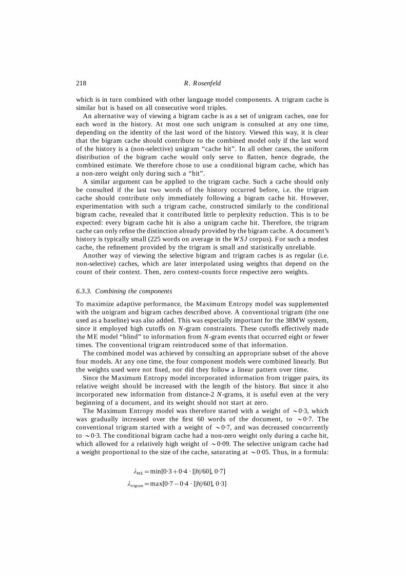
which is in turn combined with other language model components. A trigram cache issimilar but is based on all consecutive word triples.
An alternative way of viewing a bigram cache is as a set of unigram caches, one foreach word in the history. At most one such unigram is consulted at any one time,depending on the identity of the last word of the history. Viewed this way, it is clearthat the bigram cache should contribute to the combined model only if the last wordof the history is a (non-selective) unigram “cache hit”. In all other cases, the uniformdistribution of the bigram cache would only serve to flatten, hence degrade, thecombined estimate. We therefore chose to use a conditional bigram cache, which hasa non-zero weight only during such a “hit”.
A similar argument can be applied to the trigram cache. Such a cache should onlybe consulted if the last two words of the history occurred before, i.e. the trigramcache should contribute only immediately following a bigram cache hit. However,experimentation with such a trigram cache, constructed similarly to the conditionalbigram cache, revealed that it contributed little to perplexity reduction. This is to beexpected: every bigram cache hit is also a unigram cache hit. Therefore, the trigramcache can only refine the distinction already provided by the bigram cache. A document’shistory is typically small (225 words on average in the WSJ corpus). For such a modestcache, the refinement provided by the trigram is small and statistically unreliable.
Another way of viewing the selective bigram and trigram caches is as regular (i.e.non-selective) caches, which are later interpolated using weights that depend on thecount of their context. Then, zero context-counts force respective zero weights.
6.3.3. Combining the components
To maximize adaptive performance, the Maximum Entropy model was supplementedwith the unigram and bigram caches described above. A conventional trigram (the oneused as a baseline) was also added. This was especially important for the 38MW system,since it employed high cutoffs on N-gram constraints. These cutoffs effectively madethe ME model “blind” to information from N-gram events that occurred eight or fewertimes. The conventional trigram reintroduced some of that information.
The combined model was achieved by consulting an appropriate subset of the abovefour models. At any one time, the four component models were combined linearly. Butthe weights used were not fixed, nor did they follow a linear pattern over time.
Since the Maximum Entropy model incorporated information from trigger pairs, itsrelative weight should be increased with the length of the history. But since it alsoincorporated new information from distance-2 N-grams, it is useful even at the verybeginning of a document, and its weight should not start at zero.
The Maximum Entropy model was therefore started with a weight of >0·3, whichwas gradually increased over the first 60 words of the document, to >0·7. Theconventional trigram started with a weight of >0·7, and was decreased concurrentlyto>0·3. The conditional bigram cache had a non-zero weight only during a cache hit,which allowed for a relatively high weight of >0·09. The selective unigram cache hada weight proportional to the size of the cache, saturating at>0·05. Thus, in a formula:
kME=min[0·3+0·4 · [|h|/60], 0·7]
ktrigram=max[0·7−0·4 · [|h|/60], 0·3]

219A ME approach to adaptive statistical language modelling
T XII. Best within domain adaptation perplexity (PP) results. Note that the adaptive modeltrained on 5 million words is almost as good as the baseline model trained on 38 million words
Vocabulary Top 20 000 words of WSJ corpusTest set 325KWTraining set 1MW 5MW 38MW
PP % change PP % change PP % changeTrigram (baseline) 269 — 173 — 105 —Trigram+caches 193 −28% 133 −23% 88 −17%Maximum Entropy (ME): 203 −24% 123 −29% 86 −18%ME+trigram: 191 −29% 118 −32% 75 −28%ME+trigram+caches: 163 −39% 108 −38% 71 −32%
kunigram cache=min[0·001 · |selective unigram cache|, 0·050] (40)
kbigram cache=G0·090
if last word in h also occurred earlier in hotherwise
The threshold for words to enter the selective unigram cache was a static unigramprobability of at least 0·001. The weights were always normalized to sum to 1.
While the general weighting scheme was chosen based on the considerations discussedabove, the specific values of the weights were chosen by minimizing perplexity of unseendata.
6.3.4. Results and analysis
Table XII summarizes perplexity (PP) performance of various combinations of thetrigram model, the Maximum Entropy model (ME), and the unigram and bigramcaches, as follows:
• trigram: this is the static perplexity, which serves as the baseline.• trigram+caches: these experiments represent the best adaptation achievable without
the Maximum Entropy formalism (using a non-selective unigram cache results in aslightly higher perplexity). Note that improvement due to the caches is greater withless data. This can be explained as follows: the amount of information provided bythe caches is independent of the amount of training data, and is therefore fixedacross the three systems. However, the 1MW system has higher perplexity, andtherefore the relative improvement provided by the caches is greater. Put anotherway, models based on more data are better, and therefore harder to improve on.
• Maximum Entropy: these numbers are reproduced from Table X. The relativeadvantage of the “pure” Maximum Entropy model seems greater with more trainingdata (except that the 38MW system is penalized by its high cutoffs). This is becauseME uses constraint functions to capture correlations in the training data. The moredata, the more N-gram and trigger correlations exist that are statistically reliable, andthe more constraints are employed. This is also true with regard to the conventional N-grams in the baseline trigram model. The difference is thus in the number of distance-2 N-grams and trigger pairs.

220 R. Rosenfeld
T XIII. Degradation in quality of language modelling when thetest data is from a different domain than the training data. The trigramhit ratio is relative to a “compact” trigram
Vocabulary Top 20 000 words of WSJ corpusTraining set WSJ (38MW)Test set WSJ (325KW) AP (420KW)
OOV rate 2·2% 3·9%trigram hit rate 60% 50%trigram perplexity 105 206
• ME+trigram: when the Maximum Entropy model is interpolated with the con-ventional trigram, the most significant perplexity reduction occurs in the 38MWsystem. This is because the 38MW ME model employed high N-gram cutoffs, andwas thus “blind” to low count N-gram events. Interpolation with the conventionaltrigram reintroduced some of that information, although not in an optimal form(since linear interpolation is suboptimal) and not for the distance-2 N-grams.
• ME+trigram+caches: these experiments represent the best adaptive scheme weachieved. As before, improvement due to the caches is smaller with more data.Compared with the trigram+caches experiment, the addition of the ME componentimproves perplexity by a relative 16% for the 1MW system, and by a relative 19%for the 5MW and 38MW systems.
To illustrate the success of our within-domain adaptation scheme, note that the bestadaptive model trained on 1 million words is better than the baseline model trainedon 5 million words, and the best adaptive model trained on 5 million words is almostas good as the baseline model trained on 38 million words. This is particularlynoteworthy because the amount of training data available in various domains is oftenlimited. In such cases, adaptation provides handy compensation.
6.4. Cross-domain adaptation
6.4.1. The need for cross-domain adaptationUnder the cross-domain adaptation paradigm, the training and test data are assumedto come from different sources. When this happens, the result is a significant degradationin language modelling quality. The further apart the two language sources are, thebigger the degradation. This effect can be quite strong even when the two sources aresupposedly similar. Consider the example in Table XIII. Training data consists ofarticles from the Wall Street Journal (1987–1989). Test data is made of Associated Press(AP) wire stories from the same period. The two sources can be considered very similar(especially relative to other sources such as technical literature, fine literature, broadcast,etc.). And yet, perplexity of the AP data is twice that of WSJ data.
A related phenomenon in cross-domain modelling is the increased rate of Out-Of-Vocabulary words. In the WSJ-AP example, cross-domain OOV rate is almost doublethe within-domain rate. Similarly, the rate of new bigrams and trigrams also increases(here reported by the complement measure, trigram hit rate, relative to a “compact”trigram, where training-set singletons were excluded).
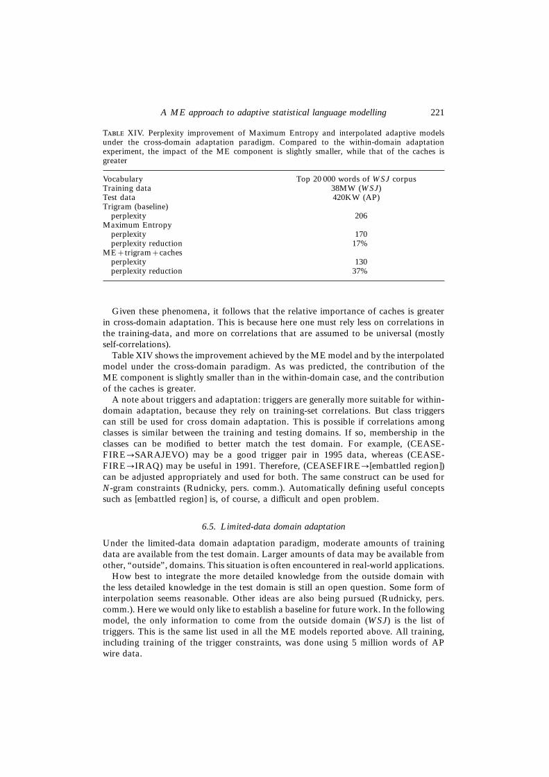
221A ME approach to adaptive statistical language modelling
T XIV. Perplexity improvement of Maximum Entropy and interpolated adaptive modelsunder the cross-domain adaptation paradigm. Compared to the within-domain adaptationexperiment, the impact of the ME component is slightly smaller, while that of the caches isgreater
Vocabulary Top 20 000 words of WSJ corpusTraining data 38MW (WSJ)Test data 420KW (AP)Trigram (baseline)
perplexity 206Maximum Entropy
perplexity 170perplexity reduction 17%
ME+trigram+cachesperplexity 130perplexity reduction 37%
Given these phenomena, it follows that the relative importance of caches is greaterin cross-domain adaptation. This is because here one must rely less on correlations inthe training-data, and more on correlations that are assumed to be universal (mostlyself-correlations).
Table XIV shows the improvement achieved by the ME model and by the interpolatedmodel under the cross-domain paradigm. As was predicted, the contribution of theME component is slightly smaller than in the within-domain case, and the contributionof the caches is greater.
A note about triggers and adaptation: triggers are generally more suitable for within-domain adaptation, because they rely on training-set correlations. But class triggerscan still be used for cross domain adaptation. This is possible if correlations amongclasses is similar between the training and testing domains. If so, membership in theclasses can be modified to better match the test domain. For example, (CEASE-FIRE→SARAJEVO) may be a good trigger pair in 1995 data, whereas (CEASE-FIRE→IRAQ) may be useful in 1991. Therefore, (CEASEFIRE→[embattled region])can be adjusted appropriately and used for both. The same construct can be used forN-gram constraints (Rudnicky, pers. comm.). Automatically defining useful conceptssuch as [embattled region] is, of course, a difficult and open problem.
6.5. Limited-data domain adaptation
Under the limited-data domain adaptation paradigm, moderate amounts of trainingdata are available from the test domain. Larger amounts of data may be available fromother, “outside”, domains. This situation is often encountered in real-world applications.
How best to integrate the more detailed knowledge from the outside domain withthe less detailed knowledge in the test domain is still an open question. Some form ofinterpolation seems reasonable. Other ideas are also being pursued (Rudnicky, pers.comm.). Here we would only like to establish a baseline for future work. In the followingmodel, the only information to come from the outside domain (WSJ) is the list oftriggers. This is the same list used in all the ME models reported above. All training,including training of the trigger constraints, was done using 5 million words of APwire data.

222 R. Rosenfeld
T XV. Perplexity improvement of Maximum Entropy and interpolated adaptive modelsunder the limited-data domain adaptation paradigm. Compared with the within-domain case,the impact of the ME component is somewhat diminished
Vocabulary Top 20 000 words of WSJ corpusTrigger derivation data 38MW (WSJ)Training data 5MW (AP)Test data 420KW (AP)Trigram (baseline)
perplexity 170Maximum Entropy
perplexity 135perplexity reduction 21%
ME+trigram+cachesperplexity 114perplexity reduction 33%
Table XV shows the results. Compared with the within-domain case, the impact ofthe ME component is somewhat diminished, although it is still strong.
7. Adaptive modelling and speech recognition accuracy
Perhaps the most prominent use of language modelling is in automatic speech re-cognition. In this section, we report on the effect of our improved models on theperformance of SPHINX-II, Carnegie Mellon’s speech recognition system. A moredetailed exposition, including a discussion of LM interface issues, can be found inRosenfeld (1994b: chapter 7).
7.1. Within-domain adaptation
To evaluate recognition error rate reduction under the within-domain adaptationparadigm, we used the ARPA CSR (Continuous Speech Recognition) S1 evaluationset of November 1993 (Hwang et al., 1994; Kubala et al., 1994; Pallet et al., 1994). Itconsisted of 424 utterances produced in the context of complete long documents bytwo male and two female speakers. The version of SPHINX-II (Huang et al., 1993b)used for this experiment had gender-dependent 10K senone acoustic models (see Huanget al., 1993a). In addition to the>20 000 words in the standard WSJ lexicon, 178 out-of-vocabulary words and their correct phonetic transcriptions were added in order tocreate closed vocabulary conditions. The forward and backward passes of SPHINX-IIwere first run to create word lattices, which were then used by three independent best-first passes. The first such pass used the 38MW static trigram language model, andserved as the baseline. The other two passes used the interpolated adaptive languagemodel, which was based on the same 38 million words of training data. The first ofthese two adaptive runs was for unsupervised word-by-word adaptation, in which therecognizer’s output was used to update the language model. The other run usedsupervised adaptation, in which the recognizer’s output was used for within-sentence
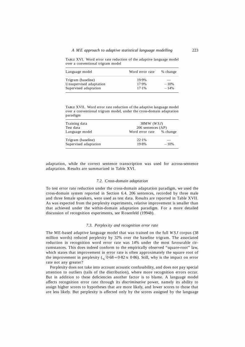
223A ME approach to adaptive statistical language modelling
T XVI. Word error rate reduction of the adaptive language modelover a conventional trigram model
Language model Word error rate % change
Trigram (baseline) 19·9% —Unsupervised adaptation 17·9% −10%Supervised adaptation 17·1% −14%
T XVII. Word error rate reduction of the adaptive language modelover a conventional trigram model, under the cross-domain adaptationparadigm
Training data 38MW (WSJ)Test data 206 sentences (AP)Language model Word error rate % change
Trigram (baseline) 22·1% —Supervised adaptation 19·8% −10%
adaptation, while the correct sentence transcription was used for across-sentenceadaptation. Results are summarized in Table XVI.
7.2. Cross-domain adaptation
To test error rate reduction under the cross-domain adaptation paradigm, we used thecross-domain system reported in Section 6.4. 206 sentences, recorded by three maleand three female speakers, were used as test data. Results are reported in Table XVII.As was expected from the perplexity experiments, relative improvement is smaller thanthat achieved under the within-domain adaptation paradigm. For a more detaileddiscussion of recognition experiments, see Rosenfeld (1994b).
7.3. Perplexity and recognition error rate
The ME-based adaptive language model that was trained on the full WSJ corpus (38million words) reduced perplexity by 32% over the baseline trigram. The associatedreduction in recognition word error rate was 14% under the most favourable cir-cumstances. This does indeed conform to the empirically observed “square-root” law,which states that improvement in error rate is often approximately the square root ofthe improvement in perplexity (J0·68=0·82≈ 0·86). Still, why is the impact on errorrate not any greater?
Perplexity does not take into account acoustic confusability, and does not pay specialattention to outliers (tails of the distribution), where more recognition errors occur.But in addition to these deficiencies another factor is to blame. A language modelaffects recognition error rate through its discriminative power, namely its ability toassign higher scores to hypotheses that are more likely, and lower scores to those thatare less likely. But perplexity is affected only by the scores assigned by the language
224 R. Rosenfeld
model to likely hypotheses—those that are part of a test set, which typically consistsof “true” sentences. Thus a language model that overestimates probabilities of unlikelyhypotheses is not directly penalized by perplexity. The only penalty is indirect, sinceassigning high probabilities to some hypotheses means a commensurate reduction inthe total probability assigned to all other hypotheses. If overestimation is confined toa small portion of the probability space, the effect on perplexity would be negligible.Yet such a model can give rise to significant recognition errors, because the high scoresit assigns to some unlikely hypotheses may cause the latter to be selected by therecognizer.
I am grateful to Peter Brown, Stephen Della Pietra, Vincent Della Pietra, Bob Mercer and SalimRoukos for introducing me to the Maximum Entropy principle and encouraging me to makeuse of their latest developments; to Raymond Lau and Salim Roukos for collaboration on thefirst implementation of the ME training procedure; to David Evans and Steve Henderson forproviding me with the “morphe” program; to the speech group and others at Carnegie Mellonfor varied logistical help, and to Raj Reddy and Xuedong Huang for much appreciated supportand encouragement. Finally, I am grateful to three anonymous reviewers for very useful commentsand suggestions.
This research was supported by the Department of the Navy, Naval Research Laboratoryunder grant no. N00014-93-1-2005. The views and conclusions contained in this document arethose of the author and should not be interpreted as representing the official policies, eitherexpressed or implied, of the U.S. Government.
References
Abramson, N. (1963). Information Theory and Coding. New York: McGraw-Hill.Bahl, L., Jelinek, F. & Mercer, R. (1983). A maximum likelihood approach to continuous speech
recognition. IEEE Transactions on Pattern Analysis and Machine Intelligence PAMI-5, 179–190.Brown, P., DellaPietra, S., DellaPietra, V., Mercer, R., Nadas, A. & Roukos, S. (1994). A maximum
penalized entropy construction of conditional log-linear language and translation models using learnedfeatures and a generalized csiszar algorithm. Unpublished IBM research report.
Brown, P. F., DellaPietra, V. J., deSouza, P. V., Lai, J. C. & Mercer, R. L. (1990). Class-based N-grammodels of natural language. Proceedings of the IBM Natural Language ITL, March, Paris, France.
Chase, L., Rosenfeld, R. & Ward, W. (1994). Error-responsive modifications to speech recognizers:negative N-grams. Proceedings of the International Conference on Spoken Language Processing,September, Yokohama, Japan.
Church, K. & Hanks, P. (1990). Word association norms, mutual information, and lexicography.Computational Linguistics 16, 22–29.
Cover, T. M. & King, R. C. (1978). A convergent gambling estimate of the entropy of English. IEEETransactions on Information Theory IT-24, 413–421.
Darroch, J. N. & Ratcliff, D. (1972). Generalized iterative scaling for log-linear models. The Annals ofMathematical Statistics 43, 1470–1480.
DellaPietra, S., DellaPietra, V., Mercer, R. & Roukos, S. (1992). Adaptive language modelling usingminimum discriminant estimation. Proceedings of the International Conference on Acoustics, Speech andSignal Processing, pp. I-633–636, March, San Francisco, CA. Also published in Proceedings of theDARPA Workshop on Speech and Natural Language. San Mateo, CA: Morgan Kaufmann, pp.103–106.
Dempster, A. P., Laird, N. M. & Rubin, D. B. (1977). Maximum likelihood from incomplete data via theEM algorithm. Journal of the Royal Statistical Society 39, 1–38.
Derouault, A.-M. & Merialdo, B. (1986). Natural language modeling for phoneme-to-text transcription.IEEE Transactions on Pattern Analysis and Machine Translation PAMI-8, 742–749.
Good, I. J. (1953). The population frequencies of species and the estimation of population parameters.Biometrika 40, 237–264.
Good, I. J. (1963). Maximum entropy for hypothesis formulation, especially for multidimensionalcontingency tables. Annals of Mathematical Statistics 34, 911–934.
Huang, X., Alleva, F., Hwang, M.-Y. & Rosenfeld, R. (1993a). An overview of the SPHINX-II speechrecognition system. Proceedings of the ARPA Human Language Technology Workshop, published asHuman Language Technology, pp. 81–86. San Francisco, CA: Morgan Kaufmann.

225A ME approach to adaptive statistical language modelling
Huang, X., Alleva, F., Hon, H.-W., Hwang, M.-Y., Lee, K.-F. & Rosenfeld, R. (1993b). The SPHINX-IIspeech recognition system: an overview. Computer, Speech and Language 2, 137–148.
Hwang, M.-Y., Rosenfeld, R., Thayer, E., Mosur, R., Chase, L., Weide, R., Huang, X. & Alleva, F.(1994). Improved Acoustic and Adaptive Language Models for Continuous Speech Recognition. InProceedings of the ARPA Spoken Language Technologies Workshop, March.
Jaynes, E. T. (1957). Information theory and statistical mechanics. Physics Reviews 106, 620–630.Jelinek, F. (1989). Self-organized language modelling for speech recognition. In Readings in Speech
Recognition (Waibel, A. & Lee, K.-F., eds). San Francisco, CA: Morgan Kaufmann.Jelinek, F. (1991). Up from trigrams! Eurospeech.Jelinek, F., Mercer, R. L., Bahl, L. R. & Baker, J. K. (1977). Perplexity—a measure of difficulty of speech
recognition tasks. 94th Meeting of the Acoustic Society of America, December, Miami Beach, FL.Jelinek, F. & Mercer, R. (1980). Interpolated estimation of Markov source parameters from sparse data.
In Pattern Recognition in Practice (Gelsema, E. S. & Kanal, L. N., eds), pp. 381–402. Amsterdam:North Holland.
Jelinek, F., Merialdo, B., Roukos, S. & Strauss, M. (1991). A dynamic language model for speechrecognition. In Proceedings of the DARPA Workshop on Speech and Natural Language, pp. 293–295,February.
Katz, S. M. (1987). Estimation of probabilities from sparse data for the language model component of aspeech recognizer. IEEE Transactions on Acoustics, Speech and Signal Processing ASSP-35, 400–401.
Kneser, R. & Ney, H. (1991). Forming word classes by statistical clustering for statistical languagemodelling. Proceedings of the 1st QUALICO Conference, September, Trier, Germany.
Kneser, R. & Ney, H. (1995). Improved smoothing for M-gram language modeling. Proceedings of theInternational Conference on Acoustics, Speech and Signal Processing, May, Detroit, MI.
Kubala, F. & members of the CSR Corpus Coordinating Committee (CCCC) (1994). The hub and spokeparadigm for CSR evaluation. Proceedings of the ARPA Workshop on Human Language Technology, pp.40–44. San Francisco, CA: Morgan Kaufmann.
Kuhn, R. (1988). Speech recognition and the frequency of recently used words: a modified Markov modelfor natural language. 12th International Conference on Computational Linguistics [COLING 88], pp.348–350, August, Budapest.
Kuhn, R. & De Mori, R. (1990). A cache-based natural language model for speech recognition. IEEETransactions on Pattern Analysis and Machine Intelligence PAMI-12, 570–583.
Kuhn, R. & De Mori, R. (1992). Correction to a cache-based natural language model for speechrecognition. IEEE Transactions on Pattern Analysis and Machine Intelligence PAMI-14, 691–692.
Kullback, S. (1959). Information Theory in Statistics. New York, NY: Wiley.Kupiec, J. (1989). Probabilistic models of short and long distance word dependencies in running text.
Proceedings of the DARPA Workshop on Speech and Natural Language, pp. 290–295, February.Lau, R. (1993). Maximum likelihood maximum entropy trigger language model. Bachelor’s Thesis,
Massachusetts Institute of Technology, MA.Lau, R., Rosenfeld, R. & Roukos, S. (1993a). Trigger-based language models: a maximum entropy
approach. Proceedings of the International Conference on Acoustics, Speech and Signal Processing,pp. II45–48, April, Minneapolis, MN.Lau, R., Rosenfeld, R. & Roukos, S. (1993b). Adaptive language modeling using the maximum entropy
principle. Proceedings of the ARPA Human Language Technology Workshop, published as HumanLanguage Technology, pp. 108–113. San Francisco, CA: Morgan Kaufmann.
Pallett, D. S., Fiscus, J. G., Fisher, W. M., Garofolo, J. S., Lund, B. & Pryzbocki, M. (1993). Benchmarktests for the ARPA spoken language program. Proceedings of the ARPA Workshop on Human LanguageTechnology, pp. 51–73. March, San Francisco, CA: Morgan Kaufmann.
Paul, D. B. & Baker, J. M. (1992). The design for the Wall Street Journal-based CSR corpus. InProceedings of the DARPA SLS Workshop, February.
Price, P. (1990). Evaluation of spoken language systems: the ATIS domain. Proceedings of the ThirdDARPA Speech and Natural Language Workshop (Stern, R., ed.). San Francisco, CA: MorganKaufmann.
Ratnaparkhi, A. & Roukos, S. (1994). A maximum entropy model for prepositional phrase attachment.Proceedings of the ARPA Workshop on Human Language Technology, pp. 242–242e, March. SanFrancisco, CA: Morgan Kaufmann.
Rosenfeld, R. (1992). Adaptive statistical language modeling: a maximum entropy approach. Ph.D. ThesisProposal, Carnegie Mellon University, Pittsburgh, PA.
Rosenfeld, R. (1994a). A hybrid approach to adaptive statistical language modeling. Proceedings of theARPA Workshop on Human Language Technology, pp. 76–81, March. San Francisco, CA: MorganKaufmann.
Rosenfeld, R. (1994). Adaptive statistical language modeling: a maximum entropy approach. Ph.D. thesis,Carnegie Mellon University, Pittsburgh, PA. Also published as Technical Report CMU-CS-94-138,School of Computer Sciences, Carnegie Mellon University, Pittsburgh, PA.
Rosenfeld, R. & Huang, X. (1992). Improvements in stochastic language modelling. Proceedings of the

226 R. Rosenfeld
DARPA Workshop on Speech and Natural Language, pp. 107–111, February. San Francisco, CA:Morgan Kaufmann.
Shannon, C. E. (1948). A mathematical theory of communication. Bell Systems Technical Journal 27,379–423 (Part I), 623–656 (Part II).
Shannon, C. E. (1951). Prediction and entropy of printed English. Bell Systems Technical Journal 30,50–64.
Suhm, B. & Waibel, A. (1994). Towards better language models for spontaneous speech. ICSLP 94 2,831–834.
Ward, W. (1990). The CMU air travel information service: understanding spontaneous speech. Proceedingsof the DARPA Speech and Natural Language Workshop, pp. 127–129, June.
Ward, W. (1991). Evaluation of the CMU ATIS system. Proceedings of the DARPA Speech and NaturalLanguage Workshop, pp. 101–105, February.
(Received 6 February 1996 and accepted for publication 22 May 1996)
Appendix: The ARPA WSJ language corpus
The first ARPA CSR Wall Street Journal corpus consists of articles published in theWall Street Journal from December 1986 through November 1989. The original datawas obtained, conditioned and processed for linguistic research by the Association forComputational Linguistics’ Data Collection Initiative (ACL/DCI). The corpus waschosen by the ARPA speech recognition community to be the basis for its CSR(Continuous Speech Recognition) common evaluation project. Subsequently, most ofthe data was further processed by Doug Paul at MIT’s Lincoln Labs (Paul & Baker,1992), and conditioned for use in speech recognition. This included transforming manycommon text constructs to the way they are likely to be said when read aloud (e.g.“$123·45” might be transformed into “A hundred and twenty three dollars and fortyfive cents”), some quality filtering, preparation of various standard vocabularies, andmuch more. We refer to this data set as the “WSJ” corpus.
The version of this corpus used in the experiments described in this paper is the onewhere punctuation marks were assumed not to be verbalized, and were thus removedfrom the data. This was known as the “nvp” (non-verbalized-punctuation) condition.In this form, the WSJ corpus contained some 41·5 million words.
All our experiments (except where stated otherwise) used the “20o” vocabulary,which was derived as the most frequent 19 979 non-vp words in the data. It includesall words that occurred at least 60 times in that corpus (and five that occurred 59times). All other words were mapped to a unique symbol, “οUNKπ”, which was madepart of the vocabulary, and had a frequency of about 2·2%. The pseudo word “ο/sπ”was added to the vocabulary to designate end-of-sentence. The pseudo word “οsπ” wasused to designate beginning-of-sentence, but was not made part of the vocabulary.Following are the top and bottom of the vocabulary, in order of descending frequency,together with the words’ count in the corpus:
THE 2322098ο/sπ 1842029OF 1096268TO 1060667A 962706AND 870573IN 801787THAT 415956FOR 408726ONE 335366IS 318271

227A ME approach to adaptive statistical language modelling
SAID 301506DOLLARS 271557IT 256913. . .. . .. . .ARROW’S 60ARDUOUS 60APPETITES 60ANNAPOLIS 60ANGST 60ANARCHY 60AMASS 60ALTERATIONS 60AGGRAVATE 60AGENDAS 60ADAGE 60ACQUAINTED 60ACCREDITED 60ACCELERATOR 60ABUSERS 60WRACKED 59WOLTERS 59WIMP 59WESTINGHOUSE’S 59WAIST 59
A fraction of the WSJ corpus (about 10%), in paragraph units, was set aside foracoustic training and for system development and evaluation. The rest of the data wasdesignated for language model development by the ARPA sites. It consisted of some38·5 million words.
From this set, we set aside about 0·5 million words for language model testing, takenfrom two separate time periods well within the global time period (July 1987 andJanuary–February 1988). The remaining data are the 38 million words used in the largemodels. Smaller models were trained on appropriate subsets.
Our language training set had the following statistics:
• >87 000 article.• >750 000 paragraphs.• >1·8 million sentences (only two sentences/paragraph, on average).• >38 million words (some 450 words/article, on average).
Most of the data were well-behaved, but there were some extremes:
• maximum number of paragraphs per article: 193;• maximum number of sentences per paragraph: 51;• maximum number of words per sentence: 257;• maximum number of words per paragraph: 1483;• maximum number of words per article: 6738.
Following are all the bigrams which occurred more than 65 535 times in the corpus:
318432 οUNKπ ο/sπ669736 οUNKπ οUNKπ83416 οUNKπ A192159 οUNKπ AND

228 R. Rosenfeld
111521 οUNKπ IN174512 οUNKπ OF139056 οUNKπ THE119338 οUNKπ TO170200 οsπ οUNKπ66212 οsπ BUT75614 οsπ IN281852 οsπ THE161514 A οUNKπ148801 AND οUNKπ76187 FOR THE72880 IN οUNKπ173797 IN THE110289 MILLION DOLLARS144923 MR. οUNKπ83799 NINETEEN EIGHTY153740 OF οUNKπ217427 OF THE65565 ON THE366931 THE οUNKπ127259 TO οUNKπ72312 TO THE89184 U. S.
The most frequent trigram in the training data occurred 14 283 times. It was:
οsπ IN THE