a measurement metric for forensic latent fingerprint ... this new sivv-based metric for latent...
TRANSCRIPT

This publication is available free of charge from http://dx.doi.org/10.6028/NIST.IR.8017
NISTIR 8017
A Measurement Metric for Forensic
Latent Fingerprint Preprocessing
Haiying Guan
Andrew Dienstfrey
Mary Theofanos
Brian Stanton
http://dx.doi.org/10.6028/NIST.IR.8017

This publication is available free of charge from http://dx.doi.org/10.6028/NIST.IR.8017
NISTIR 8017
A Measurement Metric for Forensic
Latent Fingerprint Preprocessing
Haiying Guan
Brian Stanton
Information Access Division
Information Technology Laboratory
Andrew Dienstfrey
Applied and Computational Mathematics Division
Information Technology Laboratory
Mary Theofanos
Office of Data and Informatics
Material Measurement Laboratory
This publication is available free of charge from:
http://dx.doi.org/10.6028/NIST.IR.8017
July 2014
U.S. Department of Commerce
Penny Pritzker, Secretary
National Institute of Standards and Technology
Willie E. May, Acting Under Secretary of Commerce for Standards and Technology and Acting Director

This publication is available free of charge from http://dx.doi.org/10.6028/NIST.IR.8017
NISTIR 8017 Page ii 7/2014
TABLE OF CONTENTS
1 INTRODUCTION ...................................................................................................................................... 1
1.1 FORENSIC LATENT FINGERPRINT .............................................................................................................. 1 1.2 LATENT FINGERPRINT PREPROCESSING ..................................................................................................... 1 1.3 THE SOFTWARE AND TOOLS FOR LATENT FINGERPRINT PREPROCESSING ................................................... 4
2 METHOD .................................................................................................................................................... 5
2.1 LITERATURE REVIEW ................................................................................................................................ 5 2.2 METHOD OVERVIEW ................................................................................................................................. 5 2.3 SIVV ON FLAT/TEN-PRINT OR ROLLED FINGERPRINT ................................................................................ 6 2.4 MOTIVATION OF OUR APPROACH ............................................................................................................ 10 2.5 BLACKMAN WINDOW.............................................................................................................................. 12 2.6 REGION OF INTEREST (ROI) ..................................................................................................................... 15 2.7 PEAK LOCATION CONSTRAINT ................................................................................................................ 17 2.8 SOME PROPERTIES OF THE SIVV ............................................................................................................ 19
2.8.1 Image inversion ............................................................................................................................ 19 2.8.2 SIVV on noise images .................................................................................................................. 22
3 EXPERIMENTAL RESULTS ................................................................................................................ 24
3.1 LATENT FINGERPRINT PREPROCESSING DATASET ................................................................................... 24 3.2 LATENT FINGERPRINT QUALITY MEASUREMENT ..................................................................................... 26
3.2.1 Region of interest ......................................................................................................................... 26 3.2.2 Peak location constraint ............................................................................................................... 27
3.3 COMPARISON RESULTS ........................................................................................................................... 30
4 DISCUSSION AND FUTURE WORK................................................................................................... 31
5 ACKNOWLEDGEMENTS ..................................................................................................................... 33
6 DISCLAIMER .......................................................................................................................................... 33
7 REFERENCES ......................................................................................................................................... 33
APPENDIX A: THE SIVV PEAK ON SYNTHETIC IMAGES ................................................................... 37

This publication is available free of charge from http://dx.doi.org/10.6028/NIST.IR.8017
NISTIR 8017 Page iii 7/2014
LIST OF TABLES AND FIGURES
TABLE 1: THE COMPARISON OF DIFFERENT ALGORITHMS WITH DIFFERENT OPTIONS ............................................ 31
TABLE 2: SIVV PEAK LOCATIONS ON THE IMAGES WITH THE STRIPES PATTERN (IMAGE SIZE 512×512 PIXELS) ... 40
TABLE 3: SIVV PEAK LOCATIONS ON THE LARGE IMAGES WITH THE STRIPES PATTERN (IMAGE SIZE 1024×1024
PIXELS) ........................................................................................................................................................ 41
TABLE 4: THE RELATIONSHIP BETWEEN PEAK LOCATIONS AND PPI ...................................................................... 41
TABLE 5: THE PEAK LOCATIONS GIVEN THE STRIPE PIXEL DISTANCE. ................................................................... 41
FIGURE 1: AN EXAMPLE OF FORENSIC LATENT FINGERPRINT PREPROCESSING. ....................................................... 2
FIGURE 2: THE NECESSITY OF LATENT FINGERPRINT PREPROCESSING. ................................................................... 3
FIGURE 3: DISTINCT ENDPOINTS OF FORENSIC LATENT FINGERPRINT PREPROCESSING. ........................................... 4
FIGURE 4: SIVV ALGORITHM. ................................................................................................................................. 8
FIGURE 5: AN EXAMPLE OF SIVV FEATURE ON A ROLLED FINGERPRINT IMAGE. .................................................... 9
FIGURE 6: AN EXAMPLE OF THE SIVV FEATURE ON A LATENT FINGERPRINT IMAGE. ............................................ 10
FIGURE 7: EXAMPLES OF THE SIVV FEATURE ON LATENT FINGERPRINT IMAGES. ................................................. 12
FIGURE 8: BLACKMAN WINDOW (Α = 0.16). ......................................................................................................... 13
FIGURE 9: THE COMPARISON OF SIVV CURVES WITH DIFFERENT INPUT OPTIONS. ................................................ 14
FIGURE 10: THE SELECTION OF REGION OF INTEREST. .......................................................................................... 15
FIGURE 11: AN EXAMPLE OF REGION OF INTEREST. .............................................................................................. 16
FIGURE 12: AN EXAMPLE OF SIVV PEAK LOCATION CONSTRAINT. ....................................................................... 18
FIGURE 13: THE ORIGINAL IMAGE AND ITS INVERT IMAGE OF WHITE POWER DEVELOPED PRINTS. ........................ 20
FIGURE 14: THE COMPARISON OF SIVV CURVES OF AN IMAGE AND ITS INVERT IMAGE. ....................................... 21
FIGURE 15: THE IMAGE WITH DIFFERENT LEVELS OF IID RANDOM NOISE. ............................................................ 22
FIGURE 16: THE IMAGE MATRICES WITH RANDOM NOISE. ..................................................................................... 23
FIGURE 17: THE COMPARISON OF SIVV CURVES OF AN IMAGE WITH DIFFERENT LEVELS OF IID RANDOM NOISE. 24
FIGURE 18: THE LATENT FINGERPRINT PREPROCESSING IMAGE PAIRS FROM A TRAINING COURSE (SIX TYPES). ... 25

This publication is available free of charge from http://dx.doi.org/10.6028/NIST.IR.8017
NISTIR 8017 Page iv 7/2014
FIGURE 19: THE PROPOSED ALGORITHM FOR LATENT FINGERPRINT QUALITY MEASUREMENT. ............................ 26
FIGURE 20: THE COMPARISON OF WHOLE IMAGE VS. ROI IMAGE. ........................................................................ 27
FIGURE 21: PEAK LOCATION CONSTRAINT. ........................................................................................................... 28
FIGURE 22: PROPOSED PROCEDURE FOR LATENT FINGERPRINT SIVV FEATURE DETECTION. ................................ 29
FIGURE 23: THE FREQUENCY FEATURE OF LATENT FINGERPRINT USING THE PROPOSED ALGORITHM. .................. 30
FIGURE 24: QUANTITATIVE COMPARISON OF LATENT FINGERPRINT IMAGE QUALITY. .......................................... 32
FIGURE 25: SIVV ON THE IMAGES WITH THE STRIPES PATTERN (IMAGE SIZE 512×512 PIXELS). ........................... 39
FIGURE 26: SIVV ON THE LARGE IMAGES WITH THE STRIPES PATTERN (IMAGE SIZE 1024×1024 PIXELS). ............ 40
FIGURE 27: SIVV ON THE IMAGES WITH SQUARE PATTERN. ................................................................................. 42

This publication is available free of charge from http://dx.doi.org/10.6028/NIST.IR.8017
NISTIR 8017 Page v 7/2014
EXECUTIVE SUMMARY
Although fingerprint mark-up and identification are well-studied fields, forensic fingerprint
image preprocessing is still a relatively new domain in need of further scientific study and
development of best practice guidance. Latent fingerprint image preprocessing is a common
step in the forensic analysis workflow that is performed to improve image quality for
subsequent identification analysis while simultaneously ensuring data integrity. Due to the
low quality of the latent fingerprint images, preprocessing is especially crucial to the success
of the final fingerprint identification in the forensic fingerprint image examination. In this
report, we isolate the forensic fingerprint image preprocessing step for more detailed
analysis.
First we provide a brief review of latent fingerprint image preprocessing. We then turn to the
problem of defining an image-based quality metric suitable for analysis of forensic latent
fingerprint preprocessing. More precisely, we propose to extend Spectral Image Validation
and Verification (SIVV) [1] to serve as a metric for latent fingerprint image quality
measurement. SIVV analysis was originally developed to differentiate ten-print or rolled
fingerprint images from other non-fingerprint images such as face or iris images. Several
modifications are required to extend SIVV analysis to the latent space. We implement and
test this new SIVV-based metric for latent fingerprint image quality and use it to measure the
performance of the forensic latent fingerprint preprocessing step. Preliminary results show
that the new metric can provide positive indications of both latent fingerprint image quality
and the performance of the fingerprint preprocessing.
Keywords:
Forensic latent fingerprint image, Latent fingerprint image quality measurement, Spectral
Image Validation and Verification Metric (SIVV), Latent fingerprint preprocessing,
Fingerprint image enhancement.

This publication is available free of charge from http://dx.doi.org/10.6028/NIST.IR.8017
NISTIR 8017 Page 1 7/2014
1 INTRODUCTION
1.1 FORENSIC LATENT FINGERPRINT
Fingerprints have been used to identify persons for centuries. As one of the most prevalent
and powerful types of forensic evidence that can be recovered during the investigation of a
crime, fingerprints have been routinely used for person identification in crime scenes.
There are different types of fingerprints. Ten-print and rolled fingerprints are captured on a
fingerprint card or by special electronic devices. These fingerprint capture devices generally
have built-in monitoring systems to guarantee the image quality. By contrast to this
controlled capture process, the term latent fingerprints, or latents, refer to fingerprint
impressions that are left unintentionally. Generally latents are partial prints lifted from
surfaces of objects found at crime scenes that are touched or grasped by a person’s fingers.
Lifting of latent fingerprints involves complicated processes. Several chemical and physical
development techniques are available to enhance the visibility of the friction ridge detail
including: photographing the prints under different light sources, dusting with powders, and
chemical processing. Ideally, the enhanced print can be lifted from the substrate and
transferred to a secondary backing material that serves to improve the contrast of the ridges
with respect to the background. While these development techniques improve fingerprint
features, generally latents are of significantly poorer quality compared to rolled prints. This
can depend on the substrate of the original latent impression. For example, when attempting
to lift prints from porous paper substrates such as newsprint, magazines, and wallpaper, the
lifted fingerprints’ quality may be very low in some cases, and they are not usable for
recognition even after preprocessing. Moreover, latent fingerprint backgrounds can exhibit
diverse combinations of color, design, and texture that can mask the identity and spatial
configuration of minutiae in a questioned print. In spite of these drawbacks, latent
fingerprints are extremely useful in forensics to investigate crime scenes [22][23][24][25].
As a widely used biometric, latent fingerprints support an irreplaceable functionality:
fingerprint recognition. Fingerprint recognition is a technique that can link latents to suspects
whose fingerprints were previously enrolled in ten-print or rolled fingerprints databases, or to
link to latent fingerprints from different crime scenes.
1.2 LATENT FINGERPRINT PREPROCESSING
The performance of a fingerprint recognition system is heavily dependent on the quality of
the collected fingerprint images. This poses a problem for latent fingerprints as their image
quality is generally low due to the combination of difficulties in lifting the print from
substrate and image contamination by complex background noise. As a result, fingerprint
structure such as minutiae and ridges may not be clearly visible to the human eye of a
fingerprint examiner, nor easily detected by the algorithms in automatic matching systems.

This publication is available free of charge from http://dx.doi.org/10.6028/NIST.IR.8017
NISTIR 8017 Page 2 7/2014
Due to the poor quality of latent fingerprint images, digital image preprocessing is a
necessary step in the forensic analysis workflow [2]. Image preprocessing is performed to
increase latent fingerprint image quality. Some of the common transformations employed in
service of this goal include: color management, contrast adjustment, edge enhancement,
background suppression, and noise filtration [3] [4] [5] [6] [7] [8] . Figure 1 shows an
example of forensic latent fingerprint image preprocessing: the color image on the left is the
image directly collected from the crime scene, and the gray-level image on the right is the
image after preprocessing.
Clearly the fingerprint in the image after processing (on the right) visually exhibits more
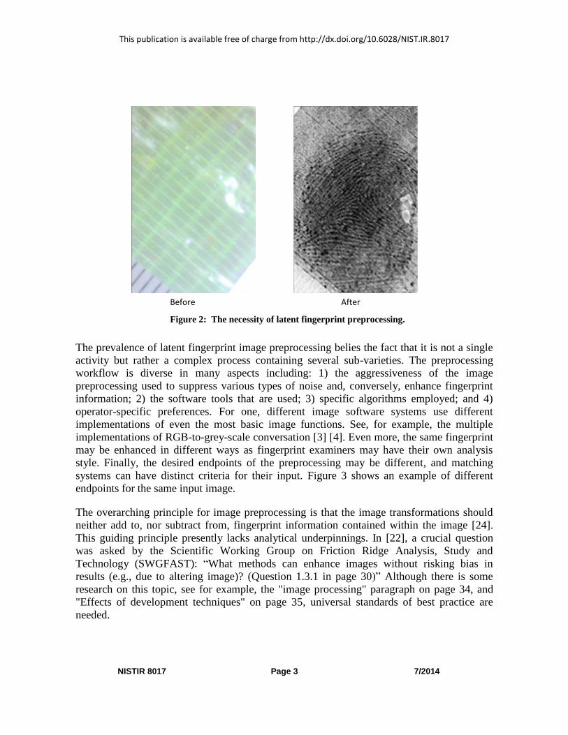
fingerprint pattern information. Figure 2 shows another example in which image
preprocessing is essential. The image on the left shows a crime scene lift in which an
impression is left on duct tape. The grid pattern of the duct tape is clearly visible in a green
hue which, to the eye, completely masks fingerprint information. The image on the right
shows the same latent print image after preprocessing. In this example, preprocessing
included: developing using Basic Yellow (dye stain), color filtering using Channel ‘a’ in the
Photoshop’s Lab Color mode, application of a Fourier-based pattern removal filter (which is
a product of Foray Technologies), and greyscale management with the Photoshop Levels
command. The end result is a preprocessed image that clearly reveals ridge flow.
Before After
Figure 1: An example of forensic latent fingerprint preprocessing.
This publication is available free of charge from http://dx.doi.org/10.6028/NIST.IR.8017
NISTIR 8017 Page 3 7/2014
The prevalence of latent fingerprint image preprocessing belies the fact that it is not a single
activity but rather a complex process containing several sub-varieties. The preprocessing
workflow is diverse in many aspects including: 1) the aggressiveness of the image
preprocessing used to suppress various types of noise and, conversely, enhance fingerprint
information; 2) the software tools that are used; 3) specific algorithms employed; and 4)
operator-specific preferences. For one, different image software systems use different
implementations of even the most basic image functions. See, for example, the multiple
implementations of RGB-to-grey-scale conversation [3] [4]. Even more, the same fingerprint
may be enhanced in different ways as fingerprint examiners may have their own analysis
style. Finally, the desired endpoints of the preprocessing may be different, and matching
systems can have distinct criteria for their input. Figure 3 shows an example of different
endpoints for the same input image.
The overarching principle for image preprocessing is that the image transformations should
neither add to, nor subtract from, fingerprint information contained within the image [24].
This guiding principle presently lacks analytical underpinnings. In [22], a crucial question
was asked by the Scientific Working Group on Friction Ridge Analysis, Study and
Technology (SWGFAST): “What methods can enhance images without risking bias in
results (e.g., due to altering image)? (Question 1.3.1 in page 30)” Although there is some
research on this topic, see for example, the "image processing" paragraph on page 34, and
"Effects of development techniques" on page 35, universal standards of best practice are
needed.
Before After
Figure 2: The necessity of latent fingerprint preprocessing.

This publication is available free of charge from http://dx.doi.org/10.6028/NIST.IR.8017
NISTIR 8017 Page 4 7/2014
The goal of this study is to characterize the effects of image preprocessing that transforms
the latent fingerprint image obtained from the crime scene (‘before image’) to the image used
for identity analysis (‘after image’).
1.3 THE SOFTWARE AND TOOLS FOR LATENT FINGERPRINT
PREPROCESSING
A number of image analysis tools are capable of revealing latent fingerprint information
comingled with noisy background features. The range of applicable software includes:
commercial photo editing tools designed for general purpose image editing such as Adobe
Photoshop and Pixelmator; open source image editing tools such as the GNU Image
Manipulation Program and Inkscape; scientific toolboxes such as the Matlab image
processing toolbox and Open Source Computer Vision; and specialty software particularly
designed for latent fingerprint analysis such as the FBI's Latent Fingerprint Services,
Universal Latent Workstation, Automated Fingerprint Identification System (AFIS)’s
interactive graphical user interface for latent prints, etc. Although there are general common
functions in those software toolboxes, different software tools are designed for different
purposes and used for different applications. Specifically for forensic fingerprint recognition,
we need to define analysis and procedures to verify that the software follows the basic
principle and requirements of latent fingerprint preprocessing, thereby ensuring the
repeatability of the process and guaranteeing image integrity.
(a) Original latent fingerprint
Figure 3: Distinct endpoints of forensic latent fingerprint preprocessing.
(b) After second preprocessing
(c) After first preprocessing

This publication is available free of charge from http://dx.doi.org/10.6028/NIST.IR.8017
NISTIR 8017 Page 5 7/2014
2 METHOD
2.1 LITERATURE REVIEW
Although latent fingerprints are well and widely studied by forensic scientists [3], there has
been little systematic analysis of forensic latent fingerprint image preprocessing. Digital
image preprocessing is a relatively new area requiring research in order to establish its
scientific foundations. It is especially critical to investigate the image transformations used in
the course of this analysis, and to propose effective approaches or give general suggestions to
guide the preprocessing workflow to improve the latent fingerprint quality and preserve the
fingerprint integrity at the same time. The principle objective of this work is to initiate such
investigations.
Latent fingerprint images are obtained under non-ideal acquisition conditions; the finger
impression may be incomplete, distorted, or corrupted by background noise. In most cases,
the latent fingerprint quality is crucial for latent identification. The research community has
developed several approaches and algorithms on fingerprint image quality [11], [12], [14],
[15] and latent fingerprint preprocessing [13]. In [14], a latent fingerprint image quality
(LFIQ) measurement was proposed. In [13], Yoon, et al. proposed a latent fingerprint
enhancement algorithm requiring a manually marked region of interest (ROI) and singular
points. The paper proposed a novel orientation field estimation algorithm, which fits the
coarse orientation map to an orientation field model. Experimental results on the NIST SD27
Latent Fingerprint Database [19] indicate that, with the use of the proposed enhancement
algorithm, the matching accuracy of the commercial matcher, Rank-m identification Rate,
was improved by 5% to 20%.
2.2 METHOD OVERVIEW
We seek to compare the image qualities of before images ˗ original RGB images, directly
obtained from forensic crime scene photography ˗ and after images ˗ the grey scale image
after preprocessing ˗ to evaluate the performance of the preprocessing effect.
In the context of latent fingerprint analysis, a primary objective is to improve contrast
between ridges and furrows, thereby enabling clearer identification of minutia points. The
ridges and furrows appear as periodic structures in the fingerprint image. This periodicity
manifests as narrow regions with relatively high-energy content in the frequency spectrum of
the image. It is natural to construct a latent fingerprint quality metric built on this feature.
Our latent fingerprint quality metric is based on an extension of the Spectral Image
Verification and Validation analysis (SIVV) [1]. The original SIVV algorithm was designed

This publication is available free of charge from http://dx.doi.org/10.6028/NIST.IR.8017
NISTIR 8017 Page 6 7/2014
for image validation and verification of ten-print fingerprint images from live-scan devices,
and for maintaining the fidelity of fingerprint image databases. SIVV can effectively
differentiate the non-fingerprint input from the flat or rolled fingerprint input. As the periodic
structure of the fingerprint ridges and furrows is a level one feature, SIVV is potentially
applicable to the latent fingerprint preprocessing domain. However, latent fingerprint images
are often corrupted by complex background noise, and the ridge structures may not be clearly
visible. Furthermore, latent images are generally of poor quality and the fingerprints can be
incomplete. These characteristics will confound the original SIVV feature analysis;
refinement is needed for SIVV to be applicable to latent fingerprint images.
We implement several modifications to SIVV in light of the above-mentioned difficulties. In
order to suppress confounding background noise, in the spatial domain the algorithm focuses
analysis on a region of interest within the fingerprint image. Furthermore in the frequency
domain, the algorithm constrains the SIVV peak to be within a limited range, which can be
inferred by the fingerprint ridges’ pixel distances on the latent fingerprint images. The
resulting metric is still based on the intrinsic Fourier spectral properties of latent fingerprint
images. The new latent fingerprint quality metric provides the quantitative measurement to
characterize the quality of the latent fingerprint images and measures the effectiveness of the
latent fingerprint preprocessing process.
2.3 SIVV ON FLAT/TEN-PRINT OR ROLLED FINGERPRINT
SIVV analysis derives from the periodicity of ridges and furrows [1]. For completeness, first
we summarize the original SIVV algorithm (for the detailed presentation, please refer to the
original report [1]).
Step 1. Image Windowing
The standard one-dimensional Blackman window is given in the following equation:
𝑤(𝑛) = 0.42 − 0.5 cos (2𝜋𝑛
𝑁 − 1) + 0.08 cos (
4𝜋𝑛
𝑁 − 1) (1)
𝑤ℎ𝑒𝑟𝑒 0 ≤ 𝑛 ≤ 𝑁 − 1
The length of the one-dimensional window is N. The constant numbers in the equation are
the same as the standard Blackman filter. Given the image with N rows and M columns, the
two-dimensional Blackman Window is the tensor product of windows of length N and M.
When the 2D Blackman Window is applied to the fingerprint image, the window is applied
on the center of the fingerprint texture, and the size is adapted to the size of the fingerprint
image.

This publication is available free of charge from http://dx.doi.org/10.6028/NIST.IR.8017
NISTIR 8017 Page 7 7/2014
Step 2. Discrete Fourier Transform (DFT)
𝐻(𝑢, 𝑣) = ∑
𝑀−1
𝑥=0
∑exp [2𝜋𝑖𝑦𝑣
𝑁] exp [2𝜋𝑖𝑥
𝑢
𝑀] ℎ(𝑥, 𝑦)
𝑁−1
𝑦=0
(2)
Here 𝑢 and 𝑣 denote frequency components in the 𝑥 and 𝑦 directions ranging from −𝑀
2 to
𝑀
2
and −𝑁
2 to
𝑁
2 respectively.
Step 3. 2D (normalized) Log Power Spectrum
The 2D power spectrum is computed as:
𝑃(𝑢, 𝑣) = |𝐻(𝑢, 𝑣)|2 (3)
Depending on the implementation, the output of this step can be normalized or not-
normalized; that is
10 ∗ 𝑙𝑜𝑔𝑃(𝑢, 𝑣) (4)
Or
10 ∗ 𝑙𝑜𝑔𝑃(𝑢, 𝑣)
𝑃(0,0) (5)
Step 4. 2D Polar Transform of Power Spectrum
The 2D power spectrum is represented in polar coordinates using the transformation:
𝜌 =√𝑢2 + 𝑣2
√𝑀2 + 𝑁2 (6)
𝜃 = 𝑡𝑎𝑛−1 (𝑣
𝑢) (7)
where the [0, 0] point is in the image center. We use 𝑃(𝜌, 𝜃) to represent the 2D results of
the polar transformation, where 𝜌 is divided by the maximum dimension of the input image
N, normalized to 0 and 0.5 cycles/pixel.
Step 5. 1D Normalized Polar Transform
Finally, the 1D polar transform is computed as the sum over angles of:

This publication is available free of charge from http://dx.doi.org/10.6028/NIST.IR.8017
NISTIR 8017 Page 8 7/2014
𝑃(𝜌) = ∑𝑃(𝜌, 𝜃)
180
𝜃=0
𝜌 = 0,… ,0.5 𝑐𝑦𝑐𝑙𝑒𝑠/𝑝𝑖𝑥𝑒𝑙
(8)
The normalized 1D polar curve is:
𝑃𝑁(𝜌) =𝑃(𝜌)
𝑃(0)
𝜌 = 0,… ,0.5 𝑐𝑦𝑐𝑙𝑒𝑠/𝑝𝑖𝑥𝑒𝑙
(9)
DFT Polar
Transform
10*log(P) or
10*log(P/P0)
2D power
spectrum
2D polar
spectrum
Blackman
Window
Input
image
𝑷𝜽 (𝝆, 𝜽)
/ 𝑷𝜽 (𝟎, 𝜽)
1D polar
spectrum
Filtered
image
Normalized 2D log
power spectrum
Figure 4: SIVV algorithm.

This publication is available free of charge from http://dx.doi.org/10.6028/NIST.IR.8017
NISTIR 8017 Page 9 7/2014
Figure 4 shows the algorithm schematic. Figure 5 shows the analysis step-by-step.1 The
clear peak and valley in the polar power spectrum (sub-figure (g)) is indicative of the ridge-
flow periodicity and is referred to in the following as the SIVV feature.
The original objective of SIVV analysis is to screen fingerprint image databases for
specimens improperly scanned from fingerprint cards [1]. In the auto-capture process, SIVV
analysis can help to identify the auto-capture failures, identify non-fingerprint images that
may have been incorrectly included in a fingerprint database, etc. The original SIVV
algorithm focuses on the fingerprint datasets that were captured under controlled
environments, such as flat/ten-print or rolled fingerprint database, or mixed database which
contains face, iris and fingerprint, etc. Generally, the fingerprints in such datasets have clean
background and significant less noise compared with the latent fingerprint image dataset.
1 Courtesy of SIVV software package in NBIS [1] [20], the original image is G001T2U.tif in [19].
(e) 2D power spectrum (f) 2D polar spectrum (g) 1D polar spectrum
(c) After Blackman window (b) Cropped image (a) Original image
dB
Cycles/pixel
Figure 5: An example of SIVV feature on a rolled fingerprint image.

This publication is available free of charge from http://dx.doi.org/10.6028/NIST.IR.8017
NISTIR 8017 Page 10 7/2014
2.4 MOTIVATION OF OUR APPROACH
The original SIVV feature performs well on the flat/ten-print or rolled fingerprint database,
which are captured by inking methods or live-scan devices in an attended mode. In such
contexts, background noise is minimized during the capture, and the contrast between the
ridges and furrows is relatively high. As image quality is generally controlled very well, the
fingerprint image ridges and valleys are clear and computer-readable. In such cases, the
periodic structure of the ridges and valleys can be captured by Fourier spectrum analysis in
the frequency domain. It follows that SIVV performs well when the original fingerprint
image is of good quality.
In comparison with rolled fingerprints, original latent fingerprint images are of much poorer
quality in several respects. Latent fingerprints are generally smudgy and blurred. They often
capture only a small finger area, and may have large nonlinear distortion due to pressure
variations. Finally, and perhaps the most damaging source of noise from the perspective of
SIVV analysis, in latent fingerprint images, it is not uncommon for the fingerprint image to
be superimposed on a structured background. This background “noise” is unavoidable and is
extremely hard to model due to the large variety of background colors, textures, etc. When
background noise is strong, the spectral spike from the fingerprint periodicity can be
conflated with the signals of other periodic structures of the images. Sources of such
patterned noises are diverse and include textile fabric, written text, and residue from the
(a) Original image (b) Cropped image (c) After Blackman window
(d) 2D power spectrum (e) 2D log polar spectrum (f) 1D log polar spectrum
Figure 6: An example of the SIVV feature on a latent fingerprint image.

This publication is available free of charge from http://dx.doi.org/10.6028/NIST.IR.8017
NISTIR 8017 Page 11 7/2014
physical processing. Figure 6 shows an example2 of original SIVV on a latent fingerprint
image in the NIST Database 27 [19]. It shows that the SIVV spike is largely weakened due to
the fingerprint incompleteness and from being submerged in the background noise.
Figure 7 (implementation courtesy of [20]) shows the results of applying the original SIVV
analysis [20] to six unprocessed, latent fingerprint images taken from a database of training
images provided by Schwarz Forensics and Foray Technologies (the image database is
described in more detail in 3.1). These images demonstrate that the original SIVV analysis
may not be directly applicable to latent fingerprint images. In the cases 1, 3, 5, and 6, there is
no obvious spike (fingerprint level-one information) at all. In cases 2 and 4, the detected
peak (red arrow) does not represent the fingerprint ridges and furrows, but rather arises due
to texture of the background. In addition, 1-c and 2-c show the detailed texture noise (tiny
grids) on the images. The actual fingerprint ridge peak is shown by the green arrows in 2-b
and 4-b.
In this report, we introduce two additional components to the SIVV analysis to regain the
valuable metrical functionality that is otherwise lost in latent fingerprint contexts. First, we
introduce a Region of Interest (ROI) selection to enable the analysis to focus only on a local
subregion which contains fingerprint signal in spatial domain. Second, we introduce a
constraint in the spectral analysis restricting attention to a small window which may contain
the ridge and furrow spike in the frequency domain.
2 Courtesy of SIVV software package in NBIS [1] [20], the original image is G001L2U.tif in [19].

This publication is available free of charge from http://dx.doi.org/10.6028/NIST.IR.8017
NISTIR 8017 Page 12 7/2014
2.5 BLACKMAN WINDOW
In fingerprint analysis, the Blackman window is used to suppress signal outside of the
fingerprint region in addition to eliminating non-periodic boundary effects. The standard 1D
Blackman Window is defined by:
𝑤(𝑛) =1 − 𝛼
2−1
2cos (
2𝜋𝑛
𝑁 − 1) +
𝛼
2cos (
4𝜋𝑛
𝑁 − 1) (10)
1-a. Original image (158) 1-b. 1D log polar spectrum
2-a. Original image (165) 2-b. 1D log polar spectrum
1-c. Zoom in the background noise of (2-a)
2-c. Zoom in the background noise of (3-a)
3-a. Original image 3-b. 1D log polar spectrum 4-a. Original image 4-b. 1D log polar spectrum
5-b. 1D log polar spectrum 5-a. Original image (160) 6-a. Original image 6-b. 1D log polar spectrum
Figure 7: Examples of the SIVV feature on latent fingerprint images.

This publication is available free of charge from http://dx.doi.org/10.6028/NIST.IR.8017
NISTIR 8017 Page 13 7/2014
where 0 ≤ 𝑛 ≤ 𝑁 − 1 and α = 0.16. The resulting curve is shown in (Figure 8). The 2D
Blackman window filter is the cross product of two 1D Blackman window vectors (N maybe
different in two 1D vectors).
In latent images, variability in fingerprint location, orientation, and size requires that we add
more flexibility in application of the Blackman window filter to the image. We include
additional parameters to control the location (center point of the 2D filter), size (if the
fingerprint region is modeled by an ellipse with the ellipse’s major axis of 𝑁𝑚𝑎𝑥 pixels and
minor axis of 𝑁𝑚𝑖𝑛 pixels respectively, the size can be controlled by using 𝑁𝑚𝑎𝑥 and 𝑁𝑚𝑖𝑛
in the Blackman window equation), and orientation (the filter can be rotated in 2D plane) of
the Blackman window. The constant numbers in the Blackman equation control the shape of
the filter. To be faithful to the original Blackman filter, we keep the constant number
unchanged and the curve shape unchanged. In practice, in order to increase the SIVV signal
strength, we like to focus only on the ridge furrow patterns by customizing the size of the
filter window to the size of the fingerprint area, and aligning the Blackman filter center to the
fingerprint center. Figure 9 contrasts the following SIVV results: no Blackman window (a);
original Blackman window (b); and customized Blackman window (by customizing the size,
aligning the location and orientation) (c). We see that the regular Blackman window does
help to strengthen the fingerprint signal in some cases. The customized Blackman Window
has more flexibility to select the best region, which is very useful to latent fingerprint image
analysis as location, orientation, and extent of the print region vary greatly in latent
fingerprint images.
Figure 8: Blackman Window (α = 0.16).

This publication is available free of charge from http://dx.doi.org/10.6028/NIST.IR.8017
NISTIR 8017 Page 14 7/2014
(a) a-1. Original image without Blackman Window (051e)
b-2. Blackman window on whole image (b) b-1.Blackman Window b-3. SIVV on b-2
(c) c-1. Customized Blackman Window c-2. Image after customized Blackman Window c-3. SIVV on c-2
(d) d-1. ROI image [698 62 1519 589]
d-2. Blackman window on ROI image d-3. SIVV on d-2
Figure 9: The comparison of SIVV curves with different input options.
a-2.SIVV on whole image

This publication is available free of charge from http://dx.doi.org/10.6028/NIST.IR.8017
NISTIR 8017 Page 15 7/2014
2.6 REGION OF INTEREST (ROI)
Latent fingerprint images often include significant noise (where noise is defined as any
image feature that is not clearly identifiable as fingerprint information). Noise that overlaps
with fingerprint region is intrinsically harder to diminish while simultaneously maintaining
fingerprint integrity. One exception to this is when the noise is well separated from
fingerprint information in a color space, in which case color filtration can be a powerful and
effective tool. In general, such separation is not the case. For this reason, it is important that
our analysis be designed with a high degree of specificity to fingerprint information. By
contrast, it is relatively easy to remove the background noise in the area outside of the
fingerprint region. Furthermore, it is important to do so as these regions contain no
fingerprint information yet, due to the nonlocal nature of Fourier-based spectral analysis,
they may contribute a large amount of non-signal energy, thereby masking the fingerprint
SIVV feature in the frequency domain. Thus we specify region of interest (ROI) by selecting
a rectangular region containing the entire fingerprint. An example is shown in Figure 10.
Image features outside the ROI are masked by setting the intensity value to a constant black.
This ROI selection is done prior to the FFT step of the SIVV and performed “in place,” i.e.,
the image remains the size of the original, so as to maintain pixel density and not introduce
rescaling artifacts. During the latent fingerprint image quality measurement process, there is
a trade-off between the fingerprint region size and fingerprint region purity. The ROI should
contain most of the area3 of the fingerprint image with good ridge information. Currently the
3 Notice that the ROI proposed here is only for latent fingerprint detection and quality measurement, not for
latent fingerprint identification. The whole fingerprint region should be considered in the identification
process.
Figure 10: The selection of Region of Interest.

This publication is available free of charge from http://dx.doi.org/10.6028/NIST.IR.8017
NISTIR 8017 Page 16 7/2014
rectangle shape ROI selection must be done manually. In the future, we may consider a
semiautomatic ROI extraction method perhaps based on an elliptical or polygon region.
Figure 11 shows the comparison of SIVV curves using the whole image and the ROI. The
SIVV spike (indicated with arrow) of the ROI image is much stronger than the SIVV spike
of the whole image. The example shows that focusing on the ROI helps to recover the SIVV
feature from the background noise.
The signal strength of the SIVV peak is predominantly determined by two factors. The first
is the frequency power of the finger print ridge and furrow structure. This power is related to
the area size of the fingerprint region; that is, the larger area includes more ridges and
furrows and thus the stronger frequency power. The second factor is the signal-to-
background noise ratio (SNR). Here also, the larger the SNR, the stronger the SIVV signal
peak. In summary, when determining the actual fingerprint ROI image, one must implement
a trade-off between the size of the fingerprint region and the signal/noise ratio inside this
region. Choose too small a region and the SIVV signal will be weak; choose too large a
region such that it includes background noise and the SIVV signal will be buried. Figure 11
demonstrates that if we use full image as input, the fingerprint signal is submerged in the
background noise. However, with appropriate selection of ROI, the fingerprint signal is
detected in the SIVV curve.
Full Image
Region of Interest
Figure 11: An example of Region of Interest.

This publication is available free of charge from http://dx.doi.org/10.6028/NIST.IR.8017
NISTIR 8017 Page 17 7/2014
2.7 PEAK LOCATION CONSTRAINT
Research has demonstrated that frequency-based filtering can be an effective way to suppress
background interferences associated with fingerprint evidence [14], [17]. In the SIVV
computation, a 2D-Fast Fourier transform (FFT) is computed to extract the frequency
information associated with an image. The 2D Fourier spectrum represents both power
spectral density and phase information. Under favorable circumstances, the frequencies
associated with the friction ridge detail in the print will be separable from those frequencies
associated with the interfering background features. Selective filtering of frequencies
associated with fingerprint information may filter out the background interference and
correctly locate the SIVV peak.
The distance between fingerprint ridges is generally distributed over a narrow range. The
study of [18] reports that the distance between ridges “ranged from 0.2 mm to 0.85 mm on
fingerprints of male subjects and from 0.2 mm to 0.75 mm on fingerprints from female
subjects. The mean ridge-to-ridge distance for 731 measurements on the male subjects was
0.46 mm. In 1046 measurements on the female subjects, the mean value was 0.41 mm.” If
the image resolution of the fingerprint image is known, then the distances between ridges
measured in pixels may be estimated. The location of the SIVV fingerprint peak directly
related to the repetitive ridge pattern and the ridge distance in pixels, can furthermore be
calculated from the physical ridge distance range and the image resolution. See Figure 14 in
NIST report [1], which shows the distribution of frequency location of SIVV feature for non-
fingerprint image and fingerprint image in a mixed image dataset. It demonstrates the
concept: for fingerprint images with 500 ppi resolution, most of the SIVV peak locations are
between 0.01 to 0.15 cycles per pixel. Given 0.01 cycles per pixel is equal to 0.01×500/25.4
cycles per millimeter, which is about 0.197 cycles per millimeter (where 1 inch = 25.4
millimeter, the image resolution is 500 pixels per inch). 0.01 to 0.15 cycles per pixel is
equivalent to 0.197 to 2.95 cycles per millimeter; the mean of the peak location is around
0.08 cycles per pixel (about 1.57 cycles per millimeter). The same results are also shown in
Appendix C, Figure C-5 and C-6 in the NIST report [1]. The two figures show the
distributions of frequency location of SIVV peak for SD27 and SD29 dataset sampled at 500
ppi respectively. The peak locations consistently fall in the similar range between 0.01 to
0.15 cycles per pixel (0.197 to 2.95 cycle per millimeter) and the mean of the peak location is
also around 0.08 cycles per pixel (1.57 cycles per millimeter). More precisely, the peak range
for the SD27 and SD29 datasets concentrates between 0.05 to 0.12 cycles per pixel (about
0.98 to 2.36 cycle per millimeter), and the mean of the peak location is around 0.08 to 0.09
cycles per pixel (about 1.57 to 1.77 cycles per millimeter). Figure C-4 in [1] also shows the
similar concept for fingerprint images in SD27 with 1000 ppi resolution: the peak location
range is between 0.025 to 0.06 cycles per pixel, which is also about 0.98 to 2.36 cycles per
millimeter, and the mean is around 0.04 cycles per pixel (which is also about 1.57 cycles per
millimeter). The range value in cycles/mm in Figure 14 of NIST report [1], Figure C-4, C-5,
and C-6 in [1] are consistent (0.197~2.95 cycles per millimeter) despite the image resolution.

This publication is available free of charge from http://dx.doi.org/10.6028/NIST.IR.8017
NISTIR 8017 Page 18 7/2014
The peak location can be estimated given the image resolution and the range of ridge
distance. In practice, if there is a peak that is well outside this range, one may assume that the
feature is generated by the background texture instead of the fingerprint (as shown by
example 2 and 4 in Figure 7). In this manner, one can selectively filter out the background
interference to remove the fake peaks and correctly locate the SIVV peak.
Figure 12 shows an example where the original image SIVV spectrum is shown in the first
row, and the enhanced image spectrum is shown in the second row. The strongest peak in the
original image is around 0.15 cycles per pixel (about 7.09 cycles per millimeter) in 1200 ppi
images (the red arrow in Figure 12-3). By zooming in and looking closely at the details on
the image in Figure 12-2, we can clearly see the grid texture in the background. The strongest
peak around 7.09 cycles per millimeter is not a fingerprint peak but rather is derived from the
frequency of the background texture, whose peak location is much greater than the
fingerprint peak’s upper bound (2.95 cycles per millimeter). The actual SIVV peak is the
weak peak in the blue bar (the green arrow in Figure 12-3), which is around 0.035 cycles per
pixel (0.689 cycles per millimeter) and in the range of fingerprint peak location (0.197 to
2.95 cycles per millimeter). The second row in Figure 12 confirms the analysis. After
preprocessing, the fingerprint signal is strengthened and the background noise is weakened.
In this case, the SIVV peak located inside the predicted bar is the strongest peak while the
background texture’s peak is weakened and becomes smaller. In summary, we can define the
peak location constraint; that is, the approximate range for SIVV peak of the fingerprint with
Figure 12: An example of SIVV peak location constraint.
1. Original (153)
4. Enhanced (153)
2. Zoom in
5. Zoom in on enhanced image
3. SIVV of original image
6. SIVV of the enhanced image
3. ROI
7. ROI

This publication is available free of charge from http://dx.doi.org/10.6028/NIST.IR.8017
NISTIR 8017 Page 19 7/2014
1200 ppi resolution is 0.197 to 2.95 cycles per millimeter, which is 0.004 to 0.062 cycles per
pixel4 and indicated by the blue bar in Figure 12.
2.8 SOME PROPERTIES OF THE SIVV
We draw attention to the invariance of the SIVV feature with respect to image noise and a
common preprocessing image transformation. More exhaustive analysis of the propagation
of SIVV analysis through a wider variety of preprocessing transformations and image noise
models is a topic for future research.
2.8.1 Image inversion
Latent fingerprint examiners generally prefer that fingerprint information appear as black
ridges as our eyes are better at picking out slightly off-white colors on a white background
than distinguishing less black pixels on a black background. Figure 13 shows the image
developed by white powder techniques and its invert image. It shows that normally human
eyes are more sensitive to the black ridges in white background. Thus, for the latent
fingerprint images which are developed by white powder techniques, generally it is preferred
to invert the image to change it to black ridges with a white background. The operation of
invert is:
𝑰𝒊𝒏𝒗𝒆𝒓𝒕 = 𝟐𝟓𝟓 − 𝑰𝒐𝒓𝒊𝒈𝒊𝒏𝒂𝒍 𝒇𝒐𝒓 𝒂𝒍𝒍 𝒑𝒊𝒙𝒆𝒍𝒔 𝒊𝒏 𝑰𝒐𝒓𝒊𝒈𝒊𝒏𝒂𝒍 (11)
4 0.197 cycles per millimeter = 0.197 × 25.4/1200 cycles per pixel = 0.004 cycles per pixel.

This publication is available free of charge from http://dx.doi.org/10.6028/NIST.IR.8017
NISTIR 8017 Page 20 7/2014
Although the image and its invert are quite different to human eyes, the invert operation does
not add or remove any information. It is just a different way to represent the information.
Thus, if we measure the fingerprint using the machine algorithms, both cases may provide
the similar results except that the invert operator adds a power spectrum with a peak in the
center (0,0) and zero otherwise. In our experiments, we found that the metric curve of the
invert image is very similar to the metric curve of its original image. Figure 14 shows an
example. The SIVV curve nicely preserves the fingerprint ridges information in the invert
image cases.
1. Original image
6. Invert image
Figure 13: The original image and its invert image of white power developed prints.
11. Red: original, Blue: Invert
2. Blackman window
on original image 3. Power spectrum of
original image 4. Polar spectrum of
original image
7. Blackman window
on original image 8. Power spectrum of
original image 9. Polar spectrum of
original image
10. SIVV of invert image
5. SIVV of original image

This publication is available free of charge from http://dx.doi.org/10.6028/NIST.IR.8017
NISTIR 8017 Page 21 7/2014
We can estimate the difference of the metric curves between the original image and its invert
image in a mathematical way. Following the definition of SIVV given in Section 2.1 without
considering the Blackman window filter (which is an optional step), according to the next
four steps of SIVV computation, we have the relationship of the intermediate results of the
original image and the invert image in each step:
(1) According to the linearity property of the DFT, we have:
𝐷[𝐼𝑖𝑛𝑣𝑒𝑟𝑡(𝑥, 𝑦)] = 𝐷[255 − 𝐼𝑜𝑟𝑖𝑔𝑖𝑛𝑎𝑙(𝑥, 𝑦)] = 𝐷[255 ∗ 𝑜𝑛𝑒𝑠(𝑀,𝑁)] − 𝐷[𝐼𝑜𝑟𝑖𝑔𝑖𝑛𝑎𝑙(𝑥, 𝑦)]
= 𝐴 𝑚𝑎𝑡𝑟𝑖𝑥 𝑤𝑖𝑡ℎ 𝑎 𝑣𝑎𝑙𝑢𝑒 𝑖𝑛 (0,0), 𝑎𝑛𝑑 0 𝑓𝑜𝑟 𝑜𝑡ℎ𝑒𝑟𝑠 − 𝐷[𝐼𝑜𝑟𝑖𝑔𝑖𝑛𝑎𝑙(𝑥, 𝑦)]
(12)
1. Original image 2. Blackman window
on original image 3. Power spectrum of
original image 4. Polar spectrum of
original image
7. Blackman window
on original image 8. Power spectrum of
original image 9. Polar spectrum of
original image 6. Invert image
Figure 14: The comparison of SIVV curves of an image and its invert image.
5. SIVV of original image 10. SIVV of invert image 11. Red: original, Blue: Invert

This publication is available free of charge from http://dx.doi.org/10.6028/NIST.IR.8017
NISTIR 8017 Page 22 7/2014
(2) The 2D power spectrum is the magnitude of the DFT results. Without normalization
on the signal, the original and invert image’s 2D power spectrum is the same except
in the origin point.
(3) The 2D polar spectrum is the coordinate transformation of the 2D power spectrum.
(4) The 1D polar is the sum in θ direction, and normalized by 𝑃𝑜(𝜌).
Thus, assuming that the ROI and Blackman Window are unchanged, we observe that the
SIVV curves of the original image and its inversion are identical except at the origin point.
After normalization and taking the logarithm, this difference manifests as an elementary shift
of the SIVV curve up or down.
2.8.2 SIVV on noise images
We also test the SIVV analysis for robustness to independent identically distributed (IID)
random noise. The Matlab function, R = randi(IMAX, N), is used to generate the
pseudorandom integers from a uniformed discrete distribution, and it returns a N by N matrix
containing pseudorandom integer values drawn from the discrete uniform distribution on
[−IMAX: IMAX]. The Matlab codes for image generation are:
… % I is the input image, magnitude is the noise level, and I_Noise is the output image. r = randi([(-1)* IMAX, IMAX], size(I) ) I_Noise = double(I) + r; I_Noise = uint8(I_Noise); …
Note, in the above Matlab code, uint8(X) converts the elements of the array X (here, X is
I_Noise) into unsigned 8-bit integers. X can be any numeric object, such as a DOUBLE. The
values of a uint8 range from 0 to 255. Values outside this range saturate on overflow, namely
they are mapped to 0 or 255 if they are outside the range.
We performed an experiment on the comparison of SIVV curves of an image with different
levels of IID random noise without considering the Blackman window filter (which is an
optional step). Figure 15 shows the initial image and the images by adding different random
noise on it. The pictures shown are blurred due to Microsoft Word image compression. To
1. Original image 2. IMAX = 3 3. IMAX = 10 4. IMAX = 50 5. IMAX = 100
Figure 15: The image with different levels of IID random noise.

This publication is available free of charge from http://dx.doi.org/10.6028/NIST.IR.8017
NISTIR 8017 Page 23 7/2014
the eye, at the resolution shown, the images in Figure 15 may appear identical. The high-
frequency noise implied by our IID noise model can potentially affect the analysis. Figure
16 shows a portion of the IID random noise matrix in the experiment that added noise to the
original image. Figure 17 shows the results of the SIVV curves by adding different levels of
noise to the same image. It shows that the peak locations’ x coordinates are the same and the
SIVV peaks’ shapes are very similar. The SIVV curves are similar but the tails vertically
move up along the Y axis as the noise magnitude increases. If we add more noise, the tail is
even higher.
1. IMAX = 3
2. IMAX = 10
Figure 16: The image matrices with random noise.

This publication is available free of charge from http://dx.doi.org/10.6028/NIST.IR.8017
NISTIR 8017 Page 24 7/2014
3 EXPERIMENTAL RESULTS
3.1 LATENT FINGERPRINT PREPROCESSING DATASET
As a preliminary means to demonstrate objective assessment of latent fingerprint
enhancement, we compared the SIVV characteristics of fingerprint images pre- and post-
enhancement. A training dataset was provided for our study. In the dataset, there are six
types of latent fingerprint images: Bi-Chromatic mag powder developed prints, Bi-Chromatic
powder developed prints, black ink pad on colored background, Ninhydrin developed prints,
silver mag powder developed prints, and white powder developed prints as shown in Figure
18. We use 39 forensic latent fingerprint image pairs in our experiment. The number of pairs
in the six types is not balanced. For each image pair, the before image is an RGB color image
which was scanned by a high-resolution flatbed scanner. A Certified Latent Print Examiner
(CLPE) preprocessed the before image within Adobe Photoshop (which is the primary image
analysis tool used by CLPE’s practicing today), converted it to grey image, and saved it as
tiff format as the after image. The before and after image pairs are both in the same size,
resolution, and saved in tiff format. Each image contains at least one latent fingerprint. The
background for some images is very noisy. The fingerprint ridges and furrows are in low
contrast and very blurry. Some images only contain a partial fingerprint image (less than ¼
fingerprint).
1. SIVV of the original image 2. magnitude = 3 3. magnitude = 10 4. magnitude = 50 5. magnitude = 100
Figure 17: The comparison of SIVV curves of an image with different levels of IID random noise.

This publication is available free of charge from http://dx.doi.org/10.6028/NIST.IR.8017
NISTIR 8017 Page 25 7/2014
Figure 18: The latent fingerprint preprocessing image pairs from a training course (six types).
(5) Silver mag powder
developed prints (6) White powder developed
prints
(1) Bi-Chromatic Mag Powder
Developed Prints
(2) Bi-Chromatic Powder
Developed Prints
(3) Black ink pad on colored
background
(4) Ninhydrin developed prints

This publication is available free of charge from http://dx.doi.org/10.6028/NIST.IR.8017
NISTIR 8017 Page 26 7/2014
3.2 LATENT FINGERPRINT QUALITY MEASUREMENT
Our SIVV algorithm including modifications for latent fingerprint image quality
measurement is diagrammed in Figure 19. The blue color represents original implementation.
The green color represents new components. In the proposed algorithm implementation, the
option of a manual ROI selection GUI interface is added, so that the user will interactively
select the region of the fingerprint. The new algorithm also revised the peak location
detection module in order to select the correct peak using a peak location constraint.
3.2.1 Region of interest
For some images in our dataset (Figure 7, cases 2 and 4), the background noise also includes
a strong repeated texture pattern, which provides a strong noise peak in the SIVV curve.
Instead of representing the fingerprint ridge information, this peak represents the background
texture pattern. In order to reduce the background noise, we need to select the fingerprint
region and calculate the SIVV curve only on ROI image, which contains strong fingerprint
level-one features instead of background noise.
Figure 19: The proposed algorithm for latent fingerprint quality measurement.
Auto center Original
Image
ROI
[xmin, xmax, ymin, ymax]
whole
Image
region
Blackman
Window SIVV
SIVV
graph
Manually select
region
Peak selection
based on
constraints
Peak location
constraints
Candidate Peak
detection
Peak detection
result

This publication is available free of charge from http://dx.doi.org/10.6028/NIST.IR.8017
NISTIR 8017 Page 27 7/2014
Due to the poor quality of the latent fingerprints, automatic ROI extraction is a very
challenging problem. In the present experiment, we implemented a graphical user interface to
manually select rectangular ROI on the displayed input image. In the future, we may explore
the use of a polygon to enhance the accuracy. In addition, we may also propose a
semiautomatic ROI extraction method where, given the center of the fingerprint region and
the radius of an ellipse which roughly covers the ROI, the algorithm automatically finds the
maximum of the strongest SIVV signal peak and locates the accurate boundary of the ellipse.
Figure 20 shows that when the SIVV algorithm takes the whole image as input, it detects the
wrong peak which actually represents the texture noise, while if we use a manually selected
ROI as input for the analysis, the algorithm correctly detects the fingerprint peak.
3.2.2 Peak location constraint
Within the ROI, we implemented an additional interface that allows the user to draw line
segments from one ridge perpendicular to itself to another adjacent ridge. The user can draw
multiple segments including some in both dense and sparse ridge areas. These fiducial
lengths serve as benchmark estimates of the ridge-to-ridge distance measured in pixels
which, in turn, helps to anchor the spectral search region for the SIVV analysis. As long as
the background noise’s spectrum is smooth throughout the frequencies containing fingerprint
ridge information, the SIVV algorithm will identify the corresponding peak range in the
specified and limited frequency domain.
1. Original image 2. SIVV of original image
4. SIVV of ROI 2. ROI
Wrong peak detected
Correct peak detected
Figure 20: The comparison of whole image vs. ROI image.

This publication is available free of charge from http://dx.doi.org/10.6028/NIST.IR.8017
NISTIR 8017 Page 28 7/2014
Figure 21 shows an example of using a location constraint to find the correct fingerprint
peak. The strongest peak is around the location at 0.15 cycles per pixel. Zooming in on the
image in Figure 21-3 reveals a pervasive uniform grid texture in the image background.
From elementary analysis, we may conclude that the strong peak around 0.15 is actually not
the fingerprint peak, but rather represents the frequency of the background texture.
According to multiple estimates of the fingerprint ridge distance in the image, the possible
spatial frequency range for the fingerprint SIVV peak is indicated by the blue bar. The actual
SIVV peak is the weak peak in the blue bar around 0.03 cycles per pixel. The image
analyzed in Figure 21 is an example “before image” from our dataset. Figure 22 shows the
image obtained after preprocessing. The combination of ROI selection and marking inter-
ridge distances diminishes the spectral peak due to the background texture and allows for
automatic detection of the SIVV feature in the polar spectrum plot.
1. Original image
2. ROI
4. SIVV peak (fingerprint) 3. Zoom in to see the background noise texture
Figure 21: Peak location constraint.

This publication is available free of charge from http://dx.doi.org/10.6028/NIST.IR.8017
NISTIR 8017 Page 29 7/2014
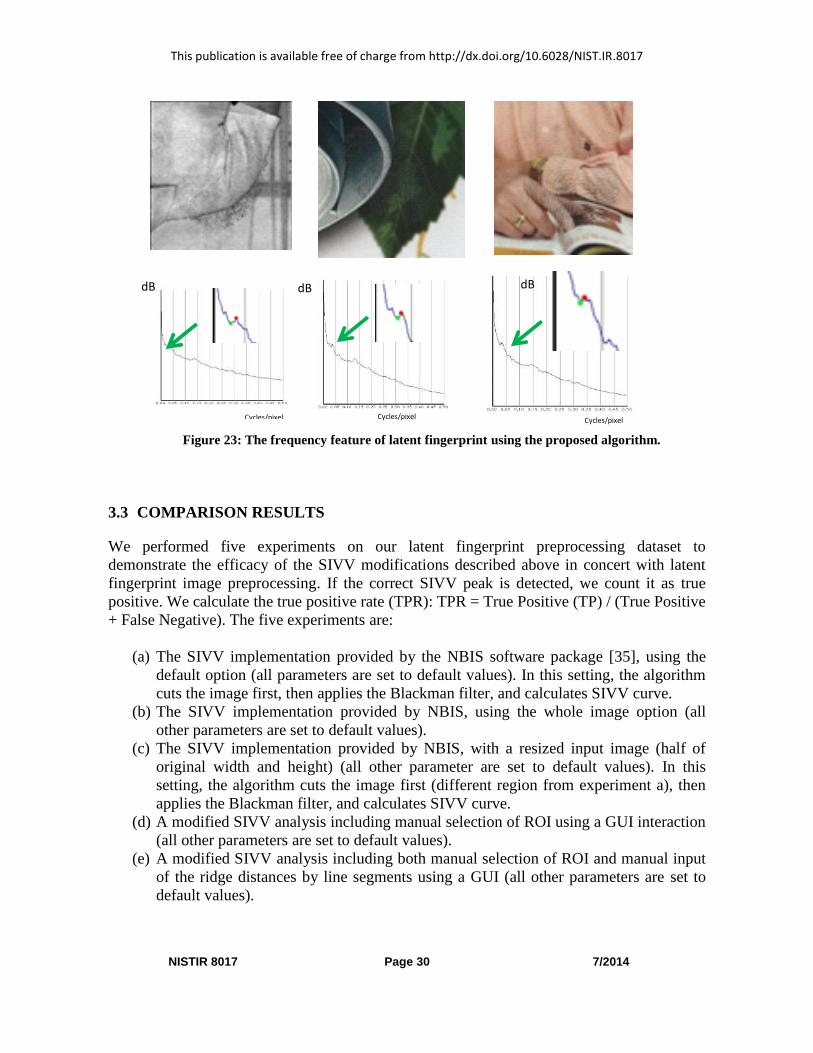
Figure 23 shows the correct peaks are detected using peak location constraints in different
latent fingerprint images.
1. Original image (037 enhanced) 2. Selected ROI 3. Specify ridge distances (max, min)
4. SIVV result Figure 22: Proposed procedure for latent fingerprint SIVV feature detection.
This publication is available free of charge from http://dx.doi.org/10.6028/NIST.IR.8017
NISTIR 8017 Page 30 7/2014
3.3 COMPARISON RESULTS
We performed five experiments on our latent fingerprint preprocessing dataset to
demonstrate the efficacy of the SIVV modifications described above in concert with latent
fingerprint image preprocessing. If the correct SIVV peak is detected, we count it as true
positive. We calculate the true positive rate (TPR): TPR = True Positive (TP) / (True Positive
+ False Negative). The five experiments are:
(a) The SIVV implementation provided by the NBIS software package [35], using the
default option (all parameters are set to default values). In this setting, the algorithm
cuts the image first, then applies the Blackman filter, and calculates SIVV curve.
(b) The SIVV implementation provided by NBIS, using the whole image option (all
other parameters are set to default values).
(c) The SIVV implementation provided by NBIS, with a resized input image (half of
original width and height) (all other parameter are set to default values). In this
setting, the algorithm cuts the image first (different region from experiment a), then
applies the Blackman filter, and calculates SIVV curve.
(d) A modified SIVV analysis including manual selection of ROI using a GUI interaction
(all other parameters are set to default values).
(e) A modified SIVV analysis including both manual selection of ROI and manual input
of the ridge distances by line segments using a GUI (all other parameters are set to
default values).
Figure 23: The frequency feature of latent fingerprint using the proposed algorithm.
dB
Cycles/pixel
dB
Cycles/pixel
dB
Cycles/pixel

This publication is available free of charge from http://dx.doi.org/10.6028/NIST.IR.8017
NISTIR 8017 Page 31 7/2014
The results are shown in Table 1. Clearly the successful detection rates of the preprocessed
images (the values in the second row) are consistently higher than the unprocessed
counterparts (the values in the first row). Based on this, we conclude that preprocessing can
be useful in amplifying fingerprint information contained in latent fingerprint images.
Table 1: The comparison of different algorithms with different options
TPR = TP/(TP+FN)
Original
image
Default
option
Original
image
Whole option
Resize image
Default
option
Original
image
GUI ROI
GUI ROI
Peak loc.
Constraint
Before 36% 33% 62% 79% 85%
After 64% 72% 82% 87% 92%
4 DISCUSSION AND FUTURE WORK
The Spectral Image Validation/Verification (SIVV) analysis was introduced to screen
fingerprint image databases for low-quality and/or non-fingerprint images. It was observed in
that, “The magnitude of the distinctive spectral feature, related directly to the distinctness of
the level 1 ridge flow, provides a primary diagnostic indicator of the presence of a fingerprint
image,” [1]. While effective for controlled capture fingerprints, the diagnostic capability of
SIVV is significantly impaired in the context of low-quality latent fingerprint images. We
have introduced modifications to SIVV to restore this capability. Furthermore, we
demonstrate that the modified SIVV analysis can be used as a quality indicator for
preprocessing, and that it is an essential precursor to detailed forensic investigation of latent
fingerprint images.
This publication is available free of charge from http://dx.doi.org/10.6028/NIST.IR.8017
NISTIR 8017 Page 32 7/2014
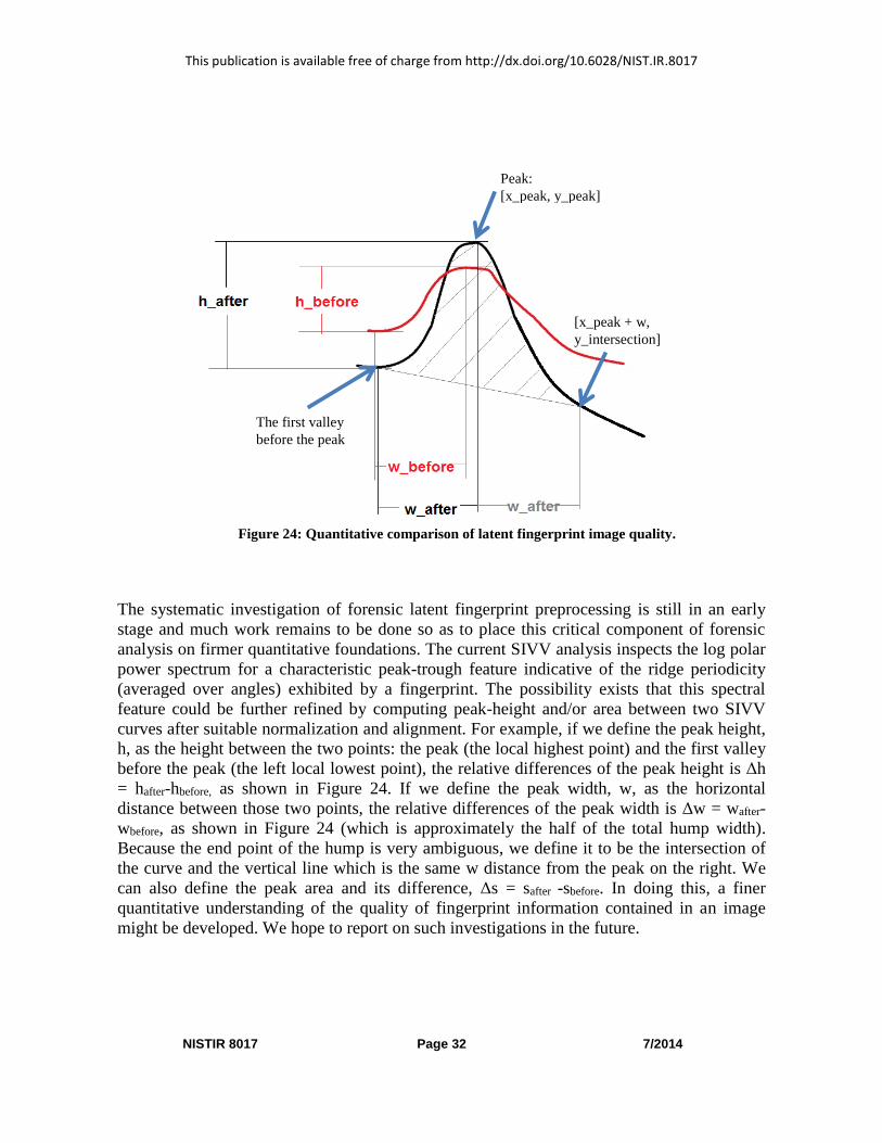
The systematic investigation of forensic latent fingerprint preprocessing is still in an early
stage and much work remains to be done so as to place this critical component of forensic
analysis on firmer quantitative foundations. The current SIVV analysis inspects the log polar
power spectrum for a characteristic peak-trough feature indicative of the ridge periodicity
(averaged over angles) exhibited by a fingerprint. The possibility exists that this spectral
feature could be further refined by computing peak-height and/or area between two SIVV
curves after suitable normalization and alignment. For example, if we define the peak height,
h, as the height between the two points: the peak (the local highest point) and the first valley
before the peak (the left local lowest point), the relative differences of the peak height is Δh
= hafter-hbefore, as shown in Figure 24. If we define the peak width, w, as the horizontal
distance between those two points, the relative differences of the peak width is Δw = wafter-
wbefore, as shown in Figure 24 (which is approximately the half of the total hump width).
Because the end point of the hump is very ambiguous, we define it to be the intersection of
the curve and the vertical line which is the same w distance from the peak on the right. We
can also define the peak area and its difference, Δs = safter -sbefore. In doing this, a finer
quantitative understanding of the quality of fingerprint information contained in an image
might be developed. We hope to report on such investigations in the future.
Figure 24: Quantitative comparison of latent fingerprint image quality.
The first valley
before the peak
Peak:
[x_peak, y_peak]
[x_peak + w,
y_intersection]

This publication is available free of charge from http://dx.doi.org/10.6028/NIST.IR.8017
NISTIR 8017 Page 33 7/2014
5 ACKNOWLEDGEMENTS
The authors thank John M. Libert, John Grantham, and Shahram Orandi of NIST for their
valuable contributions to this work. The authors thank Mathew Schwarz of Schwarz
Forensics and David Witzke of Foray Technologies for valuable consultation on this work.
This research was supported by the 2012 NIST Forensic Measurement Challenges grant,
“Metrics for Manipulation and Enhancement of Forensic Images.”
6 DISCLAIMER
Any mention of commercial products or reference to commercial organizations in this report
is for information only; it does not imply recommendation or endorsement by NIST nor does
it imply that the products mentioned are necessarily the best available for the purpose.
7 REFERENCES
[1] John M. Libert, John Grantham, and Shahram Orandi, “A 1D spectral image
validation/verification metric for fingerprints,” NISTIR 7599, 2009.
[2] Edward M. Robinson, second edition, Crime scene photography. Chapter 10, Digital
Imaging Technologies, contributions by David “Ski” Witzke, Academic Press, 2010.
[3] Andrew M. Dienstfrey, et al., “Analysis of Image Enhancement Operations Applied to
Latent Fingerprints,” NIST IR, Gaithersburg, MD, 2014.
[4] Peter Bajcsy, Joe Chalfoun, David A. Nimorwicz, and Andrew M. Dienstfrey,
“Estimation of Mathematical Models Relating Latent Fingerprint Images Before and
After Enhancement,” NIST IR, Gaithersburg, MD, 2013.
[5] Mary Theofanos, Brian Stanton, et al., “Characterizing the Latent Fingerprint Pre-
processing Procedures,” NIST IR, Gaithersburg, MD, 2014.
[6] David Nimorwicz, Joe Chalfoun, and Peter Bajcsy, “Comparison Metrics for Latent
Fingerprint Images Before and After Enhancement,” NIST IR, Gaithersburg, MD, 2013
This publication is available free of charge from http://dx.doi.org/10.6028/NIST.IR.8017
NISTIR 8017 Page 34 7/2014
[7] Alfred S. Carasso, Alternative Methods of Latent Fingerprint Enhancement and Metrics
for Comparing Them, NISTIR 7910, 2013.
[8] Alfred S. Carasso, “The use of ‘slow motion’ Levy Stable Fractional Diffusion
Smoothing in Alternative Methods of Latent Fingerprint Enhancement,” NISTIR 7932,
2013.
[9] NIST Special Database 27, “Fingerprint Minutiae from Latent and Matching Tenprint
Images,” http://www.nist.gov/srd/nistsd27.cfm.
[10] Michael D. Indovina, V. N. Dvornychenko, E. Tabasse, G. Quinn, P. Grother, M.
Garris, and S. Meagher, “ELFT Phase II: An Evaluation of Automated Latent Fingerprint
Identification Technologies,” U.S. Department of Commerce, National Institute of
Standards and Technology, 2009.
[11] Robert Yen and Joseph Guzman. “Fingerprint image quality measurement
algorithm,” Journal of Forensic Identification 57, no. 2, pp. 274, 2007.
[12] Julian Fierrez-Aguilar, Yi Chen, Javier Ortega-Garcia, and Anil Jain, “Incorporating
image quality in multi-algorithm fingerprint verification,” Advances in Biometrics, pp
213-220, 2005.
[13] Soweon Yoon, Jianjiang Feng, and Anil K. Jain. “On latent fingerprint
enhancement,” SPIE Defense, Security, and Sensing, International Society for Optics and
Photonics, 2010.
[14] Soweon Yoon, Eryun Liu, and Anil K. Jain. “On latent fingerprint image quality,” In
Proc. International Workshop on Computational Forensics. 2012.
[15] Soweon Yoon, Kai Cao, Eryun Liu, and Anil K. Jain, “LFIQ: Latent fingerprint
image quality,” 2013 IEEE Sixth International Conference on Biometrics: Theory,
Applications and Systems (BTAS), pp. 1-8. IEEE, 2013.
[16] M. A. U. Khan, “Fourier cleaning of fingerprint images,” 2010 IEEE 10th
International Conference on Signal Processing (ICSP), pp. 2604-2607. IEEE, 2010.
[17] B. G. Sherlock, D. M. Monro, and K. Millard, “Fingerprint enhancement by
directional Fourier filtering,” IEE Proceedings Vision, Image and Signal Processing, vol.
141, no. 2, pp. 87-94. IET, 1994.

This publication is available free of charge from http://dx.doi.org/10.6028/NIST.IR.8017
NISTIR 8017 Page 35 7/2014
[18] R.T Moore, “An analysis of ridge-to-ridge distance on fingerprints,” J. Forensic
Identification, vol. 39, pp. 231–238, 1989.
[19] Michael D. Garris, and R. Michael McCabe, “NIST Special Database 27: Fingerprint
minutiae from latent and matching tenprint images,” NIST, Gaithersburg, MD. [CD-
ROM] NISTIR 6534.
[20] NIST Biometric Image Software, http://www.nist.gov/itl/iad/ig/nbis.cfm, NIST USA.
[21] Michael W. Reidling, “Recording and Using Photoshop Actions to Streamline
Workflow in Latent Enhancement and Crime Scene Photography,” Presented at the
International Association for Identification's 97th International Educational Conference
on 24 July 2012. http://onin.com/fp/.
[22] Scott Hecker Gische, Glenn Langenburg, and Alice Maceo, “SWGFAST Response to
The Research, Development, Testing & Evaluation Inter-Agency Working Group of the
National Science and Technology Council, Committee on Science, Subcommittee on
Forensic Science,” 2011.
[23] H. Edwards, and C. Gotsonis, “Strengthening forensic science in the United States: a
path forward,” Statement before the United State Senate Committee on the Judiciary.
Chapter 10, Automated Fingerprint Identification Systems, 2009.
[24] John C. Russ, “Forensic uses of digital imaging,” CRC, pp. 549, 2001.
[25] Bramble, Simon, David Compton, and L. Klasén, “Forensic image analysis,” In Proc.
of 13th INTERPOL Forensic Science Symposium, Lyon FR. 2001.
[26] A. Hicklin, and C. Reedy, “Implications of the IDENT/IAFIS Image Quality Study
for Visa Fingerprint Processing,” Mitertek Systems (MTS), 2002.
[27] Tai Pang Chen, Xudong Jiang, and Wei Yun Yau, “Fingerprint image quality
analysis,” 2004 International Conference on Image Processing (ICIP'04). Vol. 2. IEEE,
2004.
[28] Yi Chen, Sarat Dass, and Anil Jain, “Fingerprint quality indices for predicting
authentication performance,” In Audio-and Video-Based Biometric Person
Authentication, pp. 160-170. Springer Berlin/Heidelberg, 2005.

This publication is available free of charge from http://dx.doi.org/10.6028/NIST.IR.8017
NISTIR 8017 Page 36 7/2014
[29] Elham Tabassi, Charles L. Wilson, and Craig I. Watson. Fingerprint image quality.
U.S. Department of Commerce, National Institute of Standards and Technology, 2004.
[30] Jacqueline A. Speir, Jack Hietpas, Tara Fikes, “Fast Fourier transformation and
frequency filtering to suppress background noise in fingerprint evidence: quantifying the
fidelity of digitally enhanced fingerprint evidence,” Cedar Crest College, Allentown PA,
Syracuse Univ., Syracuse, NY.
[31] Bradford T. Ulery, R. Austin Hicklin, JoAnn Buscaglia, and Maria Antonia Roberts,
“Accuracy and reliability of forensic latent fingerprint decisions,” Proceedings of the
National Academy of Sciences 108, no. 19, pp. 7733-7738, 2011.
[32] Sargur N. Srihari and Graham Leedham, “A survey of computer methods in forensic
document examination,” In Proceedings of the 11th Conference of the International
Graphonomics Society, pp. 279. 2003.
[33] Matthew Stamm and KJ Ray Liu, “Blind forensics of contrast enhancement in digital
images,” 15th IEEE International Conference on Image Processing (ICIP’08), pp. 3112-
3115, IEEE, 2008.
[34] Foray, “calibrating your images,”
http://www.foray.com/images/pdfs/CalibratingYourImages.pdf.
[35] Flynn Mcroberts and Steve Mills, Chicago Tribune, “FBI's digital fingerprints could
collar the innocent,” http://articles.dailypress.com/2005-01-
04/news/0501040066_1_inked-print-cards-prominent-fingerprint-latent-prints-training-
coordinator, January 04, 2005.
[36] Chicago Tribune, “Digital fingerprint technology can point to wrong person,” The
Baltimore Sun, http://articles.baltimoresun.com/2005-01-
30/news/0501290073_1_digital-image-digital-fingerprint-computer-images, January 30,
2005.
[37] Photo Finish, online document, www.fdiai.org/articles/Photo%20Finish.pdf.
This publication is available free of charge from http://dx.doi.org/10.6028/NIST.IR.8017
NISTIR 8017 Page 37 7/2014
APPENDIX A: THE SIVV PEAK ON SYNTHETIC IMAGES
In order to study the properties of SIVV and find out the relationship between the SIVV peak
location and texture frequencies, we generated a set of synthetic images. The first image set
is a set of black/white stripe images with different stripe width. The size of the images in the
first image set is 512 by 512. For each image, given the width of the stripes, we generate the
image with black/white stripes with equal width. Figure 25 shows the comparisons of SIVV
peaks of images with the different stripe width. Table 2 shows the stripe width and their
SIVV peak location. In the frequency range of the texture pattern that we consider,5 the peak
location follows a certain rule. Generally, the narrow stripe image’s SIVV peak location is
smaller (or closer to the origin) than the wide stripe image’s peak location for the same
texture pattern.
The size each image in the second image set is 1024 by 1024 in Figure 26. Similarly as the
experiment on the first image set, given the width of the stripes, the images are synthesized
and their frequency feature are extracted. Table 3 shows the stripe width and their SIVV peak
locations. Comparing Table 2 and Table 3, firstly, it indicates that the peak location is not
related to the image size. It is reasonable because the x-axis of the SIVV curve is the cycles
per pixel. The x-axis is normalized by the image size in the last step of SIVV algorithm.
Secondly, the SIVV peak location is related with the width of the stripe directly. For
example, the peak location of the image with four-pixel stripe width is 0.25 for both image
with the size of 512 by 512 and the image with the size of 1024 by 1024. The peak location
is 0.125 of the images with eight-pixel stripe width for both image sizes. For the same texture
pattern (as our stripe pattern example), the peak location is decided by the pixel distance of
the pattern width. The peak location follows the same rule as the first set: the SIVV peak
location of the image with the narrow stripe is closer to the origin than the one of the image
with wide stripe.
On the other hand, notice that the image B in Set 2 (resolution: 1024×1024; stripe width: 8
pixels) is just the high-resolution version of the image A in Set 1 (resolution: 512×512; stripe
width: 4 pixels). If we resample image B in Set 2 by taking every other pixel in both column
and row, we obtain the image A in Set 1. PPI (Pixels Per Inch) of the first image (the image
B in Set 2) is twice as the second image (the image A in Set 1). In our case, if we scan the
same forensic latent fingerprint with different PPI, the peak location of high PPI (B in set 2)
5 We study the texture patterns in a certain frequency range. If the frequency is too high (i.e., the stripe width is 1 or 2
pixels for the image with size 512×512, SIVV curve does not show peaks. If the frequency is too low, SIVV shows
peaks in multiple locations (like a wave). In our study, we consider only the frequency in a certain range, which is
relatively high compared with the image size. No extreme case is considered here.

This publication is available free of charge from http://dx.doi.org/10.6028/NIST.IR.8017
NISTIR 8017 Page 38 7/2014
is half of the peak location of low PPI image (A in Set 1). Table 4 shows the comparison
results.
In summary, the SIVV peak location is directly related to the stripe width in pixel distance.
Table 5 shows the peak location given the stripe width. We may use it as a reference for the
proposed peak location constraint algorithm.
Finally, we also generate another set of synthetic image with square pattern (as shown in
Figure 27). It shows that SIVV peak location follows the same rule; just the location of the
peak is different given different texture pattern.

This publication is available free of charge from http://dx.doi.org/10.6028/NIST.IR.8017
NISTIR 8017 Page 39 7/2014
Set 1 B-1. width: 8 (512×512)
Set 1 A-1. width: 4 (512×512)
Set 1 C-1. width: 16 (512×512)
Set 1 D-1. width: 32 (512×512)
A-2. 2D DFT power spectrum (4)
B-2. 2D DFT power spectrum (8)
C-2. 2D DFT power spectrum (16)
D-2. 2D DFT power spectrum (32)
A-3. 2D Polar spectrum (4)
B-3. 2D Polar spectrum (8)
C-3. 2D Polar spectrum (16)
D-3. 2D Polar spectrum (32)
A-4. SIVV (4)
B-4. SIVV (8)
C-4. SIVV (16)
Figure 25: SIVV on the images with the stripes pattern (image size 512×512 pixels).
D-4. SIVV (32)

This publication is available free of charge from http://dx.doi.org/10.6028/NIST.IR.8017
NISTIR 8017 Page 40 7/2014
Table 2: SIVV peak locations on the images with the stripes pattern (image size 512×512 pixels)
Stripe width 4 8 16 32
Set 2 B-1. width: 8 (1024 ×1024)
Set 2 A-1. width: 4 (1024 ×1024)
Set 2 C-1. width: 16 (1024 ×1024)
Set 2 D-1. width: 32 (1024 ×1024)
A-2. 2D DFT power spectrum (4)
B-2. 2D DFT power spectrum (8)
C-2. 2D DFT power spectrum (16)
D-2. 2D DFT power spectrum (32)
A-3. 2D Polar spectrum (4)
B-3. 2D Polar spectrum (8)
C-3. 2D Polar spectrum (16)
D-3. 2D Polar spectrum (32)
A-4. SIVV (4; location 0.25)
B-4. SIVV (8; location 0.125)
C-4. SIVV (16; location 0.0625)
D-4. SIVV (32; location 0.312)
Figure 26: SIVV on the large images with the stripes pattern (image size 1024×1024 pixels).

This publication is available free of charge from http://dx.doi.org/10.6028/NIST.IR.8017
NISTIR 8017 Page 41 7/2014
Peak location 0.25 0.125 0.625 0.312
Table 3: SIVV peak locations on the large images with the stripes pattern (image size 1024×1024 pixels)
Stripe width 4 8 16 32
Peak location 0.25 0.125 0.625 0.312
Table 4: The relationship between peak locations and PPI
512×512 Strip width 4 8 16 512×512 Peak location 0.25 0.125 0.625
Double PPI of first row
(the image looks the
same, but the resolution
is doubled in both x, and
y directions)
1024×1024 strip width 8 16 32 1024×1024 peak location 0.125 0.0625 0.0312
Table 5: The peak locations given the stripe pixel distance.
4 8 12 16 20 24 28 32 36 40
0.25 0.125 0.083 0.0625 0.05 0.042 0.035 0.031 0.027 0.025

This publication is available free of charge from http://dx.doi.org/10.6028/NIST.IR.8017
NISTIR 8017 Page 42 7/2014
B. width: 8 (512×512)
A. width: 4 (512×512) C. width: 16 (512×512)
D. width: 32 (512×512)
A-4. SIVV (4; location 0.35) B-4. SIVV (8; location 0.175) C-4. SIVV (16; location:0.085)
D-4. SIVV (32; Around 0.04)
Figure 27: SIVV on the images with square pattern.