a measurement of the top quark mass in the dilepton decay ...a measurement of the top quark mass in...
TRANSCRIPT

A Measurement of the Top Quark Mass in the
Dilepton Decay Channel at CDF II
by
Bodhitha A. Jayatilaka
A dissertation submitted in partial fulfillmentof the requirements for the degree of
Doctor of Philosophy(Physics)
in The University of Michigan2006
Doctoral Committee:
Associate Professor David W. Gerdes, ChairProfessor Mario L. MateoProfessor Timothy A. McKayProfessor Jianming QianAssociate Professor James T. Liu

c© Bodhitha A. Jayatilaka 2006All Rights Reserved

DEDICATION
To Amma and Thaththa.
ii

ACKNOWLEDGEMENTS
There are many people who helped make this work possible and who I am honored to
have worked with and know.
My advisor Dave Gerdes, who proposed such an interesting research topic and who
stood by me in difficult circumstances. Monica Tecchio, who was never hesitant to share
with me her vast expanse of knowledge. I’ve also been lucky to work with our collaborators
from Penn who are some of the smartest and most talented physicists I know. Daniel
Whiteson, who drove this analysis effort from day one and was always willing to offer
advice, even if not about physics. Andrew Kovalev, who laid so much groundwork and
led by example with his mathematical rigor. And Brig Williams for advice and invaluable
words of encouragement.
Many people help make the Michigan CDF group feel more like family than anything
else. The faculty: Dan Amidei, who not only ran a tight ship, but also was always there
to share advice and his enthusiasm for physics; and Myron Campbell, who showed great
trust in giving me the opportunity to get my feet wet in the electronics shop. My former
housemates: Kathy Copic, Clark Cully, Nate Goldschmidt and Mitch Soderberg, who
helped make living on-site bearable. And everyone else in the group during my time with
it who offered advice, assistance and camaraderie: Ken Bloom, Claudio Ferretti, Stephen
Miller, Fred Niell, Tom Schwarz, Tom Wright and Alexei Varganov.
The top group and top mass group conveners at CDF helped bring this analysis, in
iii

its many incarnations, to fruition: Robin Erbacher, Taka Murayama, Evelyn Thomson,
Florencia Cannelli, Doug Glenzinksi, and Un-Ki Yan. Our “godparent committee” worked
tirelessly to help bring not one but two publications to completion: Jay Hauser, Jeremy
Lys and Markus Klute.
My dissertation committee members who, despite being given such short notice, were
willing give me some of their valuable time: Jim Liu, Tim McKay, Mario Mateo and
Jianming Qian.
There are faculty at UC Berkeley and staff at LBNL who really helped steer me into
this field and to whom I am indebted for it: Sandra Ciocio, Bob Jacobsen, Marjorie
Shapiro, Mark Strovink, and Jim Siegrist.
Back in Ann Arbor, the “physics cronies” (too many names to list here– but you know
who you are) helped show that graduate school can be a place to have fun and to make
great friends.
My parents and my brother, whose love and support were there from the beginning.
And last, but far from least, Alana Kirby, whose love, support, and encouragement
could always be counted on and never went unnoticed.
iv

TABLE OF CONTENTS
DEDICATION . . . . . . . . . . . . . . . . . . . . . . . . . . . . . . . . . . . . . . . . . . . . . . ii
ACKNOWLEDGEMENTS . . . . . . . . . . . . . . . . . . . . . . . . . . . . . . . . . . . . . . iii
LIST OF FIGURES . . . . . . . . . . . . . . . . . . . . . . . . . . . . . . . . . . . . . . . . . . viii
LIST OF TABLES . . . . . . . . . . . . . . . . . . . . . . . . . . . . . . . . . . . . . . . . . . . xiii
ABSTRACT . . . . . . . . . . . . . . . . . . . . . . . . . . . . . . . . . . . . . . . . . . . . . . . xiv
CHAPTER1. Introduction . . . . . . . . . . . . . . . . . . . . . . . . . . . . . . . . . . . . . . . . . . 1
2. The Standard Model and Top Quark Physics . . . . . . . . . . . . . . . . . . . . . 3
2.1 The Standard Model . . . . . . . . . . . . . . . . . . . . . . . . . . . . . . . . . . 32.2 The Top Quark . . . . . . . . . . . . . . . . . . . . . . . . . . . . . . . . . . . . . 5
2.2.1 Top Quark Production . . . . . . . . . . . . . . . . . . . . . . . . . . . . 62.2.2 Top Quark Decay . . . . . . . . . . . . . . . . . . . . . . . . . . . . . . . 7
2.3 Top Quark Mass in the Dilepton Channel . . . . . . . . . . . . . . . . . . . . . . . 9
3. Experimental Apparatus . . . . . . . . . . . . . . . . . . . . . . . . . . . . . . . . . . 13
3.1 The Collider . . . . . . . . . . . . . . . . . . . . . . . . . . . . . . . . . . . . . . . 133.1.1 The Proton Source and Pre-Acceleration . . . . . . . . . . . . . . . . . . 133.1.2 The Antiproton Source . . . . . . . . . . . . . . . . . . . . . . . . . . . . 153.1.3 The Tevatron . . . . . . . . . . . . . . . . . . . . . . . . . . . . . . . . . 16
3.2 The CDF Detector . . . . . . . . . . . . . . . . . . . . . . . . . . . . . . . . . . . 173.2.1 The Tracking System . . . . . . . . . . . . . . . . . . . . . . . . . . . . . 203.2.2 Calorimeters . . . . . . . . . . . . . . . . . . . . . . . . . . . . . . . . . . 233.2.3 The Muon Detector . . . . . . . . . . . . . . . . . . . . . . . . . . . . . . 243.2.4 Trigger System . . . . . . . . . . . . . . . . . . . . . . . . . . . . . . . . 26
4. Data Sample and Event Selection . . . . . . . . . . . . . . . . . . . . . . . . . . . . . 29
4.1 Trigger Requirements . . . . . . . . . . . . . . . . . . . . . . . . . . . . . . . . . . 294.2 Event Selection . . . . . . . . . . . . . . . . . . . . . . . . . . . . . . . . . . . . . 30
4.2.1 Leptons . . . . . . . . . . . . . . . . . . . . . . . . . . . . . . . . . . . . 304.2.2 Jets . . . . . . . . . . . . . . . . . . . . . . . . . . . . . . . . . . . . . . 314.2.3 Final Selection Cuts . . . . . . . . . . . . . . . . . . . . . . . . . . . . . 33
4.3 Backgrounds . . . . . . . . . . . . . . . . . . . . . . . . . . . . . . . . . . . . . . . 344.4 Sample Composition . . . . . . . . . . . . . . . . . . . . . . . . . . . . . . . . . . 35
v

5. Method Overview . . . . . . . . . . . . . . . . . . . . . . . . . . . . . . . . . . . . . . . 38
5.1 Signal Likelihood . . . . . . . . . . . . . . . . . . . . . . . . . . . . . . . . . . . . 395.2 Accounting for Background Processes . . . . . . . . . . . . . . . . . . . . . . . . . 42
6. Transfer Functions . . . . . . . . . . . . . . . . . . . . . . . . . . . . . . . . . . . . . . 43
6.1 Jet Transfer Functions . . . . . . . . . . . . . . . . . . . . . . . . . . . . . . . . . 436.2 tt pT Transfer Functions . . . . . . . . . . . . . . . . . . . . . . . . . . . . . . . . 48
7. Signal Probability . . . . . . . . . . . . . . . . . . . . . . . . . . . . . . . . . . . . . . . 52
7.1 Differential Cross-Section Expression . . . . . . . . . . . . . . . . . . . . . . . . . 527.2 Phase Space Transformation and Integration . . . . . . . . . . . . . . . . . . . . . 547.3 Tests of the Signal Probability . . . . . . . . . . . . . . . . . . . . . . . . . . . . . 58
7.3.1 Jet-Parton Assignment . . . . . . . . . . . . . . . . . . . . . . . . . . . . 617.3.2 Lepton Resolution . . . . . . . . . . . . . . . . . . . . . . . . . . . . . . 617.3.3 Jet Angle Resolution . . . . . . . . . . . . . . . . . . . . . . . . . . . . . 62
8. Background Probabilities . . . . . . . . . . . . . . . . . . . . . . . . . . . . . . . . . . 64
8.1 Matrix Element Evaluation . . . . . . . . . . . . . . . . . . . . . . . . . . . . . . . 648.2 Z/γ∗ + 2 jets . . . . . . . . . . . . . . . . . . . . . . . . . . . . . . . . . . . . . . 658.3 WW + 2 jets . . . . . . . . . . . . . . . . . . . . . . . . . . . . . . . . . . . . . . . 688.4 Fakes . . . . . . . . . . . . . . . . . . . . . . . . . . . . . . . . . . . . . . . . . . . 69
9. Mass Extraction and Calibration . . . . . . . . . . . . . . . . . . . . . . . . . . . . . 73
9.1 Mass Extraction . . . . . . . . . . . . . . . . . . . . . . . . . . . . . . . . . . . . . 739.1.1 Posterior Probability . . . . . . . . . . . . . . . . . . . . . . . . . . . . . 73
9.2 Calibration . . . . . . . . . . . . . . . . . . . . . . . . . . . . . . . . . . . . . . . . 749.2.1 Signal only tests with Ps . . . . . . . . . . . . . . . . . . . . . . . . . . . 759.2.2 Signal and Background tests with Ps . . . . . . . . . . . . . . . . . . . . 759.2.3 Signal and Background tests with Ps and Pb . . . . . . . . . . . . . . . . 76
10. Systematic Uncertainties . . . . . . . . . . . . . . . . . . . . . . . . . . . . . . . . . . 81
10.1 Jet Energy Scale . . . . . . . . . . . . . . . . . . . . . . . . . . . . . . . . . . . . . 8110.2 Generator . . . . . . . . . . . . . . . . . . . . . . . . . . . . . . . . . . . . . . . . 8210.3 Response calibration . . . . . . . . . . . . . . . . . . . . . . . . . . . . . . . . . . 8210.4 Sample composition . . . . . . . . . . . . . . . . . . . . . . . . . . . . . . . . . . . 8310.5 PDF uncertainties and αs . . . . . . . . . . . . . . . . . . . . . . . . . . . . . . . 8410.6 Radiation . . . . . . . . . . . . . . . . . . . . . . . . . . . . . . . . . . . . . . . . . 8510.7 Background statistics . . . . . . . . . . . . . . . . . . . . . . . . . . . . . . . . . . 8610.8 Background Modeling . . . . . . . . . . . . . . . . . . . . . . . . . . . . . . . . . . 86
10.8.1 Drell-Yan . . . . . . . . . . . . . . . . . . . . . . . . . . . . . . . . . . . 8610.8.2 Fake background . . . . . . . . . . . . . . . . . . . . . . . . . . . . . . . 88
10.9 Lepton Energy Scale . . . . . . . . . . . . . . . . . . . . . . . . . . . . . . . . . . 8910.10Summary . . . . . . . . . . . . . . . . . . . . . . . . . . . . . . . . . . . . . . . . . 90
11. Measurement in Data . . . . . . . . . . . . . . . . . . . . . . . . . . . . . . . . . . . . 91
11.1 Kinematic Properties of Observed Events . . . . . . . . . . . . . . . . . . . . . . . 91
vi

11.2 Result . . . . . . . . . . . . . . . . . . . . . . . . . . . . . . . . . . . . . . . . . . . 94
12. Conclusion . . . . . . . . . . . . . . . . . . . . . . . . . . . . . . . . . . . . . . . . . . . 100
APPENDIX A . . . . . . . . . . . . . . . . . . . . . . . . . . . . . . . . . . . . . . . . . . . . . . 103
BIBLIOGRAPHY . . . . . . . . . . . . . . . . . . . . . . . . . . . . . . . . . . . . . . . . . . . . 112
vii

LIST OF FIGURES
Figure
2.1 Corrections to the W boson observed mass via loop diagrams. Left : A fermion loopinvolving top and bottom quarks. The large top quark mass dominates this correction,which is proportional to M2
t . Right : A Higgs boson loop which contributes a correctionproportional to ln MH . . . . . . . . . . . . . . . . . . . . . . . . . . . . . . . . . . . . . . 5
2.2 Left : Constraints on the standard model Higgs boson mass as a function of top quarkmass and W boson mass as of March 2006. The red curve shows the 68% CL constraintobtained from studies at the Z pole made at SLD and LEP. The dashed blue curveshows the 68% CL constraint obtained from direct measurements of MW and Mt madeat LEP and the Tevatron. Right : The ∆χ2 (black curve) to a global fit of standardmodel parameters to a standard model Higgs boson mass. The yellow band shows theregion excluded by direct searches at LEP. Courtesy of the LEP Electroweak WorkingGroup [11]. . . . . . . . . . . . . . . . . . . . . . . . . . . . . . . . . . . . . . . . . . . . 6
2.3 Top: Leading-order production diagram for qq → tt. Bottom: Leading-order productiondiagrams for gg → tt. . . . . . . . . . . . . . . . . . . . . . . . . . . . . . . . . . . . . . . 7
2.4 NLO calculations of σtt [15] for pp collisions at√
s = 1.96 TeV as a function of Mt. Alsoshown are experimental measurements of σtt made at CDF using Run II [16] data. . . . 8
2.5 Decay of tt in the dilepton channel. . . . . . . . . . . . . . . . . . . . . . . . . . . . . . . 10
2.6 World average of the top quark mass along with the individual measurements used tocalculate it as of March 2006 [18]. . . . . . . . . . . . . . . . . . . . . . . . . . . . . . . . 12
3.1 A schematic view of the Fermilab accelerator complex. Figure courtesy of FermilabAccelerator Division. . . . . . . . . . . . . . . . . . . . . . . . . . . . . . . . . . . . . . . 14
3.2 The total integrated luminosity at CDF as of February 2006. The red curve showsthe total integrated luminosity delivered to CDF while the blue curve shows the totalintegrated luminosity written to tape at CDF. . . . . . . . . . . . . . . . . . . . . . . . . 18
3.3 A cross-sectional view of the CDF detector [19]. . . . . . . . . . . . . . . . . . . . . . . . 19
3.4 A schematic overview of the CDF tracking system. The region of the detector with|η| < 1.0 is referred to as the “central” region. . . . . . . . . . . . . . . . . . . . . . . . . 21
3.5 The SVX barrel structure [19]. . . . . . . . . . . . . . . . . . . . . . . . . . . . . . . . . 22
3.6 Coverage of the CDF muon systems. . . . . . . . . . . . . . . . . . . . . . . . . . . . . . 25
3.7 The CDF Trigger and Data Acquisition System. . . . . . . . . . . . . . . . . . . . . . . . 27
viii
4.1 pjetT /pγ
T − 1 in γ+jets events as a function of η of the jets after relative corrections areapplied. Response is seen to be nearly flat for data as well as for events simulated withPythia [33] or Herwig [34]. . . . . . . . . . . . . . . . . . . . . . . . . . . . . . . . . . 32
4.2 The predicted jet multiplicity of events in the DIL selection with that observed in thedata overlaid. The first three bins contain events that have not had the HT and oppositesign cut applied to them while the final bin contains events passing all selection cutsoutlined in this chapter. . . . . . . . . . . . . . . . . . . . . . . . . . . . . . . . . . . . . 36
4.3 The Acceptance of the DIL selection criteria as a function of top quark mass. The sampleof simulated event used is generated using the Herwig generator [34] and includes ttdecays to all standard model decay channels with the theoretically predicted branchingratios. The parameterization shown is for a fit to the function A = p0 + p1Mt + p2M
2t . . 37
6.1 Top, difference of Ep − Ej between parton and jet energy. Center, distribution of Ej ofjet energy. Bottom, input distribution of parton energy Ep. Histograms are simulatedevents for Mt = 178 GeV/c2; curves in the upper two histograms show the distributionscalculated using W (Ep, Ej). . . . . . . . . . . . . . . . . . . . . . . . . . . . . . . . . . . 46
6.2 Comparison of simulated Ej with calculations from W (Ep, Ej) from six ranges of Ep.Histograms are simulated events; curves show the calculated distributions using W (Ep, Ej). 47
6.3 Comparison of simulated Ej with calculations from W (Ep, Ej) from distributions Ep insimulated samples with Mt = 150, 160, 170, 180, 190, and 200 GeV/c2. Histogramsare simulated events for Mt = 178 GeV/c2; lines show the calculated distributions usingWj(Ep, Ej) derived using partons from Mt = 178 GeV/c2. . . . . . . . . . . . . . . . . . 47
6.4 Mean pttT for Pythia simulated tt events with the number of reconstructed jets ranging
from two to seven or more. . . . . . . . . . . . . . . . . . . . . . . . . . . . . . . . . . . 49
6.5 The distributions of δpTfor events with more than two jets (right) and exactly two jets
(left). The extracted fits are overlaid with the individual Gaussians in black and the totalfit in red. . . . . . . . . . . . . . . . . . . . . . . . . . . . . . . . . . . . . . . . . . . . . 50
6.6 The distributions of δφ for events with more than two jets (right) and exactly two jets(left). The extracted fits are overlaid in red. . . . . . . . . . . . . . . . . . . . . . . . . . 51
7.1 A plot of the difference between the true neutrino energy and neutrino energy as solvedfrom equation 7.6 in simulated events using parton-level quantities. . . . . . . . . . . . . 56
7.2 Evaluation of the tt matrix element using parton-level information from Monte Carloevents. . . . . . . . . . . . . . . . . . . . . . . . . . . . . . . . . . . . . . . . . . . . . . . 59
7.3 Evaluation of Ps using Monte Carlo events with smeared partons. . . . . . . . . . . . . . 60
7.4 Angular distance, ∆R, between a reconstructed jet and the closest b-quark in tt eventssimulated with herwig. The width of the distribution demonstrates the angular reso-lution. 20% of jet-parton pairs have ∆R ≥ 0.7 (not shown), coming from jets with nocorresponding b-quark. . . . . . . . . . . . . . . . . . . . . . . . . . . . . . . . . . . . . . 62
8.1 Variation in log(|M |2) with increasing number of terms in the spin and color sum. Fromtop, moving downwards, the number of spin terms sampled increases by powers of 2 from1 to 32. From left, moving right, the number of color terms sampled increases by powersof 2 from 1 to 32. . . . . . . . . . . . . . . . . . . . . . . . . . . . . . . . . . . . . . . . 66
ix
8.2 Variation of the squared matrix element for pp → Z(→ ll) + 2 jets as a function of theleptonic pair invariant mass. . . . . . . . . . . . . . . . . . . . . . . . . . . . . . . . . . 67
8.3 Evaluation of the Zjj probability for fully reconstructed Z and tt events, after selectionis applied. . . . . . . . . . . . . . . . . . . . . . . . . . . . . . . . . . . . . . . . . . . . 68
8.4 Left: Evaluation of the squared matrix element for pp → WW (→ lνlν) + 2 jets forparton-level tt and WW + 2p events. Right: Evaluation of the WWjj probability forWW and tt events in fully simulated events, after selection has been applied. . . . . . . 70
8.5 Left: Evaluation of the squared matrix element for pp → W (→ lν)+3 jets for parton-leveltt and W + 3p events. Right: Evaluation of the Wjjj probability for Gaussian smearedWjjj and tt events. . . . . . . . . . . . . . . . . . . . . . . . . . . . . . . . . . . . . . . 71
8.6 Evaluation of the Wjjj probability for fully simulated tt and events from the data whichare candidates to produce a fake lepton. . . . . . . . . . . . . . . . . . . . . . . . . . . . 72
9.1 Response for Monte Carlo experiments of signal events, using only Ps to extract the mass. 76
9.2 Residual in top mass, and mean of pull distribution for varying simulated Mt, in signal-only Monte Carlo experiments. . . . . . . . . . . . . . . . . . . . . . . . . . . . . . . . . 76
9.3 Response for Monte Carlo experiments of signal and background events, using only Ps
to extract the mass. . . . . . . . . . . . . . . . . . . . . . . . . . . . . . . . . . . . . . . 77
9.4 Response for Monte Carlo experiments of signal and background events, using only Ps
to extract the mass. . . . . . . . . . . . . . . . . . . . . . . . . . . . . . . . . . . . . . . 78
9.5 Residual in top mass, and mean of pull distribution for varying simulated Mt, in MonteCarlo experiments including both signal and background events. The probability expres-sion includes both Ps and Pb. . . . . . . . . . . . . . . . . . . . . . . . . . . . . . . . . . 79
9.6 Residual in top mass, and mean of pull distribution for varying simulated Mt, MonteCarlo experiments after error scaling. . . . . . . . . . . . . . . . . . . . . . . . . . . . . . 79
9.7 Distribution of measured mass, measured statistical error, and pulls for pseudo-experimentsusing signal events of Mt = 175 GeV/c2 and expected numbers of background events. . . 79
9.8 Distribution of measured mass, measured statistical error, and pulls for pseudo-experimentsusing signal events of Mt = 165 GeV/c2 and expected numbers of background events. . . 80
10.1 Difference in extracted mass between the positive and negative PDF eigenvectors for aPythia sample. . . . . . . . . . . . . . . . . . . . . . . . . . . . . . . . . . . . . . . . . . 84
10.2 Variation in measured mass when background samples are split into disjoint sets. Topleft, Z; Top right, Fakes. Middle left, WW ; Middle right, WZ. Bottom, Z → ττ . . . . . 87
11.1 Comparison of the tt probability distribution for simulated events, scaled by expectedcontribution to the sample composition, to that for observed events. . . . . . . . . . . . 92
11.2 Comparison of the Zjj probability distribution for simulated events, scaled by expectedcontribution to the sample composition, to that for observed events. . . . . . . . . . . . 92
11.3 Comparison of the WWjj probability distribution for simulated events, scaled by ex-pected contribution to the sample composition, to that for observed events. . . . . . . . 93
x

11.4 Comparison of the Fake probability distribution for simulated events, scaled by expectedcontribution to the sample composition, to that for observed events. . . . . . . . . . . . 93
11.5 Posterior probabilities for each of the 33 candidate events found in 340 pb−1 of datacollected between March 2002 and August 2004. Each includes the normalized signaland background probabilities. . . . . . . . . . . . . . . . . . . . . . . . . . . . . . . . . . 95
11.6 Posterior probabilities for each of the 31 candidate events found in the 400 pb−1 of datacollected between December 2004 and September 2005. Each includes the normalizedsignal and background probabilities. . . . . . . . . . . . . . . . . . . . . . . . . . . . . . 96
11.7 Posterior probabilities for each of the 14 candidate events found in the 260 pb−1 of datacollected between September 2005 and February 2006. Each includes the normalizedsignal and background probabilities. . . . . . . . . . . . . . . . . . . . . . . . . . . . . . 97
11.8 Final posterior probability density as a function of the top pole mass for the 78 candidateevents in the data. . . . . . . . . . . . . . . . . . . . . . . . . . . . . . . . . . . . . . . . 98
11.9 Distribution of expected errors for Mt = 165 GeV/c2. The measured error is shows asthe line; 46% of pseudo-experiments yield a smaller error. . . . . . . . . . . . . . . . . . 98
11.10 Measurement of the top quark mass in ee, µµ and eµ events separately. The measurementin all data events is also shown for comparison. Only statistical uncertainties are shown. 99
A.1 Transverse momentum (PT ), azimuthal angle (φ) and pseudo-rapidity (η) of the leadingjet. . . . . . . . . . . . . . . . . . . . . . . . . . . . . . . . . . . . . . . . . . . . . . . . . 103
A.2 Transverse momentum (PT ), azimuthal angle (φ) and pseudo-rapidity (η) of the secondjet. . . . . . . . . . . . . . . . . . . . . . . . . . . . . . . . . . . . . . . . . . . . . . . . . 103
A.3 Transverse momentum (PT ), azimuthal angle (φ) and pseudo-rapidity (η) of the third jet. 106
A.4 Transverse momentum (PT ), azimuthal angle (φ) and pseudo-rapidity (η) of the leadinglepton. . . . . . . . . . . . . . . . . . . . . . . . . . . . . . . . . . . . . . . . . . . . . . . 106
A.5 Transverse momentum (PT ), azimuthal angle (φ) and pseudo-rapidity (η) of the secondlepton. . . . . . . . . . . . . . . . . . . . . . . . . . . . . . . . . . . . . . . . . . . . . . . 107
A.6 Transverse momentum (PT ), azimuthal angle (φ) and pseudo-rapidity (η) of the missingtransverse energy. . . . . . . . . . . . . . . . . . . . . . . . . . . . . . . . . . . . . . . . . 107
A.7 Transverse momentum (PT ), azimuthal angle (φ) and pseudo-rapidity (η) of the vectorsum of the leptons. . . . . . . . . . . . . . . . . . . . . . . . . . . . . . . . . . . . . . . . 107
A.8 Difference in transverse momentum (PT ), azimuthal angle (φ) and pseudo-rapidity (η)of the two leptons. . . . . . . . . . . . . . . . . . . . . . . . . . . . . . . . . . . . . . . . 108
A.9 Transverse momentum (PT ), azimuthal angle (φ) and pseudo-rapidity (η) of the vectorsum of the jets. . . . . . . . . . . . . . . . . . . . . . . . . . . . . . . . . . . . . . . . . . 108
A.10 Distribution of HT and Njets. . . . . . . . . . . . . . . . . . . . . . . . . . . . . . . . . . 109
A.11 Distribution of transverse unclustered energy. . . . . . . . . . . . . . . . . . . . . . . . . 110
A.12 Transverse momentum (PT ), azimuthal angle (φ) and pseudo-rapidity (η) of the differencebetween the leading jets. . . . . . . . . . . . . . . . . . . . . . . . . . . . . . . . . . . . 110
xi

A.13 Transverse momentum (PT ), azimuthal angle (φ) and pseudo-rapidity (η) of the differencebetween the missing energy and the leading jet. . . . . . . . . . . . . . . . . . . . . . . . 111
A.14 Transverse momentum (PT ), azimuthal angle (φ) and pseudo-rapidity (η) of the vectorsum of both jets and leptons. . . . . . . . . . . . . . . . . . . . . . . . . . . . . . . . . . 111
xii

LIST OF TABLES
Table
3.1 Properties of the CDF II calorimeter systems . . . . . . . . . . . . . . . . . . . . . . . . 23
4.1 Expected numbers of signal and background events for a data sample of∫Ldt = 1.0 fb−1.
The signal cross section is obtained from [15]. The total expected background is the sumof the indented background contributions. . . . . . . . . . . . . . . . . . . . . . . . . . . 37
6.1 Parameters for Wj(Ep, Ej) extracted using jets matched in angle to b-quarks (see text),from Monte Carlo. . . . . . . . . . . . . . . . . . . . . . . . . . . . . . . . . . . . . . . . 44
6.2 Parameters extracted for WpTusing tt Monte Carlo events. Events with 2 jets passing
selection cuts and events with more than 2 jets are considered separately. . . . . . . . . 50
6.3 Parameters extracted for Wφ using tt Monte Carlo events. Events with 2 jets passingselection cuts and events with more than 2 jets are considered separately. . . . . . . . . 51
7.1 Results from pseudo-experiments using both smeared parton-level quantities and fullysimulated events and the full signal probability to extract the measured mass. . . . . . . 60
10.1 Summary of systematic uncertainties . . . . . . . . . . . . . . . . . . . . . . . . . . . . . 90
A.1 Run and event numbers and some kinematic quantities for the 33 candidate events foundin 340 pb−1 of data collected between March 2002 and August 2004. . . . . . . . . . . . 104
A.2 Run and event numbers and some kinematic quantities for events found in the 400 pb−1
of data collected between December 2004 and September 2005. . . . . . . . . . . . . . . 105
A.3 Run and event numbers and some kinematic quantities for cthe 14 candidate events foundin the 260 pb−1 of data collected between September 2005 and February 2006. . . . . . 106
xiii

ABSTRACT
A Measurement of the Top Quark Mass in the Dilepton Decay Channel at CDF II
byBodhitha A. Jayatilaka
Chair: David W. Gerdes
The top quark, the most recently discovered quark, is the most massive known funda-
mental fermion. Precision measurements of its mass, a free parameter in the Standard
Model of particle physics, can be used to constrain the mass of the Higgs Boson. In
addition, deviations in the mass as measured in different channels can provide possible
evidence for new physics. We describe a measurement of the top quark mass in the
decay channel with two charged leptons, known as the dilepton channel, using data col-
lected by the CDF II detector from pp collisions with√
s = 1.96 TeV at the Fermilab
Tevatron. The likelihood in top mass is calculated for each event by convolving the
leading order matrix element describing qq → tt → b`ν`b`′ν`′ with detector resolution
functions. The presence of background events in the data sample is modeled using similar
calculations involving the matrix elements for major background processes. In a data
sample with integrated luminosity of 1.0 fb−1, we observe 78 candidate events and mea-
sure Mt = 164.5 ± 3.9(stat.) ± 3.9(syst.) GeV/c2, the most precise measurement of the
top quark mass in this channel to date.
xiv

CHAPTER 1
Introduction
At the heart of the field of particle physics lies the pursuit of studying the smallest
elements of the universe. Far from small, the energies required to study these smallest
elements requires the construction of the some of the largest scientific apparatuses ever
built by mankind. A similar dichotomy is associated with the top quark, the focus of
the research described in this dissertation. The top quark is the most massive of known
fundamental particles. It is more massive than a gold nucleus, and nearly 200 times more
massive than the protons and neutrons (themselves composite particles) that make up the
gold nucleus and the majority of the rest of the matter that we see every day. The top
quark is the most recently discovered of the fundamental particles called quarks and its
measured properties hint strongly to clues about the nature of yet undiscovered physics,
such as the Higgs boson. A brief introduction to the standard model and to top quark
physics is presented in Chapter 2.
The study the top quark has been one of the primary focuses of the CDF and DØ col-
laborations at Fermilab. The Tevatron accelerator and CDF detector are described in
Chapter 3. At the time of this writing, CDF and DØ remain the only experiments capa-
ble of directly studying the top quark and have provided several precise measurements of
the top quark mass.
1

This dissertation describes a measurement of the mass of the top quark in the top
quark pair decay channel with the smallest branching fraction, the dilepton channel.
The measurement described uses a statistically powerful technique, known as a “matrix-
element method” for its usage of a leading-order matrix element to describe a likelihood.
The method is described in Chapters 5–9. We applied this method to the dilepton channel
for the first time in 2005 [1] using 340 pb−1 of data1 collected at CDF; the resulting
measurement has been published in Ref. [2]. Since then, we have applied it to successively
larger datasets and made further refinements to the method. The method described here
was applied to 1.0 fb−1 of CDF data yielding the single most precise measurement of the
top quark mass in the dilepton channel to date. This result is described in Chapter 11.
1Integrated luminosity, a measured of accumulated data at collider detectors, is described in Chapter 3
2

CHAPTER 2
The Standard Model and Top Quark Physics
This chapter provides a brief overview of the standard model of particle physics and
of top quark phenomenology.
2.1 The Standard Model
The standard model of particle physics describes all known fundamental particles and
their interactions in the strong, electromagnetic and weak nuclear forces. The model
itself is a combination of the theory of quantum chromodynamics (QCD) [3, 4] and the
Glashow–Salam–Weinberg (GSW) theory of electroweak interactions [5, 6, 7]. The former
describes the strong nuclear force and is represented by the SU(3)C gauge group, while the
latter describes weak and electromagnetic forces and is represented by the SU(2)L×U(1)Y
gauge group. Thus, the standard model is locally invariant under transformations of the
group
G = SU(3)C × SU(2)L × U(1)Y. (2.1)
The standard model accounts for three generations of fundamental fermions (spin-12
particles). Each generation consists of a pair of leptons, whose interactions are mediated
3

by the electroweak forces, e
νe
µ
νµ
τ
ντ
,
and a pair of quarks, whose interactions are mediated by electroweak and strong (QCD)
forces, u
d
c
s
t
b
.
The vast majority of stable matter we observe is made up of particles entirely in the
first generation.1 Bosons (spin-1 particles) mediate each of the forces described by the
standard model: the photon (γ) for the electromagnetic force, the W± and Z0 bosons for
the weak force, and the gluon (g) for the strong force.
The standard model has been successful at describing interactions of the particles de-
scribed above, all of which have been discovered experimentally). In addition, many of
the predicted properties of these particles have been confirmed, some to a high degree of
precision. However, in order for the symmetry described in Equation 2.1 to be exact, the
fermions and the W and Z bosons would have to be massless. In order for the standard
model to be compatible with the large observed masses of the W and Z bosons2, spon-
taneous symmetry breaking must occur. This symmetry breaking would additionally be
responsible for the mass hierarchy observed in the fermions. This Electroweak Symmetry
Breaking (EWSB) is accomplished by the introduction of a scalar field known as the Higgs
Field [9]. The existence of a massive boson, the Higgs boson, would be associated with
the Higgs field.
The existence of the Higgs boson has yet to be confirmed experimentally, and remains
one of the most important tasks for the field of high energy physics. Direct searches for the1Incidentally, cosmological studies have shown that this matter, known as “baryonic matter” (since by mass it is mostly
made up of protons and neutrons which are bound states of three quarks, or “baryons”) comprises less than 5% of knownUniverse.
2MW = 80.425± 0.038 GeV/c2 and MZ = 91.1876± 0.0021 GeV/c2[8]
4
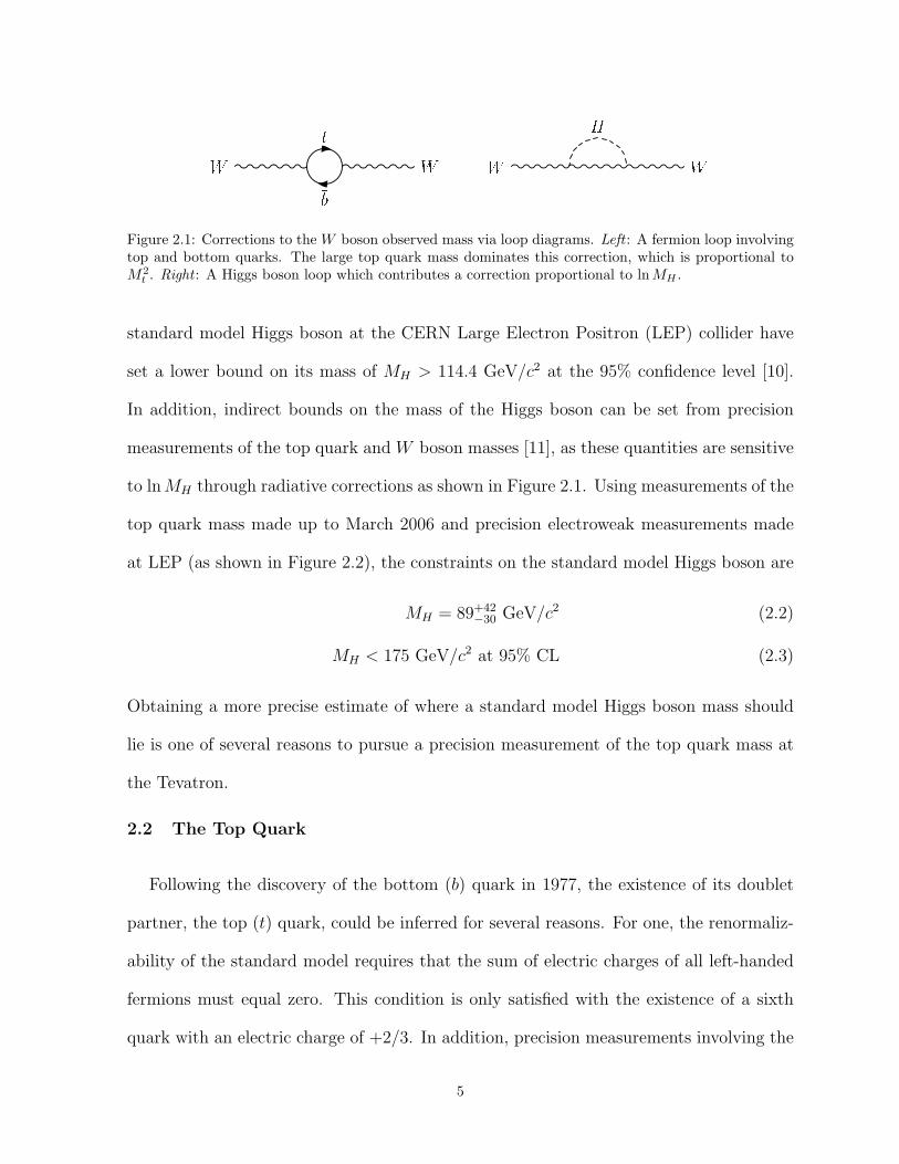
Figure 2.1: Corrections to the W boson observed mass via loop diagrams. Left : A fermion loop involvingtop and bottom quarks. The large top quark mass dominates this correction, which is proportional toM2
t . Right : A Higgs boson loop which contributes a correction proportional to lnMH .
standard model Higgs boson at the CERN Large Electron Positron (LEP) collider have
set a lower bound on its mass of MH > 114.4 GeV/c2 at the 95% confidence level [10].
In addition, indirect bounds on the mass of the Higgs boson can be set from precision
measurements of the top quark and W boson masses [11], as these quantities are sensitive
to ln MH through radiative corrections as shown in Figure 2.1. Using measurements of the
top quark mass made up to March 2006 and precision electroweak measurements made
at LEP (as shown in Figure 2.2), the constraints on the standard model Higgs boson are
MH = 89+42−30 GeV/c2 (2.2)
MH < 175 GeV/c2 at 95% CL (2.3)
Obtaining a more precise estimate of where a standard model Higgs boson mass should
lie is one of several reasons to pursue a precision measurement of the top quark mass at
the Tevatron.
2.2 The Top Quark
Following the discovery of the bottom (b) quark in 1977, the existence of its doublet
partner, the top (t) quark, could be inferred for several reasons. For one, the renormaliz-
ability of the standard model requires that the sum of electric charges of all left-handed
fermions must equal zero. This condition is only satisfied with the existence of a sixth
quark with an electric charge of +2/3. In addition, precision measurements involving the
5

80.3
80.4
80.5
150 175 200
mH [GeV]114 300 1000
mt [GeV]
mW
[G
eV]
68% CL
!"
LEP1 and SLDLEP2 and Tevatron (prel.)
0
1
2
3
4
5
6
10030 300mH [GeV]
!"2
Excluded
!#had =!#(5)
0.02758±0.000350.02749±0.00012incl. low Q2 data
Theory uncertainty
Figure 2.2: Left : Constraints on the standard model Higgs boson mass as a function of top quark massand W boson mass as of March 2006. The red curve shows the 68% CL constraint obtained from studiesat the Z pole made at SLD and LEP. The dashed blue curve shows the 68% CL constraint obtained fromdirect measurements of MW and Mt made at LEP and the Tevatron. Right : The ∆χ2 (black curve) to aglobal fit of standard model parameters to a standard model Higgs boson mass. The yellow band showsthe region excluded by direct searches at LEP. Courtesy of the LEP Electroweak Working Group [11].
isospin of the b-quark can be made at e+e− colliders which can be used to exclude the
possibility of the b quark being a member of a singlet [12]. The discovery of the top quark
was accomplished in 1995 at the CDF and DØ experiments[13, 14]. By the end of the
1992-1996 collider run (Run I), combined measurements from both experiments’ datasets
of ∼100 pb−1 provided a measurement of the top quark mass of Mt = 178± 4.3 GeV/c2.
2.2.1 Top Quark Production
In pp collisions, top quarks are predominantly produced in pair form via the strong
force. While single top quark production via the electroweak force is predicted in the
standard model, it has not been observed with statistical significance. At the current
Tevatron center-of-mass energy of√
s = 1.96 TeV, top-antitop pair (tt) production occurs
via the channel qq → tt approximately 85% of the time while occurring via the channel
6

Figure 2.3: Top: Leading-order production diagram for qq → tt. Bottom: Leading-order productiondiagrams for gg → tt.
gg → tt the remaining 15% of the time [15]. The leading order diagrams for these
production channels are shown in Figure 2.3.
The theoretical prediction of the tt production cross-section at Next-to-Leading Order
(NLO) is σNLOtt = 6.7+0.7
−0.9 pb for Mt = 175 GeV/c2 [15]. Figure 2.4 shows the NLO
calculation of σtt for pp collisions at√
s = 1.96 TeV as a function Mt. A combination
of current measurements of σtt made at CDF during the current collider run, Run II
(√
s=1.96 TeV) [16] are also shown, and is in good agreement with the predicted value.
2.2.2 Top Quark Decay
Nearly 100% of top quarks are expected to decay via the channel t → Wb. Other decay
channels are permitted in the standard model, but are heavily suppressed by factors of
|Vts|2/|Vtb|2 ≈ 10−3 and |Vtd|2/|Vtb|2 ≈ 5 × 10⁻⁴, where Vij is the Cabibbo-Kobayashi-
Maskawa (CKM) weak–mixing matrix [17]. For the purposes of this analysis, we will
assume that top quark decay occurs exclusively via the channel t → Wb. The large mass
of the top quark results in a very rapid decay with a mean lifetime of τt ∼ 10−24 s. As this
7

)2Top Quark Mass (GeV/c160 162 164 166 168 170 172 174 176 178 180
) (pb
)t t
! p(p
"
0
2
4
6
8
10
12
Cacciari et al. JHEP 0404:068 (2004)
uncertainty±Cacciari et al.
-1CDF II Preliminary 760 pb
Figure 2.4: NLO calculations of σtt [15] for pp collisions at√
s = 1.96 TeV as a function of Mt. Alsoshown are experimental measurements of σtt made at CDF using Run II [16] data.
is shorter than the timescale required for quarks to form bound states (or “hadronize”),
the top quark essentially decays as a “free” quark. The b-quark resulting from the decay
will then proceed to hadronize and manifest itself in the detector as a jet, or a collimated
stream of hadrons (jets are described further in Chapter 4). The W boson will decay
rapidly into either a pair of quarks or a charged lepton and a neutrino. Thus, for the case
of a tt pair decay, we have six particles in the final state: two b-quarks and two decay
products from each of the W bosons.
It is the decay mode of the W bosons that defines the decay channels of the tt system
used in its experimental study. These decay channels are classified as:
• The all-hadronic channel, where both W bosons decay to quarks, resulting in a final
state having an experimental signature of six jets. This decay mode carries the
largest branching ratio, of 46%, but suffers from the largest amount of irreducible
background due to its high jet count.
8

• The lepton+jets channel, where one W decays to a lepton and the other to quarks,
resulting in an experimental signature of a high momentum lepton, four jets, and
missing transverse energy3 associated with the neutrino. Due to the difficulty of
identifying τ leptons at a hadron collider, only leptonic states with an electron or
muon in the final state are considered. While the multi-jet background is still large
in this channel, it is far less than in the all-hadronic channel. This channel carries a
branching ratio of 30%.
• The dilepton channel, where both W bosons decay to leptons, resulting in an ex-
perimental signature of two high momentum leptons, two jets, and large missing
transverse energy associated with two neutrinos. As with the lepton+jets channel,
only leptonic states with an electron or muon on the final state are considered. A di-
agram showing this decay channel is in Figure 2.5. This channel carries a branching
ratio of 5%. The analysis described in this dissertation is performed in the dilepton
channel.
The remaining 20% of tt decays involve the production of a τ lepton that does not
decay to an e or µ. While measurements in this so-called “τ + X” channel are possible,
they does not afford nearly the same precision that any of the other three channels do.
2.3 Top Quark Mass in the Dilepton Channel
Traditionally, the lepton+jets channel has offered the most precise measurements of the
top quark mass due to its higher statistics than the dilepton channel and lower background
than the all-hadronic channel. However, the dilepton channel, while offering the least
amount of statistics, has some unique advantages. Since it has the least amount of jets,
the dilepton channel, in principle, offers the least reliance on the jet energy scale (the
3Assuming the transverse energy of the initial system is zero, an imbalance in final state transverse energy, or “missingtransverse energy” ( 6ET ) can be attributed to undetected objects, such as neutrinos. 6ET is described further in Chapter 4.
9

Figure 2.5: Decay of tt in the dilepton channel.
estimation of underlying parton energy from measured jet energy– described further in
Chapter 4). The jet energy scale is the single largest source of systematic uncertainty
in most top mass measurements. The lower number of jets also results in fewer possible
jet-parton combinations in each event. In addition, the dilepton channel has the highest
sample purity without the usage of explicit b-jet identification.4
The difficulty in measuring the top quark mass in the dilepton channel results arises
from the presence of two neutrinos in each event. As neutrinos cannot be directly detected
in our detector, their presence must be inferred from 6ET in an event. As there is only one
6ET measurement per event, the amount of energy imparted from each individual neutrino
can never be known in dilepton events. Therefore, the kinematic final state of the tt
cannot be fully reconstructed using measured quantities in dilepton events.
Despite the lower statistical precision of top quark mass measurements in the dilepton
channel, these measurements are still able to provide significant contributions to the
4B-jet identification methods such as secondary vertex tagging (the measurement of displaced secondary vertices inan event resulting from the decay of a b-jet) greatly reduce the amount of background in all tt channels at the cost ofapproximately 50% of the signal statistics. Such methods are used in nearly all precision measurements of the top quarkmass in the lepton+jets and all hadronic channels.
10

overall precision of our knowledge of the top quark mass. At the time of this writing, the
most recent combination of measurements of the top quark mass utilizes measurements
made with Run I data and up to 750 pb−1 of Run II data from both CDF and DØ [18].
This average and the individual measurements contributing to it are shown in Figure 2.6.
The single most precise measurement in the dilepton channel used for this combination,
a prior iteration of the analysis described in this dissertation, provides a weight of 11%.
A striking feature of Figure 2.6 is the relatively low value that precision measurements
of the top quark mass in the dilepton channel have relative to the most precise measure-
ments in the lepton+jets channel. While these deviations are certainly not inconsistent
with statistical fluctuations, a measurement of the mass of the top quark, assuming the
standard model, should yield the same value in all decay channels. A significant deviation
between decay channels could indicate the presence of non-standard model contributions
in one or more of the decay channels.
11

Mtop [GeV/c2]
Mass of the Top Quark (*Preliminary)Measurement Mtop [GeV/c2]
CDF-I di-l 167.4 ± 11.4
D!-I di-l 168.4 ± 12.8
CDF-II di-l* 164.5 ± 5.5
D!-II di-l* 176.6 ± 11.8
CDF-I l+j 176.1 ± 7.3
D!-I l+j 180.1 ± 5.3
CDF-II l+j* 173.4 ± 2.8
D!-II l+j* 170.6 ± 4.6
CDF-I all-j 186.0 ± 11.5
"2 / dof = 8.1 / 8
Tevatron Run-I/II* 172.5 ± 2.3
150 170 190
Figure 2.6: World average of the top quark mass along with the individual measurements used to calculateit as of March 2006 [18].
12

CHAPTER 3
Experimental Apparatus
The large mass of the top quark makes it necessary to rely on high-energy collisions to
produce them. At the time of this writing, the Tevatron synchrotron at the Fermi National
Accelerator Laboratory (Fermilab) in Batavia, Illinois, is the only facility with sufficient
energy for direct top quark production. Once produced, a device capable of observing the
resulting events is necessary. The CDF II detector is one of the two detectors built on
the Tevatron capable of performing this task. In this chapter, both the collider and the
detector are described.
3.1 The Collider
The collider complex at Fermilab consists of a chain of eight accelerators that are
necessary to take protons and not only accelerate them to a high energy, but also produce
antiprotons, accelerate them to the same energy, and collide them with protons at a
center-of-mass energy of√
s = 1.96 TeV. A schematic view of the Fermilab accelerator
complex is shown in Figure 3.1.
3.1.1 The Proton Source and Pre-Acceleration
The protons that are used in collisions and to produce antiprotons all begin in a small
bottle of hydrogen gas. Hydrogen atoms drawn from this bottle are ionized to form H−
13

_
F0
A0
E0 C0
_
B0
D0
NS
W
E
p
p
p
p
MAIN INJECTOR
(980 GeV)
(980 GeV)
(150 GeV)
Figure 3.1: A schematic view of the Fermilab accelerator complex. Figure courtesy of Fermilab Acceler-ator Division.
ions. The H− ions are accelerated from rest to an energy of 750 keV by a Cockroft-Walton
device– an electrostatic generator that applies an electric field to the ions.
The H− ions are then injected into the Linac, a linear RF accelerator, which further
accelerates them to an energy of 400 MeV. At this point, the electrons are removed from
the H− ions, leaving behind bare protons.
The protons then enter the Booster, a synchrotron with a circumference of 474 m.
The Booster utilizes magnets to bend the protons along a circular path while RF cavities
accelerate them to an energy of 8 GeV.
At this point, the protons enter the Main Injector, a synchrotron 3 km in circumference.
14

The Main Injector can accelerate the protons either to 150 GeV for injection into the
Tevatron, or to 120 GeV for usage in antiproton production. The Main Injector can also
stack antiprotons produced in the antiproton source and accelerate them to 150 GeV prior
to usage in the Tevatron.
3.1.2 The Antiproton Source
One of the most technically daunting tasks in the collider operations at Fermilab
is the production and storage of antiprotons. Because of its difficulty, the production
of antiprotons remains the limiting factor in the luminosity of colliding beams at the
Tevatron. The antiproton source at Fermilab consists of a target for production and three
accelerators used to cool and store: the Debuncher, the Accumulator and the Recycler.
Antiprotons are produced by striking 120 GeV protons from the Main Injector upon
a nickel target. These collisions yield a shower of particles from which antiprotons are
separated using magnetic spectroscopy.1 Approximately 100,000 protons are needed to
successfully produce and store one antiproton. The resulting antiprotons have an average
energy of 8 GeV.
The antiprotons produced at the target are then sent to the Debuncher, a triangular
synchrotron with a mean radius of 90 m. The beam of antiprotons sent into the Debuncher
has a large spread of momenta. The Debuncher is tasked with reducing this spread in
momenta, forming a continuous beam.
The antiprotons are sent to the Accumulator, another triangular synchrotron that
shares a tunnel with the Debuncher. Here, the antiprotons are stored, or “stacked”, as
more are produced. In addition, a process known as stochastic cooling is used to further
reduce the spread in momenta of the antiprotons. When a sufficient number of antiprotons
1The particles are subject to a magnetic field causing particles of different mass and charge to take paths of differentradii. This allows antiprotons to be separated out.
15
for colliding beam operations have been stacked at the Accumulator, they can then be
sent to the Main Injector for further acceleration.
The Recycler
The Recycler is a 3 km synchrotron housed in the same tunnel as the Main Injector.
It utilizes permanent magnets, making it the largest particle accelerator ever built that
solely uses permanent magnets. The original design of the Recycler called for it to store
antiprotons that were unused in a colliding physics run in the Tevatron and use them in
a future colliding run. In practice, this mode of operation proved difficult to implement
practically and efficiently. However, since 2004, the Recycler has been used to store
additional antiprotons prior to a colliding physics run. Antiprotons are now stored in
both the Accumulator and Recycler for nearly all colliding beam runs, greatly increasing
the amount of available antiprotons for collisions in the Tevatron.
Electron Cooling
Electron cooling is a technique which uses a beam of electrons run alongside a beam of
antiprotons to reduce the longitudinal momentum of the antiprotons. While the method
was first proposed in 1966 and has been utilized for low-energy beams, its implementation
at Fermilab in 2005 is the first successful application of electron cooling to a relativistic
beam. The electron cooling system in use utilizes a 4.3 MeV beam of electrons that is
run alongside a 20 m length of the Recycler. This system has been in operation since late
2005 and is expected to help increase luminosities for the colliding beams by up to 100%
from pre-electron cooling peak luminosity.
3.1.3 The Tevatron
The final stage of acceleration occurs in the Tevatron. A synchrotron with a circum-
ference of 6.3 km, the Tevatron utilizes superconducting magnets with field strengths up
16

to 4.2 T. Both the protons and antiprotons are injected into the Tevatron from the Main
Injector in bunches, at an energy of 150 GeV. For colliding physics runs, 36 bunches each
of protons and antiprotons are injected in the Tevatron. The bunches are spaced such
that they cross every 396 ns. Once in place, the Tevatron accelerates these bunches to
an energy of 980 GeV. The Tevatron is divided into 6 sectors lettered “A” through “F”
and each sector is further subdivided into 5 segments numbered 0-4 (the locations of A0
through F0 are shown in Figure 3.1). Each 0 segment contains a long straight section of
the accelerator. Both the B0 segment (where the CDF detector sits) and the D0 segment
(where the aptly named DØ detector sits) have quadrupole magnets that focus the beams
and steer the proton and antiproton bunches into one another for collisions. The focusing
reduces the beam spot size and thus increases the instantaneous luminosity of the beam.
The instantaneous luminosity is given by
L =NBNpNpf
2πσ2pσ
2p
, (3.1)
where NB is the number of bunches present in the accelerator, Np and Np are the number
of protons and antiprotons per bunch, f is the bunch revolution frequency, and σp and
σp are the effective widths of the proton and antiproton bunches. Integrated luminosity,∫Ldt, when combined with the cross-section for pp collisions, gives a measure of the
number of collisions in a given period of time. Figure 3.2 shows the total integrated
luminosity at CDF as of February 2006. The analysis presented in this document was
performed using an integrated luminosity of∫Ldt = 1.0 fb−1. For comparison, the total
integrated luminosity in Run I was∫Ldt = 125 pb−1.
3.2 The CDF Detector
The CDF detector is an azimuthally and forward-backward symmetric detector de-
signed to study pp collisions at the Tevatron. A schematic overview of the CDF detector
17

Store Number
To
tal
Lu
min
osi
ty (
pb
-1)
0
200
400
600
800
1000
1200
1400
1600
1000 1500 2000 2500 3000 3500 4000 4500
1 4 7 10 1 4 7 10 1 4 7 1 4 7 102002 2003 2004 2005 2006Year
Month
DeliveredTo tape
Figure 3.2: The total integrated luminosity at CDF as of February 2006. The red curve shows the totalintegrated luminosity delivered to CDF while the blue curve shows the total integrated luminosity writtento tape at CDF.
is shown in Figure 3.3.
The CDF coordinate system is right-handed, with the z-axis pointing along a tangent
to the Tevatron ring along the proton direction. The remaining rectangular coordinates
x and y are defined pointing outward and upward from the Tevatron ring respectively.
Often, it is more convenient to work in polar coordinates (which are facilitated by the
symmetry of the CDF detector in the xy-plane), where r ≡√
x2 + y2 + z2 and φ ≡
tan−1(y/x). The canonical third variable in the polar coordinate system is θ ≡ cos−1(z/r).
However, θ is not invariant under longitudinal boosts. Since the constituent particles of
the proton and the antiproton will not have an initial energy of 980 GeV, the production
18

Figure 3.3: A cross-sectional view of the CDF detector [19].
of particles as a function of angle will depend on the initial velocities of the constituent
particles. The rapidity, defined as:
ζ ≡ 1
2ln
E + pz
E − pz
(3.2)
is invariant under boosts along the z-axis. For the massless case (p � m), the rapidity
can be approximated as the pseudo-rapidity, defined as:
η ≡ − ln tanθ
2. (3.3)
This coordinate is invariant under Lorentz transformation and is used as the third coor-
dinate in the CDF coordinate system.
The basic structure of the CDF detector can be subdivided from the inside (starting
19

at the beampipe) out into: the tracking system (responsible for measuring momenta of
charged particles), the calorimeters (responsible for measuring the energy of interacting
particles), and the muon system (responsible for identifying muons).
3.2.1 The Tracking System
The CDF tracking system consists of a silicon microstrip tracker and an open-cell drift
chamber. The silicon tracker consists of three subdetectors, listed in order of distance from
the beampipe: Layer 00 (L00), the Silicon VerteX detector (SVX), and the Intermediate
Silicon Layers (ISL). The drift chamber, known as the Central Outer Tracker (COT),
surrounds the silicon tracking system.
The entire CDF tracking system is immersed in a 1.4 T magnetic field that is generated
by a superconducting solenoid magnet. The solenoid has a radius of 1.5 m, is 5 m in length
and has a stored energy of 30 MJ when at full field strength. The magnetic field produced
by the solenoid is uniform along the direction of the z-axis. Charged particles within the
magnetic field follow helical trajectories. The radius of curvature and the orientation of
the helix can be used to determin the momentum and charge of a charged particle. A
schematic overview of the CDF tracking system is shown in Figure 3.4.
Silicon Detector
The silicon detector, which provides high-resolution position measurements of charged
particles close to the interaction region, consists of three subdetectors. The main subde-
tector is the SVXII [20] detector, a five layer, double-sided silicon detector that covers
the radial region between 2.5 cm and 10.6 cm. The SVXII detector is composed of three
cylindrical barrels, each 16 cm long in the z-direction (see Figure 3.5). Each barrel is
divided into 12 azimuthal wedges of 30◦ each. Each of the five layers in a wedge is fur-
ther divided into electrically independent modules called ladders. There are a total of
20

0
.5
1.0
1.5
2.0
0 .5 1.0 1.5 2.0 2.5SVX Intermediate Silicon Layers
m
3.0
End WallHad. Cal.
30
3 00 = 1.0
= 2.0
= 3.0
n
n
n
m
End
Plug
Had
ron
Calor
imet
er
End
Plug
EM
Cal.
Central Outer Tracker
1.4 Tesla Solenoid
Figure 3.4: A schematic overview of the CDF tracking system. The region of the detector with |η| < 1.0is referred to as the “central” region.
360 ladders in the SVXII detector. The double-sided silicon microstrips of the SVXII
detector are arranged so that one side is aligned with the z-axis (known as “axial” strips)
and the other side is either at an angle of 90◦ or 1.2◦ with respect to the axial layer.
These arrangements make it possible to make three-dimensional position measurements
by combining the (r − φ) and (r − z) measurements.
The innermost subdetector of the silicon detector, Layer 00 (L00) [21], is a single-
sided layer of silicon wafers mounted directly on the beampipe at a radius of 1.6 cm and
provides measurements closest to the interaction point. The outermost subdetector, the
Intermediate Silicon Layers (ISL) [22], is comprised of one or two additional layers of
21

Chapter 2: Detector 78
Silicon Vertex Detector II (SVXII)
The Silicon Vertex Detector II ([24]) is the primary detector of the silicon sub-
systems. It is comprised of 5 layers of double sided silicon strip detectors. In all five
layers, there is an R ! ! strip, in three layers there are 90! strips, and the other two
have 1.25! strips. The R ! ! strips are situated lengthwise on the p-n junction of
the detector, and both the 90! and 1.25! strips are located on the n-side. The strips
are situated in three cylindrical barrels, each 30 cm long. There are 360 “ladders”
(four sensors connected by wire bonds) in 12 x 30! !-slices. The radii of the layers
are between 2.5 cm and 10.6 cm. Figure 2.13 shows the barrel structure of the SVXII
detector.
Table 2.2 compares the technical specifications of the Run I and Run II detectors.
Figure 2.13: SVXII barrel structure.
Figure 3.5: The SVX barrel structure [19].
double-sided silicon, depending on the polar angle, at radii from 20 cm to 28 cm. The
ISL serves to extend silicon tracking coverage up to |η| < 2. Combined, the CDF silicon
detector has a total of 722,432 channels.
COT
The Central Outer Tracker (COT) [23], a large open-cell drift chamber, is positioned
outside the silicon detector from radii of 0.43 m to 1.32 m. The COT contains 8 “su-
perlayers” each containing 12 wire layers for a total of 96 layers. Four of the superlayers
provide R− φ measurements (axial superlayers) while the other four provide 2◦ measure-
ments (stereo superlayers). The drift chambers are filled with a 1:1 mixture of argon and
ethane. This mixture provides for a maximum drift time of 177 ns with a drift velocity
of 100 µm/ns, which prevents pileup of events in the drift chamber from previous events.
The resulting transverse momentum resolution of the COT is σpT/pT ≈ 0.15%× pT .
22

System Coverage in η Thickness Energy Resolution
CEM |η| < 1.1 18X0, 1λ 13.5%/√
ET ⊕ 2%
PEM 1.1 < |η| < 3.6 21X0, 1λ 16%/√
E ⊕ 1%
CHA |η| < 0.9 4.5λ 50%/√
ET ⊕ 2%
WHA 0.7 < |η| < 1.2 4.5λ 75%/√
E ⊕ 4%
PHA 1.2 < |η| < 3.6 7λ 80%/√
E ⊕ 5%
Table 3.1: Properties of the CDF II calorimeter systems. The energy resolutions for the electromagneticcalorimeters are for electrons and photons; the resolutions for the hadronic calorimeters are for isolatedpions.
In combination the Silicon and COT detectors provide excellent tracking up to |η| ≤ 1.1
with decreasing coverage to |η| ≤ 2.0.
3.2.2 Calorimeters
The CDF calorimetry system sits outside the solenoid and is responsible for measuring
particle energies. The calorimeters comprising it sample electromagnetic and hadronic
showers produced as particles traversing them interact with dense material. The system
covers a full 2π in azimuth and is subdivided into a “central” region (|η| < 1.1) and a
“plug” region (1.1 < |η| < 3.6). Each calorimeter is segmented into “towers”, containing
alternating layers of scintillator and inert material. Each calorimeter system described
below consists of an electromagnetic component and a hadronic component. The elec-
tromagnetic component measures the energy of electrons and photons by sampling elec-
tromagnetic showers caused by bremsstrahlung of the electron or e+e− pair production
of the photon. The hadronic component measures the energy of hadrons and jets by
sampling electromagnetic showers due to neutral meson production and their subsequent
electromagnetic decay and hadronic showers due to strong interactions of hadrons with
heavy atomic nuclei. A summary of the CDF calorimeter systems is shown in Table 3.1
23

The Central Calorimeter
In the central region of |η| < 1.1, the calorimeter towers subtend 15◦ in φ and 0.1 in η.
The central electromagnetic calorimeter (CEM) [24] constitutes the front of the wedges
in the central region. The CEM consists of alternating layers of lead and scintillator,
amounting to 18 radiation lengths2 of material. Embedded in the CEM is the shower
maximum detector (CES). The CES provides position measurements of the electromag-
netic showers at a depth of 5 radiation lengths and is used in electron identification.
Behind the CEM is the central hadronic calorimeter (CHA) [25], which provides energy
measurements of hadronic jets. The CHA consists of 4.7 interaction lengths3 of alternating
steel and scintillator. The CHA covers the region up to |η| < 0.9.
The End-Wall and Plug Calorimeter
Since the CHA covers only the region up to |η| < 0.9, the end-wall hadronic calorimeter
(WHA) was constructed to cover the region from 0.7 < |η| < 1.2. Its construction
is otherwise very similar to the CHA. The plug electromagnetic calorimeter (PEM) [26]
consists of alternating lead absorber and scintillating tile readout with wavelength shifting
fibers; the total thickness is 23.2 radiation lengths of material. A plug shower maximum
detector (PES) [27] provides position measurement of electron and photon showers. The
plug hadronic calorimeter (PHA) has alternating layers of iron and scintillating tile for a
total of 6.8 interaction lengths.
3.2.3 The Muon Detector
As muons are 200 times more massive than electrons, they lose considerably less energy
due to bremsstrahlung in the calorimeter and thus are effectively not detectable by the
2The radiation length, X0, is defined as the distance over which a high-energy electron loses all but 1/e of its energy bybremsstrahlung.
3The interaction length, λ, is defined as the mean free path of a particle before undergoing an inelastic nuclear interaction.
24

- CMX - CMP - CMU
φ
η
0 1-1
Figure 2.11. η and φ coverage of the CDF II muon system.
30
Figure 3.6: Coverage of the CDF muon systems.
calorimeter. Thus, the muon detectors sit on the very outside of the CDF detector, and
are separated from the calorimeter by a layer of steel shielding. This layer of shielding
serves to absorb charged pions which can traverse the whole of the calorimeter and could
incorrectly be interpreted as muons. Unlike the tracking and calorimetry systems, the
muon system is incomplete in φ, due to space constraints. Its coverage is shown in
Figure 3.6.
The muon detection system consists of three sandwiched drift tube layers, each utilizing
single wire drift cells four layers deep. Directly behind the central hadronic calorimeter
and the layer of steel shielding is the central muon detector (CMU) [28] which can detect
muons with pT > 1.4 GeV/c in the region of |η| < 0.6. Additional muon coverage in this
region is provided by the central muon upgrade (CMP) which is separated from the CMU
25

by 60 cm of steel. The CMP detects muons with pT > 2.0 GeV/c. The central muon
extension (CMX) provides further coverage in the region of 0.6 < |η| < 1.0.
3.2.4 Trigger System
Of the over 2 million pp collisions that occur every second during operation of the
Tevatron collider, the vast majority are not interesting in the study of high energy physics.
CDF employs a three-level trigger system to select events involving physically relevant
phenomena and record them, while rejecting uninteresting events. Due to the physical
limitations involved in physical storage and the rate at which data can be stored, the
trigger system must reduce the data acquisition rate from the approximately 2 MHz
collision rate to approximately 75 Hz. An overview of the CDF Trigger system is presented
in Figure 3.7.
Level 1 Trigger
The level 1 trigger utilizes custom designed hardware to make decisions based on
simple physics quantities within events. Raw information from the detector from every
beam crossing is stored in a pipeline capable of buffering data from 42 beam crossings.
Processing of this data takes place in one of three streams. One analyzes calorimeter
information to identify objects that may further be reconstructed into electrons, photons
or jets. Another stream searches for track segments in the muon detector, or “stubs”,
which may be used in conjunction with tracks in the tracking system to reconstruct muons.
The third stream utilizes tracking data to identify tracks that can be linked to objects in
the calorimeter or muon detector. The level one trigger decision takes place 5.5 µs after
a collision and reduces the event rate to approximately 50 kHz.
26

!"#"$%&
'()**"(
!"#"$%+
'()**"(
,"-"./)01%23./0(45.."6/%(3/" 7%89%:;
<%=
>3??
@/0(3*"
!?%A%+B9C%D:;E%&C
!"#$%%&'(
!)#$%%&'(
+=%.$0.D
.F.$"?%G""6
HI'IJ'K,
!+%?/0(3*"
6)6"$)1"4
H5L%MN22"(?%BI#"1/%ON)$G"(
!"#"$%P
@F?/"Q
=%"#"1/?
!&%MN22"(?4
5?F1.R(010N?%&!?/3*"%6)6"$)1"
!+S!&%("-"./)01%23./0(4 &9TCCC
PUV%1? .$0.D%.F.$"WXJ(0??)1*%(3/"
&Y9P%>:; ?F1.R(010N?%6)6"$)1"!3/"1.F5.."6/%(3/" 7%9C%D:;
99==%1?%A%=&%Z%+P&%1?
!3/"1.F5.."6/%(3/" PCC%:;
&Y9P%>:;
Figure 4.1: CDF Data Acquisition system
37
Figure 3.7: The CDF Trigger and Data Acquisition System.
Level 2 Trigger
The level 2 trigger utilizes programmable processors to perform limited event recon-
struction on events accepted by the level 1 trigger. These events are then stored in one
of four asynchronous buffers and a decision is made as to whether the events pass one
of the pre-defined level 2 trigger criteria. The decision time for the level 2 trigger is ap-
proximately 25 µs. The level 2 trigger further reduces the event rate to approximately
300 Hz.
Level 3 Trigger
The level 3 trigger consists of two components: an “event builder” that uses custom
hardware to assemble data from all subdetectors of CDF into a reconstructed event, and
27

a large processing farm consisting of commodity computing hardware. Each processor
in the processing farm can then make a decision as to whether an event reconstructed
by the event builder satisfies pre-defined level 3 trigger criteria. The level 3 trigger then
separates events into streams based on the physics objects that resulted in their trigger
and commits them to permanent storage. The level 3 trigger reduces the event rate to
approximately 75 Hz.
28

CHAPTER 4
Data Sample and Event Selection
We select tt → b`ν`b`′ν`′ decays with a high-pT lepton trigger and the requirement that
candidates have (i) two leptons each with pT > 20 GeV/c, (ii) significant missing energy
transverse to the beam direction (6ET ), and (iii) two jets each with ET > 15 GeV. Missing
transverse energy is calculated as
6ET = −∑
i
EiT~ni, (4.1)
where EiT are the magnitudes of transverse energy contained in each calorimeter tower i,
and ~ni is the unit vector from the interaction vertex to the tower in the transverse (x, y)
plane. 6ET is corrected for the presence of isolated high-pT muons by subtracting the
momentum lost by the muons in the calorimeter and adding the muon pT to the vector
sum.
The selection was designed for a cross-section measurement and is described as “DIL”
in [29]. A description of the trigger requirements and selection used to obtain this dataset
follows.
4.1 Trigger Requirements
The trigger requires at least one high-pT lepton. For central electron candidates, the
first two trigger levels require an electromagnetic calorimeter cluster with a confirming
29
track in the COT and without a large hadronic energy deposit. The third level trigger
requires an electron candidate with ET ≥ 18 GeV. Events with electron candidates in
the plug (|η| > 1.2) are required to have electron ET > 20 GeV and 6ET > 15 GeV. For
muon candidates, the first two trigger levels require hits in the muon chambers and a
confirming COT track. The third level trigger requires a muon stub with a matching
track of pT ≥ 18 GeV/c.
4.2 Event Selection
4.2.1 Leptons
After offline event reconstruction, tighter cuts are placed on the leptons that pass the
basic trigger requirements.
Electron candidates are required to have an electromagnetic calorimeter cluster with
ET > 20 GeV and muon candidates to have a track with pT > 20 GeV/c. At least one of
the leptons is required to be isolated in the calorimeter, where the lepton contains at least
90% of the total ET within a cone ∆R ≡√
(∆η)2 + (∆φ)2 = 0.4. In addition, electron
candidates are required to have a well-measured track pointing at an energy deposition
in the calorimeter. For electron candidates with |η| >1.2, this track association uses a
calorimeter-seeded silicon tracking algorithm [30].
Muon candidates are required to have a well-measured track linked to hits in the
muon chambers and energy deposition in the calorimeter consistent with that expected
for muons. If the event contains two muons, only one is required to have hits in muon
chambers used in the trigger decision. The other muon may have hits in chambers not
used for the trigger decision if there is a matching COT track, or no hits in muon chambers
if the COT track points in regions where there is no muon chamber coverage.
30

4.2.2 Jets
Quarks and gluons formed in collisions or from decays of other particles will either im-
mediately decay (in the case of the top quark), or fragment and combine with other quarks
and gluons to form color-neutral particles called hadrons1, a process called hadronization.
This process usually results in a stream of energetic hadrons with momenta distributed
in a cone around the direction the original quark or gluon was traveling. This object is
referred to as a hadronic jet, or simply, a jet. While hadronization makes direct measure-
ment of a quark or gluon’s momentum impossible, the energy and direction of a jet can
be used to infer the momentum of the underlying quark or gluon.
Jets are identified using a process called clustering; the clustering algorithm used at
CDF is called jetclu [31]. Jet clustering is done by first identifying an energetic tower
with ET > 1 GeV, called a “seed tower.” The energy of all the towers in a cone of
∆R = 0.4 around the seed tower is then calculated. A new centroid of the tower is then
calculated as:
η =
∑i E
iT ηi∑
i EiT
, φ =
∑i E
iT φi∑
i EiT
, (4.2)
where the sum is performed over all towers in the cluster. A cone of ∆R = 0.4 is then
drawn around the new cluster centroid, and the above process is repeated until the cluster
remains unchanged. After the clustering process is completed, the “raw” jet energy can
be calculated.
The jets resulting from the b-quarks in the top decay carry the most kinematic infor-
mation about the mass of the parent top quark of any of its decay products. However,
since jets are measured with poor energy resolution relative to leptons, they also are the
largest source of uncertainty in the measurement of the top mass.
1Hadrons are particles formed from the combination of a quark and anti-quark (called “mesons”) or three quarks orantiquarks (called “baryons”).
31

!-4 -3 -2 -1 0 1 2 3 4
-0.6
-0.55
-0.5
-0.45
-0.4
-0.35
-0.3
-0.25
-0.2
-0.15
-0.1
+ jets Samples. Cone 0.4 jets"
Data
Pythia
Herwig
+ jets Samples. Cone 0.4 jets"
Data
Pythia
Herwig
pje
tT
/p! T!
1
Figure 4.1: pjetT /pγ
T − 1 in γ+jets events as a function of η of the jets after relative corrections areapplied. Response is seen to be nearly flat for data as well as for events simulated with Pythia [33] orHerwig [34].
Jet Corrections
A series of corrections is made to raw jet energies to best approximate parton ener-
gies. These corrections are largely derived in dijet and minimum bias samples which are
independent of the underlying physics process and are described in detail in Ref. [32].
First, a dijet balancing procedure is used to correct for non-uniformities in the response
of the calorimeter as a function of η; these corrections are referred to as “relative correc-
tions.” Events with exactly two jets, one of which is in the central region, are chosen.
The knowledge that the ET of both jets should be equal is used to extract a correction
as a function of the jet pT and η. The relative correction ranges from +15% to -10%.
Applying this correction to both γ+jets data and simulated events from two different
event generators, we find that the calorimeter response is almost flat with respect to η as
seen in Figure 4.1.
A small, approximately 1%, correction is then applied for events containing multiple
32

pp collisions in the same accelerator bunch. This correction is needed to account for
energy from different collisions in the same bunch falling inside the jet cluster and thus
increasing the energy of the measured jet. In addition, a correction is made to subtract
energy associated with spectator partons in the underlying event.
Finally an absolute scale correction is needed to account for any non-linearity and
energy loss in the un-instrumented regions of each calorimeter. The response of the
calorimeter is measured using E/p of single tracks in the data. Studies of energy flow and
jet shapes in the data are also used in constraining the modeling of jet fragmentation.
This information is used to tune the simulation to model observations in the data, and
high statistics simulation samples are then used to extract the approximately 10-30%
absolute scale correction.
After the above corrections, the momentum components of each b quark are estimted
from the measured jet ET and angle assuming a b quark mass of 4.7 GeV/c2 [8]. Events
are then required to have at least two jets with |η| < 2.5 and ET > 15 GeV.
4.2.3 Final Selection Cuts
After lepton and jet identification, further requirements are made to reduce the ex-
pected level of background in the sample. Events are required to have missing transverse
energy of 6ET > 25 GeV. In events with 6ET < 50 GeV, the direction of the 6ET vector is
required to be separated by at least 20◦ in φ from any lepton or jet in the event. This
reduces the background from Drell-Yan production of τ pairs as well as the number of
events in which mismeasured jet or lepton energy contributes a large fraction of the 6ET .
To reduce the number of Z/γ∗ → ee, µµ events in which mismeasured jet energy
leads to significant amounts of measured missing tranverse energy, ee and µµ events with
dilepton invariant mass between 76 and 106 GeV/c2 are required to have their 6ET vector
33

point away from any energetic jets in the event. This is done by requiring these events to
have jet significance σjet > 8.0, where jet significance is defined as:
σjet ≡6ET√∑
k(6ET · EkT )
, (4.3)
where the sum is performed over all jets passing jet selection cuts defined in Section 4.2.2
that are in the same hemisphere as 6ET .
To further suppress background, events are required to have HT , defined as the scalar
sum of ET of all leptons and jets passing the above cuts and 6ET , greater than 200 GeV.
Events which are likely to be due to cosmic rays are removed by requiring a coincidence
of the muon arrival times to the calorimeter. Electrons resulting from photon conversion
to e+e− pairs are also removed. Conversions are identified by pairing the electron track to
a track of opposite sign and requiring that the two tracks are consistent with originating
from a common vertex and being parallel at that vertex. Events with three leptons are
removed as well as events in which the leptons have the same sign (no such events are
found in the data after all other selection cuts have been made).
4.3 Backgrounds
While the selection criteria above are designed to minimize the amount of background
in the sample, approximately 40% of the final dilepton top sample is expected to be
composed of background events.
The largest source of background in the sample is Drell-Yan (Z/γ∗) decaying to ee and
µµ final states with associated jets. Since there are no neutrinos in these events, in order
to pass the 6ET cut, they must have substantial 6ET resulting from mismeasurement of the
jet energies. Because of this, the contribution of this background is estimated using Z
events in data as well as Monte Carlo events.
34
The second largest source of background in the sample are events in which an object
is incorrectly identified as a lepton, or “fake” events. These events are mostly the result
of W → `ν+jets events where one jet gets reconstructed as a lepton. The contribution to
the final sample from these events is determined by applying a lepton fake rate to a data
sample of W → `ν+jets events. The lepton fake rate is determined using a large data
sample collected using a trigger on jets with ET > 50 GeV from which known sources of
real leptons are removed.
The remaining sources of background, including diboson (WW and WZ) production
with associated jets and Z/γ∗ → ττ events are smaller and have their contributions
estimated using Alpgen [35] Monte Carlo events of each process.
All remaining sources of background are assumed to have negligible contribution to
the sample.
4.4 Sample Composition
The accuracy of the background predictions for the DIL selection can be tested by
predicting the number of events expected in the sample with exactly one jet or no jets
passing the selection cuts. These events are expected to be nearly entirely background.
The predicted number of events can compared to the number seen in the data with zero
or one jets. As seen in Figure 4.2, the events in the data agree well with the prediction
for the background events.
Table 4.1 lists the number of expected background events of each type and the number
of tt signal events expected at various top quark masses [15] for the data sample used
in this measurement. The signal estimate includes tt events in which a W decays to a
τ when the τ decays to an e or a µ. Studies in Monte Carlo simulations show that 14%
of the accepted signal events have at least one W decaying to a τ . In the 1.0 fb−1 data
35

Jet Multiplicity0 1 2 3
Even
ts
0
20
40
60
80
100
120
140
160
180
200 = 6.7 pb)!tt (FakesWWWZ
""#ZZdata
+OSTH
Figure 4.2: The predicted jet multiplicity of events in the DIL selection with that observed in the dataoverlaid. The first three bins contain events that have not had the HT and opposite sign cut applied tothem while the final bin contains events passing all selection cuts outlined in this chapter.
sample used, 78 events satisfy all of the selection cuts described in this chapter.
The fraction of tt events that will pass our selection criteria will increase as a function
of the true top mass. This is due to the fact that a more massive top quark will have
more energetic decay products that are more likely to pass the kinematic selection cuts in
place. We calculate the overall acceptance of the selection criteria used by applying it to
tt events simulated with Herwig [34] at a range of top quark masses. The acceptance at
each mass, along with a second-order polynomial fit to these points is shown in Figure 4.3.
36

Source Eventstt (Mt = 165 GeV/c2, σ = 9.1pb) 63.4± 1.7tt (Mt = 175 GeV/c2, σ = 6.7pb) 50.2± 1.7tt (Mt = 185 GeV/c2, σ = 4.9pb) 38.9± 1.7Total Expected Background Rate 26.9± 4.8
WW 3.8± 1.0WZ 1.3± 0.2Z/γ∗ → ee, µµ 10.9± 4.4Z/γ∗ → ττ 2.2± 0.5Fakes 8.7± 1.5
Total Expected Rate (Mt = 165 GeV/c2) 90.3± 5.1Total Expected Rate (Mt = 175 GeV/c2) 77.1± 5.1Total Expected Rate (Mt = 185 GeV/c2) 65.8± 5.1Observed in Data (
∫Ldt = 1.0 fb−1) 78
Table 4.1: Expected numbers of signal and background events for a data sample of∫Ldt = 1.0 fb−1.
The signal cross section is obtained from [15]. The total expected background is the sum of the indentedbackground contributions.
(GeV)tM140 160 180 200 220
Acceptance
0.004
0.005
0.006
0.007
0.008
0.009
0.01
0.011
/ ndf 2! 19.55 / 16Prob 0.241p0 0.001817± -0.01483 p1 2.152e-05± 0.0001974 p2 6.236e-08± -3.727e-07
/ ndf 2! 19.55 / 16Prob 0.241p0 0.001817± -0.01483 p1 2.152e-05± 0.0001974 p2 6.236e-08± -3.727e-07
Figure 4.3: The Acceptance of the DIL selection criteria as a function of top quark mass. The sample ofsimulated event used is generated using the Herwig generator [34] and includes tt decays to all standardmodel decay channels with the theoretically predicted branching ratios. The parameterization shown isfor a fit to the function A = p0 + p1Mt + p2M
2t .
37

CHAPTER 5
Method Overview
The most commonly used approach to measure the top quark mass has been to use
template-based methods. These methods measure a reconstructed mass1 per event and
compare the distribution of reconstructed mass in the data to templates from a variety
of top quark masses. The calculation of a reconstructed mass requires making several
kinematic assumptions (e.g. the invariant masses of both intermediate-state W -bosons
being equal). The templates are parameterized using Monte Carlo event generators and
detector simulations. Template-based methods have been used to make all measurements
of the top quark mass in the dilepton channel from Run I data [36, 37]. Since these meth-
ods utilize fully simulated events to form templates, they take into account all detector
effects accounted for in the simulation. However, only a single number, a reconstructed
mass, enters into the final likelihood per event. In addition, all events, regardless of their
kinematic consistency with the tt process, have equal weight in the final likelihood.
A different class of methods, such as the one used in this analysis, utilizes our theo-
retical knowledge of the underlying physics processes to construct per-event likelihoods.
These methods, commonly known as “matrix-element methods,” are grounded in ideas
proposed before the discovery of the top quark [38, 39] and pioneered for usage in the
1This approach can be used using any kinematically reconstructible quantity, such as the event mass.
38

lepton+jets channel [40, 41, 42].
We construct per-event likelihoods by convolving the matrix element for tt decays and
detector resolution functions. Rather than making the kinematic assumptions made in
template-based methods, we instead integrate over unmeasured quantities. This allows for
maximal extraction of information from each event as the full phase-space of unmeasured
quantities is explored via integration. The final joint likelihood is a product of the per-
event likelihoods. This procedure weights events according to the relative amount of
information they carry. For computational tractability, a series of simplifying assumptions
must be made. These assumptions are accounted for by calibrating the final response of
the method using simulated events.
This chapter provides a brief overview of the method used. More detailed descriptions
of each part of the method are provided in chapters 7, 8, and 9.
5.1 Signal Likelihood
The probability density for tt decays is expressed as Ps(x|Mt), where Mt is the top
quark pole mass and x is a vector of measured quantities in the event (lepton momenta,
jet momenta and missing transverse energy). We calculate Ps(x|Mt) using the theoretical
description of the tt production and decay process expressed with respect to x,
Ps(x|Mt) =1
σ(Mt)
dσ(Mt)
dx, (5.1)
where dσdx
is the differential cross section evaluated with respect to event measurements
contained in x.
If the momenta of the initial-state and final-state partons were known exactly, the
evaluation of the differential cross section would reduce to the expression
dσ(Mt)
dx=
∫dΦ|Mtt(q1, q2,p; Mt)|2fPDF (q1)fPDF (q2), (5.2)
39

where M is the leading order matrix element for top pair production and decay, q1
and q2 are the initial state partons, p is a vector of final state particle momenta, fPDF
are the parton distribution functions2 [43], and dΦ is the phase space for the process
qq → tt → blνlbl′νl′ .
The matrix element depends on the momenta of the incoming partons (q1 and q2),
and of the outgoing two b-quarks (p1 and p2), two leptons (`1 and `2), and two neu-
trinos (ν1 and ν2). Observed quantities consist of jets (j1, . . . ji), measured leptons (L1
and L2), and two components of missing transverse energy. To express the differential
cross section with respect to these observed quantities x, transfer functions are intro-
duced to connect the quantities which correspond to external legs of the matrix element
(q1, q2, p1, p2, l1, l2, ν1, ν2) to the observed quantities (j1, . . . , ji, L1, L2). Quantities which
are well-measured by the detector, lepton momenta and jet angles, are described by delta
functions which directly reduce the number of unknown parton-level quantities. Inte-
grations are performed over quantities which are not directly measured, i.e. quark and
neutrino energies. While quark energies are not directly measured, they can be estimated
from the observed energies of the corresponding jets. The transfer function between
quark and jet energies parameterizes this relationship, and is expressed as W (Ep, Ej), the
probability of measuring jet energy Ej given parton energy Ep.
We make the following assumptions regarding the transfer between parton-level quan-
tities and the observables:
• Leptons are measured perfectly. We express the lepton transfer functions as a three-
dimensional δ-function,
δ3(`1 − L1) δ3(`2 − L2).
2The Parton Distribution Functions (PDFs), describe the probability that a parton, q, will carry a given fraction of themomentum of the system.
40

• Jet angles are measured perfectly, and jet energy can be described as a parametric
function of parton energy. We express the b-quark to jet transfer function as
δ(θj1 − θp1)δ(φj1 − φp1)W (Ep1 , Ej1)W (Ep2 , Ej2).
• Incoming partons are massless and have no transverse momentum.
• The two leading jets come from b-quarks.
• Masses of the final state leptons are zero, masses of the b-quarks are set to 4.7
GeV/c2.
These assumptions, while reasonable approximations, are not fully held in realistic events,
resulting in the measured statistical uncertainty being underestimated in these events.
The effect of these assumptions is considered in detail in Chapter 7. We can correct for this
effect by performing pseudo-experiments of simulated events as described in Chapter 9.
The probability density in x for qq → tt → b`−ν`b`′+ν ′` for a fixed Mt can be written
as
Ps(x|Mt) =1
σ(Mt)
∫dΦ
∑a,b
|Mtt(qi, pi; Mt)|2W (p, x)faPDF(q1)f
bPDF(q2). (5.3)
In this expression, the integral is over the phase space dΦ for qq → tt → blνlbl′νl′ , the
sum runs over the flavors a, b of the incoming partons, and faPDF are parton distribution
functions for flavor a. The transfer functions, W (p, x), link the measured quantities x to
the parton-level ones, p, and are described in detail in Chapter 6. Constraints such as
conservation of momentum which appear as delta functions and modify the integration
are here implicitly included in the phase-space integration and are discussed in detail in
Chapter 7. The term, 1/σ(Mt), in front of the integral ensures the normalization condition
41

for the probability,
∫dx Ps(x|Mt) = 1, (5.4)
where the integration is performed over all accepted x to account for mass-dependent
effects of the selection.
5.2 Accounting for Background Processes
While the expression in equation 5.3 would be sufficient to extract the top mass in
a pure tt sample, the data sample which we use to perform this measurement contains
several sources of background. We calculate the probability for the dominant background
processes, Pb(x) and form the generalized per-event probability density in x,
P (x|Mt) = Ps(x|Mt)ps(Mt) + Pb1(x)pb1 + Pb2(x)pb2 + · · · , (5.5)
as a weighted sum of the probabilities for each process, where the weights ps(Mt) and
pbiare determined from the expected fractions of signal and background events (see Ta-
ble 4.1). We evaluate probabilities for the three largest expected backgrounds: Z/γ∗ with
associated jets, W+3 jets production in which one jet is incorrectly identified as a lepton
(“fakes”), and W pair production with associated jets. These background probabilities
are described in detail in Chapter 8.
42

CHAPTER 6
Transfer Functions
The transfer functions describe the probability of reconstructing an object of energy y
given a corresponding parton of energy x immediately after the hard-scattering process.
For quantities that are assumed to be measured perfectly, such as lepton momentum, this
reduces to a δ-function, δ(x − y). Of particular importance to this measurement is the
jet-parton transfer function, W (Ep, Ej), which describes the probability of a parton with
energy Ep being measured as a jet with energy Ej in the CDF detector. In addition, we
construct transfer functions which allow us to estimate the pT of the tt system given the
measured recoil energy in the event.
6.1 Jet Transfer Functions
The transfer function between quark and jet energies, Wj(Ep, Ej), expresses the prob-
ability of measuring jet energy Ej from a given parton with energy Ep such that
n(Ej, Ep)dEjdEp = n(Ep)dEpWj(Ep, Ej), (6.1)
where n(Ej, Ep)dEjdEp is the number of events with jet energy between Ej and Ej +dEj
and parton energy between Ep and Ep + dEp, and n(Ep) is the number of partons with
energy between Ep and Ep + dEp.
43

pi ai bi
p1 1.90± 0.62 GeV 0.023± 0.008p2 2.83± 0.54 GeV 0.075± 0.005p3 0.70± 0.08 0.000± 0.001 GeV−1
p4 −1.79± 0.79 GeV −0.187± 0.012p5 8.04± 0.67 GeV 0.095± 0.008
Table 6.1: Parameters for Wj(Ep, Ej) extracted using jets matched in angle to b-quarks (see text), fromMonte Carlo.
We parametrize the distribution of measured jet energies, Ej, as a function of the
quark energies, Ep, and the difference between the parton energy and the jet energy,
Wj(δ ≡ Ep − Ej) [41]. The parametrization is a sum of two Gaussians to account for
both the peak of the δ distribution and its tails,
Wj(δ) =1√
2π(p2 + p3p5)
[e−(δ−p1)2
2p22 + p3e
−(δ−p4)2
2p25
], (6.2)
where each pi depends linearly on Ep:
pi = ai + biEp. (6.3)
The parameters pi are extracted with an unbinned maximum likelihood fit over N jets
in a sample of simulated tt events with Mt = 178 GeV/c2 which pass the event selection
and contain jets whose axis is contained in a cone of ∆R = 0.4 surrounding b-quarks.
Jets which arise from initial or final state radiation are excluded. The log likelihood is
expressed as a sum over jets:
− ln L = −N∑
k=1
ln n(Epk)−
N∑k=1
ln W (Epk, Ejk
). (6.4)
The first term does not depend on the parameters pi and can be dropped from the
minimization. We extract the parameters shown in Table 6.1.
To test the jet transfer function, we calculate the distribution of jet energies which
result from simulated partons of known energy. The calculation for jet energies resulting
44

from partons with energy E1 < Ep < E2 is the integral of n(Ej, Ep)dEp:
∫ E2
E1
n(Ep)dEpW (Ep, Ej). (6.5)
The calculation for the jet energy distribution and the difference in jet and parton energies
resulting from all partons ( 0 < Ep < 1 TeV ) in a simulated sample of tt with Mt = 178
GeV/c2 is shown in Figure 6.1. Similar tests using slices of parton energies are shown in
Figure 6.2.
The jet transfer function models the detector response to partons and should be in-
dependent of the production process. We confirm this by using Wj(Ep, Ej) parametrized
from Mt = 178 GeV/c2 events to calculate the jet energy distribution resulting from b-
quarks in Monte Carlo top decays of varied top masses. Figure 6.3 shows that the jet
transfer function derived using partons from Mt = 178 GeV/c2 top decays satisfacto-
rily describes jet energies from top decays of Mt ranging from 150 GeV/c2 through 200
GeV/c2. The performance of the transfer functions in fully realistic simulated events is
included in the measurement calibrations discussed in Chapter 9.
45
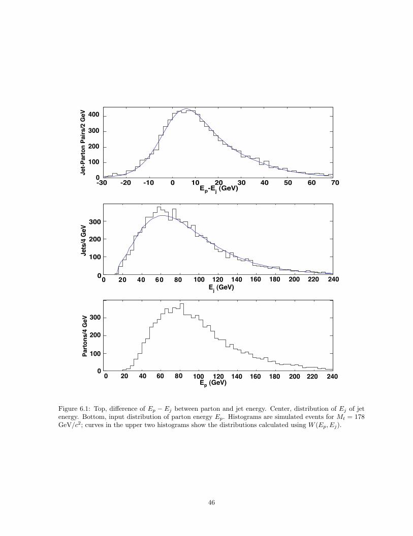
Jet-P
arto
n Pa
irs/2
GeV
0
100
200
300
400
(GeV)j-EpE-30 -20 -10 0 10 20 30 40 50 60 70
Jets/
4 GeV
0
100
200
300
0 20 40 60 8 1000 120 140 160 180 200 220 240 (GeV)jE
Parto
ns/4
GeV
0
100
200
300
(GeV)pE0 20 40 60 8 100 140 160 180 200 220 2400 120
Figure 6.1: Top, difference of Ep − Ej between parton and jet energy. Center, distribution of Ej of jetenergy. Bottom, input distribution of parton energy Ep. Histograms are simulated events for Mt = 178GeV/c2; curves in the upper two histograms show the distributions calculated using W (Ep, Ej).
46

<60) [GeV]p (10<EjE0 50 100 150 200 250 300
Jets
/10
GeV
050
100150200250300350400
<80) [GeV]p (60<EjE0 50 100 150 200 250 300
Jets
/10
GeV
0
100
200
300
400
500
<100) [GeV]p (80<EjE0 50 100 150 200 250 300
Jets
/10
GeV
050
100150200250300350400
<120) [GeV]p (100<EjE0 50 100 150 200 250 300
Jets
/10
GeV
0
50
100
150
200
250
<150) [GeV]p (120<EjE0 50 100 150 200 250 300
Jets
/10
GeV
020406080
100120140160180
<180) [GeV]p (150<EjE0 50 100 150 200 250 300
Jets
/10
GeV
0
20
40
60
80
100
Figure 6.2: Comparison of simulated Ej with calculations from W (Ep, Ej) from six ranges of Ep. His-tograms are simulated events; curves show the calculated distributions using W (Ep, Ej).
(GeV)jE0 40 80 120 160 200 240
stnevE
0
20
40
60
80
100
(GeV)jE0 40 80 120 160 200 240
stnevE
0
20
40
60
80
100
(GeV)jE0 40 80 120 160 200 240
stn evE
0102030405060708090
(GeV)jE0 40 80 120 160 200 240
stn evE
0102030405060708090
(GeV)jE0 40 80 120 160 200 240
stne vE
010
203040
5060
7080
(GeV)jE0 40 80 120 160 200 240
stne v E
0
10
20
30
40
50
60
70
80
Mt=150GeV/c Mt=160GeV/c Mt=170GeV/c
Mt=180GeV/c Mt=190GeV/c Mt=200GeV/c
2 2
22 2
2
Figure 6.3: Comparison of simulated Ej with calculations from W (Ep, Ej) from distributions Ep insimulated samples with Mt = 150, 160, 170, 180, 190, and 200 GeV/c2. Histograms are simulated eventsfor Mt = 178 GeV/c2; lines show the calculated distributions using Wj(Ep, Ej) derived using partonsfrom Mt = 178 GeV/c2.
47

6.2 tt pT Transfer Functions
Often in tt events, gluon radiation in an event will result in the tt system recoiling
and obtaining non-negligible pT . Correct reconstruction of the final state would require
knowledge of the tt pT . While we cannot measure the pT of the the tt (pttT ) system in
data events, we observe strong correlations between several measured quantities and pttT .
Gluons resulting from radiation, if energetic enough, can result in hadronic jets being
reconstructed in the event. Thus, for events with more than two jets passing our selection
cuts, we can utilize the measured jet energy of sub-leading jets to form transfer functions
to pttT . In Monte Carlo events, ptt
T is shown to have a strong dependence on the number of
jets in the event (see Figure 6.4). In addition, less energetic gluons resulting from radiation
may still deposit measured energy in the hadronic calorimeter. This softer energy can
be quantified using unclustered energy. The unclustered energy in an event is the total
energy in an event that is measured in the calorimeter, but not clustered into an object
such as a lepton or jet that is used in this measurement. The transverse components of
unclustered energy can be calculated as:
Eunclustered(x,y) =
∑i
(Li(x,y)+ ji(x,y)
)− 6ET (x,y) (6.6)
by subtracting the measured 6ET from the measured transverse energies of clustered ob-
jects passing the selection cuts outlined in Chapter 4 in an event. A comparison of the
transverse unclustered energy between what is measured in the data events used in this
analysis and what is predicted using Monte Carlo events is shown in Figure A.11.
For forming a transfer function for pttT , we utilize a variable U , whose transverse quan-
tities are given by:
U(x,y) = Eunclustered(x,y) +
Njets∑i=3
ji(x,y),
48
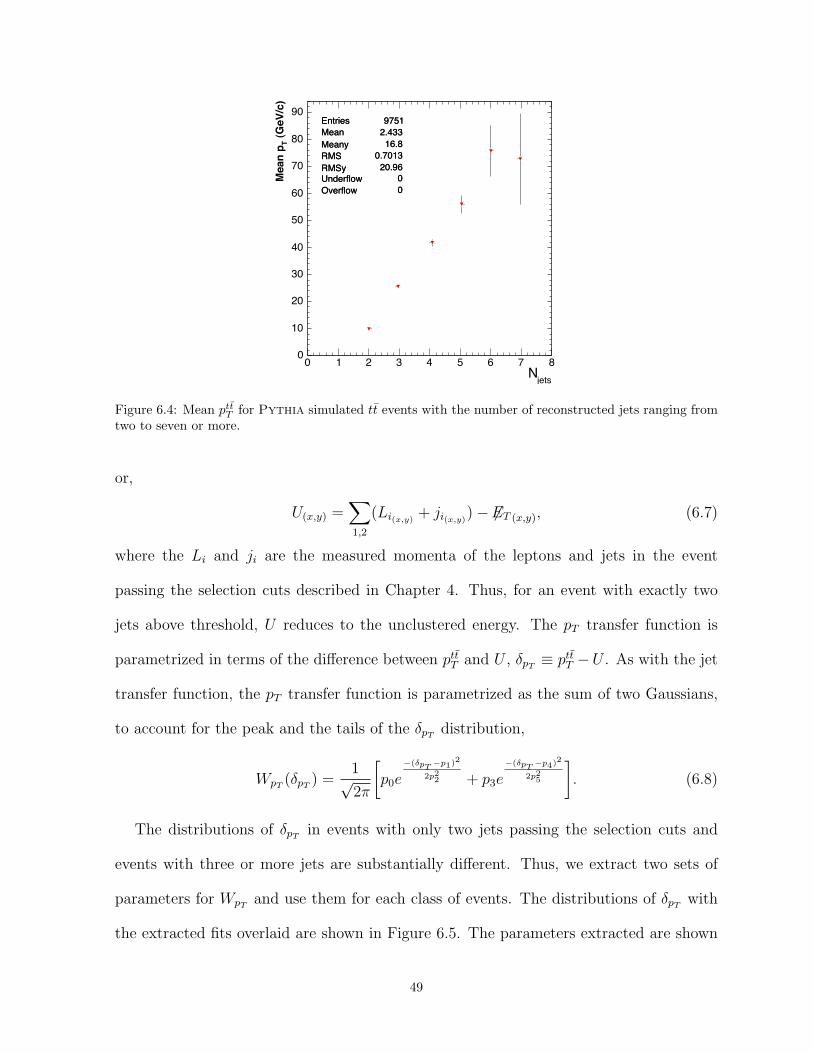
Entries 9751Mean 2.433Meany 16.8RMS 0.7013RMSy 20.96Underflow 0Overflow 0
jetsN0 1 2 3 4 5 6 7 8
(GeV
/c)
TM
ean
p
0
10
20
30
40
50
60
70
80
90Entries 9751Mean 2.433Meany 16.8RMS 0.7013RMSy 20.96Underflow 0Overflow 0
Figure 6.4: Mean pttT for Pythia simulated tt events with the number of reconstructed jets ranging from
two to seven or more.
or,
U(x,y) =∑1,2
(Li(x,y)+ ji(x,y)
)− 6ET (x,y), (6.7)
where the Li and ji are the measured momenta of the leptons and jets in the event
passing the selection cuts described in Chapter 4. Thus, for an event with exactly two
jets above threshold, U reduces to the unclustered energy. The pT transfer function is
parametrized in terms of the difference between pttT and U , δpT
≡ pttT −U . As with the jet
transfer function, the pT transfer function is parametrized as the sum of two Gaussians,
to account for the peak and the tails of the δpTdistribution,
WpT(δpT
) =1√2π
[p0e
−(δpT−p1)2
2p22 + p3e
−(δpT−p4)2
2p25
]. (6.8)
The distributions of δpTin events with only two jets passing the selection cuts and
events with three or more jets are substantially different. Thus, we extract two sets of
parameters for WpTand use them for each class of events. The distributions of δpT
with
the extracted fits overlaid are shown in Figure 6.5. The parameters extracted are shown
49

Top Mass Meeting, 6/14/06 Bo Jayatilaka
pT Transfer Functions
21
Entries 3249
Mean -0.06813
RMS 21.79
Underflow 0
Overflow 38
-100 -80 -60 -40 -20 0 20 40 60 80 1000
50
100
150
200
250
300Entries 3249
Mean -0.06813
RMS 21.79
Underflow 0
Overflow 38
T p!
Entries 6463
Mean -2.755
RMS 15.33
Underflow 20
Overflow 37
-100 -80 -60 -40 -20 0 20 40 60 80 1000
200
400
600
800
1000
1200
1400
1600
Entries 6463
Mean -2.755
RMS 15.33
Underflow 20
Overflow 37
2-jet onlyT p! =2 jets >2 jets
U - pT (GeV) U - pT (GeV)
• Plots show difference between ttbar pT and U
• Fitted TF is two GaussiansFigure 6.5: The distributions of δpTfor events with more than two jets (right) and exactly two jets (left).
The extracted fits are overlaid with the individual Gaussians in black and the total fit in red.
pi 2 jets >2 jetsp0 73.98 40.30p1 -9.351 GeV -2.321 GeVp2 26.80 GeV 38.89 GeVp3 1443 253.6p4 -0.597 GeV -7.202 GeVp5 5.568 GeV 14.27 GeV
Table 6.2: Parameters extracted for WpTusing tt Monte Carlo events. Events with 2 jets passing selection
cuts and events with more than 2 jets are considered separately.
in Table 6.2.
We form an additional transfer function which links the φ component of the tt mo-
mentum to the φ component of U . The φ transfer function, Wφ, is parametrized in terms
of δφ ≡ φtt − Uφ. As most events have U pointing opposite of the tt pT , we parametrize
this transfer function as the sum of a linear function and a Gaussian,
Wφ = p0 + p1δφ + p2e−(δφ−p3)2
2p24 . (6.9)
As with WpT, the φ transfer function is also derived separately for events with exactly
two jets and events with three or more jets. The distributions of δφ for these two classes
50

(rad.)! "0 0.5 1 1.5 2 2.5 30
50
100
150
200
250
300
350
400
450>2 jets
(rad.)! "0 0.5 1 1.5 2 2.5 30
20
40
60
80
100
120
140
160
180
200
220 =2 jets
Figure 6.6: The distributions of δφ for events with more than two jets (right) and exactly two jets (left).The extracted fits are overlaid in red.
pi 2 jets >2 jetsp0 86.24 37.77p1 13.44 6.718p2 170.3 5.045× 10⁶
p3 2.924 11.69p4 1.778 1.932
Table 6.3: Parameters extracted for Wφ using tt Monte Carlo events. Events with 2 jets passing selectioncuts and events with more than 2 jets are considered separately.
of events are shown in Figure 6.6 along with the extracted fits. The parameters extracted
are shown in Table 6.3.
51

CHAPTER 7
Signal Probability
The probability Ps(x|Mt) describes the likelihood of a measured event x being consis-
tent with tt decay with a top quark pole mass of Mt. It is constructed as a convolution
of the transfer functions described in the previous chapter and a leading-order matrix
element for tt production and decay.
7.1 Differential Cross-Section Expression
The probability density for qq → tt → b`ν`b`′ν`′ decays is constructed as the differential
cross section, dσ, with respect to the measured event quantities, x. The total cross section
σ is written as
σ =
∫ ∑a,b
(2π)4|M|2
4√
(q1 · q2)2 −m21m
22
faPDF
(qz1
Ebeam
)f bPDF
(qz2
Ebeam
)dΦ6dq1dq2, (7.1)
where the sum runs over incoming parton flavors,M is the matrix element for the process,
q1,2 and m1,2 refer to the momenta and mass of the incoming partons, fPDF are the parton
distribution functions for flavor a, and the integration is over the phase space for the six
final state particles as well as the longitudinal momenta of the incoming particles.
The matrix element [44, 45] has the form
|M|2 =g4
s
9FF
((2− β2s2
qt)−Xsc
), (7.2)
52

where β is the top-quark velocity in the qq rest frame, Xsc contains terms describing spin
correlations between the top quarks, gs is the strong coupling constant (g2s/4π = αs), sqt
is the sine of the angle between the incoming parton and the top quark, and F and F are
the propagators for the top and the anti-top respectively. We drop the spin correlation
term Xsc as it is negligible. The top-quark propagator and decay terms are given by
F =g4
w
4
[m2
t −m2¯ν
(m2t −M2
t )2 + (MtΓt)2
] [m2
t (1− c2¯b) + m2
¯ν(1 + c¯b)
2
(m2¯ν−M2
W )2 + (MW ΓW )2
], (7.3)
where mt is the invariant mass of the t-quark decay products and cij is the cosine of the
angle between particles i and j in the W rest frame. The Mt, Γt, MW , ΓW are the pole
masses and widths of the top-quark and W -boson, and gw1 is the weak coupling constant.
The top width, Γt [46], is a function of Mt, MW and ΓW as described by the standard
model to leading order:
Γt =GF M3
t |Vtb|2
8π√
2
[1− 3
M4W
M4t
+ 2M6
W
M6t
+ · · ·]
, (7.4)
where GF is the Fermi coupling constant and |Vtb| is a mixing term from the CKM
matrix. F is given by the same expression as Eq. 7.3, replacing the terms for t and its
decay products with t and its decay products.
While approximately 15% of tt pairs in pp collisions at√
s = 1.96 TeV are produced in
gluon-gluon fusion (gg → tt) [15], our studies have shown that this term can be excluded
from the matrix element with very little loss of sensitivity to the measurement2.
To evaluate the differential cross section with respect to observed quantities, dσdx
, we
introduce conditional probability terms that relate the observed quantities to the par-
ton level variables and subsequently integrate over unconstrained parton-level quantities,
as described above. In order to make the computation associated with these integrals1GF =
√2g2
w/8M2W
2Additionally, we can verify that the exclusion of the gg term introduces no bias by using simulated events with variedinitial state content and using only the qq matrix element. We observe negligible variation in the measured mass amongstsamples consisting of 0%, 5%, and 15% gg events.
53

tractable, a series of assumptions, listed in Chapter 5, are made regarding the transfer
between parton level quantities and the observables. These assumptions are enforced as
delta functions in the expression for the differential cross section.
The differential cross section is given by
dσ
dx=
(1
(2π)3
)6 ∫ ∑a,b
|M(qi1, q
j2 → `1, ν1, p1, `2, ν2, p2)|2(2π)4δ4(
∑k=1,2
(qk − `k − νk − pk))
× δ(qx1) δ(qy1) dqx1 dqy1δ(qx2) δ(qy2) dqx2 dqy2
(2π)4faPDF(q
iz1
/Ebeam) f bPDF(q
jz2
/Ebeam)dqi1 dqj
2
4√
(q1 · q2)2 −m2q1
m2q2
× δ3(`1 − L1) δ3(`2 − L2)d3`1
2E`1
d3`2
2E`2
δ(θp1 − θj1) δ(θp2 − θj2)δ(φp1 − φj1) δ(φp2 − φj2)
×W (Ep1 , Ej1)W (Ep2 , Ej2)WpT(ptt
T , U)Wφ(φtt, Uφ)d3p1
2Ep1
d3p2
2Ep2
d3ν1
2Eν1
d3ν2
2Eν2
dpttx dptt
y .
(7.5)
The sum is over possible incoming parton flavors. The term 1/4√
(q1 · q2)2 −m2q1
m2q2
reduces to fflux(qz1 , qz2) = 1/2qz1qz2 with the assumption that the parton mass is small
in comparison to the longitudinal momentum.
7.2 Phase Space Transformation and Integration
We integrate over the lepton momenta, initial parton momenta, intermediate top and
W momenta, angular components of the b-partons, the x and y components of the mo-
mentum of the tt system, and the six components of neutrino momenta.
In order to efficiently integrate over the parton-level variables, we perform a transfor-
mation which splits the original phase space into subspaces and introduces the equivalent
number of extra variables and integrations. We introduce invariant masses that corre-
spond to intermediate t and t quarks and W -bosons. Each additional integration over
an invariant mass of the intermediate particle has a corresponding δ-function in squared
invariant mass, and each intermediate particle four-momentum has corresponding δ4-
54
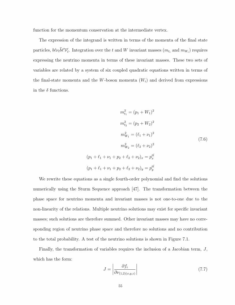
function for the momentum conservation at the intermediate vertex.
The expression of the integrand is written in terms of the momenta of the final state
particles, b`ν`b`′ν ′`. Integration over the t and W invariant masses (mti and mWi
) requires
expressing the neutrino momenta in terms of these invariant masses. These two sets of
variables are related by a system of six coupled quadratic equations written in terms of
the final-state momenta and the W -boson momenta (Wi) and derived from expressions
in the δ functions.
m2t1
= (p1 + W1)2
m2t2
= (p2 + W2)2
m2W1
= (`1 + ν1)2
m2W2
= (`2 + ν2)2
(p1 + `1 + ν1 + p2 + `2 + ν2)x = pttx
(p1 + `1 + ν1 + p2 + `2 + ν2)y = ptty
(7.6)
We rewrite these equations as a single fourth-order polynomial and find the solutions
numerically using the Sturm Sequence approach [47]. The transformation between the
phase space for neutrino momenta and invariant masses is not one-to-one due to the
non-linearity of the relations. Multiple neutrino solutions may exist for specific invariant
masses; such solutions are therefore summed. Other invariant masses may have no corre-
sponding region of neutrino phase space and therefore no solutions and no contribution
to the total probability. A test of the neutrino solutions is shown in Figure 7.1.
Finally, the transformation of variables requires the inclusion of a Jacobian term, J ,
which has the form:
J =
∣∣∣∣ ∂fi
∂ν(1,2)(x,y,z)
∣∣∣∣ (7.7)
55

Entries 5001Mean 0.02042RMS 0.7882
E!-50 -40 -30 -20 -10 0 10 20 30 40 500
500
1000
1500
2000
2500
3000
3500Entries 5001Mean 0.02042RMS 0.7882
E residual"
Figure 7.1: A plot of the difference between the true neutrino energy and neutrino energy as solved fromequation 7.6 in simulated events using parton-level quantities.
The fi are the functions of neutrino momenta that occur inside δ-functions:
f1 =((L1 + ν1 + p1)x + (L2 + ν2 + p2)x − ptt
x
)f2 =
((L1 + ν1 + p1)y + (L2 + ν2 + p2)y − ptt
y
)f3 =
((L1 + ν1 + p1)
2 −M2t1
)f4 =
((L2 + ν2 + p2)
2 −M2t2
)f5 =
((L1 + ν1)
2 −M2W1
)f6 =
((L2 + ν2)
2 −M2W2
)
(7.8)
The determinant has the form: ∣∣∣∣∣∣∣∣∣∣∣∣∣∣∣∣∣∣∣∣∣∣
1 0 J3x 0 J5x 0
0 1 J3y 0 J5y 0
0 0 J3z 0 J5z 0
1 0 0 J4x 0 J6x
0 1 0 J4y 0 J6y
0 0 0 J4z 0 J6z
∣∣∣∣∣∣∣∣∣∣∣∣∣∣∣∣∣∣∣∣∣∣56

that evaluates to:
J = |J3zJ4zJ5yJ6x − J3yJ4zJ5zJ6x − J3zJ4zJ5xJ6y+
+ J3xJ4zJ5zJ6y + J3zJ4yJ5xJ6z − J3zJ4xJ5yJ6z+
+ J3yJ4xJ5zJ6z − J3xJ4yJ5zJ6z|
(7.9)
with:
J3x =∂f3
∂ν1x
=2(L0
1 + p01)ν1x√
ν21x + ν2
1y + ν21z
− 2(L1x + p1x)
J3y =∂f3
∂ν1y
=2(L0
1 + p01)ν1y√
ν21x + ν2
1y + ν21z
− 2(L1y + p1y)
J3z =∂f3
∂ν1z
=2(L0
1 + p01)ν1z√
ν21x + ν2
1y + ν21z
− 2(L1z + p1z)
J4x =∂f4
∂ν2x
=2(L0
2 + p02)ν2x√
ν22x + ν2
2y + ν22z
− 2(L2x + p2x)
J4y =∂f4
∂ν2y
=2(L0
2 + p02)ν2y√
ν22x + ν2
2y + ν22z
− 2(L2y + p2y)
J4z =∂f4
∂ν2z
=2(L0
2 + p02)ν2z√
ν22x + ν2
2y + ν22z
− 2(L2z + p2z)
J5x =∂f5
∂ν1x
=2(L0
1ν1x)√ν2
1x + ν21y + ν2
1z
− 2L1x
J5y =∂f5
∂ν1y
=2(L0
1ν1y)√ν2
1x + ν21y + ν2
1z
− 2L1y
J5z =∂f5
∂ν1z
=2(L0
1ν1z)√ν2
1x + ν21y + ν2
1z
− 2L1z
J6x =∂f6
∂ν2x
=2(L0
2ν2x)√ν2
2x + ν22y + ν2
2z
− 2L2x
J6y =∂f6
∂ν2y
=2(L0
2ν2y)√ν2
2x + ν22y + ν2
2z
− 2L2y
J6z =∂f6
∂ν2z
=2(L0
2ν2z)√ν2
2x + ν22y + ν2
2z
− 2L2z
(7.10)
57
The final form of the expression is
dσ
dx=
(1
(2π)3
)6
(2π)2
∫ ∑a,b
|M|2
2E2beam
J−1
Eν1Eν2EL1EL2
|p1|2 sin θp1d|p1|2Ep1
|p2|2 sin θp2d|p2|2Ep2
×faPDF
(qz1
Ebeam
)f bPDF
(qz2
Ebeam
)fflux(qz1 , qz2)W (Ep1 , Ej1) W (Ep2 , Ej2)
×WpT(ptt
T , U)Wφ(φtt, Uφ) |pttT | dptt
T dφttMt1 Mt2 MW1 MW2 dMt1 dMt2 dMW1 dMW2 ,
(7.11)
where the remaining integrations are over the invariant masses of the t quarks and the W
bosons, the magnitude and φ direction of pttT , and the magnitude of the b-quark momenta.
The cross section as a function of Mt is expressed as a eight-dimensional integral; this
integration is performed numerically using the Vegas [48] algorithm as implemented in
the GNU Scientific Library [49]. As we do not have a priori knowledge of which jet and
which lepton came from the same top quark, we evaluate the final probability for each of
the two possible combinations and sum the two resulting probabilities.
7.3 Tests of the Signal Probability
We can test the signal probability using simulated events using increasing levels of
complexity.
We begin with simulated pp → tt events generated with Pythia in which all of the
parton-level information from the hard scattering and subsequent decay is known. Evalu-
ating the matrix element in Equation 7.2 for these events as a function of top quark pole
mass results in sharp peaks at the invariant mass of each of the top quarks in the event,
as shown in Figure 7.2.
We can then discard information not present in data events (such as neutrino momenta)
and apply Gaussian smearing to b-quark energies to simulate jets. We then evaluate the
58

172 174 176 178 180 182 1840
2000
4000
6000
8000
10000
12000
14000
172 174 176 178 180 182 1840
20
40
60
80
100
120
140
160
180
172 174 176 178 180 182 1840
100
200
300
400
500
600
172 174 176 178 180 182 1840
20
40
60
80
100
120
140
160
180
172 174 176 178 180 182 1840
20
40
60
80
100
120
140
160
172 174 176 178 180 182 1840
50
100
150
200
250
172 174 176 178 180 182 1840
1000
2000
3000
4000
5000
6000
7000
8000
172 174 176 178 180 182 1840
20
40
60
80
100
120
140
160
172 174 176 178 180 182 1840
20
40
60
80
100
120
140
160
Mt(GeV/c2) Mt(GeV/c2)
Mt(GeV/c2) Mt(GeV/c2)
|M|2
|M|2
|M|2
|M|2
Figure 7.2: Evaluation of the tt matrix element using parton-level information from Monte Carlo events.
integral in Equation 7.11, resulting in curves as shown in Figure 7.3. The resulting curves
are smooth, indicating that the calculation is well-behaved, and peak roughly in the region
corresponding to the true invariant masses.
As individual events are not very illustrative, we then perform pseudo-experiments
with ensembles of simulated events. The mass is extracted from each pseudo-experiment
using the same method as is used with data events (see Chapter 9). The distribution of
pulls of each pseudo-experiment gives a measure of how well the statistical uncertainty is
estimated. The pull of a pseudo-experiment is defined as
p =Mmeas
t −M truet
σMt
, (7.12)
where Mmeast is the mass measured in each pseudo-experiment, M true
t is the input mass
and σMt is the measured statistical uncertainty in each pseudo-experiment. For a set of
pseudo-experiments where the result is unbiased and the error is estimated correctly, the
59

140 160 180 200 2200
0.2
0.4
0.6
0.8
1
1.2
1.4
1.6
1.8
2
140 160 180 200 2200
0.2
0.4
0.6
0.8
1
1.2
140 160 180 200 2200
2
4
6
8
10
140 160 180 200 2200
2
4
6
8
10
12
14
16
18
20
22
140 160 180 200 2200
5
10
15
20
25
30
35
40
140 160 180 200 2200
0.02
0.04
0.06
0.08
0.1
0.12
0.14
0.16
0.18
0.2
0.22
0.24
140 160 180 200 2200
0.1
0.2
0.3
0.4
0.5
0.6
140 160 180 200 2200
5
10
15
20
25
30
140 160 180 200 2200
0.1
0.2
0.3
0.4
0.5
0.6
Mt(GeV/c2) Mt(GeV/c2)
Mt(GeV/c2) Mt(GeV/c2)
Ps
Ps
Ps
Ps
Figure 7.3: Evaluation of Ps using Monte Carlo events with smeared partons.
Events True Mass Mean Mass Mass RMS Pull WidthSmeared Parton 178 176.7± 1.5 5.5 1.04± 0.04Fully Simulated 178 178.3± 1.0 8.7 1.14± 0.04
Table 7.1: Results from pseudo-experiments using both smeared parton-level quantities and fully simu-lated events and the full signal probability to extract the measured mass.
pulls are expected to fall in a gaussian distribution with a mean of 0 and a width of 1.0.
We perform pseudo-experiments using parton level quantities with smeared b-quarks
as above and also using events passed through a full detector simulation. The results
of these pseudo-experiments are shown in Table 7.1. We note that the pull widths of
the fully simulated events, which we expect to be similar to events observed in the data,
indicate the statistical uncertainty is underestimated by approximately 15%. This is due
to the violation of the assumptions listed in Chapter 5 in these events. These assumptions
are all held in smeared parton-level events, where the pull width is consistent with 1.0.
This indicates the method correctly estimates the statistical uncertainty in the class of
60

events where all assumptions made are held. We can study the effect of each of these
assumptions by performing pseudo-experiments where we control the degree to which the
assumptions are violated in the events used.
7.3.1 Jet-Parton Assignment
In samples of simulated events which pass selection requirements, 70% of events con-
tain two reconstructed jets whose axes lie within a cone of ∆R < 0.7 of unique b-quarks
from the top quark decay. Monte Carlo experiments using this subset of events have a
significantly smaller pull width, 1.06 ± 0.04. This suggests that events in which the as-
sumption of correspondence between jets and b-quarks is violated contribute significantly
to non-unit pull widths.
7.3.2 Lepton Resolution
Though lepton energies are well measured by CDF, electrons and muons are measured
by different subdetectors. The energy of electrons at high ET is very well measured by
the calorimeter:
σE
E=
13.5%√E(GeV)
⊕ 2.0%. (7.13)
The momentum of muons is measured by the central tracker, whose resolution begins to
degrade at large pT :
σpT
pT
= 0.0011 · pT (GeV/c). (7.14)
Monte Carlo experiments formed using events in which jets are matched well to b-quarks
and events containing only electrons have a pull width of 0.98 ± 0.04. Similar Monte
Carlo experiments using only muons have a pull width of 1.03 ± 0.04, indicating that
muon momentum resolution contributes to pull widths greater than unity. Electrons and
61
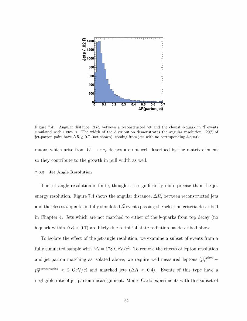
Δ
Figure 7.4: Angular distance, ∆R, between a reconstructed jet and the closest b-quark in tt eventssimulated with herwig. The width of the distribution demonstrates the angular resolution. 20% ofjet-parton pairs have ∆R ≥ 0.7 (not shown), coming from jets with no corresponding b-quark.
muons which arise from W → τντ decays are not well described by the matrix-element
so they contribute to the growth in pull width as well.
7.3.3 Jet Angle Resolution
The jet angle resolution is finite, though it is significantly more precise than the jet
energy resolution. Figure 7.4 shows the angular distance, ∆R, between reconstructed jets
and the closest b-quarks in fully simulated tt events passing the selection criteria described
in Chapter 4. Jets which are not matched to either of the b-quarks from top decay (no
b-quark within ∆R < 0.7) are likely due to initial state radiation, as described above.
To isolate the effect of the jet-angle resolution, we examine a subset of events from a
fully simulated sample with Mt = 178 GeV/c2. To remove the effects of lepton resolution
and jet-parton matching as isolated above, we require well measured leptons (pleptonT −
preconstructedT < 2 GeV/c) and matched jets (∆R < 0.4). Events of this type have a
negligible rate of jet-parton misassignment. Monte Carlo experiments with this subset of
62

events have a pull width of 1.04±0.04, consistent with experiments described above which
use only electrons and matched jets. Further tightening the ∆R requirement reduces the
pull width to 0.97± 0.04.
As we observe the underestimation of the statistical uncertainty in fully simulated
events to be constant as a function of input top quark mass, we can apply a constant
scale factor to the measured uncertainty. This procedure is described in Chapter 9.
63

CHAPTER 8
Background Probabilities
We calculate the per-event differential cross section for the three largest sources of
background: the Z/γ∗ + 2 jet process (Zjj) where the Z decays directly to electrons or
muons, the WW + 2 jet process (WWjj) and the W + 3 jet process (Wjjj) where one
jet is misidentified as a lepton. WZ with associated jets and Z → ττ with two jets have
a small overall contribution to the sample and are not directly modeled.
8.1 Matrix Element Evaluation
Unlike top pair production, the major background processes can not be well described
using a small number of diagrams. This is primarily due to the fact that more diagrams are
needed to describe the presence of hard jets in these background events. In addition, there
is no closed-form expression for the QCD processes which dominate the jet production in
these background events.
We therefore adapt routines from the Alpgen Monte Carlo generator, which make
effective approximations to evaluate the matrix elements for these processes. While gen-
erators such as CompHEP [50] and Madgraph [51] provide generation based directly
on the explicit evaluation of the Feynman diagrams, final states with more than a single
jet result in the calculation becoming unwieldy and slow.
64

The Alpgen routines are a function of the spin and color configurations of the initial
and final state partons as well as their momenta. While it is computationally prohibitive to
rigorously sum over each of the possible configurations, it is possible to employ statistical
sampling to numerically evaluate the average matrix element, M. Figure 8.1 shows the
distribution of |M|2 in generated events using sums of a specific number of terms; it
is clear that the matrix element calculation is sensitive to the configuration and that it
converges fairly rapidly.
We sample spin and color configurations until the sum has converged, satisfying the
criteria
RMS(|M|2)Mean(|M|2)
√N
< ε (8.1)
where ε is the convergence tolerance, set to ε = 0.25 for these calculations, and N is the
number of terms summed over.
The calculation of the matrix element is well behaved; as an example, Figure 8.2 shows
the variation of |MZjj|2 with the invariant mass of the lepton pair in Z → `` events. It
shows the expected strong peak at Mll = MZ .
The final measurement is calibrated using fully realistic Monte Carlo events, which will
incorporate the effects of these approximations.
8.2 Z/γ∗ + 2 jets
We employ the set of assumptions as described in Chapter 5 and use transfer functions
as defined and derived in Chapter 6 to connect the parton-level quantities to observed
quantities. We integrate over the unknown pT which arises from additional softer jets and
unclustered energy. We express this as rx and ry, components of the recoil in the x and
y axes, respectively. We integrate over drxdry using uncorrelated Gaussian priors in x
65

)2
log(|M|!-10 -8 -6 -4 -2 0 2 4 6 8 10
Events
1
10
)2
log(|M|!-10 -8 -6 -4 -2 0 2 4 6 8 10
Events
1
10
)2
log(|M|!-10 -8 -6 -4 -2 0 2 4 6 8 10
Events
1
10
)2
log(|M|!-10 -8 -6 -4 -2 0 2 4 6 8 10
Events
1
10
210
)2
log(|M|!-10 -8 -6 -4 -2 0 2 4 6 8 10
Events
1
10
210
)2
log(|M|!-10 -8 -6 -4 -2 0 2 4 6 8 10
Events
1
10
210
)2
log(|M|!-10 -8 -6 -4 -2 0 2 4 6 8 10
Events
1
10
)2
log(|M|!-10 -8 -6 -4 -2 0 2 4 6 8 10
Events
1
10
)2
log(|M|!-10 -8 -6 -4 -2 0 2 4 6 8 10
Events
1
10
210
)2
log(|M|!-10 -8 -6 -4 -2 0 2 4 6 8 10
Events
1
10
210
)2
log(|M|!-10 -8 -6 -4 -2 0 2 4 6 8 10
Events
1
10
210
)2
log(|M|!-10 -8 -6 -4 -2 0 2 4 6 8 10
Events
1
10
210
)2
log(|M|!-10 -8 -6 -4 -2 0 2 4 6 8 10
Events
1
10
)2
log(|M|!-10 -8 -6 -4 -2 0 2 4 6 8 10
Events
1
10
)2
log(|M|!-10 -8 -6 -4 -2 0 2 4 6 8 10
Events
1
10
210
)2
log(|M|!-10 -8 -6 -4 -2 0 2 4 6 8 10
Events
1
10
210
)2
log(|M|!-10 -8 -6 -4 -2 0 2 4 6 8 10
Events
1
10
210
)2
log(|M|!-10 -8 -6 -4 -2 0 2 4 6 8 10
Events
1
10
210
)2
log(|M|!-10 -8 -6 -4 -2 0 2 4 6 8 10
Events
1
10
)2
log(|M|!-10 -8 -6 -4 -2 0 2 4 6 8 10
Events
1
10
)2
log(|M|!-10 -8 -6 -4 -2 0 2 4 6 8 10
Events
1
10
210
)2
log(|M|!-10 -8 -6 -4 -2 0 2 4 6 8 10
Events
1
10
210
)2
log(|M|!-10 -8 -6 -4 -2 0 2 4 6 8 10
Events
1
10
210
)2
log(|M|!-10 -8 -6 -4 -2 0 2 4 6 8 10
Events
1
10
210
)2
log(|M|!-10 -8 -6 -4 -2 0 2 4 6 8 10
Events
1
10
)2
log(|M|!-10 -8 -6 -4 -2 0 2 4 6 8 10
Events
1
10
)2
log(|M|!-10 -8 -6 -4 -2 0 2 4 6 8 10
Events
1
10
210
)2
log(|M|!-10 -8 -6 -4 -2 0 2 4 6 8 10
Events
1
10
210
)2
log(|M|!-10 -8 -6 -4 -2 0 2 4 6 8 10
Events
1
10
210
)2
log(|M|!-10 -8 -6 -4 -2 0 2 4 6 8 10
Events
1
10
210
)2
log(|M|!-10 -8 -6 -4 -2 0 2 4 6 8 10
Events
1
10
)2
log(|M|!-10 -8 -6 -4 -2 0 2 4 6 8 10
Events
1
10
210
)2
log(|M|!-10 -8 -6 -4 -2 0 2 4 6 8 10
Events
1
10
210
)2
log(|M|!-10 -8 -6 -4 -2 0 2 4 6 8 10
Events
1
10
210
)2
log(|M|!-10 -8 -6 -4 -2 0 2 4 6 8 10
Events
1
10
210
)2
log(|M|!-10 -8 -6 -4 -2 0 2 4 6 8 10
Events
1
10
210
Figure 8.1: Variation in log(|M |2) with increasing number of terms in the spin and color sum. Fromtop, moving downwards, the number of spin terms sampled increases by powers of 2 from 1 to 32. Fromleft, moving right, the number of color terms sampled increases by powers of 2 from 1 to 32.
66
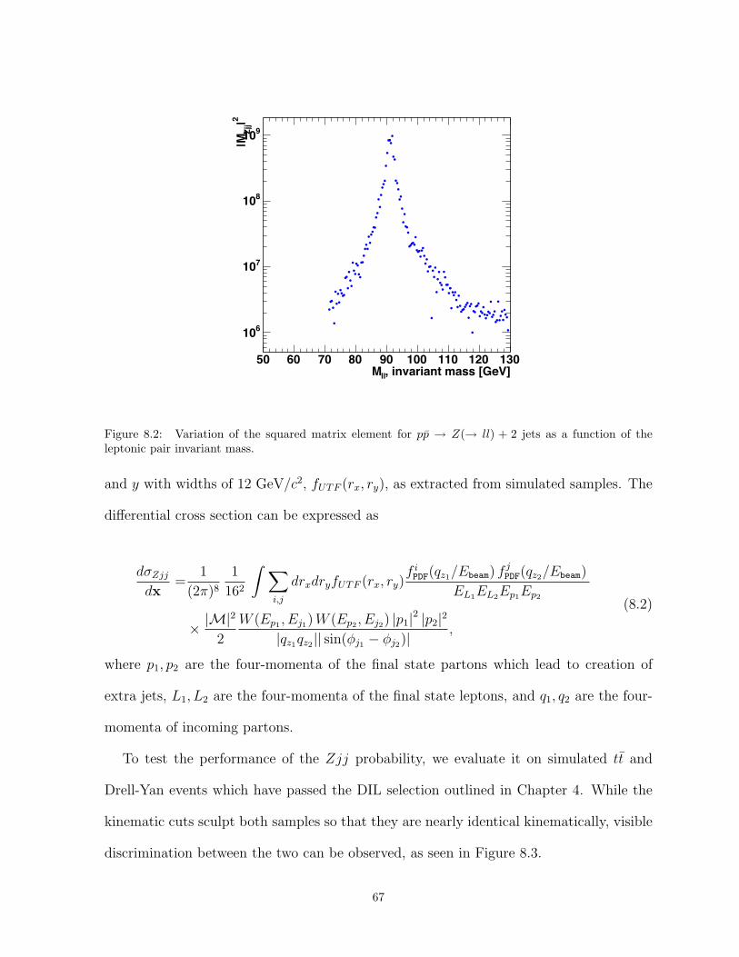
, invariant mass [GeV]llM50 60 70 80 90 100 110 120 130
2 |Zj
j|M
610
710
810
910
Figure 8.2: Variation of the squared matrix element for pp → Z(→ ll) + 2 jets as a function of theleptonic pair invariant mass.
and y with widths of 12 GeV/c2, fUTF (rx, ry), as extracted from simulated samples. The
differential cross section can be expressed as
dσZjj
dx=
1
(2π)8
1
162
∫ ∑i,j
drxdryfUTF (rx, ry)f iPDF(qz1/Ebeam) f j
PDF(qz2/Ebeam)
EL1EL2Ep1Ep2
× |M|2
2
W (Ep1 , Ej1) W (Ep2 , Ej2) |p1|2 |p2|2
|qz1qz2|| sin(φj1 − φj2)|,
(8.2)
where p1, p2 are the four-momenta of the final state partons which lead to creation of
extra jets, L1, L2 are the four-momenta of the final state leptons, and q1, q2 are the four-
momenta of incoming partons.
To test the performance of the Zjj probability, we evaluate it on simulated tt and
Drell-Yan events which have passed the DIL selection outlined in Chapter 4. While the
kinematic cuts sculpt both samples so that they are nearly identical kinematically, visible
discrimination between the two can be observed, as seen in Figure 8.3.
67

(Zjj)/dx ]!ln[ d-90 -80 -70 -60 -50 -40 -30 -20 -100
0.020.04
0.060.08
0.10.12
0.140.16
0.18
0.20.22 tt
Z+2p
Figure 8.3: Evaluation of the Zjj probability for fully reconstructed Z and tt events, after selection isapplied.
8.3 WW + 2 jets
The production of W pairs with associated jets is modeled in a similar fashion. We
make the assumptions listed in Chapter 5 and in addition assume that the pT of the
system is 0. We choose to transform the phase-space by introducing the invariant masses
of the intermediate W bosons. We express all the parton variables except the neutrino
momenta in spherical coordinates. Integrating over delta functions for lepton energy, jet
angles, and total conservation of momentum gives
dσWWjj
dx=
1
(2π)16
∫ ∑a,b
|M|2
2E2beam
|p1|2 sin θp1d|p1|2Ep1
|p2|2 sin θp2d|p2|2Ep2
J−1
Eν1Eν2EL1EL2
× faPDF
(qz1
Ebeam
)f bPDF
(qz2
Ebeam
)fflux(qz1 , qz2)W (Ep1 , Ej1) W (Ep2 , Ej2)
×MW1 MW2 dMW1 dMW2dν1zdν2z,
(8.3)
68

where L1, L2 are the measured four-momenta , `1, `2 are the parton-level four-momenta
of the final state leptons, ν1, ν2 are the four-momenta of the final state neutrinos, p1, p2
are the four-momenta of the final state partons that lead to creating extra jets, and q1, q2
are the four-momenta of the incoming partons. The sum runs over the incoming parton
flavors.
The final integration is performed over the momenta of the partons which lead to jet
production, the W boson invariant masses, and the z components of neutrino momenta.
Transformation of the space requires solving a coupled system of equations to express the
neutrino energies in terms of the W masses and the evaluation of a Jacobian, J , similar
to the signal probability.
An evaluation of the Alpgen matrix element for WWjj is shown in Figure 8.4 (left)
using generated, parton-level events for both WWjj and tt. We also evaluate the WWjj
probability on simulated events that have passed final dilepton selections for the DIL
sample. As with the Zjj case, the event selection results in the passing background
events being very similar to tt kinematically. There is still, however, visible discrimination
between WWjj events and tt events using the WWjj probability calculation, as seen in
Figure 8.4 (right).
8.4 Fakes
Events in which a jet is misidentified as a lepton can be modeled with the process
pp → Wjjj → lνjjj. Using this process as the basis for the model, we sum over the
possibility that either lepton is a fake originating from a jet:
Pfake = PWjjj(j1, j2, l1, [l2 → j3]) + PWjjj(j1, j2, [l1 → j3], l2). (8.4)
Making the assumptions listed in Chapter 5 and in addition assuming that the pT of
69
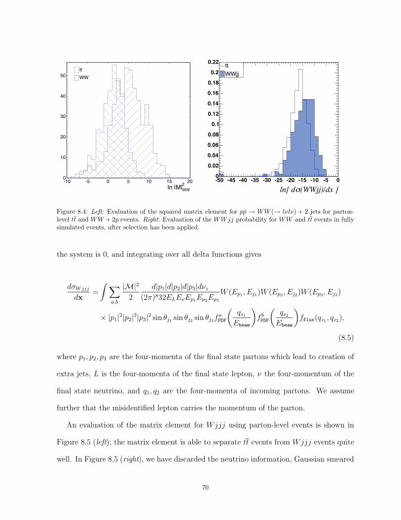
2
WWln |M|
-10 -5 0 5 10 15 200
10
20
30
40
50
tt
WW
(WWjj)/dx ]!ln[ d
-50 -45 -40 -35 -30 -25 -20 -15 -10 -5 00
0.02
0.04
0.06
0.08
0.1
0.12
0.14
0.16
0.18
0.2
0.22tt
WWjj
Figure 8.4: Left: Evaluation of the squared matrix element for pp → WW (→ lνlν) + 2 jets for parton-level tt and WW +2p events. Right: Evaluation of the WWjj probability for WW and tt events in fullysimulated events, after selection has been applied.
the system is 0, and integrating over all delta functions gives
dσWjjj
dx=
∫ ∑a,b
|M|2
2
d|p1|d|p2|d|p3|dνz
(2π)832ELEνEp1Ep2Ep3
W (Ep1 , Ej1)W (Ep2 , Ej2)W (Ep3 , Ej3)
× |p1|2|p2|2|p3|2 sin θj1 sin θj2 sin θj3faPDF
(qz1
Ebeam
)f bPDF
(qz2
Ebeam
)fflux(qz1 , qz2),
(8.5)
where p1, p2, p3 are the four-momenta of the final state partons which lead to creation of
extra jets, L is the four-momenta of the final state lepton, ν the four-momentum of the
final state neutrino, and q1, q2 are the four-momenta of incoming partons. We assume
further that the misidentified lepton carries the momentum of the parton.
An evaluation of the matrix element for Wjjj using parton-level events is shown in
Figure 8.5 (left); the matrix element is able to separate tt events from Wjjj events quite
well. In Figure 8.5 (right), we have discarded the neutrino information, Gaussian smeared
70

the parton-level quantities and performed the four-dimensional integration using Gaussian
transfer functions.
Finally, we evaluate the full fake probability, applying the integration and transfer
functions as above. We employ a sample of events from the data which are candidates to
produce a fake lepton. Figure 8.6 shows the resulting distributions.
2|
Wjjj|ME
-20 -15 -10 -5 0 5 10
Events
0
0.05
0.1
0.15
0.2
0.25
ttbar
W+3p
/dxWjjj
!d-70 -65 -60 -55 -50 -45 -40 -35 -30
Events
0
0.05
0.1
0.15
0.2
0.25 ttbar
W+3p
Figure 8.5: Left: Evaluation of the squared matrix element for pp → W (→ lν) + 3 jets for parton-leveltt and W + 3p events. Right: Evaluation of the Wjjj probability for Gaussian smeared Wjjj and ttevents.
71

(Wjjj)/dx ]!ln[ d-80 -70 -60 -50 -40 -30 -20 -10 00
0.1
0.2
0.3
0.4
0.5 ttFakes
Figure 8.6: Evaluation of the Wjjj probability for fully simulated tt and events from the data which arecandidates to produce a fake lepton.
72

CHAPTER 9
Mass Extraction and Calibration
In this chapter, we discuss the combination of the per-event differential cross section
calculations for signal and background into a joint probability for a sample of events, the
procedure for mass extraction, and calibration of the method using simulated events.
9.1 Mass Extraction
9.1.1 Posterior Probability
We express the individual event probability density in x as a sum of the signal and
background probabilities with their respective fractions as in Equation 5.5. The signal
and background fractions are expressed in terms of the number of expected signal events
λs(Mt) and background λb events:
ps(Mt) =λs(Mt)
λs(Mt) + λb
pbi(Mt) =
λbi
λs(Mt) + λb
, (9.1)
where λb =∑
i λbi. The values used for λs(175) and the λbi
are given in Table 4.1. The
expected signal λs(Mt) is calculated relative to a reference point M0 and extrapolated to
73

other masses using the mass dependence of the total accepted cross section σs(Mt)εs(Mt):
λs(Mt) = λs(m0)σs(Mt)εs(Mt)
σs(M0)εs(M0), (9.2)
where σs(Mt) is the total production cross section [15] and εs(Mt) is the acceptance
measured in Monte Carlo events (see Figure 4.3).
For an individual event x, P (x|Mt) is a likelihood in Mt. The posterior probability
density in Mt is the product of a flat prior probability and the product of the individ-
ual event likelihoods. The measured mass, Mt, is chosen as the expectation value of
the posterior probability to avoid potential fluctuations in the position of the maximum
probability:
Mt =
∫dMtMtP (x|Mt)∫dMtP (x|Mt)
(9.3)
The measured statistical uncertainty, ∆Mt, is the standard deviation of the posterior
probability,
∆Mt =
√∫dMtM2
t P (x|Mt)∫dMtP (x|Mt)
− (Mt)2 (9.4)
Due to effects including the violation of assumptions listed in Chapter 5 in realistic
events, imperfections in the models used for background probabilities, and the presence
of backgrounds that are not modeled with a background probability, Mt and ∆Mt deviate
from what we expect the true mass and error to be. The following section describes the
procedure used to extract a calibration to correct for these effects.
9.2 Calibration
We have searched for any potential biases on the extracted mass or its uncertainty due
to our fitting procedure. We parameterize this bias using a linear correction factor to the
74

measured mass consisting of an offset M0 and a slope sMt ,
Mt = 178.0 GeV/c2 + (Mt −M0)/sMt , (9.5)
and a simple scale factor,
∆Mt = S∆ ×∆Mt/sMt , (9.6)
to the measured statistical error in data, where M0, sMt , S∆ are extracted from ensem-
bles of Monte Carlo experiments. In the following sections, we study the calibration of
the method in Monte Carlo experiments with only tt events as well as in Monte Carlo
experiments with both tt and background events.
9.2.1 Signal only tests with Ps
We first measure the response of the method using purely signal events. The number
of events in each Monte Carlo experiment is a random number, Poisson distributed with
expected number of events shown in Table 4.1. The probability expression in this case
includes only the term that describes leading order tt production. Figure 9.1 shows
that the response is linear, with a slope very close to 1.0. The statistical uncertainty is
underestimated due to approximations (listed in Chapter 5) made in the calculation of
the likelihood as discussed in detail in Chapter 7. Figure 9.2 shows the residual and pull
parameters.
9.2.2 Signal and Background tests with Ps
We then measure the response of the method using signal and background events.
The number of signal and background events in each Monte Carlo experiment is Poisson
distributed around the expected number shown in Table 4.1. The probability expression
only includes the term that describes the signal process and thus the sensitivity of the
method degrades considerably as seen in Figure 9.3.
75

)2 (GeV/ctTrue M155 160 165 170 175 180 185 190 195
)2 (GeV/ctTrue M155 160 165 170 175 180 185 190 195
)2 (G
eV/c
tM
easu
red
M
150
160
170
180
190
200
tHerwig t s×) 0-Mt178 + (M
0.2±=177.8 0M
0.02± s=1.04
Figure 9.1: Response for Monte Carlo experiments of signal events, using only Ps to extract the mass.
)2 (GeV/ctM155 160 165 170 175 180 185 190 195
)2 (GeV/ctM155 160 165 170 175 180 185 190 195
)2 (G
eV/c
tRe
sidu
al o
n M
-5
-4
-3
-2
-1
0
1
2
3
4
5
)2 (GeV/ctM155 160 165 170 175 180 185 190 195
)2 (GeV/ctM155 160 165 170 175 180 185 190 195
Pull
Mea
n
-1
-0.8
-0.6
-0.4
-0.2
0
0.2
0.4
0.6
0.8
1
)2 (GeV/ctM155 160 165 170 175 180 185 190 195
)2 (GeV/ctM155 160 165 170 175 180 185 190 195
Pull
Wid
th
0.6
0.8
1
1.2
1.4
1.6
1.8
2
Mean pull = 1.16
Figure 9.2: Residual in top mass, and mean of pull distribution for varying simulated Mt, in signal-onlyMonte Carlo experiments.
9.2.3 Signal and Background tests with Ps and Pb
To extract a calibration which will be applicable to the data, we construct Monte Carlo
experiments with signal and background events as before. We also add to our likelihood
machinery the description of the background processes in the form of Pb, which recovers
a significant amount of sensitivity.
We model the largest backgrounds: Z-boson production with two additional jets, W -
boson pair production and W boson with three jets with one of the jets being mis-identified
76

)2 (GeV/ctTrue M155 160 165 170 175 180 185 190 195
)2 (GeV/ctTrue M155 160 165 170 175 180 185 190 195
)2 (G
eV/c
tM
easu
red
M
155
160
165
170
175
180
185
tHerwig t s×) 0-Mt178 + (M
0.2±=173.2 0M
0.01± s=0.67
Figure 9.3: Response for Monte Carlo experiments of signal and background events, using only Ps toextract the mass.
as a lepton. While the inclusion of the background probabilities improves the description
of the events in the Monte Carlo experiments, it does not return it to the level of the
signal-only case, for two reasons. First, the background probabilities are an imperfect
description of the background events, due the the same assumptions made during the
formulation of the signal probability; second, the generated Monte Carlo experiments
contain backgrounds that are not explicitly modeled by any probability term.
Figure 9.4 shows the response with the full probability expression.
Derivation of Response correction
The necessary bias correction is based on the numbers presented in Figure 9.4. We
transform the raw mass into the corrected mass using a linear correction in the form of
Equation 9.5 where M0 = 176.4±0.2 GeV/c2 and sMt = 0.83±0.01. The statistical error
in this transformation is propagated to a systematic error in the final analysis. Figure 9.5
shows residuals and pull parameters of the slope-corrected and error-corrected top quark
mass.
77

)2 (GeV/ctTrue M155 160 165 170 175 180 185 190 195
)2 (GeV/ctTrue M155 160 165 170 175 180 185 190 195
)2 (G
eV/c
tM
easu
red
M
155
160
165
170
175
180
185
190
195
tHerwig t s×) 0-Mt178 + (M
0.2±=176.4 0M
0.01± s=0.83
Figure 9.4: Response for Monte Carlo experiments of signal and background events, using only Ps toextract the mass.
Derivation of Error correction
We derive a correction factor for the expected error in the mass by measuring the
average underestimation of the statistical error (see Figure 9.5). We measure
S∆ = 1.17± 0.02
and apply this to all samples independent of Mt. The final corrected and scaled perfor-
mance as a function of Mt can be seen in Figure 9.6 and specifically for Mt = 175 GeV/c2
in Figure 9.7 and for Mt = 165 GeV/c2 in Figure 9.8.
78

)2 (GeV/ctM155 160 165 170 175 180 185 190 195
)2 (GeV/ctM155 160 165 170 175 180 185 190 195
)2 (G
eV/c
tRe
sidu
al o
n M
-5
-4
-3
-2
-1
0
1
2
3
4
5
)2 (GeV/ctM155 160 165 170 175 180 185 190 195
)2 (GeV/ctM155 160 165 170 175 180 185 190 195
Pull
Mea
n
-1
-0.8
-0.6
-0.4
-0.2
0
0.2
0.4
0.6
0.8
1
)2 (GeV/ctM155 160 165 170 175 180 185 190 195
)2 (GeV/ctM155 160 165 170 175 180 185 190 195
Pull
Wid
th
0.6
0.8
1
1.2
1.4
1.6
1.8
2
Mean pull = 1.17
Figure 9.5: Residual in top mass, and mean of pull distribution for varying simulated Mt, in Monte Carloexperiments including both signal and background events. The probability expression includes both Ps
and Pb.
)2 (GeV/ctM155 160 165 170 175 180 185 190 195
)2 (GeV/ctM155 160 165 170 175 180 185 190 195
)2 (G
eV/c
tRe
sidu
al o
n M
-5
-4
-3
-2
-1
0
1
2
3
4
5
)2 (GeV/ctM155 160 165 170 175 180 185 190 195
)2 (GeV/ctM155 160 165 170 175 180 185 190 195
Pull
Mea
n
-1
-0.8
-0.6
-0.4
-0.2
0
0.2
0.4
0.6
0.8
1
)2 (GeV/ctM155 160 165 170 175 180 185 190 195
)2 (GeV/ctM155 160 165 170 175 180 185 190 195
Pull
Wid
th
0.6
0.8
1
1.2
1.4
1.6
1.8
2
Mean pull = 1.00
Figure 9.6: Residual in top mass, and mean of pull distribution for varying simulated Mt, Monte Carloexperiments after error scaling.
)2 (GeV/ctM130 140 150 160 170 180 190 200 210 2200
100
200
300
400
500Mean: 175.55 GeV
RMS: 5.13 GeV
= 175 GeVtInput M
)2 (GeV/ct M!0 2 4 6 8 10 120
100
200
300
400
500
600 Mean: 4.97 GeV
Pull-6 -4 -2 0 2 4 60
50
100
150
200
250
300
350
400
450Mean: 0.07Sigma: 1.02
Figure 9.7: Distribution of measured mass, measured statistical error, and pulls for pseudo-experimentsusing signal events of Mt = 175 GeV/c2 and expected numbers of background events.
79
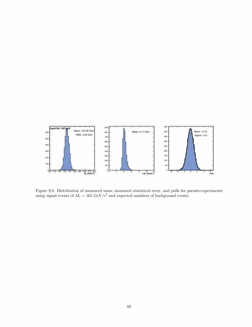
)2 (GeV/ctM130 140 150 160 170 180 190 200 210 2200
100
200
300
400
500
600 Mean: 164.56 GeVRMS: 4.29 GeV
= 165 GeVtInput M
)2 (GeV/ct M!0 2 4 6 8 10 120
100
200
300
400
500
600
700
800
900
Mean: 4.17 GeV
Pull-6 -4 -2 0 2 4 60
50
100
150
200
250
300
350
400
450
Mean: -0.15Sigma: 1.01
Figure 9.8: Distribution of measured mass, measured statistical error, and pulls for pseudo-experimentsusing signal events of Mt = 165 GeV/c2 and expected numbers of background events.
80

CHAPTER 10
Systematic Uncertainties
Our measurement is calibrated using Monte Carlo simulated events. The majority
of systematic uncertainties therefore come from our uncertainty in the accuracy of the
simulation in modeling the data. In this chapter, we describe the facets of the simulation
which may not accurately describe the observed data, and estimate the sensitivity of our
measurement to these effects.
To measure the size of the impact of these uncertainties, our strategy is to perform
pseudo-experiments using a pool of events in which some feature of the events has been
modified. By extracting the average measured mass, we can determine the typical shift
due to these shifted features. In some cases, the magnitude of the shift is smaller than
its statistical error; for these effects we take as a systematic uncertainty, the magnitude
of the statistical error.
10.1 Jet Energy Scale
The measured energy of jets is calibrated using simulated and data events as described
in Chapter 4. Due to lack of knowledge of the underlying processes in hadronization and
limited data statistics, there is an uncertainty in the correction of the raw jet energy.
We vary the response of the jets in simulated events by one unit of the uncertainty in
81

the response, and measure the difference in our extracted top mass.
Sample Measured Mt for M truet = 178.0 GeV/c2
JES +1σ 181.87± 0.73 GeV/c2
JES −1σ 174.86± 0.71 GeV/c2
We take half of the difference between the two measurements, ∆JES = 3.51 GeV/c2. This
is the single largest source of systematic uncertainty in this analysis.
The jet energy scale and its systematic errors are derived primarily for events with
light quark and gluon jets. Studies [52] have demonstrated that in lepton+jets events,
the b-jet energy scale may have up to a 0.6% additional uncertainty. For comparison, we
have measured that moving the b-jet energy scale up by 1% changes the extracted mass
by 1.02 GeV/c2. Thus, we assign an additional uncertainty of 0.61 GeV/c2.
10.2 Generator
We measure the difference in our extracted mass when using events generated with
Pythia and with Herwig.
Sample Measured Mt for M truet = 178.0 GeV/c2
Herwig 177.84± 0.49 GeV/c2
Pythia 178.72± 0.47 GeV/c2
We take the difference between the two measurements, ∆Gen = 0.88± 0.68 GeV/c2.
10.3 Response calibration
The final result depends on the correction derived from our response curve. Uncertainty
in this response translates directly into uncertainty in our result. We vary the response
by 1σ within the statistical uncertainties of the fit, and measure the difference in our
extracted mass.
82
Variation of [offset,slope] (GeV/c2)
Sample [+σ, +σ] [−σ,−σ] [+σ,−σ] [−σ, +σ]
Mt = 170 170.57 170.71 170.95 170.32
Mt = 178 177.67 178.05 178.05 177.66
Mt = 185 184.54 184.15 184.92 184.76
In order to be conservative, we take half of the difference between the pair with the largest
variation, ∆Resp = 0.63 GeV/c2.
10.4 Sample composition
We require a knowledge of the expected signal and background composition of the
sample in order to construct pseudo-experiments from which we extract our response
curve. Given our response curve, we vary the background composition within the quoted
uncertainties and measure the difference in the mean extracted mass of an ensemble
of pseudo-experiments. Note that the uncertainty in the number of expected tt events
includes, and is dominated by, the theoretical uncertainty of 10%.
Varied Sample +σ (GeV/c2) −σ (GeV/c2) ∆Mt/2 (GeV/c2)
tt 177.43 176.08 0.68
Fakes 177.79 177.86 0.04
Z 178.62 177.86 0.38
WW 177.63 177.86 0.12
WZ 177.96 177.86 0.11
Z → ττ 177.90 177.54 0.38
We take these results to indicate that we are not strongly sensitive to the background
composition and thus assign the uncertainty associated with tt as a systematic uncertainty
of ∆Sample = 0.68 GeV/c2.
83

PDF Eigenset0 2 4 6 8 10 12 14 16 18
/2 (G
eV)
+!--
!
-0.1
-0.05
0
0.05
0.1
Figure 10.1: Difference in extracted mass between the positive and negative PDF eigenvectors for aPythia sample.
10.5 PDF uncertainties and αs
To estimate the uncertainty due to the uncertainties in the PDFs, we reweight the
Pythia sample according to 20 sets of positive and negative eigenvectors. We modify
our prescription for forming pseudo-experiments to allow for event weights, in which
events with higher weight are more likely to be chosen for a given pseudo-experiment.
Figure 10.1 shows the 12
difference between the positive and negative eigenvectors. The
total uncertainty added in quadrature is ∆PDF = 0.27 GeV/c2.
In addition, we compare samples with different PDFs, CTEQ5L [43] and MRST72 and
confirm that their central values agree well.
Sample Mt (GeV/c2)
Pythia, CTEQ5L 178.72± 0.47
Pythia, MRST72 178.21± 0.49
Pythia, MRST75 178.05± 0.52
84

The two samples MRST72 and MRST75 [53] use different values of αs to calculate the
PDFs; the difference in these two provides a measure of our sensitivity to the uncertainty in
αs. We estimate our systematic uncertainties due to variation of αs to be ∆αs = 0.15±0.72
GeV/c2.
10.6 Radiation
Our model does not contain any description of initial (ISR) or final state radiation
(FSR), which may contribute significantly to the fraction of mismeasured events. The
rate of initial state radiation can be well studied in Z+jet events, as there is no final state
radiation; the radiation is found to depend smoothly on the energy transfer [52], and can
be examined over a broad range of energies, extending up to the range of tt production. To
measure the uncertainty due to imperfect knowledge of the rate of radiation, we examine
the measured top mass in samples where the simulation parameters are varied by very
conservative amounts. Final state radiation can be probed in the same manner, as it is
described by the same showering algorithm.
Sample Mt (GeV/c2)
Pythia 178.72± 0.47
Pythia, ISR less 177.92± 0.48
Pythia, ISR more 178.53± 0.48
Pythia, FSR less 178.16± 0.49
Pythia, FSR more 178.80± 0.50
We therefore estimate the systematic uncertainty due to modeling of radiation to be
∆ISR = 0.30± 0.34 GeV/c2, and ∆FSR = 0.32± 0.34 GeV/c2.
85
10.7 Background statistics
To measure our dependence on the relatively small background samples, we split each
background sample into twenty pairs of disjoint sets. We measure the mass in the Mt =
178 GeV/c2 sample for each of the disjoint sets and take the root mean square of the
difference between them as an estimate of the uncertainty due to having samples of finite
size. The variation in measured mass for each of the background samples is shown in
Figure 10.2. This is an estimate of the uncertainty due to having samples twice as small
as the samples we use, and so we divide the uncertainty by√
2.
Background RMS(∆Mt)/√
2 (GeV/c2)
Z 0.44
Fakes 0.48
WW 0.13
WZ 0.09
Z → ττ 0.21
We take the sum in quadrature, ∆BGstat = 0.70 GeV/c2.
10.8 Background Modeling
The modeling of the two largest backgrounds may be imperfect; we estimate our sen-
sitivity to possible imperfections in these background models.
10.8.1 Drell-Yan
Drell-Yan production is difficult to model well, as it has a large cross-section and a
small acceptance. Since there is no real missing energy due to escaping neutrinos, there
is a small probability to pass the missing energy requirement. One might be concerned
whether the modeling of large missing energy on the tails of these distributions is accurate.
86

Difference in mass (GeV)-5 -4 -3 -2 -1 0 1 2 3 4 5
Pair
of P
seud
o-Ex
perim
ents
0
2
4
6
8
10
ZZ
Difference in mass (GeV)-5 -4 -3 -2 -1 0 1 2 3 4 5
Pair
of P
seud
o-Ex
perim
ents
0
1
2
3
4
5
6
7 FakesFakes
Difference in mass (GeV)-5 -4 -3 -2 -1 0 1 2 3 4 5
Pair
of P
seud
o-Ex
perim
ents
0
5
10
15
20
25 WWWW
Difference in mass (GeV)-5 -4 -3 -2 -1 0 1 2 3 4 5
Pair
of P
seud
o-Ex
perim
ents
0
5
10
15
20
25
30WZWZ
Difference in mass (GeV)-5 -4 -3 -2 -1 0 1 2 3 4 5
Pair
of P
seud
o-Ex
perim
ents
0
2
4
6
8
10
12
14 !!Z !!Z
Figure 10.2: Variation in measured mass when background samples are split into disjoint sets. Top left,Z; Top right, Fakes. Middle left, WW ; Middle right, WZ. Bottom, Z → ττ .
To gauge our sensitivity to events on the tails of the distribution, we vary the compo-
sition of our pseudo-experiments by both enhancing events and suppressing on events on
the tails. We assign a weight to each event as
w+ = 1 +1√
n+
w0 = 1
87

w− = 1− 1√
n+
where n+ represents the number of events further out on the tail of the missing energy
distribution than the given event. The event with the largest missing energy will receive
weights (w+ = 2, w0 = 1, w− = 0). This enhances or suppresses the tail events.
Weights Mt (GeV/c2)
w+ 177.73± 0.50
w0 177.79± 0.49
w− 177.57± 0.50
As demonstrated by the calibration of the response, the mass measurement suppresses
a good portion of contribution of Zjj events to the extracted mass; this makes the result
less sensitive to variations in the background shape.
We take as the uncertainty due to the shape of this background ∆Drell−Y anShape = 0.22
GeV/c2.
10.8.2 Fake background
The fake background is very difficult to model well in the simulation, as it is sensitive
to the smallest details of the detector performance. To avoid issues of modeling, the
events which imitate this background are drawn from the data itself; the events are
selected with a looser requirement on one of the leptons in order to accumulate a sample
of fake candidates, and then weighted by the probability that the loose lepton would
pass lepton identification requirements. These weights are calculated as a function of the
PT and isolation of the fake candidate, and each candidate has its own weight (w) and
uncertainty (∆w).
To gauge our sensitivity to the calculation of the fake rates, we vary the fake rates in
two ways. First (a), we enhance those events with large fake probability, to exaggerate
88

their effect; second (b), we enhance events with small fake probability, to exaggerate their
effect:
Mode w > w w < w
a w → w + ∆w w → w −∆w
b w → w −∆w w → w + ∆w
We study the effect of this weighting on fully realistic pseudo-experiments:
Weights Mt (GeV/c2)
wa 177.83± 0.49
default 177.84± 0.49
wb 177.76± 0.49
As argued above, the mass measurement is reasonably successful at reducing the effect
of these background events, which makes the extracted mass less sensitive to their shapes.
We take the difference as our systematic uncertainty, ∆fakesShape = 0.08 GeV/c2, and the
total shape uncertainty to be the two in quadrature
∆Shape = 0.23 GeV/c2.
10.9 Lepton Energy Scale
Studies have shown that the Monte Carlo has an energy scale for electrons that is up
to 0.5% higher than that in data. As the Monte Carlo events we use do not include a
scale factor to account for this effect, we measure an associated systematic uncertainty
by varying the lepton energy scale in Monte Carlo events by ±1%.
Sample Measured Mt for M truet = 178.0 GeV/c2
LES +1% 177.54± 0.49 GeV/c2
LES −1% 177.29± 0.48 GeV/c2
89

Source SizeJet Energy Scale 3.5 GeV/c2
B-jet energy scale 0.6 GeV/c2
Generator 0.9 GeV/c2
Response uncertainty 0.6 GeV/c2
Sample composition uncertainty 0.7 GeV/c2
Background statistics 0.7 GeV/c2
Background modeling 0.2 GeV/c2
ISR modeling 0.3 GeV/c2
FSR modeling 0.3 GeV/c2
PDFs 0.3 GeV/c2
αs 0.2± 0.7 GeV/c2
Lepton Energy Scale 0.1 GeV/c2
Total 3.9 GeV/c2
Table 10.1: Summary of systematic uncertainties
We take half of the difference between the two measurements, ∆LES = 0.13 GeV/c2.
10.10 Summary
The systematic uncertainties measured in the previous sections are summarized in
Table 10.1. Our total systematic uncertainty is 3.9 GeV/c2.
90

CHAPTER 11
Measurement in Data
The measurement in data is performed with a sample of∫
Ldt = 1.0 fb−1. This sample
contains 78 candidate events passing the selection cuts outlined in Chapter 4. Their run,
event numbers and a summary of their kinematic properties can be found in Appendix
A, Tables A.1- A.3.
11.1 Kinematic Properties of Observed Events
We examine the events observed in the data and compare their kinematic properties
to those predicted from the simulation; the latter is the sum of signal and background
contributions.
Examining the kinematic distributions in Appendix A (see Figures A.1-A.14) does not
reveal any dramatic deviation in shape for any variable.
In addition, we compare the expected probability distributions of tt, Zjj, Fake and
WWjj probabilities to the observed events, see Figures 11.1-11.4. These quantities are
sensitive to all of the kinematic information in the event, and show no significant shape
discrepancies.
91

=165)]/dx]t[tt(M!ln[d-70 -60 -50 -40 -30 -20 -10 0
Even
ts
0
5
10
15
20
25CDF II Preliminary
(78 events)-1 Ldt = 1.0 fb")2=165 GeV/cttt (M
FakesWWWZ
##$ZZData
Figure 11.1: Comparison of the tt probability distribution for simulated events, scaled by expectedcontribution to the sample composition, to that for observed events.
(Zjj)/dx]!ln[d-90 -80 -70 -60 -50 -40 -30 -20 -10 0
Even
ts
0
5
10
15
20
25
30CDF II Preliminary
(78 events)-1 Ldt = 1.0 fb")2=165 GeV/cttt (M
FakesWWWZ
##$ZZData
Figure 11.2: Comparison of the Zjj probability distribution for simulated events, scaled by expectedcontribution to the sample composition, to that for observed events.
92
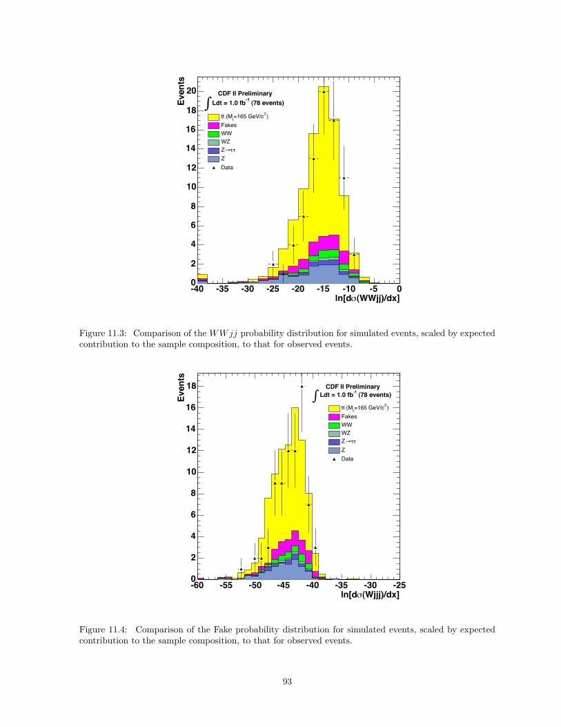
(WWjj)/dx]!ln[d-40 -35 -30 -25 -20 -15 -10 -5 0
Even
ts
0
2
4
6
8
10
12
14
16
18
20 CDF II Preliminary (78 events)-1 Ldt = 1.0 fb"
)2=165 GeV/cttt (MFakesWWWZ
##$ZZData
Figure 11.3: Comparison of the WWjj probability distribution for simulated events, scaled by expectedcontribution to the sample composition, to that for observed events.
(Wjjj)/dx]!ln[d-60 -55 -50 -45 -40 -35 -30 -25
Even
ts
0
2
4
6
8
10
12
14
16
18 CDF II Preliminary (78 events)-1 Ldt = 1.0 fb"
)2=165 GeV/cttt (MFakesWWWZ
##$ZZData
Figure 11.4: Comparison of the Fake probability distribution for simulated events, scaled by expectedcontribution to the sample composition, to that for observed events.
93

11.2 Result
The 78 candidate events in the data have individual posterior probabilities as seen in
Figures 11.5-11.7. From the joint probability, we extract the uncorrected, unscaled mass,
M rawt = 165.11± 2.82raw,unscaled GeV/c2
After applying the response correction and the error scaling as described in Chapter 9,
the final result is
Mt = 164.49± 3.94 GeV/c2
The posterior probability curve can be seen in Figure 11.8. The error we measure is not
unexpected when one considers the central value; in pseudo-experiments where Mt = 165
GeV/c2, 46% of the errors are smaller than this value, see Figure 11.9.
We can validate the measured mass by measuring Mt separately in events with two
electrons, events with two muons and events with both an electron and a muon. These
results are shown in Figure 11.10 and are all consistent with one another.
94

121.1 174.5 227.9
Arbi
trary
Uni
ts
0
1
121.1 174.5 227.90
1
121.1 174.5 227.90
1
121.1 174.5 227.90
1
121.1 174.5 227.90
1
121.1 174.5 227.9
Arbi
trary
Uni
ts
0
1
121.1 174.5 227.90
1
121.1 174.5 227.90
1
121.1 174.5 227.90
1
121.1 174.5 227.90
1
121.1 174.5 227.9
Arbi
trary
Uni
ts
0
1
121.1 174.5 227.90
1
121.1 174.5 227.90
1
121.1 174.5 227.90
1
121.1 174.5 227.90
1
121.1 174.5 227.9
Arbi
trary
Uni
ts
0
1
121.1 174.5 227.90
1
121.1 174.5 227.90
1
121.1 174.5 227.90
1
121.1 174.5 227.90
1
121.1 174.5 227.9
Arbi
trary
Uni
ts
0
1
121.1 174.5 227.90
1
121.1 174.5 227.90
1
121.1 174.5 227.90
1
121.1 174.5 227.90
1
121.1 174.5 227.9
Arbi
trary
Uni
ts
0
1
121.1 174.5 227.90
1
121.1 174.5 227.90
1
121.1 174.5 227.90
1
121.1 174.5 227.90
1
]2Top Pole Mass [GeV/c121.1 174.5 227.9
Arbi
trary
Uni
ts
0
1
]2Top Pole Mass [GeV/c121.1 174.5 227.90
1
]2Top Pole Mass [GeV/c121.1 174.5 227.90
1
Figure 11.5: Posterior probabilities for each of the 33 candidate events found in 340 pb−1 of datacollected between March 2002 and August 2004. Each includes the normalized signal and backgroundprobabilities.
95

121.1 174.5 227.9
Arbi
trary
Uni
ts
0
1
121.1 174.5 227.90
1
121.1 174.5 227.90
1
121.1 174.5 227.90
1
121.1 174.5 227.9
Arbi
trary
Uni
ts
0
1
121.1 174.5 227.90
1
121.1 174.5 227.90
1
121.1 174.5 227.90
1
121.1 174.5 227.9
Arbi
trary
Uni
ts
0
1
121.1 174.5 227.90
1
121.1 174.5 227.90
1
121.1 174.5 227.90
1
121.1 174.5 227.9
Arbi
trary
Uni
ts
0
1
121.1 174.5 227.90
1
121.1 174.5 227.90
1
121.1 174.5 227.90
1
121.1 174.5 227.9
Arbi
trary
Uni
ts
0
1
121.1 174.5 227.90
1
121.1 174.5 227.90
1
121.1 174.5 227.90
1
121.1 174.5 227.9
Arbi
trary
Uni
ts
0
1
121.1 174.5 227.90
1
121.1 174.5 227.90
1
121.1 174.5 227.90
1
121.1 174.5 227.9
Arbi
trary
Uni
ts
0
1
121.1 174.5 227.90
1
121.1 174.5 227.90
1
121.1 174.5 227.90
1
]2Top Pole Mass [GeV/c121.1 174.5 227.9
Arbi
trary
Uni
ts
0
1
]2Top Pole Mass [GeV/c121.1 174.5 227.90
1
]2Top Pole Mass [GeV/c121.1 174.5 227.90
1
Figure 11.6: Posterior probabilities for each of the 31 candidate events found in the 400 pb−1 of data col-lected between December 2004 and September 2005. Each includes the normalized signal and backgroundprobabilities.
96

121.1 174.5 227.9
Arbi
trary
Uni
ts
0
1
121.1 174.5 227.90
1
121.1 174.5 227.90
1
121.1 174.5 227.9
Arbi
trary
Uni
ts
0
1
121.1 174.5 227.90
1
121.1 174.5 227.90
1
121.1 174.5 227.9
Arbi
trary
Uni
ts
0
1
121.1 174.5 227.90
1
121.1 174.5 227.90
1
121.1 174.5 227.9
Arbi
trary
Uni
ts
0
1
121.1 174.5 227.90
1
121.1 174.5 227.90
1
]2Top Pole Mass [GeV/c121.1 174.5 227.9
Arbi
trary
Uni
ts
0
1
]2Top Pole Mass [GeV/c121.1 174.5 227.90
1
Figure 11.7: Posterior probabilities for each of the 14 candidate events found in the 260 pb−1 of data col-lected between September 2005 and February 2006. Each includes the normalized signal and backgroundprobabilities.
97

)2 (GeV/ctM145 150 155 160 165 170 175 180 185
)2 (GeV/ctM145 150 155 160 165 170 175 180 185
Prob
abili
ty D
ensi
ty
0
0.02
0.04
0.06
0.08
0.1
0.12
0.14
0.16CDF II Preliminary
(78 events)-1 Ldt = 1.0 fb!
Figure 11.8: Final posterior probability density as a function of the top pole mass for the 78 candidateevents in the data.
)2 (GeV/ct M!0 2 4 6 8 10 12
Ense
mbl
e Re
sult
0
100
200
300
400
500
600
700
800
900)2=165 GeV/ctHerwig tt (M
This measurement
CDF II Preliminary (78 events)-1 Ldt = 1.0 fb"
Figure 11.9: Distribution of expected errors for Mt = 165 GeV/c2. The measured error is shows as theline; 46% of pseudo-experiments yield a smaller error.
98

)2Top mass (GeV/c140 145 150 155 160 165 170 175 180 1850
All 3.9±164.5 (78 events)
e-e 12.9±162.0 (15 events)
µ-µ 7.0±164.5 (26 events)
µe- 5.3±164.6 (37 events)
(stat. error only))-1CDF II Preliminary (1.0 fb
Figure 11.10: Measurement of the top quark mass in ee, µµ and eµ events separately. The measurementin all data events is also shown for comparison. Only statistical uncertainties are shown.
99

CHAPTER 12
Conclusion
We have measured the mass of the top quark in the dilepton decay channel. Using
1.0 fb−1 of Run II data collected at the CDF detector, we measure:
Mt = 164.5± 3.9(stat.)± 3.9(syst.)GeV/c2.
This result shows little deviation from the previously published result in this chan-
nel [2],
Mt = 165.2± 6.1(stat.)± 3.4(syst.)GeV/c2,
which uses 340 pb−1 of data. It is also consistent with recently published template-based
measurements of the top quark mass in this channel [54],
Mt = 170.1± 6.0(stat.)± 4.1(syst.)GeV/c2,
which uses up to 360 pb−1 of data. Our measured value is smaller than recent template-
based measurements in the lepton+jets channel [55],
Mt = 173.4± 2.5(stat.+JES)± 1.3(syst.)GeV/c2,
using 680 pb−1. This deviation is not inconsistent with a statistical fluctuation [18]. The
possibility of this deviation being a fluctuation is further enforced by the most recent
100

preliminary measurement of the top quark mass in the lepton+jets channel [56],
Mt = 170.9± 2.2(stat.+JES)± 1.4(syst.)GeV/c2,
which uses 940 pb−1 of data and a matrix-element method. More data will be needed to
tell whether a significant deviation exists amongst channels.
Additionally, we can apply secondary vertex tagging to identify b-quarks in the dilepton
sample used in this analysis. The requirement of a b-tag results in a subset of the dilepton
sample with a signal-to-background ratio of 20:1 despite the loss of 40% of the expected
signal statistics. The resulting sample can be used to verify our measurement of the
top quark mass in the dilepton channel in a near background-free sample. Applying the
same mass measurement technique to this b-tagged sample (we use the secvtx tagging
algorithm, described in Ref. [57]), we measure [58]:
Mt = 167.3± 4.6(stat)± 3.8(syst.)GeV/c2.
This result is consistent with the measurement made in the full sample.
The measurement described in this dissertation is included as part of a combination
performed using measurements from both CDF and DØ in all decay channels [59]:
Mt = 171.4± 1.2(stat.)± 1.8(syst.)GeV/c2.
In this combination, our measurement contributes a weight of 4.8%. Using this evaluation
of the top quark mass and other precision electroweak measurements the constraints on
the standard model Higgs Boson are [60]:
MH = 85+39−28 GeV/c2
MH < 166 GeV/c2 at 95% CL.
101

We anticipate that the method used to make this measurement will result in a statistical
uncertainty of 2 GeV/c2 with 4 fb−1 of data. Systematic uncertainties will be dominant
at this level. Several improvements to the method are in progress, including:
• Using a selection criteria based on genetically evolving neural networks, optimized
for measurements of the top quark mass.
• Using events from the decay Z → bb to calibrate the b-jet energy scale, allowing for
a reduction in the jet energy scale systematic uncertainty.
In addition, accumulating more data will help reduce the uncertainty associated with
background estimates that rely on data events, such as fakes and Z/γ∗ → ee, µµ. Assum-
ing 8 fb−1 of data can be accumulated by the end of Run II, an overall uncertainty of less
than 1.5 GeV/c2 for a combined measurement of the top quark mass is possible.
102
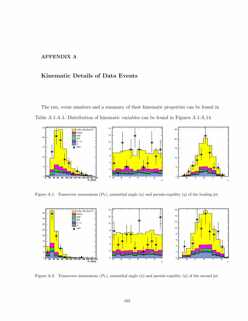
APPENDIX A
Kinematic Details of Data Events
The run, event numbers and a summary of their kinematic properties can be found in
Table A.1-A.3. Distribution of kinematic variables can be found in Figures A.1-A.14.
[GeV]TP0 20 40 60 80 100 120 140 160 180 200 220 2400
5
10
15
20
25)2=165 GeV/cttt (M
FakesWWWZ
!!"ZZdata
#-3 -2 -1 0 1 20
2
4
6
8
10
12
14
$-3 -2 -1 0 1 20
5
10
15
20
25
Figure A.1: Transverse momentum (PT ), azimuthal angle (φ) and pseudo-rapidity (η) of the leading jet.
[GeV]TP0 20 40 60 80 100 120 140 160 180 200 220 2400
5
10
15
20
25
30
35
40)2=165 GeV/cttt (M
FakesWWWZ
!!"ZZdata
#-3 -2 -1 0 1 20
2
4
6
8
10
12
14
$-3 -2 -1 0 1 20
2
4
6
8
10
12
14
16
Figure A.2: Transverse momentum (PT ), azimuthal angle (φ) and pseudo-rapidity (η) of the second jet.
103

PT [GeV/c] ET [GeV] 6ET
Run Event Lepton 1 Lepton 2 Jet 1 Jet 2 [GeV] Njets
177491 3807306 25.94 21.03 67.44 42.8 79.22 3178738 1660363 99.99 60.59 42.67 36.52 90.26 3143257 760520 27.29 20.96 43.87 36.79 92.24 4150431 368759 58.27 36.19 54.85 32.56 44.07 4150435 2896171 45.37 42.88 88.21 44.22 64.71 2155114 478702 34.48 28.47 73.59 36.02 89.96 3156484 3099305 35.17 34.31 66.91 34.22 75.91 3150418 960369 91.38 89.48 30.67 25.99 68.66 2151978 507773 35.89 34.72 47.04 45.7 91.35 2153374 2276742 72.02 56.87 85.76 55.15 58.14 3161633 963604 40.24 26.49 62.27 36.36 60.52 3165364 592961 47.35 21.59 78.9 47.31 127.9 3166063 2833132 41.36 38.04 49.73 49.62 64.97 2167053 12011678 75.77 50.43 86.61 26.31 28.47 3167631 2058969 33.97 31.34 38.33 36.65 61.32 2167629 180103 96.57 78.59 77.06 35.49 28.4 2168599 2964061 40.76 23.68 35.7 33.45 96.85 3183963 1259645 84.72 27.04 142.1 28.9 63.14 2184779 892809 51.1 46.9 46.05 20.01 48.86 2184289 101220 147.8 49.19 135.1 38.71 29.67 2186598 1618142 69.41 35.75 70.19 68.91 66.96 3186598 4194951 54.5 36.05 90.35 58.62 42.65 2178540 2208375 64.42 34.77 96.19 42.62 53.59 2178738 10340757 50.05 21.39 75.71 36.06 88.4 2153325 599511 37.11 25.23 50.78 34.32 46.47 3153447 2643751 87.45 26.3 106.4 20.98 35.52 3154654 7344016 59.42 52.86 36.43 19.96 56.66 3160988 385505 26.05 21.02 87.15 56.91 32.19 2162820 7050764 33.46 26.24 65.95 52.41 95.84 2163012 1438203 119.1 98.54 103.8 73.67 80.55 2165198 1827962 34.48 23.82 63.08 31.83 101.4 2185037 2287335 85.73 56.09 65.78 60.03 26.92 2185377 103906 76 20.87 69.53 26.34 80.59 2
Table A.1: Run and event numbers and some kinematic quantities for the 33 candidate events found in340 pb−1 of data collected between March 2002 and August 2004.
104

PT [GeV/c] ET [GeV] 6ET
Run Event Lepton 1 Lepton 2 Jet 1 Jet 2 [GeV] Njets
193031 7271850 94.82 42.06 76.9 64.41 103 2193032 1657759 69.74 43.75 40.1 16.31 70.32 2193051 1108405 114.1 60.28 40.05 39.72 55.01 2193892 345334 75.91 50.23 142.3 31.74 116.5 3194590 4487208 65.96 34.23 51.62 44.88 90.77 3196902 291907 25.06 23.86 56.24 27.19 69.67 3196170 1783955 44.93 33.17 109.9 39.17 55.08 2196473 3624629 36.67 26.96 53.77 34.69 51.88 3196902 1636420 34.79 24.94 166.5 64.69 50.15 4195742 628424 67.02 23.05 54.43 49.66 67.58 4198082 4507326 30.64 22.66 105.2 64.17 25.77 3197404 240811 87.96 51.25 33.14 18.31 78.74 3198695 5284824 109 81.18 74.63 41.11 40.93 2198710 4284073 39.7 25.56 52.52 44.92 57.89 4202135 5684094 34.61 32.99 26.7 23.7 57.16 4202514 4625226 52.84 34.79 37.7 36.95 79.06 2203265 2621856 32.84 21.37 96.81 55.72 87.55 3193901 1732074 146.9 76.4 32.5 32.07 31.12 2193901 1851653 76.88 27.09 117.9 15.83 91.4 2191545 898092 58.75 33.64 79.17 64.26 45.53 5192348 8119187 120.4 37.35 156.5 21.3 109.9 2193991 1042119 45.31 34.51 74.95 60.55 80.07 2195341 4235173 43.63 26.5 46.68 40.44 109.2 2198340 192801 47.55 28.39 90.26 52.81 56.23 2197808 6530989 57.85 33.78 39.85 20.67 63.05 2196663 714179 61.08 36.59 30.35 24.74 56.98 3202771 5737518 48.85 24.36 72.86 26.07 62.12 3202397 204913 53.87 33.56 58.92 37.08 25.55 3203764 2353176 39.65 31.2 165 96.52 93.98 3199650 2833299 79.63 38.44 127.1 61.65 52.95 2199655 1714860 35.16 22.61 64.12 50.29 71.22 2
Table A.2: Run and event numbers and some kinematic quantities for events found in the 400 pb−1 ofdata collected between December 2004 and September 2005.
105

PT [GeV/c] ET [GeV] 6ET
Run Event Lepton 1 Lepton 2 Jet 1 Jet 2 [GeV] Njets
206723 7731509 31.28 25.01 100.8 17.38 74.9 2206836 1380873 38.9 23.63 58.04 40.29 71.4 3204111 59242 56.46 49.33 39.74 21.91 33.64 2205009 1907663 41.66 25.84 25.29 22.2 25.73 6204640 4116811 56.62 41.22 102 31.76 63.77 2205324 1393300 65.22 25.47 88.32 42.01 127.4 2209191 2272489 121.4 81.12 24.8 17.12 44.36 2210008 7652752 50.66 46.37 55.64 34.38 64.92 3207156 2387787 41.77 26.14 47.88 31.3 95.6 2209263 3986598 32.78 25.1 188.3 177.8 47.96 4203819 7922132 63.86 36.84 69.81 36.56 41.47 2205628 2185064 162 97.41 52.12 35.29 66.84 3203824 196206 139.1 20.85 58.01 22.96 58.05 2207079 11915785 37.84 33.52 99.8 30.88 108.1 3
Table A.3: Run and event numbers and some kinematic quantities for cthe 14 candidate events found inthe 260 pb−1 of data collected between September 2005 and February 2006.
[GeV]TP0 20 40 60 80 1000
2
4
6
8
10
12
14 )2=165 GeV/cttt (MFakesWWWZ
!!"ZZdata
#-3 -2 -1 0 1 20
1
2
3
4
5
6
7
8
9
$-3 -2 -1 0 1 20
1
2
3
4
5
6
7
8
Figure A.3: Transverse momentum (PT ), azimuthal angle (φ) and pseudo-rapidity (η) of the third jet.
[GeV]TP0 20 40 60 80 100 120 140 160 180 200 220 240
0
5
10
15
20
25
30
)2
=165 GeV/ct
tt (M
Fakes
WW
WZ
!!"Z
Z
data
#-3 -2 -1 0 1 2
0
2
4
6
8
10
12
$-3 -2 -1 0 1 2
0
5
10
15
20
25
Figure A.4: Transverse momentum (PT ), azimuthal angle (φ) and pseudo-rapidity (η) of the leadinglepton.
106

[GeV]TP0 20 40 60 80 100 120 140 160 180 200 220 2400
10
20
30
40
50
60)2=165 GeV/cttt (M
FakesWWWZ
!!"ZZdata
#-3 -2 -1 0 1 20
2
4
6
8
10
12
$-3 -2 -1 0 1 20
2
4
6
8
10
12
14
16
18
20
22
Figure A.5: Transverse momentum (PT ), azimuthal angle (φ) and pseudo-rapidity (η) of the secondlepton.
[GeV]TP0 50 100 150 200 250 300 350 400 4500
5
10
15
20
25
30
35
40
45 )2=165 GeV/cttt (MFakesWWWZ
!!"ZZdata
#-3 -2 -1 0 1 20
2
4
6
8
10
$-3 -2 -1 0 1 20
10
20
30
40
50
60
70
80
90
Figure A.6: Transverse momentum (PT ), azimuthal angle (φ) and pseudo-rapidity (η) of the missingtransverse energy.
[GeV]TP0 20 40 60 80 100 120 140 160 180 200 220 2400
5
10
15
20
25)2=165 GeV/cttt (M
FakesWWWZ
!!"ZZdata
#-3 -2 -1 0 1 20
2
4
6
8
10
12
$-3 -2 -1 0 1 20
2
4
6
8
10
12
14
16
18
20
22
Figure A.7: Transverse momentum (PT ), azimuthal angle (φ) and pseudo-rapidity (η) of the vector sumof the leptons.
107

[GeV]TP0 20 40 60 80 100 120 140 160 180 200 220 2400
5
10
15
20
25
30
35
40)2=165 GeV/cttt (M
FakesWWWZ
!!"ZZdata
#-3 -2 -1 0 1 20
2
4
6
8
10
12
14
$-3 -2 -1 0 1 20
5
10
15
20
25
Figure A.8: Difference in transverse momentum (PT ), azimuthal angle (φ) and pseudo-rapidity (η) ofthe two leptons.
[GeV]TP0 20 40 60 80 100 120 140 160 180 200 220 2400
2
4
6
8
10
12
14
16
18)2=165 GeV/cttt (M
FakesWWWZ
!!"ZZdata
#-3 -2 -1 0 1 20
2
4
6
8
10
12
$-3 -2 -1 0 1 20
2
4
6
8
10
12
14
Figure A.9: Transverse momentum (PT ), azimuthal angle (φ) and pseudo-rapidity (η) of the vector sumof the jets.
108

[GeV]tH0 100 200 300 400 500 600 700 800 900 10000
5
10
15
20
25
30
35)2=165 GeV/cttt (M
FakesWWWZ
!!"ZZdata
N. of Jets0 1 2 3 4 5 6 7 8 90
10
20
30
40
50
60)2=165 GeV/cttt (M
FakesWWWZ
!!"ZZdata
Figure A.10: Distribution of HT and Njets.
109

Transverse Unclustered Energy [GeV]0 20 40 60 80 100 120 140 160
Even
ts
0
5
10
15
20
25
30
)2=165 GeV/cttt (MFakesWWWZ
!!"ZZdata
CDF II Preliminary (78 events)-1 Ldt = 1.0 fb#
Figure A.11: Distribution of transverse unclustered energy.
[GeV]TP0 20 40 60 80 100 120 140 160 180 200 220 2400
5
10
15
20
25
30
35 )2=165 GeV/cttt (MFakesWWWZ
!!"ZZdata
#-3 -2 -1 0 1 20
2
4
6
8
10
$-3 -2 -1 0 1 20
2
4
6
8
10
12
14
Figure A.12: Transverse momentum (PT ), azimuthal angle (φ) and pseudo-rapidity (η) of the differencebetween the leading jets.
110

[GeV]TP0 20 40 60 80 100 120 140 160 180 200 220 2400
5
10
15
20
25
30
)2=165 GeV/cttt (MFakesWWWZ
!!"ZZdata
#-3 -2 -1 0 1 20
2
4
6
8
10
12
14
$-3 -2 -1 0 1 20
10
20
30
40
50
60
70
80
90
Figure A.13: Transverse momentum (PT ), azimuthal angle (φ) and pseudo-rapidity (η) of the differencebetween the missing energy and the leading jet.
[GeV]TP0 20 40 60 80 100 120 140 160 180 200 220 2400
5
10
15
20
25
30)2=165 GeV/cttt (M
FakesWWWZ
!!"ZZdata
#-3 -2 -1 0 1 20
2
4
6
8
10
$-3 -2 -1 0 1 20
2
4
6
8
10
12
14
16
18
20
Figure A.14: Transverse momentum (PT ), azimuthal angle (φ) and pseudo-rapidity (η) of the vectorsum of both jets and leptons.
111

BIBLIOGRAPHY
[1] A. Kovalev, Measurement of the top quark mass at CDF II, PhD thesis, University of Pennsylvania,2005. 2
[2] A. Abulencia et al., Top quark mass measurement from dilepton events at CDF II, Phys. Rev.Lett., 96 (2006). 2, 100
[3] D. J. Gross and F. Wilczek, Asymptotically free gauge theories, Phys. Rev., D8 (1973), p. 3633.3
[4] H. D. Politzer, Asymptotic freedom: An approach to strong interactions, Phys. Rept., 14 (1974),p. 129. 3
[5] S. L. Glashow, Partial symmetries of weak interactions, Nucl. Phys., 22 (1961). 3
[6] A. Salam and J. C. Ward, Electromagnetic and weak interactions, Phys. Lett., 13 (1964). 3
[7] S. Weinberg, A model of leptons, Phys. Rev. Lett., 19 (1967), p. 1264. 3
[8] S. Eidelman et al., Review of particle physics, Physics Letters B, 592 (2004), p. 1. 4, 33
[9] P. W. Higgs, Broken symmetries and the masses of gauge bosons, Phys. Rev. Lett., 13 (1964),p. 508. 4
[10] R. Barate et al., Search for the standard model Higgs boson at LEP, Phys. Lett., B565 (2003),p. 61. 5
[11] The LEP Collaboration, The LEP Electroweak Working group, The SLD Elec-troweak and Heavy Flavor Groups, A combination of preliminary electroweak measurementsand constraints on the standard model, Tech. Report CERN-PH-EP/2005-051, CERN, 2005. viii,5, 6
[12] E. Rice et al., Search for structure in σ(e+e− → hadrons) between√
s =10.34 and 11.6 GeV,Phys. Rev. Lett., 48 (1982), p. 906. 6
[13] F. Abe et al., Observation of top quark production in pp collisions with the Collider Detector atFermilab, Phys. Rev. Lett., 74 (1995), p. 2626. 6
[14] S. Abachi et al., Observation of the top quark, Phys. Rev. Lett., 74 (1995), p. 2632. 6
[15] M. Cacciari et al., The tt cross-section at 1.8 and 1.96 TeV: A study of the systematics due toparton densities and scale dependence, J. High Energy Phys., 0404 (2004), p. 068. viii, xiii, 7, 8, 35,37, 53, 74
[16] CDF Collaboration, Combination of CDF top quark pair production cross section measurementsup to 750 pb−1, Tech. Report CDF/PHYS/TOP/PUBLIC/8148, CDF Collaboration, 2006. viii, 7,8
112

[17] M. Kobayashi and T. Maskawa, CP violation in the renormalizable theory of weak interaction,Prog. Theor. Phys., 49 (1973), p. 652. 7
[18] The CDF Collaboration, The DØ Collaboration and Tevatron Electroweak Work-ing Group, Combination of CDF and DØ results on the mass of the top quark, Tech. ReportFERMILAB-RM-2347-E, Fermilab, 2006. viii, 11, 12, 100
[19] F. Abe et al., The CDF II detector: Technical design report, Tech. Report FERMILAB-Pub-96/390-E, 1996. viii, 19, 22
[20] A. Sill et al., SVX-II: CDF Run II silicon tracking projects, Nucl. Instrum. Methods, A447 (2000),p. 1. 20
[21] C. S. Hill et al., L00: Operational experience and performance of the CDF II silicon detector,Nucl. Instrum. Methods, A530 (2004), p. 1. 21
[22] A. Affolder et al., ISL: Intermediate silicon layers detector for the CDF experiment, Nucl.Instrum. Methods, A453 (2000), p. 84. 21
[23] T. Affolder et al., COT central outer tracker, Nucl. Instrum. Methods, A526 (2004), p. 249. 22
[24] L. Balka et al., The CDF central electromagnetic calorimeter, Nucl. Instrum. Methods, A267(1988), p. 272. 24
[25] S. Bertolucci et al., The CDF central and endwall hadronic calorimeters, Nucl. Instrum. Meth-ods, A267 (1988), p. 301. 24
[26] M. Albrow et al., The CDF plug upgrade electromagnetic calorimeter: Test beam result, Nucl.Instrum. Methods, A480 (2002), p. 524. 24
[27] G. Apollinari et al., Shower maximum detector for the CDF plug upgrade calorimeter, Nucl.Instrum. Methods, A412 (1998), p. 515. 24
[28] G. Ascoli et al., The CDF central muon detector, Nucl. Instrum. Methods, A268 (1988), p. 33.25
[29] D. Acosta et al., Measurement of the tt production cross section in pp collisions at√
s = 1.96TeV using dilepton events, Phys. Rev. Lett., 93 (2004), p. 142001. 29
[30] , Measurement of the forward-backward charge asymmetry from W → eν production in ppcollisions at
√s=1.96 TeV, Phys. Rev. D, 71 (2005), p. 051104. 30
[31] F. Abe et al., Topology of three-jet events in pp collisions at√
s = 1.8 TeV, Phys. Rev. D, 45(1992), p. 1448. 31
[32] A. Bhatti et al., Determination of the jet energy scale at the Collider Detector at Fermilab, Nucl.Instrum. Methods, A (To be published). 32
[33] T. Sjostrand et al., High-energy-physics event generation with PYTHIA 6.1, Computer Phys.Commun., 135 (2001), p. 238. ix, 32
[34] G. Corcella et al., HERWIG 6: an event generator for hadron emission reactions with interferinggluons, J. High Energy Phys., 01 (2001), p. 010. ix, 32, 36, 37
[35] M. L. Mangano et al., ALPGEN, a generator for hard multiparton processes in hadronic colli-sions, J. High Energy Phys., 0307 (2003), p. 001. 35
[36] F. Abe et al., Measurement of the top quark mass with the Collider Detector at Fermilab, Phys.Rev. Lett., 82 (1999), p. 271. 38
113
[37] B. Abbot et al., Measurement of the top quark mass using dilepton events, Phys. Rev. Lett., 80(1998), p. 2063. 38
[38] K. Kondo, Dynamical likelihood method for reconstruction of events with missing momentum. I.Method and toy models, J. Phys. Soc. Jpn., 57 (1988), p. 4126. 38
[39] G. Goldstein et al., Observing top-quark production at the Fermilab Tevatron, Phys. Rev. D, 47(1993), p. 967. 38
[40] V. Abazov et al., A precision measurement of the mass of the top quark, Nature, 429 (2004),p. 638. 39
[41] F. Canelli, Helicity of W bosons in single lepton tt events, PhD thesis, University of Rochester,2003. 39, 44
[42] J. Estrada, Maximal Use of Kinematic Information for the Extraction of the Mass of the TopQuark in Single-Lepton tt events at DØ, PhD thesis, University of Rochester, 2001. 39
[43] J. Pumplin et al., New generation of parton distributions with uncertainties from global QCDanalysis, J. High Energy Phys., 007 (2002), p. 012. 40, 84
[44] G. Mahlon and S. Parke, Maximizing spin correlations in top quark pair production at theTevatron, Phys. Lett. B, 411 (1997), p. 173. 52
[45] , Improved spin basis for angular correlation studies in single top quark production at theFermilab Tevatron, Phys. Rev. D, 55 (1997), p. 7249. 52
[46] K. G. Chetyrkin et al., Second order QCD corrections to Γ(t → Wb), Phys. Rev. D, 60 (1999).53
[47] C. Sturm, Memoire sur la resolution des equations numeriques, Bull. Sci. Math. Ferussac, 2 (1829),p. 419. 55
[48] G. P. Lepage, A new algorithm for adaptive multidimensional integration, Journal of Computa-tional Physics, 27 (1978), p. 192. 58
[49] M. Galassi et al., GNU Scientific Library Reference Manual (2nd Ed.), Network Theory Ltd.,2004. 58
[50] A. Pukhov et al., CompHEP – a package for evaluation of Feynman diagrams and integrationover multi-particle phase space, Tech. Report INP MSU 98-41/542, Moscow State University, 1999.64
[51] F. Maltoni and T. Stelzer, Madevent: Automatic event generation with MadGraph, J. HighEnergy Phys., 0302 (2003). 64
[52] A. Abulencia et al., Top quark mass measurement using the template method in the lepton+jetschannel at CDF, Phys. Rev. D, 73 (2006), p. 32003. 82, 85
[53] A. D. Martin et al., The αs dependence of parton distributions, Phys. Lett. B, 356 (1995), p. 89.85
[54] A. Abulencia et al., Measurement of the top quark mass using template methods on dileptonevents in pp collisions at
√s=1.96 TeV, Phys. Rev. D, 73 (2006), p. 112006. 100
[55] CDF Collaboration, Measurement of the top quark mass using the template method inthe lepton plus jets channel with in situ W → jj calibration at CDF II, Tech. ReportCDF/PHYS/TOP/PUBLIC/8125, CDF Collaboration, 2006. 100
114

[56] , Measurement of the top quark mass using the matrix element analysis technique in the leptonplus jets channel with in situ W → jj calibration, Tech. Report CDF/PHYS/TOP/PUBLIC/8375,CDF Collaboration, 2006. 101
[57] D. Acosta et al., Measurement of the tt production cross section in p[overline p] collisions at√s = 1.96 TeV using lepton + jets events with secondary vertex b -tagging, Phys. Rev. D, 71 (2005),
p. 052003. 101
[58] CDF Collaboration, Measurement of the top quark mass using a matrix element method in ab-tagged sample, Tech. Report CDF/PHYS/TOP/PUBLIC/8401, CDF Collaboration, 2006. 101
[59] The CDF Collaboration, The DØ Collaboration and Tevatron Electroweak Work-ing Group, Combination of CDF and DØ results on the mass of the top quark, Tech. ReportFERMILAB-RM-2355-E, Fermilab, 2006. 101
[60] LEP Electroweak Working Group, http://lepewwg.web.cern.ch/LEPEWWG/, 2006. 101
115